the Creative Commons Attribution 4.0 License.
the Creative Commons Attribution 4.0 License.
 | 07 Jul 2021
Aeroelastic loads on a 10 MW turbine exposed to extreme events selected from a year-long large-eddy simulation over the North Sea
Gerard Schepers
Pim van Dorp
Remco Verzijlbergh
Peter Baas
Harmen Jonker
In this article the aeroelastic loads on a 10 MW turbine in response to extreme events (low-level jet, shear, veer and turbulence intensity) selected from a year-long large-eddy simulation (LES) on a site at the North Sea are evaluated. These events are generated with a high-fidelity LES wind model and fed into an aeroelastic tool using two different aerodynamic models: a model based on blade element momentum (BEM) and a free vortex wake model. Then the aeroelastic loads are calculated and compared with the loads from the IEC standards. It was found that the loads from all these events remain within those of the IEC design loads. Moreover, the accuracy of BEM-based methods for modelling such wind conditions showed a considerable overprediction compared to the free vortex wake model for the events with extreme shear and/or veer.
- Article
(3067 KB) - Full-text XML
- Companion paper
- BibTeX
- EndNote


Given the ambitious targets to decarbonise the global energy system, further progress in wind turbine design remains high at the scientific agenda (Veers et al., 2019). As turbines are becoming larger, they will increasingly operate in atmospheric conditions that are less well captured by traditional wind inflow models that are used in wind turbine design. On the other hand, recent advances in computer science and atmospheric physics have paved the way using high-fidelity atmospheric flow models such as large-eddy simulation (LES) for wind turbine and wind farm design purposes. This article describes a study of the simulated loads on a wind turbine in response to extreme wind events modelled with an LES model. It can be considered a proof-of-concept study to investigate the potential of a coupling between turbine response models and high-fidelity wind models as an alternative to commonly used stochastic wind simulators such as the Swift or Mann model (Winkelaar, 1992; Mann, 1998). These simulators model stochastic wind fields in time and space which fulfil pre-defined statistics of turbulence intensity, coherence, etc.
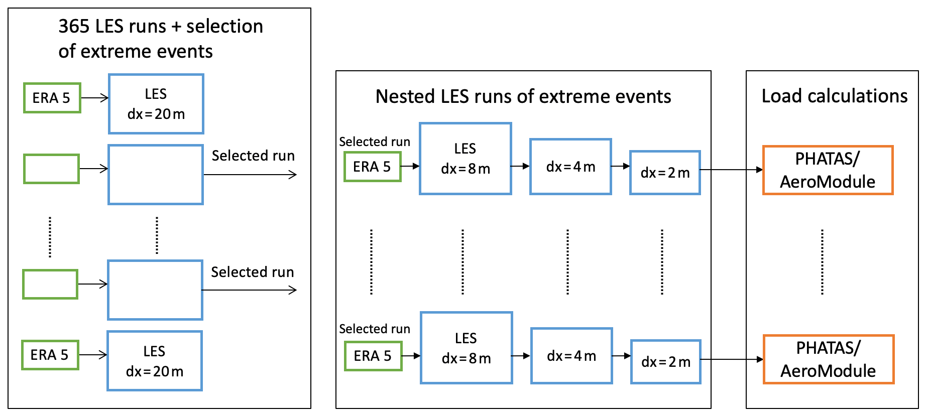
Figure 1Schematic representation of the experimental set-up. From 365 LES runs for a North Sea location, five extreme events are selected. These are re-run on higher resolution and the output passed to the aeroelastic models PHATAS and AeroModule.
The use of LES to study atmospheric flows through wind farms is gaining popularity in the scientific community. In an overview paper, Mehta et al. (2014) discuss several applications of LES in the context of wind turbine loads. One of the strengths of LES that is frequently mentioned by the papers cited in Mehta et al. (2014) is its ability to represent realistic atmospheric conditions in which aspects like shear, veer, stability and turbulence are coherently modelled. The ability of LES to realistically model complex atmospheric flows through wind farms is also stressed by Stevens and Menevau (2017), but, like Mehta et al. (2014), the authors also conclude that LES is computationally too expensive for use in wind farm design. Owing to these computational barriers, the use of LES in an operational context (e.g. for forecasting or for wind resource assessments) or in wind turbine design has so far been limited. Of particular relevance for the present paper is the work of Storey et al. (2013), who have dynamically coupled an LES model to a detailed turbine model using the FAST aeroelastic code. The two-way coupling realised by Storey et al. (2013) is not pursued in the present paper, where only the turbulent inflow fields are passed on an aeroelastic model. The main novelty that we demonstrate, however, is to move away from the stylised velocity input profiles as input for the LES model. Instead, we use the LES model GRASP (GPU-Resident Atmospheric Simulation Platform) driven by boundary conditions from a global weather model to produce a year-long simulation of the weather at the offshore met mast IJmuiden. GRASP is computationally optimised and therefore enables detailed modelling of meteorological phenomena on a spatial and temporal grid resolution which is fine enough for aeroelastic load calculations. From the yearly results, we select the five most extreme events in the following categories: shear, veer, turbulence intensity, turbulent kinetic energy and a low-level jet. Special attention will be given to the analysis of results at an extreme low-level jet, since these events are often believed to have significant impact on turbine loading; see, e.g. Duncan (2018).
The resulting extreme wind events are then fed as wind input to the aeroelastic solver PHATAS from WMC (now LM) as used by TNO Energy Transition (Lindenburg, 2005) and the aerodynamic modelling from the AeroModule tool (Boorsma et al., 2012), which offers the choice between an efficient lower-fidelity blade element momentum (BEM) method and a higher-fidelity but less efficient free vortex wake model. The turbine on which the loads are calculated is the 10 MW reference wind turbine as designed in the EU project AVATAR (Sieros et al., 2015). The calculated loads in response to these extreme wind events are compared with the loads from a reference design load spectrum which is available from the AVATAR project (Stettner et al., 2015). This reference design load spectrum is calculated according to the IEC standards. In this way it can be assessed whether the wind fields from extreme events modelled with LES yield loads that deviate significantly from the design load spectrum. A final topic of investigation is to compare the loads calculated by a model based on blade element momentum theory (BEM) with those from a higher-fidelity model: the free vortex wake model Aerodynamic Wind Turbine Simulator (AWSM) (Boorsma et al., 2012). In previous studies indications were found that BEM could overpredict loads for cases with artificial shear (Boorsma et al., 2019). The present study could confirm these findings for realistic shear cases.
The work described in the present paper can thus be seen as a proof-of-concept study to explore the merits of using high-fidelity wind simulations as input for load calculations. Such site-specific simulations could someday be done more routinely in wind turbine and wind farm design and could eventually lead to a rethinking of the use of standard design load spectra.
The article is structured in the following way: Sect. 2 provides details on the wind and turbine modelling details. Section 3 provides the results in two parts: first the wind modelling results are presented and compared with observations. This also serves as a validation of the modelled wind inputs. Secondly, the load results are presented. The comparison between the loads from the extreme events and those from the reference spectrum is given together with an evaluation of results. Conclusions and recommendations for further research are given in Sect. 5.
The overall experimental set-up of the research is depicted schematically in Fig. 1. Two series of LES runs have been performed: the first one covering the whole year to select the extreme events and the second one to run the selected cases in higher resolution. The wind fields from the selected cases have been passed to the aeroelastic model.
2.1 Location
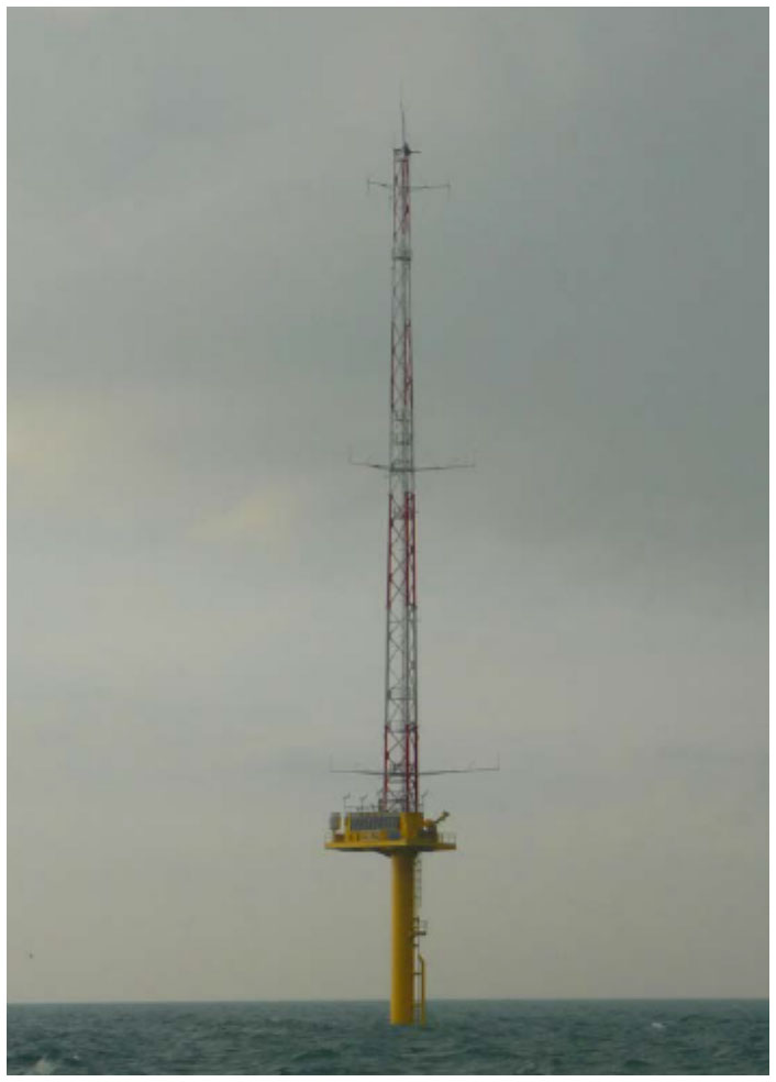
The site for which the LES runs are conducted is the location of the Meteomast IJmuiden (MMIJ) in the North Sea, 85 km offshore from the Dutch shore (52∘50.89′ N, 3∘26.14′ E). The mast is shown in Fig. 2, and the instrumentation of the mast is given in Werkhoven and Verhoef (2012). Measurements are taken with anemometers on a mast which are placed at three different heights above sea level, i.e.: 27, 58 and at the top level of 92 m (note that some wind speed sensors are mounted at an altitude of 85 m as well). They are combined with lidar measurements which are taken at 90, 115, 140, 165, 190, 215, 240, 265, 290 and 315 m a.s.l. (above sea level).
The observations from the met mast are not directly used as input for either the LES runs or the load calculations. However, the main benefit of choosing this site for our numerical study is that it allows us to do a validation of the modelled winds against observations.
2.2 LES setup
GRASP is a large-eddy simulation (LES) model developed by Whiffle that is based on the Dutch Atmospheric Large Eddy Simulation (DALES). The LES code runs on graphics processing units (GPUs) and is therefore referred to as GRASP: GPU-Resident Atmospheric Simulation Platform. GRASP can be run with boundary conditions from a large-scale weather model (Gilbert et al., 2020). For this study, GRASP has been run for the location of the Meteomast IJmuiden in the Dutch North Sea area with boundary conditions from the ERA5 reanalysis dataset (Hersbach et al., 2020) that provides global data of historical atmospheric and ocean conditions. A double periodic LES domain is used to allow full development of the turbulence. As a consequence, the ERA5 boundaries cannot be directly prescribed at the edges of the domain but are prescribed as dynamic tendencies. This means that the rate equations for the LES variables contain an extra term due to large-scale advection. For the velocity components, a second source term accounts for the large-scale pressure gradient as a driving force. More information about this set-up can be found in Schalkwijk et al. (2015). Driving the LES with boundary conditions from a large-scale weather model ensures that the full spectrum of atmospheric flow from synoptic to turbulent scales is considered. Amongst others, the interaction between atmospheric stability, turbulence, and shear is resolved.
A full year of LES runs of 24 h each (i.e. 365 simulations of 24 h, plus a 2 h spin-up period for each simulation) has been performed on a resolution of 20 m. From this year of model simulations, several types of extreme wind events have been identified, including low-level jets and high-shear, high-veer and high-turbulence cases. These cases have been re-run and used as boundary conditions for a higher-resolution run in the concurrent precursor setting. To this end, a three-way nested simulation has been carried out (see Fig. 3) at 8, 4 and 2 m resolution with 256 grid boxes in each direction which gives a domain size of 2×2 km2, 1×1 km2 and 500×500 m2 respectively. The finest grid with a resolution of 2 m yields 51 wind speed points over the 103 m AVATAR blade radius. The finest temporary resolution is 10 Hz, which yields an azimuth interval of 6∘ at the rated rotor speed of 10 rpm (which is on the order of intervals used in aeroelastic simulations). The computation time of the year of LES runs on 20m resolution amounts to roughly 2 d on a cluster with four NVIDIA Volta GPUs plus some additional runtime for the selected high-resolution runs. The chaotic character of the wind field in Fig. 3 illustrates the realistic representation of atmospheric turbulence in the model as well as the nesting settings.
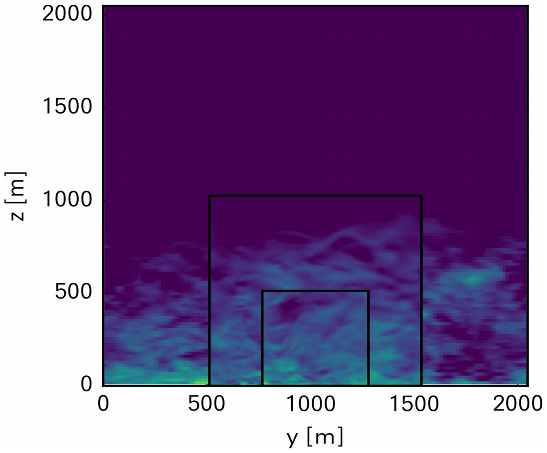
Figure 3Vertical cross sections of wind speed in the three different nested LES runs. The coarsest runs use periodic lateral boundary conditions and large-scale forcing from ERA5. The higher-resolution runs use lateral boundary conditions from the “upper” nests.
2.3 Reference turbine
The turbine that is used for the load calculations is the AVATAR reference wind turbine (RWT) (Sieros et al., 2015). This is a turbine with a rated power of 10 MW as designed in the EU project AVATAR. The AVATAR RWT is a low-induction variant of a 10 MW RWT designed from the INNWIND.EU project; see Bak et al. (2013). The main characteristics of the AVATAR RWT are listed in Table 1.
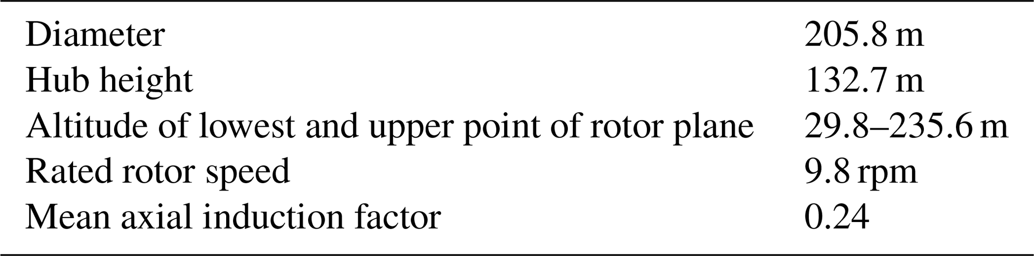
The low induction concept used in the AVATAR RWT makes an increase in rotor diameter possible from D=178 m (i.e. the diameter of the Innwind.EU RWT) to D=205.8 m with a limited increase in loads. The hub height of the AVATAR RWT is 132.7 m by which the lowest point of the rotor plane is at an altitude of 29.8 m, and the upper part of the rotor plane is at 235.6 m. The rated rotor speed is 9.8 rpm. All design data (the aerodynamic and aeroelastic data of blades, tower, shaft, and other components) of the AVATAR RWT are publicly available (Sieros et al., 2015).
A controller has been designed that covers two regimes. Below rated wind speed, the controller aims for maximum power production with variable rotor speed operation using a speed-dependent generator torque set point (for optimum tip speed ratio) and constant optimal blade pitch angle. Above rated wind speed, the rotor speed and generator power are regulated to their nominal rating using constant generator torque and collective blade pitch control.
As a reference case to compare the loads resulting from the extreme events from the LESs, a standard design load spectrum has been calculated (Stettner et al., 2015). The calculations of the design load spectrum have been repeated with the most recent versions of design tools to assure consistency in tools.
2.4 Aeroelastic modelling of extreme events
The aeroelastic loads in response to the extreme GRASP cases are calculated with the PHATAS code (Lindenburg, 2005) using two different solvers: one based on blade element momentum (BEM) theory and one based on the free vortex wake model. The development of the PHATAS code started in 1985 by ECN (now TNO), but later the code was transferred to WMC (now LM). The code takes into account blade flexibilities in all three directions (flatwise, edgewise and torsional) but also tower and drivetrain flexibilities. Furthermore, the control of the AVATAR turbine as described in Sect. 2.3 is taken into account.
The default aerodynamic solver of PHATAS is based on blade element momentum (BEM) theory. This is an efficient but lower-fidelity model, which, because of its efficiency, is used for industrial design calculations. In its basis a BEM model is steady and 2D, by which phenomena like yaw and stall are calculated with a very large uncertainty. Therefore, in the last decades several engineering models have been developed which are added to the BEM theory. These engineering add-ons cover phenomena like unsteady and 3D effects as well as yaw and stall. They are still of a simplified efficient nature, which makes them suitable for industrial calculations. These engineering models are validated and improved with the most advanced measurement data (Schepers, 2012) and with high-fidelity models (Schepers, 2018).
The GRASP events are calculated with a PHATAS version which is linked to an alternative aerodynamic solver AeroModule as developed by TNO. AeroModule is a code which has an easy switch between an efficient BEM-based model and a high-fidelity but time-consuming free-vortex-wake-based model AWSM (Boorsma et al., 2012). This allows for a straightforward comparison of these two models with precisely the same input. In this way it can be assessed how well the load response is calculated with a BEM model in comparison to the load response as calculated from the higher-fidelity model AWSM.
In the present study the blade root flatwise moment is considered. Both extreme loads and the damage-equivalent fatigue loads (DELs) are considered where the latter is based on a Wohler slope of 10. It is noted that the damage equivalent load translates the underlying rain flow cycle spectrum into a single number. This facilitates the presentation of results, but it conceals the underlying frequency information from the rain flow cycle spectrum. The loads are calculated in the coordinate system from Germanischer Lloyd.
The computation time of the load calculations is much faster than real time for BEM on a simple laptop. The free vortex wake calculations are a factor of 100–1000 slower (dependent on number of wake points and the wake cut-off length).
2.5 Interface between GRASP and PHATAS
The input for AeroModule (and so PHATAS) consists amongst others of the 3D wind speeds at several locations in the rotor plane as a function of time. For the present study they were supplied by Whiffle in separate files in NetCDF format in the resolution which is given in Sect. 4.1.1. They were transformed by the ECN part of TNO into TurbSim wind simulator files (Jonkman, 2009). The turbine yaw angle is fixed and aligned with the time-averaged wind direction at hub height from the GRASP wind input.
2.6 Calculation of reference design load spectrum
The reference design load spectrum for the AVATAR RWT has been calculated and assessed in Stettner et al. (2015). It is calculated along the IEC standards for wind class IA, which was considered representative for offshore conditions by the AVATAR consortium. As mentioned before, this is a conservative turbulence class for the present location.
The load spectrum from Stettner et al. (2015) covers normal production (DLC 1.2), standstill, stops, etc. In the present study it is only the normal production cases from DLC 1.2 which are repeated. In Sect. 6 it will be shown that these cases are sufficient for the present assessment, and there is no need to include special cases.
The reference load cases are carried out as 10 min time series for mean wind speeds ranging from 5–25 m s−1, with a wind speed interval of 2 m s−1 and a shear exponent of 0.2, where the wind input is generated from the stochastic wind simulator SWIFT using six different seeds. A small yaw angle of 8∘ is included to account for yaw control tracking errors.
It is noted that the aerodynamic model with which the reference spectrum is calculated is based on the default BEM model of PHATAS where the GRASP events from section 4 are calculated with both BEM and free vortex wake (FVW). Apart from fundamental model differences between BEM and FVW, all calculations are carried out in exactly the same way, with the same degrees of freedom, engineering models used, etc., in order to assure consistency in results.
3.1 LES wind output
The GRASP simulations were carried out from 1 December 2014 to 1 December 2015. Figure 2 presents a comparison between modelled and observed 92 m wind speed for the entire year in the form of a scatter density plot. The agreement between the modelled and observed 92 m wind speeds is good, and no clear bias is observed. A more elaborate comparison of the yearly LES results against the MMIJ observations could provide additional insights into the performance of the LES model for specific atmospheric conditions, but this is not pursued in this paper. A more in-depth comparison of LES winds against North Sea observations is presented in Wiegant and Verzijlbergh (2019). However, in Sect. 3.2 the yearly LES results are analysed in light of their correspondence with observed turbulence, extreme shear, extreme veer and low-level jets.

From the yearly LES data, the following five “extreme” cases of 10 min were selected:
-
strongest low-level jet (LLJ) (the LLJs were detected with the algorithm from Baas et al., 2009),
-
strongest wind veer over the rotor,
-
strongest shear over the rotor,
-
highest turbulence kinetic energy (TKE) below cut-out wind speed,
-
highest turbulence intensity (TI) around rated wind speed (i.e. higher than 10 m s−1) and lower than cut-out.
For each of these five selected cases, a threefold nested simulation was performed with a spatial resolution of 2 m and a temporary resolution of 0.1 s for the finest nest. Figure 5 presents an overview of the selected extreme wind cases. For each extreme wind case (columns), profiles of wind speed (U), wind direction (ϕ), turbulence intensity (TI) and turbulent kinetic energy (TKE) are shown (rows). For comparison, the MMIJ observations and ERA5 reanalysis data are also added. Although ERA5 profiles have not been used further in the analysis, showing their profiles together with the LES profiles gives an indication of how different representation of turbulent transport in the LES model leads to different vertical wind speed profiles. Although the significance of a one-to-one comparison of modelled and observed 10 min records is limited, especially when considering extreme events, clear correspondence between the model results and the observations is observed. In Sect. 4.1.3 the modelled extreme events are discussed from a climatological point of view.
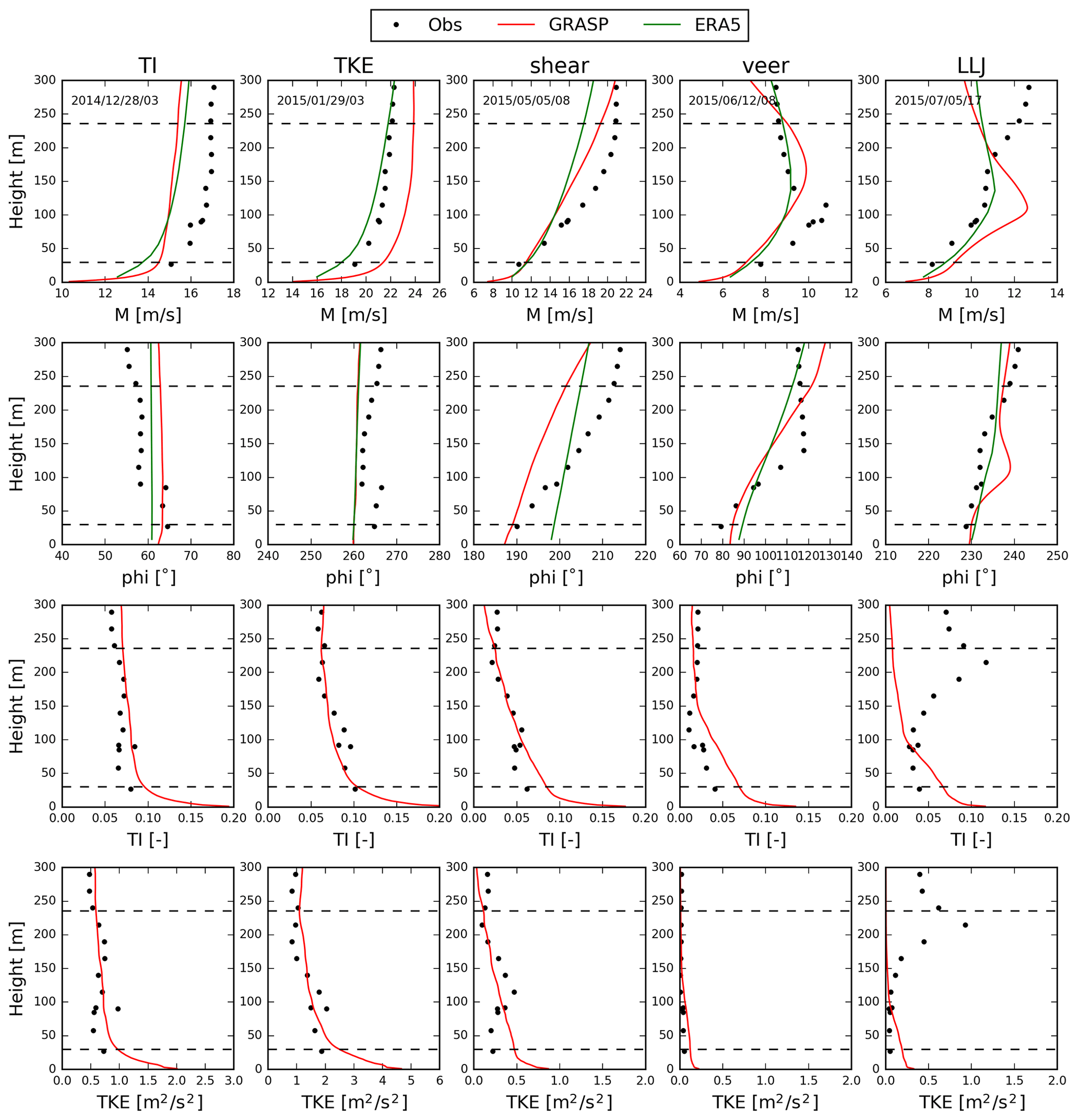
Figure 5Profiles of four meteorological quantities (wind speed U, wind direction ϕ, turbulence intensity TI and turbulent kinetic energy TKE) for the five selected extreme cases (different columns) with high TI, TKE, wind shear, veering and a strong LLJ. Observations are indicated as black dots, the high-resolution GRASP (2 m grid-spacing) results in red and ERA5 reanalysis data in green. Dashed lines indicate the upper and lower parts of the rotor plain.
For the strongest low-level jet, Fig. 4 shows that the wind speed at the lowest point of the rotor plane is approximately 9.2 m s−1 and then increases to a maximum value of almost 13 m s−1. This value is reached slightly below hub height. Above hub height the wind speed decreases to approximately 10.3 m s−1 at the upper part of the rotor plane. The wind speed variation with height goes together with a relatively large veer from approximately 230∘ at the lowest point of the rotor plane to 239∘ slightly below hub height, above which it remains more or less constant. It must be noted that a shear exponent of 0.2 (i.e. the exponent used in the IEC reference load spectrum; see Sect. 5) at a comparable hub height wind speed of 13 m s−1 yields a velocity of 9.7 m s−1 at the lower part of the rotor plane. In other words, the shear prescribed by the standards is only slightly less than the shear from the LLJ in the lower part of the rotor plane. For the selected LLJ case the corresponding observed wind profile does not show a jet-like profile. In Sect. 4.1.3 it will be shown that on a climatological basis modelled and observed low-level jets have similar characteristics.
The strongest wind veer case shows a wind direction of approximately 85∘ at the lowest part of the rotor plane and a wind direction of approximately 120∘ at the upper part, leading to a wind direction difference of 35∘. The correspondence with observations is reasonable. Note that for this strong veer case the observed and modelled wind speed profiles show a clear LLJ.
The strongest shear case shows a wind speed of approximately 11.5 m s−1 at the lowest part of the rotor plane above which it increases to almost 16 m s−1 at hub height above which it increases further to approximately 19 m s−1 at the upper position of the rotor plane. The observations show a comparable wind shear. We selected the largest wind speed difference over the rotor plane, which turned out to be 8.5 m s−1. Again, it must be noted that a wind shear exponent of 0.2 (i.e. the exponent prescribed in the standards for the normal operating condition cases) and a hub height wind speed of 16 m s−1 already give a wind speed difference of 6.2 m s−1 over the rotor plane.
For the case with extreme turbulence intensity and extreme turbulent kinetic energy, the turbulence intensities at hub height are found to be approximately 5 % and 6.5 % at approximately 14.8 and 22.5 m s−1 respectively. Although these turbulence intensities are the highest for the selected year, they are much lower than the values for turbulence class A at the corresponding wind speeds (approximately 18 % and 16 %). This indicates that the reference design load spectrum as calculated in the AVATAR project is conservative for isolated turbines at the selected site. However even a turbulence class C (the lowest possible turbulence class in IEC) leads to turbulence intensities which are still far above the extreme turbulence intensities in the selected year.
It is also important to note that the extreme shear and extreme low-level jet cases go together with very low turbulence levels. This is shown in Table 2, which gives the turbulence intensity as a function of height for the LLJ event.
Table 2Turbulence intensity as a function of height for the extreme low-level jet case.

The turbulence intensity at hub height is 1.6 %. This low turbulence intensity should be kept in mind when analysing the load results. The turbulence intensity decreases from 1.6 % at hub height to 1.2 % at h=235 m despite the decreasing wind speed above hub height in Fig. 2. This implies that the decreasing turbulence intensity with height should be attributed to a strong decrease in standard deviation of wind speed fluctuations which overcompensates for the decreasing wind speed. In fact, this is what can be expected under the strongly stratified conditions that favour the formation of LLJs. In contrast, for the LLJ case the observed values of TI do increase with height, which would be much harder to explain. Note that estimating turbulence quantities from lidar observations is not trivial; see, e.g. Sathe et al. (2011).
3.2 Climatology of extreme events
Instead of a one-to-one comparison of isolated 10 min records, here we compare the climatology of extreme wind events from the yearly GRASP LES results and the observations. Figure 6 shows profiles of wind speed and veering with height for the 90th percentile of strongest shear and veer conditions between 215 and 90 m. For strong shear conditions (left) the GRASP and ERA5 wind speed profiles are close to the observations. For these cases the wind direction changes only weakly with height and is slightly larger in the observations than in the model. For strong veer conditions (right) the wind speed is weak and constant with height above roughly 90 m. The strong veering of the wind with height is well-represented by GRASP and underestimated by ERA5. This is clearly an example where the different representation of turbulent mixing in an LES model compared to a numerical weather prediction (NWP) model leads to a different wind speed profile.
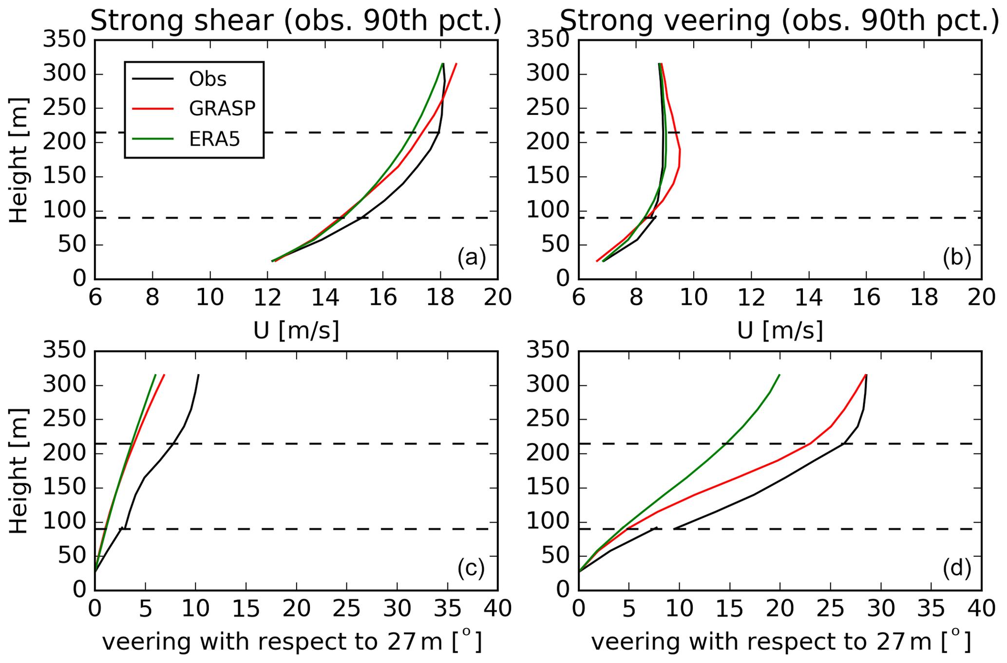
Figure 6Comparison of the 90th percentile strongest shear (a, c) and veer (b, d) conditions from observations, ERA5 and GRASP.
In Fig. 7 the standard deviation of the wind is plotted versus the wind speed for the 92 m level. The top panels include 1 year of observations and simulations. The division of these two quantities gives the TI. For reference, lines of equal TI of 5 % and 10 % are indicated. Clearly, stronger winds yield more intense fluctuations. The model tends to have slightly higher TI values than observed, but the difference is within a few percent. For wind speeds of around 10 m s−1, the observed and modelled TI values are mostly close to 5 %.
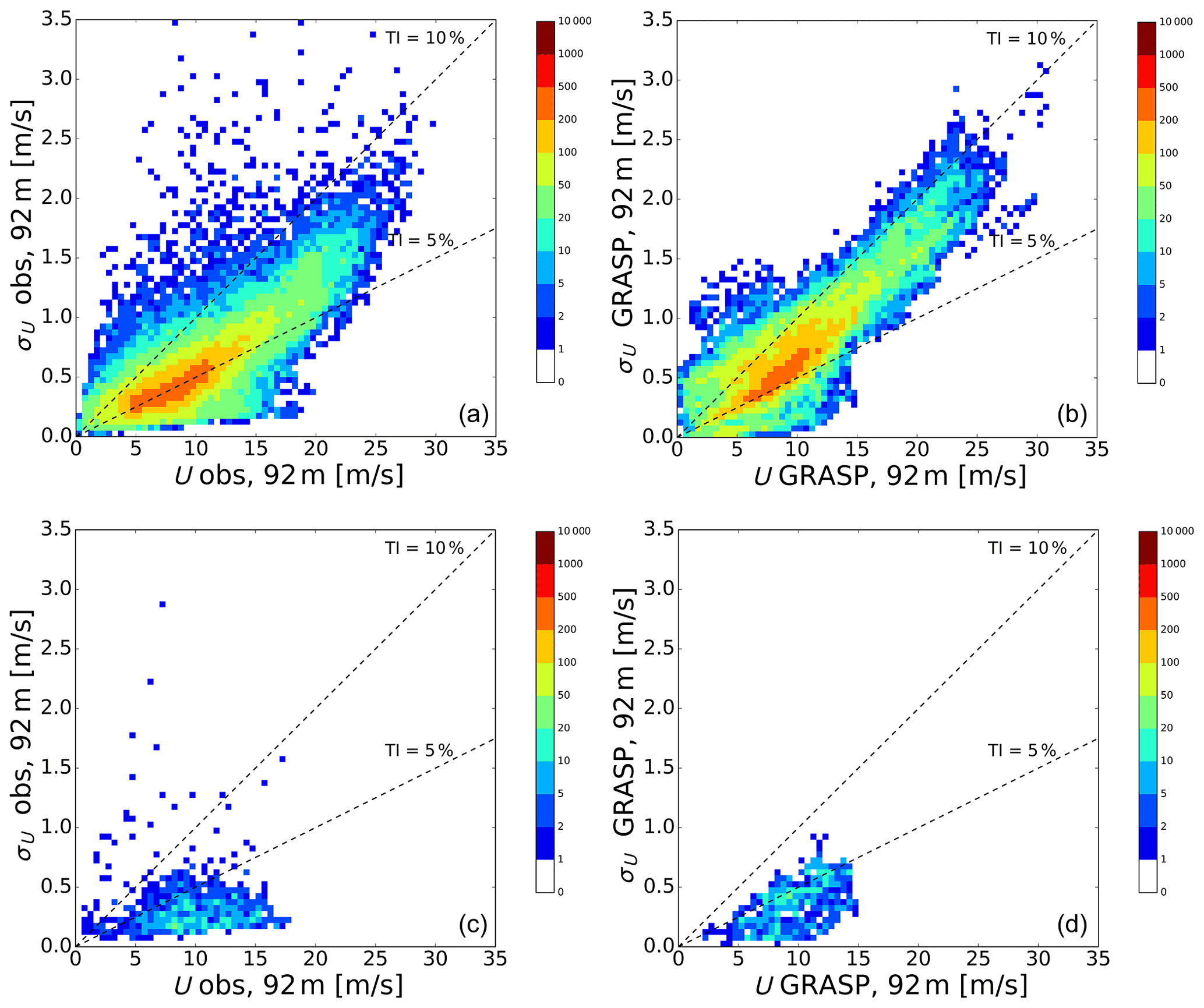
Figure 7Scatter–density plot of the standard deviation of the wind speed versus the wind speed at the 92 m level. (a, c) Observations; (b, d) model results; (a, b) entire year; (c, d) only LLJ cases.
In Sect. 6 of this paper, it will be shown that the loads from the LLJ are relatively low. The low loads at LLJ are partly caused by the very low turbulence intensities which go together with an LLJ. This raises the question of whether these low turbulence intensities at LLJs are also found in the measurements. Therefore, the lower panels of Fig. 7 only include data points that satisfy the criterion for the occurrence of a low-level jet. In both the observations and the LES results, the TI values of LLJ events are generally in the range of 2 % (sometimes even less than 1 %) at an altitude of 92 m. This can be seen as a confirmation that such low turbulence intensities are found at LLJ events and are well represented by the LES model.
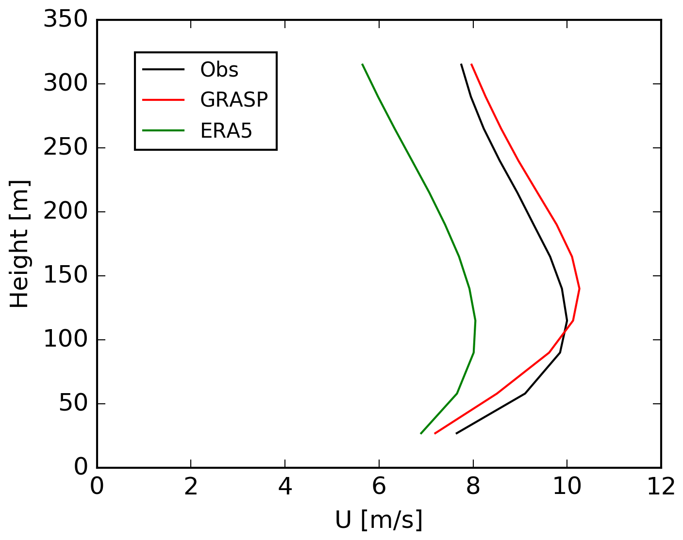
Figure 8 shows average low-level jet wind speed profiles for the observations, GRASP and ERA5, i.e. the profiles averaged over all timestamps of the respective dataset when a LLJ was present according to the LLJ criterion (Baas et al., 2009). The agreement between GRASP and the observations is within roughly 0.5 m s−1, whereas ERA5 underestimates the speed of the LLJ by approximately 2 m s−1. The frequency of LLJ occurrence is highest in the observations with 4.8 % of the 10 min records. For GRASP and ERA5 the LLJ frequency amounts to 2.3 % and 0.6 % respectively.
Concluding remarks on wind validation
In summary, the extreme wind cases that were selected based on GRASP model output represent “real weather”. That is to say, there is a strong qualitative and often quantitative agreement between the modelled and observed extreme events of LLJ, wind shear, veer, TI and TKE. Although the agreement for the selected LLJ is moderate, it is encouraging to see that many other LLJ events in the year of simulation find a shear which is comparable to the measurements. Moreover, most LLJs go together with low turbulence levels and large veer in both calculations and measurements. In general, the climatology of the extreme events (shear, veer, TI, turbulent kinetic energy (TKI) and LLJ) as modelled by GRASP resembles the observed extreme events well.
3.3 Comparison between aeroelastic loads at extreme events with loads from the reference spectrum
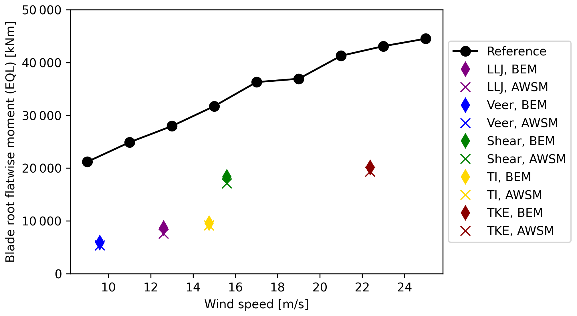
Figure 9 shows the resulting equivalent fatigue flatwise moment as a function of the 10 min averaged wind speed from the reference design load spectrum and extreme GRASP events. The values indicated with reference are the loads as calculated for DLC 1.2. They are compared with the BEM- and AWSM-calculated loads for the case of extreme low-level jet (LLJ), veer, shear, turbulence intensity (TI) and turbulence kinetic energy (TKE).
In Fig. 10, the extreme flatwise moment as extracted from the 10 min time series is compared and again plotted as a function of wind speed. The extreme load has been extracted for a BEM-based calculation only. The presentation of extreme loads as a function of wind speed may not be the most relevant metric for design purposes, since it is the overall maximum value which determines the design. This way of presenting is chosen because it shows the wind speeds where the extreme events are found. In all cases the extremes were found to be the maximum positive values (using the sign conventions from the Germanischer Loyd (GL) coordinate system). The design load spectrum has been calculated for six different seeds per wind speed. The results from Fig. 9 are based on the averaged equivalent load. The values from Fig. 10 are the overall extremes per wind speed.
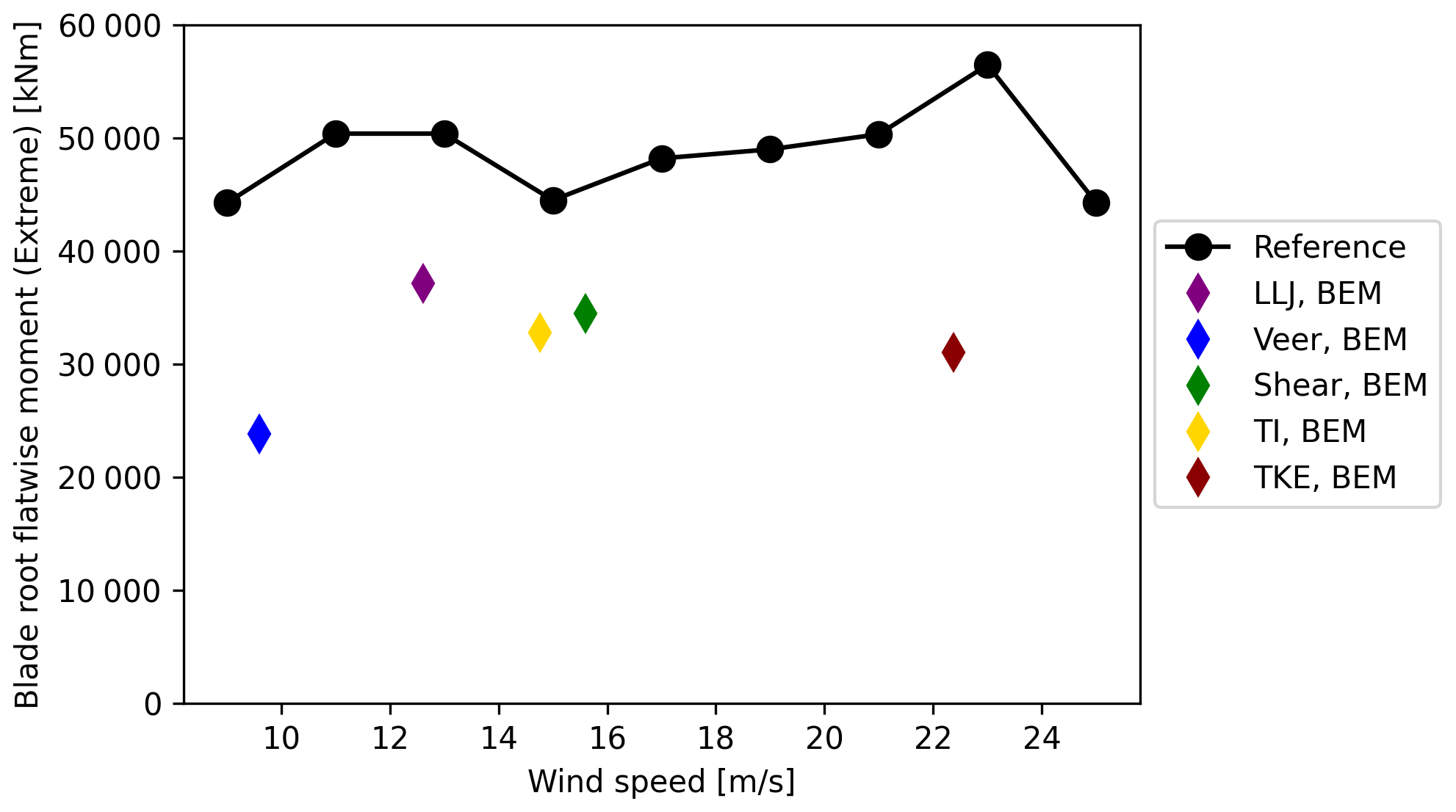
The present analysis is based on normal production cases (DLC 1.2), which means that special and extreme load cases are excluded. As such the actual maximum extreme load from a full IEC spectrum could even be higher than the values presented in Fig. 10. Some indication for that is found in Savenije et al. (2017), which shows that often non-DLC 1.2 cases (e.g. DLC 6.2, idling at storm loads) are more extreme indeed.
In order to gain some further understanding of the results, the loads from the low-level jet are analysed in more detail. Table 3 compares the DEL of the flatwise moment from DLC 1.2 at 13 m s−1 (second row) with those from the low-level jet as calculated with BEM (third row) and AWSM (fourth row). Note that the wind speed of 13 m s−1 is very close to the 10 min averaged hub height wind speed at the low-level jet. In the second column the DEL of the full load is calculated, which corresponds to the results from Fig. 9.
Table 3Comparison of equivalent blade root flatwise moment for extreme low-level jet (relative to the DEL of DLC 1.2).
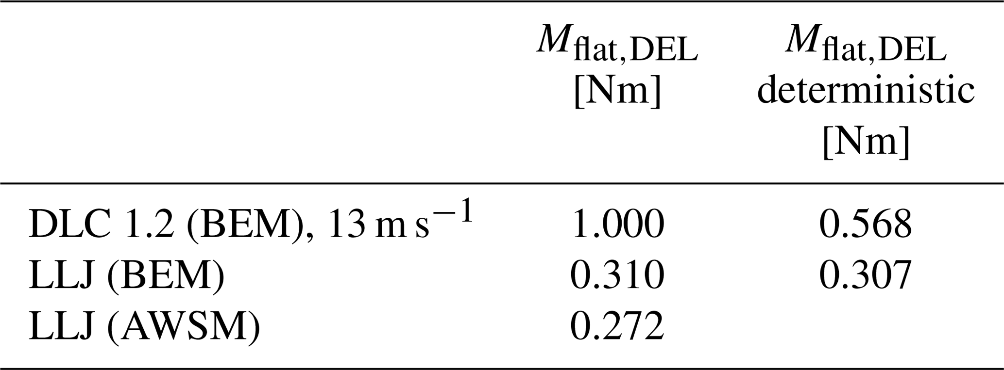
The third column gives the DEL from the azimuthally binned averaged variation. This azimuthally binned averaged variation is (for a linear system) similar to the deterministic variation which is mainly a result of the shear (although the veer in the LLJ event and the 8∘ yaw error for DLC 1.2 lead to a deterministic variation as well). The equivalent loads from the deterministic variation are calculated for the BEM results only. All DELs are normalised with those from the full load of DLC 1.2.
3.3.1 Assessment of loads from extreme events
An important observation is that the loads in response to the extreme wind events from GRASP remain within the load envelope of the reference spectrum. This is true for the equivalent fatigue loads (see Fig. 9), which shows that all DELs from the GRASP extreme events are lower than the DELs from the reference DLC 1.2 at comparable wind speeds. It is also true for the extreme loads; see Fig. 10. As explained above, the “real” extreme reference loads are likely to be even higher than the values given in these figures, since the results in these figures consider DLC 1.2 only. This makes the extreme loads from the GRASP wind events remain within the reference spectrum within an ever wider margin.
From Table 2 it can be concluded that the equivalent flatwise moment at the LLJ is only 31 % (approximately) of the equivalent load from DLC 1.2. The modelled wind profiles and turbulence levels during the LLJ events provide some further insights into this. As mentioned in Sect. 4.1.2 the turbulence level at the low-level jet is extremely low (approximately 1.6 % at hub height) where the turbulence level for DLC 1.2 at 13 m s−1 is on the order of 19 %. The very low turbulence level at the LLJ explains, at least partly, the much lower fatigue load. This is confirmed by the DEL of the deterministic variation in the third column which is almost similar (99 %) to the DEL of the total variation in the first column. The 1 % difference is the addition from turbulence and should be compared with the difference between deterministic and total variation from DLC 1.2, which is approximately 43 %. This indicates how little the low turbulence level at the LLJ adds to the fatigue loads.
Still the DEL of the deterministic variation at the LLJ is much lower (approximately 54 %) than the DEL of the deterministic variation at DLC 1.2. This indicates that the low fatigue loads at a LLJ are not only caused by the lower turbulence level, but it is also the different shear from the LLJ which lowers the DEL. Some further explanation is offered by Fig. 11, which shows a comparison between the azimuthally binned averaged flatwise moments for the LLJ and DLC 1.2. Azimuth angle zero indicates the 12 o'clock position. The rotor rotates clockwise so azimuth angle 90 indicates the 3 o'clock position when looking to the rotor. The variation from DLC 1.2 has a 1P variation with a relatively large amplitude. This is the behaviour of the flatwise moment in an atmosphere with “common” vertical wind shear. The wind speed (and so the loads) decreases when the blade rotates from the vertical upward 12 o'clock (zero azimuth) position to the vertical downward 6 o'clock (180 azimuth). The flatwise moment increases again when the blade rotates from 180∘ towards 360∘.
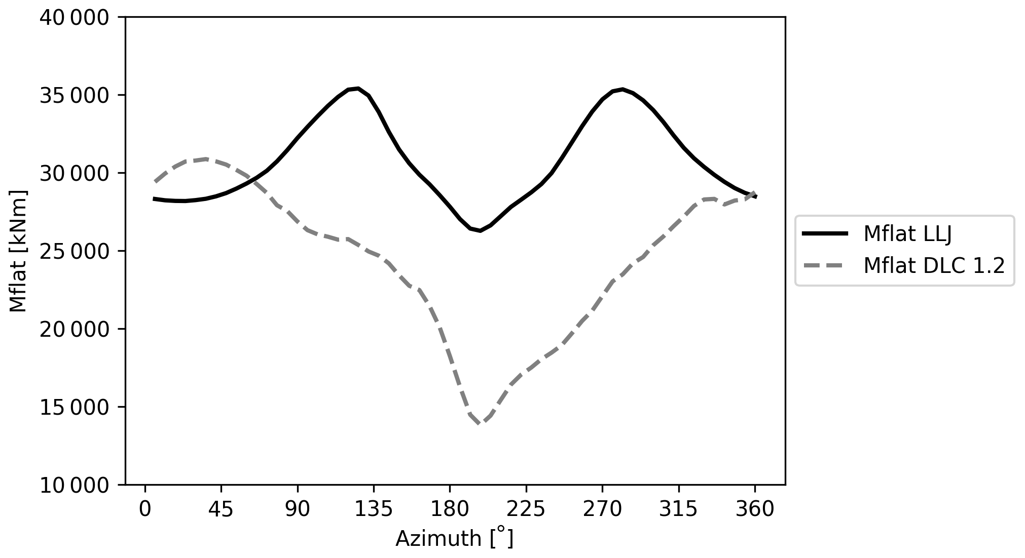
The azimuthal variation in flatwise moment from the low-level jet is very different from the variation which results from DLC 1.2. It shows a 2P variation with a relatively small amplitude. This 2P variation can be explained with the LLJ wind speed profile from Fig. 5 which shows the wind speed to be low at 0∘ azimuth (the 12 o'clock position, when the blade is pointing vertically upward) and at 180∘ (the 6 o'clock position, when the blade is pointing vertically downward). The wind speed is maximum at (approximately) hub height which corresponds to azimuth angles of 90 and 270∘ (i.e. the 3 and 9 o'clock positions when the blade is standing horizontally). This velocity variation is reflected in the flatwise moment. It is low at 0∘, high at (roughly) 90 and 270∘, and low again at 180∘. This leads to a 2P variation, but the load amplitude is relatively small. Hence, although the 2P load variation happens twice as often as the 1P load variation from the DLC 1.2, the lower amplitude of the variations leads to a lower fatigue.
It is noted from Fig. 5 that the present LLJ has a maximum velocity close to hub height, and it could be argued that a different hub height leads to a different load behaviour. The lowest part of the rotor plane of the AVATAR RWT is at an altitude of 29.8 m, and the upper part is at an altitude of 235.6 m. It was not considered feasible to decrease the tower height and lower the rotor plane even more. Also, a lowering of hub height would bring the maximum in LLJ wind speed even closer to hub height (see Fig. 4). Therefore, an increase in tower height has been investigated, but this was limited by the domain size of the GRASP field which extends up to a maximum altitude of 255 m. Hence the tower height cannot increase with more than 19.4 m. A hub height of 250.7 m has been investigated, but this did not lead to significantly different conclusions (i.e. the loads from the LLJ remain within those of the reference spectrum). Alternatively, a LLJ event that has its wind maximum at a different height (e.g. at the top of the rotor plane) could lead to a markedly different load behaviour.
3.3.2 Accuracy of calculating loads from extreme events
From Fig. 9 and Table 3 it can be concluded that the DEL of the blade root flatwise moment is overpredicted with the BEM model (assuming that the fatigue loads as calculated with the FVW model AWSM are close to reality). Similar observations were made in Boorsma et al. (2016, 2019) where differences are reported on the order of 10 %–20 % for load cases which are representative of IEC normal production. The present study shows overpredictions which are on the same order of magnitude, i.e. 14 % for the extreme LLJ, 11 % for the extreme veer case, 7 % for the extreme shear case but only 4 %–5 % for the extreme turbulence intensity and turbulent kinetic energy. The difference between AWSM- and BEM-based fatigue shaft loads (not shown in this paper) was generally found to be smaller and less straightforward than for the blade root flatwise moment: in some cases, AWSM even predicts higher fatigue loads than BEM.
The commonly believed explanation for the overpredicted BEM DEL lies in a more local tracking of the induced velocity variations in FVW models, by which they vary synchronously with the variation in inflow. This synchronisation then damps out the variations in angle of attack. It should then be noted that the AVATAR RWT is a low induction concept, i.e. a concept which is less sensitive to such induction-driven phenomena. This makes it plausible that the difference for conventional turbines with higher induction is even larger. Moreover, FVW models allow for a more intrinsic and realistic modelling of shed vorticity variations in time.
This paper has described a study in which turbulent wind fields generated with LES were passed to the aeroelastic code PHATAS (with AeroModule) from the ECN part of TNO. The wind fields corresponded to extreme events selected from a 1-year simulation of the LES wind fields. These events are fed as wind input files to the PHATAS code and used to simulate the AVATAR 10 MW reference wind turbine (RWT) at an offshore location.
A validation of the LES wind fields has taken place by comparing the calculations with measurements from Meteomast IJmuiden. This validation shows that there is generally a good agreement in the load-determining characteristics of the LES wind fields by which the calculated events can be used with confidence to assess the importance of them in an aeroelastic load context. However, more validation is needed, in particular on turbulence characteristics at high altitudes (say higher than 100 m).
The resulting (DEL and extreme) loads for the selected events are (roughly speaking) 30 %–70 % lower than those from the reference design load spectrum of the AVATAR RWT. As such, the often-heard expectation that low-level jets have a significant impact on loads is not confirmed for the present offshore situation. This is partly explained by the low turbulence intensities (roughly 1 %–2 %) which go together with the LLJ. However, the deterministic DEL from the LLJ shear is also lower than the deterministic DEL from DLC 1.2. This is due to the fact that the shear from the LLJ is not extreme in comparison to the shear from the IEC standards. The LLJ shear profile then leads to a 2P variation instead of a 1P variation from “normal shear”, but the amplitude is smaller, resulting in a lower fatigue damage. From the results one could hypothesise that the combination of the shear and turbulence levels from the IEC standards may often lead to conservative loads. However, more research is needed to warrant a conclusion, especially in the validation of the on-site turbulent wind fields.
It is noted that the present LLJ has, more or less by coincidence, a maximum velocity close to hub height. A study on different hub heights did not show a very different outcome, but the limited domain size of the LES wind field made it so that the hub height could not increase more than 20 m. A study with a much taller tower (and so an extended domain size) is recommended.
For the selected extreme events, the DEL from the more physical AWSM model is considerably lower than the DEL of the BEM model, which indicates that BEM overpredicts fatigue loads. The difference is largest for the shear-driven cases and for a rigid construction. Efforts should be undertaken to improve the BEM fatigue calculations for such shear events.
The present research can be considered a proof-of-concept study to investigate the potential coupling between turbine response models and high-fidelity wind models. The demonstrated computational feasibility and the results lead to the recommendation to explore such coupling even further for the calculation of a full design load spectrum. This makes it possible to assess the validity of a conventional method for the calculation of a design load spectrum based on stochastic wind simulators. The higher fidelity of the present method makes it so that eventually design calculations could be based on physical wind models. Future work should focus on applying and validating this method in more challenging case studies, such as in full-scale wind farms where the down-stream turbulence is heavily affected by the turbines themselves. Including other wind turbines in the LES domain also has the benefit that the implicit assumption that the upstream turbulence is not affected by the turbine can be overcome. Finally, we recommend also studying situations where turbines are situated in complex terrain environments.
Although the coupling between PHATAS and GRASP was proven feasible, the interfacing through GRASP output and PHATAS wind input files can be improved. Ideally an on-line coupling should be developed without the need of interface files. This would also enable a two-way coupling, where force components and blade positions are passed back to the LES model during run-time.
| BEM | Blade element momentum |
| DEL | Damage equivalent load |
| DOWA | Dutch Offshore Wind Atlas |
| FVW | Free vortex wake |
| RWT | Reference wind turbine |
| TKE | Turbulent kinetic energy |
| TI | Turbulent intensity |
| LLJ | low-level jet |
The AeroModule code is available through a license at TNO. GRASP is a commercial large-eddy simulation code and is not publicly accessible.
The datasets used in this article are available upon request.
GS assembled and ran the load simulation results and analysed the overall results. PvD and HJ modified the LES code and performed the GRASP simulations. RV assisted in the analysis of the results. PB performed the validation of the GRASP simulations.
The authors declare that they have no conflict of interest.
Publisher's note: Copernicus Publications remains neutral with regard to jurisdictional claims in published maps and institutional affiliations.
This article is part of the special issue “Wind Energy Science Conference 2019”. It is a result of the Wind Energy Science Conference 2019, Cork, Ireland, 17–20 June 2019.
The research was carried out within the Dutch national project DOWA sponsored by the Topsector Energy Subsidy from the Ministry of Economic Affairs and Climate. Feike Savenije (ECN part of TNO) is acknowledged for the calculation of the reference load spectrum. Koen Boorsma (ECN part of TNO) is acknowledged for his support on the AeroModule code.
This research has been supported by the Topsector Energy Subsidy from the Dutch Ministry of Economic Affairs and Climate (grant no. TEHE117003).
This paper was edited by Katherine Dykes and reviewed by Pietro Bortolotti and David Verelst.
Baas, P., Bosveld, F. C., Klein Baltink, H., and Holtslag, A. A. M.: A climatology of nocturnal low-level jets at Cabauw, J. Appl. Meteorol. Clim., 48, 1627–1642, 2009.
Bak, C., Zahle, F., Bitsche, R., Kim, T., Yde, A., Henriksen, L. C., Hansen, M. H., Blasques, J. P. A. A., Gaunaa, M., and Natarajan, A.: The DTU 10 MW Reference Wind Turbine, Danish Technical University, Lyngby, Denmark, 2013.
Boorsma, K., Grasso, F., & Holierhoek, J. Enhanced approach for simulation of rotor aerodynamic loads. Energy Research Center of the Netherlands, ECN-M-12-003, 2012.
Boorsma, K., Chasapogianis, P., Manolas, D., Stettner, M., and Reijerkerk, M.: Comparison of models with respect to fatigue load analysis of the INNWIND.EU and the AVATAR RWT, Deliverable D4.6 of the EU project AVATAR, TNO Energy Transition, Petten, the Netherlands, 2016.
Boorsma, K., Wenz, F., Aman, M., Lindenburg, C., and Kloosterman, M.: TKI WOZ VortexLoads final report, TNO 2019 R11388, TNO Energy Transition, Petten, the Netherlands, 2019.
Duncan, J.: Observational Analyses of the North Sea low-level jet, TNO R11428, TNO Energy Transition, Petten, the Netherlands, 2018.
Gilbert, C., Messner, J. W., Pinson, P., Trombe, P. J., Verzijlbergh, R., van Dorp, P., and Jonker, H.: Statistical post-processing of turbulence-resolving weather forecasts for offshore wind power forecasting, Wind Energy, 23, 884–897, https://doi.org/10.1002/we.2456, 2020.
Hersbach, H., Bell, B., Berrisford, P., Hirahara, S., Horányi, A., Muñoz-Sabater, J., Nicolas, J., Peubey, C., Radu, R., Schepers, D., Simmons, A., Soci, C., Abdalla, S., Abellan, X., Balsamo, G., Bechtold, P., Biavati, G., Bidlot, J., Bonavita, M., De Chiara, G., Dahlgren, P., Dee, D., Diamantakis, M., Dragani, R., Flemming, J., Forbes, R., Fuentes, M., Geer, A., Haimberger, L., Healy, S., Hogan, R. J., Hólm, E., Janisková, M, Keeley, S., Laloyaux, P., Lopez, P., Lupu, C., Radnoti, G., de Rosnay, P., Rozum, I., Vamborg, F., Villaume, S., and Thépaut, J. N.: The ERA5 global reanalysis, Q. J. Roy. Meteorol. Soc., 146, 1999–2049, https://doi.org/10.1002/qj.3803, 2020.
Jonkman, B.: TurbSim User Guide, NREL/TP-500-46198, NREL, Boulder, USA, 2009.
Lindenburg, C.: PHATAS Program for Horizontal Axis Turbine Analysis and Simulation, ECN-I-05-005, ECN – Energy Research Center of the Netherlands, Petten, the Netherlands, 2005.
Mann, J.: Wind field simulation, Probab. Eng. Mech., 13, 269–282, 1998.
Mehta, D., van Zuijlen, A. H., Koren, B., Holierhoek, J. G., and Bijl, H.: Large Eddy Simulation of wind farm aerodynamics: A review, J. Wind Eng. Indust. Aerodynam., 133, 1–17, https://doi.org/10.1016/j.jweia.2014.07.002, 2014.
Sathe, A., Gotschall, J., and Courtney, M.: Can Wind Lidars measure turbulence, J. Atmos. Ocean. Tech., 28, 853–868, https://doi.org/10.1175/JTECH-D-10-05004.1 , 2011.
Savenije, F., Gonzalez Salcedo, A., Martin San Roman, R., Lampropoulos, N., Barlas, A., Sieros, G., Prospathopoulos, J., Manolas, D., Sartori, L., Jost, E., and Maeder, T.: Evaluation of the new design, The advanced Reference Wind Turbine, Deliverable 1.7 of the EU project AVATAR, TNO Energy Transition, Petten, the Netherlands, 2017.
Schalkwijk, J., Jonker, H. J. J., Siebesma, A. P., and Bosveld, F. C.: A Year-Long Large-Eddy Simulation of the Weather over Cabauw: an Overview, Mon. Weather Rev., 143, 828–844, https://doi.org/10.1175/MWR-D-14-00293.1, 2015.
Schepers, J. G.: Engineering models in Wind Energy Aerodynamics, PhD thesis, TU Delft, Delft, November 2012.
Schepers, J. G.: Final Report of the EU project AVATAR, available at: http://www.eera-avatar.eu/fileadmin/avatar/user/AVATAR_final_report_v26_2_2018.pdf (last access: 17 December 2019), 2018.
Sieros, G., Lekou, D., Chortis, D., Chaviaropoulos, P., Munduate, X., Irissarri, A., Madsen, H. A., Yde, K., Thomsen, K., Stettner, M., Reijerkerk, M., Grasso, F., Savenije, R., Schepers, G., and Andersen, C. F.: Design of the AVATAR RWT rotor, Deliverable D1.2 of the EU project AVATAR, TNO Energy Transition, Petten the Netherlands, 2015.
Stettner, M., Reijerkerk, H. J., Kooijman, A., Irisarri Ruiz, H. A., Madsen, D. R., Verelst, A., Croce, L., Sartori, M. S., Lunghini, M.: Evaluation and cross-comparison of te AVATAR and INNWIND.EU RWT's, Deliverable D1.3 of EU project AVATAR, TNO Energy Transition, Petten the Netherlands, 2015.
Stevens, R. J. A. M. and Meneveau, C.: Flow structure and turbulence in wind farms, Annu. Rev. Fluid Mech., 49, 311–339, 2017.
Storey, R. C., Norris, S. E., Stol, K. A., and Cater, J. E.: Large eddy simulation of dynamically controlled wind turbines in an offshore environment, Wind Energy, 16, 845–864, https://doi.org/10.1002/we.1525, 2013.
Veers, P., Dykes, K., Lantz, E., Barth, S., Bottasso, C. L., Carlson, O., Clifton, A., Green, J., Green, P., Holttinen, H., Laird, D., Lehtomaki, V., Lundquist, J. K., Manwell, J., Marquis, M., Meneveau, C., Moriarty, P., Munduate, X., Muskulus, M., Naughton, J., Pao, L., Paquette, J., Peinke, J., Robertson, A., Sanz Rodrigo, J., Sempreviva, A. M., Smith, J. C., Tuohy, A., and Wiser, R.: Grand challenges in the science of wind energy, Science, 366, eaau2027, https://doi.org/10.1126/science.aau2027, 2019.
Werkhoven, E. and Verhoef, J.: Offshore Meteorological Mast IJmuiden, ECN-Wind-Memo 12-010, Energy Research Center of the Netherlands, Petten, the Netherlands, 2012.
Wiegant, E. and Verzijlbergh, R.: GRASP model description & validation report, available at: https://www.dutchoffshorewindatlas.nl/binaries/dowa/documents/reports/2019/12/05/whiffle-report---grasp-model-description-and-validation-report/grasp_description_validation.pdf (last access: 1 July 2021), 2019.
Winkelaar, D.: SWIFT, Program for Three Dimensional Wind Simulation, Pt1, Model description and Program Verification, Netherlands, Energy Research Foundation, ECN, 1992.