the Creative Commons Attribution 4.0 License.
the Creative Commons Attribution 4.0 License.
 | 24 May 2022
Large-eddy simulation of airborne wind energy farms
Thomas Haas
Jochem De Schutter
Moritz Diehl
The future utility-scale deployment of airborne wind energy technologies requires the development of large-scale multi-megawatt systems. This study aims at quantifying the interaction between the atmospheric boundary layer (ABL) and large-scale airborne wind energy systems operating in a farm. To that end, we present a virtual flight simulator combining large-eddy simulations to simulate turbulent flow conditions and optimal control techniques for flight path generation and tracking. The two-way coupling between flow and system dynamics is achieved by implementing an actuator sector method that we pair to a model predictive controller. In this study, we consider ground-based power generation pumping-mode AWE systems (lift-mode AWES) and on-board power generation AWE systems (drag-mode AWES). The aircraft have wingspans of approximately 60 m and fly large loops of approximately 200 m diameter centred at 200 m altitude. For the lift-mode AWES, we additionally investigate different reel-out strategies to reduce the interaction between the tethered wing and its own wake. Further, we investigate AWE parks consisting of 25 systems organised in five rows of five systems. For both lift- and drag-mode archetypes, we consider a moderate park layout with a power density of 10 MW km−2 achieved at a rated wind speed of 12 m s−1. For the drag-mode AWES, an additional park with denser layout and power density of 28 MW km−2 is also considered. The model predictive controller achieves very satisfactory flight path tracking despite the AWE systems operating in fully waked, turbulent flow conditions. Furthermore, we observe significant wake effects for the utility-scale AWE systems considered in the study. Wake-induced performance losses increase gradually through the downstream rows of systems and reach up to 17 % in the last row of the lift-mode AWE park and up to 25 % and 45 % in the last rows of the moderate and dense-drag-mode AWE parks respectively. For an operation period of 60 min at a below-rated reference wind speed of 10 m s−1, the lift-mode AWE park generates about 84.4 MW of power, corresponding to 82.5 % of the power yield expected when AWE systems operate ideally and interaction with the ABL is negligible. For the drag-mode AWE parks, the moderate and dense layouts generate about 86.0 and 72.9 MW of power respectively corresponding to 89.2 % and 75.6 % of the ideal power yield.
- Article
(24222 KB) - Full-text XML
- BibTeX
- EndNote


The contribution of airborne wind energy (AWE) technologies to utility-scale electricity generation calls for the deployment of large-scale AWE systems operating in parks. For conventional wind farms, downstream rows of wind turbines generate up to 40 % less power than the front row of the farm (Barthelmie et al., 2010). This performance decrease is due to the aggregated effect of upstream turbine wakes. Wind turbine wakes result from the interaction between wind turbines and the atmospheric boundary layer, and they are characterised by a wind speed deficit and increased turbulence intensity (Stevens and Meneveau, 2017; Porte-Agel et al., 2020). For airborne wind energy systems, wake effects are generally considered small (Kruijff and Ruiterkamp, 2018) or are often ignored (Echeverri et al., 2020) due to the large swept area and relatively small wing dimensions. Hence, recent studies investigating performance losses (Malz et al., 2018) or layout optimisation (Roque et al., 2020) in airborne wind energy farms did not consider wake effects.
For individual systems, recent investigations of flow induction and wake effects were performed, mainly considering axisymmetric AWES configurations in uniform inflows using analyses based on momentum theory (Leuthold et al., 2017; De Lellis et al., 2018), vortex theory (Leuthold et al., 2019; Gaunaa et al., 2020) or the entrainment hypothesis (Kaufman-Martin et al., 2022), or high-fidelity CFD simulations (Haas and Meyers, 2017; Kheiri et al., 2018). Further numerical investigations of large-scale airborne wind energy systems in the atmospheric boundary layer (ABL) (Haas et al., 2019b) have shown that the wake development downstream of the system is considerable; hence suggesting that wake effects of utility-scale airborne wind energy systems cannot be neglected when operating in parks.
To quantify the wake-induced performance losses in a park of airborne wind energy systems, we have developed a computational framework combining large-eddy simulation (LES) and optimal control techniques. This framework couples the dynamics of the atmospheric boundary layer with the dynamics of several airborne wind energy systems operating in a park. The last 2 decades have seen the establishment of large-eddy simulations as an emerging tool for the modelling of wind turbines and wind farms in the atmospheric boundary layer (Jimenez et al., 2007; Calaf et al., 2010), hence we apply this technique in the context of airborne wind energy parks. The inherent unsteadiness of the wind, the effects of wake flows, and ABL turbulence make it challenging to foresee the behaviour and performance of individual AWE systems in the park. When modelling AWE systems, the wind environment is often approximated as a height-dependent power law or logarithmic distribution (Archer, 2013; Zanon et al., 2013b; Horn et al., 2013; Bauer et al., 2018). A limited number of studies have used more realistic virtual wind conditions from large-eddy simulations to assess the robustness of their control strategies (Sternberg et al., 2012; Rapp et al., 2019). However, none of the aforementioned studies have measured how the atmospheric boundary layer flow is altered by the operation of airborne wind energy systems.
Moreover in recent years, the airborne wind energy community has grown significantly and has seen the emergence of many developers of airborne wind energy systems. The designed systems may be as diverse in their operation mode as they are in the way they transform kinetic energy of the wind into usable mechanical work. A non-exhaustive list of AWE developers is presented in Cherubini et al. (2015). Arising from the seminal work of Loyd (1980), a majority of designs are based on the introduced lift and drag modes of operation, which rely on the high aerodynamic forces generated by the crosswind flight of a tethered aircraft. For the lift-mode technology, power is generated on-ground by a generator driven by the rotation of the tether winch, which is induced as the tether is reeled out. For the drag-mode technology, power is directly generated on-board by small turbines mounted onto the airframe. The working principles of both technologies are presented in detail by Diehl (2013). Although additional concepts such as kite networks (Read, 2018) and multi-kite systems (De Schutter et al., 2019) propose alternative upscaling strategies for the utility-scale generation, in this study we focus on single-aircraft AWE systems. In particular, we consider large-scale multi-megawatt systems operating in both lift and drag modes and align our design with the proposed utility-scale system targets unveiled by the companies Ampyx Power (Kruijff and Ruiterkamp, 2018) and Makani Power (Makani Power, 2012).
Hence, in this paper we address the operation of large-scale AWE systems in a virtual wind environment in order to investigate the interaction between AWE systems and the ABL and quantify the impact of individual system wakes on the overall AWE farm performance. The paper is organised as follows: the methodology section, Sect. 2, details the computational framework developed for this study. The section presents the generation and tracking of AWE system trajectories by means of optimal control techniques as well as the modelling of atmospheric flows and its coupling with the AWE system dynamics by means of large-eddy simulations. Section 3 highlights the specific features of the flight path of both the lift- and drag-mode AWE systems, provides the configuration of the simulation domain and settings of the actuator methods, and also presents the ABL flow conditions and AWE farm layout chosen for this study. Section 4 presents the principal outcomes of the AWE farm simulation, focussing on the tracking behaviour of the AWE systems, assessing the performance of AWE farms for both operation modes, and discussing the complex interaction between AWE systems and turbulent ABL in terms of main flow and turbulent quantities. Finally, Sect. 5 highlights the main insights gained in the present study and discusses future work.
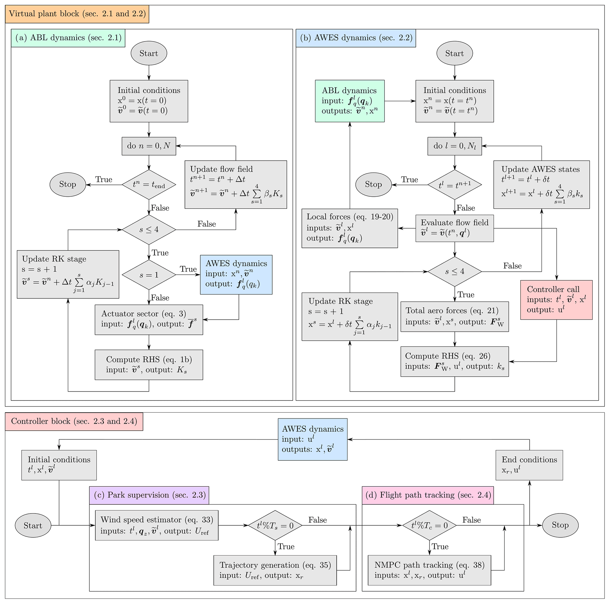
Figure 1Diagram representing the combined LES–OCP framework used in this study for the simulation of AWE parks in the ABL. Each part of the diagram refers to a specific feature of the framework. The diagram indicates the connections between the individual features and refers to specific subsections and the associated equations for a complete overview and discussion in the methodology section, Sect. 2.
The interaction between AWE systems and the atmospheric boundary layer requires a reciprocal coupling of both the system and flow dynamics. We have therefore developed a computational framework combining large-eddy simulations and optimal control techniques. The framework consists of two distinct blocks: the virtual plant, simulating the operation of AWE systems in a turbulent wind field, and the controller, supervising the plant performance and guaranteeing its operation. Figure 1 presents an overview of the different building blocks of the framework. The virtual plant is the executing organ of the framework and consists of two interconnected modules handling the coupled simulation of the ABL flow (Sect. 2.1) and AWES dynamics (Sect. 2.2) within the LES framework. The controller block is the deciding organ of the framework and is built on two hierarchical modules, the supervision level, which defines the reference trajectories flown by each AWE system in the plant (Sect. 2.3), and the tracking level, which computes the steering actions of each individual AWE system (Sect. 2.4).
2.1 Virtual plant: wind flow dynamics
The procedure applied to simulate wind flow dynamics is shown in Fig. 1a. The dynamics of the ABL are computed by means of large-eddy simulation (LES), and the effects of AWE systems on the flow are modelled using actuator methods. The LES methodology is presented in Sect. 2.1.1, and the actuator methods are introduced in Sect. 2.1.2.
2.1.1 Atmospheric boundary layer simulation
In the last decades, LES has become a widely used tool to model conventional wind farms in the atmospheric boundary layer (Calaf et al., 2010; Munters et al., 2016; Allaerts and Meyers, 2017), such that we adopt the same approach to investigate airborne wind energy parks. In LES methodology, large- and medium-scale flow structures are directly resolved with sufficient spatio-temporal resolution, whereas the influence of smaller-scale dissipative motion is modelled. The large, energy-containing structures, such as wind speed variations over regions spanning several hundreds of metres, play a predominant role in the energy extraction process of conventional and airborne wind energy systems alike. In LES computations, the transfer of energy across (a large part of) the inertial sub-range is further resolved, while the viscous dissipation of energy at the smallest scales is modelled using a subgrid-scale model.
In the current study, we neglect Coriolis and thermal effects, such that we only need to consider the turbulent surface layer of the ABL. In addition, the atmospheric flow through a wind farm is associated with a high Reynolds number such that we can omit the resolved effects of viscosity. Hence, the ABL can than be simplified to a pressure-driven boundary layer (PDBL) (Calaf et al., 2010). The PDBL is adequately modelled by the filtered incompressible Navier–Stokes equations for neutral flows, expressed by means of the continuity and momentum equations which are shown to read
The three-dimensional velocity field can be decomposed into its resolved component , for which we solve Eq. (1a) and (1b), and its residual component v′. The filtered velocity field is parameterised by its streamwise , spanwise , and vertical flow components. The continuity equation, Eq. (1a), enforces the solenoidal properties of the filtered velocity field. The momentum equation, Eq. (1b), contains the local acceleration of the flow on the left-hand side, while the right-hand side contains the convective acceleration and further collects the force contributions acting on the flow. The flow itself is driven by a constant imposed pressure gradient . The filtering operation results in a residual-stress tensor emulating the dissipation of kinetic energy at the sub-grid scales. The isotropic part of the residual-stress tensor is incorporated into the filtered modified pressure , while the deviatoric part of the residual-stress tensor τsgs is modelled using a closure model. Here, we opt for an eddy-viscosity Smagorinsky model with a height-dependent Smagorinsky length scale (Mason and Thomson, 1992), which reinforces the log-law behaviour of the ABL near the surface. Furthermore, an impermeable wall stress boundary condition is imposed at the bottom surface (Calaf et al., 2010). Finally, the body force term emulates the effects of AWE systems on the flow, for each of the Ns units of the park, by means of actuator methods, and its derivation is elaborated in Sect. 2.1.2.
Large-eddy simulations of AWE parks are performed with our in-house solver SP-Wind developed at KU Leuven. The governing equations are discretised using a Fourier pseudo-spectral method in the horizontal directions (x,y) and a fourth-order energy-conserving finite-difference scheme in the vertical direction z. These discretisation methods require periodic boundary conditions in the horizontal directions: we circumvent periodicity in the streamwise direction x by applying a fringe-region technique (Munters et al., 2016). This technique also allows one to provide unperturbed turbulent inflow conditions to the AWE park simulation by performing a concurrent-precursor periodic PDBL simulation in parallel to the main AWE park simulation. Time integration is performed using a classical four-stage fourth-order Runge–Kutta scheme.
2.1.2 Actuator methods
Actuator methods have proven their abilities to accurately reproduce wake characteristics of conventional wind turbines, such as the actuator line method (Sorensen and Shen, 2002; Troldborg et al., 2010; Martinez-Tossas et al., 2018) and the actuator sector method (ASM) (Storey et al., 2015). The dynamics of AWE systems and ABL flow span a large range of spatial and temporal scales: while the AWES wing experiences local wind speed fluctuations within a few metres along the wingspan, the ABL domain covers several kilometres. In addition, the flight dynamics of AWE systems are extremely fast and require a temporal resolution down to approximately 10 ms, whereas the large-scale flow structures evolve 1 to 2 orders of magnitude more slowly. Therefore, we opt for an actuator sector method that can both capture the local variations in aerodynamic quantities along the wingspans of individual AWE systems and accurately operate across a larger range of temporal scales. Similar to the actuator line method (ALM), the ASM projects the force distribution along the system wingspan onto the simulation grid of the LES, with an additional temporal smoothing that allows one to consider a larger time horizon than just one instantaneous position of the AWE system. The resulting projected force distribution hence depends on the main parameters of the LES, ie. the grid resolution of the flow domain, parameterised by the cell size Δx, Δy, Δz, and the simulation time step denoted by Δt, the time step of the AWE system dynamics denoted by δt, and a set of tuning parameters. While the methodology is outlined hereafter, Appendix A addresses the choice of LES settings and tuning parameters.
For the current AWE farm simulations presented later on, the cell size is Δx=10 m in the axial direction, and the LES time step is set to Δt=0.250 s. In order to achieve a stable simulation of AWE system dynamics, which are much faster and require a smaller time step, its value is set to δt=0.010 s. Accordingly, the kinematics of the AWE system (see Sect. 2.2.3) are evaluated 25 times per LES time step. The LES flow field is however only updated after each time step Δt; hence AWE systems operate, for the duration of an entire LES time step, in a frozen flow field evaluated at the beginning of the time step.
From the perspective of the AWE system, the time horizon between the instants tn and provides a static snapshot of the flow field and is further discretised into a collection of 25 sub-steps . At every sub-step tl, the local aerodynamic forces (per unit segment length) are computed along the aircraft wingspan given its instantaneous position ql in the frozen flow field. The procedure to compute is outlined in detail in Sect. 2.2.2. Subsequently, the local aerodynamic forces of each segment are smoothed out over the LES grid cells in the vicinity of the wing using a Gaussian convolution filter (Pope, 2000). The variance of the Gaussian distribution, where the width of the filter kernel is set to Δf=2Δx (Troldborg et al., 2010), is chosen to be similar to the second moment of the box filter. The instantaneous, spatially filtered forces, integrated over the complete normalised wingspan , read
When flying crosswind manoeuvres at high speed, the AWE system may fly through several LES cells within one simulation time step Δt. For conventional wind turbines, blade tips sweeping several mesh cells in one time step result in a discontinuous flow solution in the near wake (Storey et al., 2015). In order to avoid this discontinuity, the individual contributions of the spatially distributed forces can subsequently be weighted in time using an exponential filter (Vitsas and Meyers, 2016) given a certain time horizon, hence sweeping over a sector of the LES domain. The time-averaged force distribution is given by
The filter parameter γ is defined as with the filter constant τf=2ΔtLES. The force distribution is then added to the momentum equation, Eq. (1b). The size of the sector, i.e. the number of sub-steps sampled, depends on the stage of the Runge–Kutta time integration scheme. At the first stage, only the force distribution evaluated at tn is added to the previous sector. At the second and third stages, the force distributions between tn and are further considered. While for the fourth and last stage, the new sector consists of the entire range of sub-steps between tn and tn+1. Ultimately, the added force distribution accurately captures the fast and local dynamics of each individual AWE system and emulates their collective effects on the boundary layer flow.
2.2 Virtual plant: AWE system dynamics
The simulation strategy applied to AWE systems is shown in Fig. 1b. To describe and simulate the dynamics of AWE systems, there exist numerous models of varying complexity. These models range from fast quasi-steady models (Schelbergen and Schmehl, 2020) to simple 3DOF point-mass models (Zanon et al., 2013a) to complex 6DOF rigid-body models (Malz et al., 2019). The point-mass model allows the modelling of large-scale AWE systems while it does not require an extensive knowledge of the aircraft dimension and inertia, nor aerodynamic parameter identification, as is the case for the rigid-body model (Licitra et al., 2017). The point-mass model is therefore highly scalable. The model is also highly versatile and allows one to easily adapt generic wing designs to both ground-based and on-board generation AWE systems. In addition, the point-mass model has fewer states and control variables compared to the rigid-body model, resulting in a less computationally intensive model. Finally the point-mass model is tailored for the optimal control applications tackled in this work such as power-optimal trajectory generation and flight path tracking. Therefore, considering its simplicity and flexibility, we opt for the 3DOF point-mass model and present it in detail in Sect. 2.2.1.
Nevertheless, the 3DOF point-mass model also exhibits several limitations, mainly related to the lack of an explicit definition of the rotational dynamics of the system. Therefore, we derive the orientation and angular velocity of the system from state-based approximations. The approximations of orientation and angular velocity are further used to supplement the original point-mass model with a discrete lifting line model that takes into account local wind speed fluctuations for a more accurate representation of the AWE systems in the turbulent wind field. The procedure, which enables us to compute the instantaneous, local force distribution required in Eq. (2), is presented in Sect. 2.2.2.
Further, the equations of motion of AWE systems are derived from Lagrangian mechanics according to the procedure introduced by Gros and Diehl (2013) and outlined in Sect. 2.2.3.
2.2.1 Point-mass model
The architecture of AWE systems can be divided into three main key components: the ground station, the tether, and the airborne device. In this work, we assume that the ground station has no influence on the atmospheric flow and can therefore be neglected. In addition, we neglect tether dynamics such as tether sag and represent the tether as a rigid rod of varying length (Malz et al., 2019), which is solely subject to aerodynamic drag. At last, we limit our investigation to rigid-wing aircraft. Given the large level of approximation of the model, we simply assume that the wing planform is elliptical and without twist, which further allows us to simplify the aerodynamic properties of the finite wing (Anderson, 2010).
Hence, the tethered wing is modelled as a 3DOF point mass based on a representation of the system in non-minimal coordinates as proposed by Zanon et al. (2013b). The system state vector is composed of position q and velocity of the wing; the instantaneous aerodynamic quantities such as lift coefficient of the finite wing CL, roll angle Ψ, and on-board turbine thrust coefficient κ; and the tether variables l, , and , representing the length, speed, and acceleration of the tether respectively. In absence of explicit control surfaces such as ailerons, elevators, and rudders, we assume that the aerodynamic variables and the tether reel-out speed are directly and instantaneously controlled; hence we introduce the control vector , which consists of the time derivatives of lift coefficient, roll angle, and thrust coefficient and the tether jerk.
The 3DOF point-mass model only considers the translational motion of the AWE system, while the rotational motion is neglected. Hence, the aircraft attitude, commonly defined by the basis frame of the rigid body, is not known. Instead, we define the reference frame in which the external aerodynamic forces Fq acting on the system are expressed. First, we introduce the unit vector and the apparent wind speed va measured at the point mass. The apparent wind speed is defined as
where vw is the three-dimensional wind speed vector, computed from the neighbouring LES cells surrounding the point-mass position q using trilinear interpolation. Subsequently we define the basis vector , pointing along the apparent wind speed. Next, we introduce the perpendicular axis and the upward-pointing axis, which is orthogonal to the plane spanned by and reads . We apply a roll rotation of the perpendicular and normal axes about the axis ev≡eD by an angle corresponding to the state variable Ψ, which results in the transversal and lift axes
hence completing the basis of the frame of reference of the point mass . Furthermore, the basis vectors of Bpm are the columns of the rotation matrix .
Next, we can compute the aerodynamic forces acting on the point mass. These forces can be computed from the model states and the wind conditions, either solely measured at the point-mass position or along the complete wing span by using a more complex model, the lifting line model, introduced in the upcoming section, Sect. 2.2.2.
2.2.2 Lifting line model
The point-mass model provides the state and control variables that describe the flight path of the AWE system. The AWE system however operates in a turbulent boundary layer characterised by local fluctuations of the wind speed magnitude and direction, which, given the large-scale of the system's wing, considerably influence the force distribution along the wingspan. Therefore, we supplement the original 3DOF point-mass model with the lifting line model, which allows us to consider local fluctuations of (aero)dynamic quantities along the wingspan without adding complexity to the dynamics modelling and control of the aircraft. Hence, the wing is modelled as an aligned collection of discrete wing sections of width δs, for which we compute the aerodynamic forces based on the local wind condition.
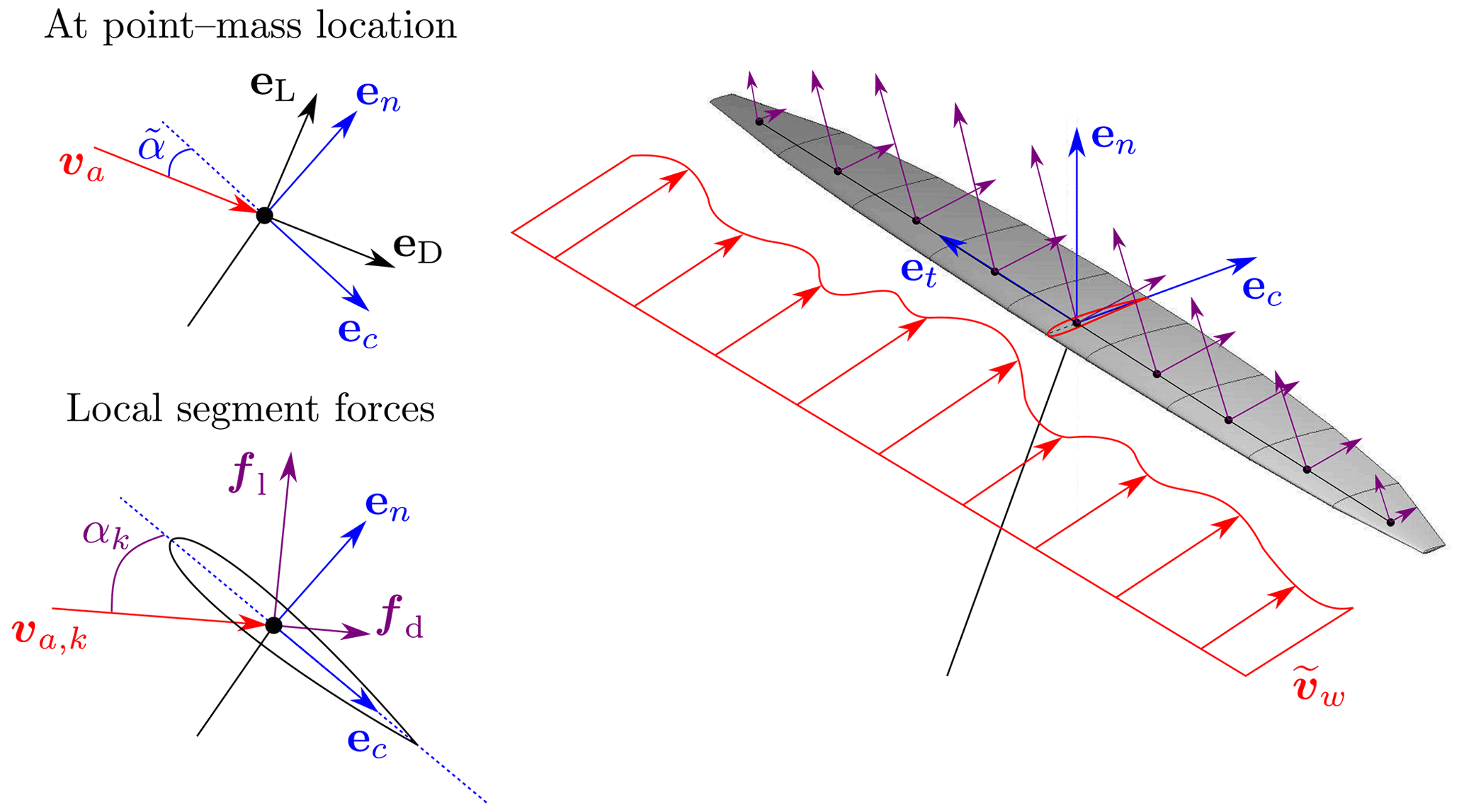
Figure 2Sketch of the configuration used in the lifting line model, showing the orientation of the AWE wing with respect to the incoming wind field and the aerodynamic forces fl and fd acting on the wing sections for a given apparent wind speed va,k.
The orientation of the wing is derived from a series of state-based assumptions building on the point-mass basis Bpm introduced above and resulting in a new orientation basis . Figure 2 shows a sketch of the wing configuration, and the derivations of the new orientation basis and of the local aerodynamic quantities are presented hereafter. First, we introduce the model-equivalent angle of attack , which we derive from the aerodynamic state CL and can be computed as for elliptical wings (Anderson, 2010). This model-equivalent angle of attack defines the a priori unknown orientation of the aircraft chord line . The transverse axis of the body-fixed frame et is aligned with the transverse axis of the point-mass frame eT, and the normal axis of the body-fixed frame is given as the cross product .
The rotation matrix R associated with the body-fixed basis B can be formulated in terms of Euler angles (Zanon, 2015) and can further be expressed as an extrinsic sequence of three consecutive rotations about the axes of the inertial frame
with the Euler angles , respectively representing yaw, pitch, and roll angles, and the associated rotations
The Euler angles are extracted from the entries rij of the orientation matrix R (Licitra et al., 2019):
The angular velocity ω of the aircraft can be derived from the Euler angle dynamics . Accordingly, we first approximate by a discrete backward difference,
and finally compute the angular velocity as
where, for the given sequence of rotations (Alemi Ardakani and Bridges, 2010), the mapping function inverse reads
The approximations of the angular velocity ω and the body-fixed basis frame R can then further be used to define the position and speed of discretised wing elements of the AWE system.
From the state-based approximations of attitude and angular velocity of the aircraft, we can now evaluate the position and speed of each wing section k, defined at the section centre, expressed in the inertial frame of reference as
where sk is the distance from the point mass to the segment centre given in the body-fixed frame. In this study, each AWES wing is discretised using 61 actuator segments. The spatial discretisation of the wing in the lifting line model allows us to account for the local fluctuations of the unsteady three-dimensional wind speed. The local wind speed vector vw,k is hence interpolated at the locations qk from the wind speed measured at the surrounding LES cells. We define the local apparent wind speed and compute the effective angle of attack αk seen by the airfoil of the wing section as
The local lift and drag coefficient cl(αk) and cd(αk) of each wing section are determined from aerodynamic polars obtained from 2D airfoil analysis mentioned in Sect. 3.1.
The air density at each wing section is computed from the standard atmosphere density model (Archer, 2013) and reads
where p0=1013.25 hPa and T0=288.15 K are the reference pressure and temperature measured at sea level, g=9.81 m s−2 is the gravity constant, K m−1 is the average lapse rate in the atmosphere, and R=287.058 J kg−1 K−1 is the specific gas constant of dry air.
The chord length of each wing section is computed from the elliptical planform distribution of the wing according to
where b is the wingspan and AR the aspect ratio of the AWES wing. The values of b and AR are further discussed in Sect. 3.1. Finally, we can compute the local aerodynamic forces per unit segment length acting on each segment section. The instantaneous contributions of aerodynamic lift and drag forces read
Similarly, for drag-mode AWE systems, the additional drag of on-board turbines is distributed over ng actuator segments, covering the central third of the wingspan. We assume that the individual on-board turbines all operate at the same value of the generator thrust coefficient κ, such that the local generator drag reads
for specific segments or is zero otherwise. The instantaneous local section force per unit segment length at the time instant tl contains the sum of local lift forces, drag forces, and, if applicable, on-board turbine forces. This total force reads and can further be broadcast to Eq. (2) to be later added to the LES flow equations, Eq. (1b), or integrated over the complete wingspan to define the instantaneous total aerodynamic forces acting on the wing :
2.2.3 AWE system dynamics
In the current procedure, the system configuration is described by its set of generalised coordinates q, and its motion is restricted by the constraint c(q)=0, with which we associate the Lagrange multiplier λ. For the tethered single-wing AWE system configuration considered in this study, the point mass is constrained to the manifold described by
In order to obtain an index-1 differential algebraic equation (DAE) that can be integrated with Newton-based numerical methods, an index reduction is performed by differentiating the constraint (Eq. 22) twice (Gros and Diehl, 2013). Baumgarte stabilisation combined with periodicity constraints in the optimal control problem then ensures that the consistency conditions c(q)=0 and , are satisfied during the entire power cycle (Gros and Zanon, 2018). The motion of the AWE systems is then defined by the set of equations
In Eq. (23a), and define the effective inertial mass and the effective gravitational mass (Houska and Diehl, 2007), with mW and mT representing the mass of wing and tether and Fq the aerodynamic forces acting on the system. In Eq. (23b), p=10 is a tuning parameter of the Baumgarte stabilisation scheme.
The total aerodynamic force acting on the system Fq consists of the sum of wing forces FW from Eq. (21) and tether drag forces FT. The total tether drag (Argatov and Silvennoinen, 2013) is given by
with the tether diameter dT and the drag coefficient of a cylinder Ccyl=1.0 at high Reynolds numbers.
The acceleration and control inputs u are obtained by respectively solving the DAE system (Eq. 23) and the path tracking problem (Eq. 36) detailed in Sect. 2.4. Finally, the kinematics of the AWE systems read
The kinematics of the systems (Eq. 25) are further integrated in time using an internal four-stage fourth-order Runge–Kutta scheme with a sub-step size δt as previously mentioned in Sect. 2.1.2.
Unfortunately, directly feeding the lifting line forces FW (Eq. 21) into the AWE system dynamics (Eq. 23) in combination with the non-linear model predictive control (NMPC), presented later in Sect. 2.4, is not possible: the mismatch between the aerodynamic forces generated by the lifting line and the aerodynamic model of the point-mass assumed by the controller does not lead to a stable system in our implementation. Therefore, in order to reduce the model mismatch between plant and controller, we compute the total wing force at the point-mass position using the aerodynamic states as , where the individual contributions of wing lift, wing drag, and on-board turbine drag are given by
This approach, while it still takes into account the unsteadiness of the LES wind field when computing the apparent wind speed va at the point-mass location from Eq. (4), results in a satisfactory tracking performance of the controller.
2.3 Controller: park supervision
The procedure defining the supervision level of the AWE park is shown in Fig. 1c. The supervision level contains two modules: the wind speed estimator, presented in Sect. 2.3.1, and optimal trajectory generator, presented in Sect. 2.3.2. For each AWE system, the wind speed estimator samples the local wind conditions monitored at the wing and derives an approximation of the associated vertical wind profile. These wind profiles are further communicated to the trajectory generator and used to generate periodic power-optimal reference trajectories flown by each system individually.
2.3.1 Wind speed estimator
The controller does not have knowledge of the unsteady three-dimensional wind field from the LES and hence assumes that the wind field is given by a one-dimensional, height-dependent profile , where the streamwise wind speed component U(qz) is given by the logarithmic distribution
The logarithmic distribution is parameterised by a reference speed Uref given at an altitude zref and by a surface roughness length z0. Further, we consider offshore conditions such that the surface roughness height is z0=0.0002 m (Troen and Lundtang Petersen, 1989), and we will use the altitude zref=100.0 m as reference height at which the reference wind speed Uref is measured.
When extracting power from the wind, conventional and airborne wind energy systems alike exert a thrust force on the incoming flow field (Jenkins et al., 2001). This process results not only in a velocity decrease downstream of the system, the wake, but also in a velocity decrease upstream of the system, the induction region. Upstream flow induction reduces the available power that wind energy systems can harvest. From one-dimensional momentum theory, it was shown for conventional wind turbines modelled as actuator discs that the velocity decrease across the actuator can be defined as
where the unperturbed inflow wind speed is denoted as U∞, while UD and UW respectively represent the wind speed at the actuator disc and in the wake. The axial induction factor a quantifies the strength of the induction phenomenon. The values of axial induction factors reported in AWE literature (Leuthold et al., 2017; Haas and Meyers, 2017; Kheiri et al., 2018) are lower than the known Betz limit of conventional wind turbines (Jenkins et al., 2001), suggesting that axial induction is less significant for airborne wind energy systems, although it cannot be fully neglected. In the current approach, the LES-based wind velocity sampled by the wind speed estimator already contains the effects of axial induction. Hence, optimal trajectories are later generated for reference wind speeds Uref, computed by the wind speed estimator, and equivalent to the actuator-based wind speed UD instead of the inflow wind speed U∞.
For each AWE system, the wind speed estimator monitors the system altitude and LES-based wind velocity measured at the point mass. In practice, the value of the wind speed can be derived from the measured airspeed using on-board instrumentation. From the monitored time series, we approximate the vertical wind speed profile by estimating the related reference wind speed Uref by means of a running-time average. For lift-mode AWE systems, the wind speed and altitude are sampled during one full periodic cycle consisting of four power generation loops and one retraction phase. For drag-mode AWE systems, the data series are collected during five single-loop power cycles. The range of flight altitude z≡qz collected during the sample period Ts defines the sample space variable with . Over the interval H, the mean wind speed measured at the point mass for the duration of the sampling period Ts is given by
The mean wind speed, integrated from the logarithmic profile over the same interval h, is a linear function of the actuator speed and is given by
Hence we can derive the reference value of the logarithmic wind profile that best approximates the wind conditions monitored by each AWE system during the sample period Ts as
We further use this value to generate the associated reference trajectories as we show in Sect. 2.3.2.
2.3.2 Generation of reference trajectories
In this study we generate a set of reference flight trajectories by using optimal control techniques. Optimal control techniques allow us to optimise the flight of the AWE system for different objectives while respecting a large number of constraints during operation. First, we can generate power-optimal reference trajectories optimised for various flow conditions, as shown hereafter. Second, optimal control also allow us to perform path tracking of the reference trajectories in the turbulent LES flow field, as shown in Sect. 2.4.
The Lagrangian modelling procedure applied to a tethered point mass proposed in Sect. 2.2.1 results in an implicit index-1 DAE given by Eqs. (23) and (25). This representation can be summarised by
In addition to the state and control vectors x and u, and the algebraic variables z=(λ) previously defined, we introduce an additional optimisation parameter θ and a set of constant parameters p, which allow us to apply the optimisation problem for a number of AWE designs and wind conditions. The optimisation parameter θ=dT is the tether diameter and is optimised to sustain maximal tension TT,max during operation. The set of constant parameters contains the dimensions of the aircraft – its wing mass mW, wingspan b, and aspect ratio AR, and the wind conditions are parameterised by the reference wind speed and altitude ,Uref and zref, and the roughness length, z0.
During operation, the AWE systems have to satisfy a set of constraints that ensure a hardware-friendly operation and the manoeuvrability of the aircraft. Hence, for the dynamics (Eq. 32) and constraints h, we can formulate a periodic optimal control problem (POCP) with a free time period Tp as
The cost function is defined as the average mechanical power output of the system generated over a full cycle of period Tp. The instantaneous power generated by lift- and drag-mode AWE systems respectively reads
For lift-mode AWE systems, power is generated by unwinding the tether from the winch at a speed under the high tether tension TT=λl generated by the aerodynamic forces acting on the wing. The power generation phase consists of four loops and is followed by the retraction phase to wind the tether back up on the winch. For drag-mode AWE systems, power is extracted from the wind by on-board generators. These generators are modelled as actuator discs such that the power is equivalent to the turbine thrust force multiplied by the wind speed measured at the disc . Here, ηr=0.8 is the rotor efficiency and characterises the ability of the on-board turbines to extract power from the surrounding flow, ie. the axial induction associated with the actuator disc assumption. In line with Echeverri et al. (2020), where ηr is defined as rotor efficiency from thrust power to shaft power, Eq. (35) defines the mechanical power that drag-mode AWE systems can extract from the wind.
The trajectory and performance of AWE systems depend on the path constraints and variable bounds specified in the periodic optimal control problem (Eq. 33c). Tables 1 and 2 summarise the chosen constraints and bounds specified for trajectory optimisation. The path constraints and variable bounds used in this work are compiled from the available literature (Gros and Diehl, 2013; Licitra et al., 2016; Zanon et al., 2013b; Kruijff and Ruiterkamp, 2018) and are adapted to large-scale AWE systems. These choices are motivated hereafter. We set an operational upper limit to the tether length lmax=1000 m. We also limit the operation range of the winch by setting bounds to the tether speed and acceleration . In addition, the aerodynamic lift coefficient of the wing CL is restricted to the range [0.0, CL,opt], where . The lower bound ensures that the tether tension remains positive at all times while the upper bound limits local stall along the wing. The value of the upper bound CL,opt stems from Fig. 5, and its choice is further discussed in Sect. 3.1. The roll angle Ψ is bounded in order to ensure safe operation, i.e. avoid collision between the tether and the airframe, and also take into account the reduced manoeuvrability of the large-scale aircraft. Next, the maximal tether tension and the maximal acceleration are limited to ensure the integrity of the aircraft. The former also ensures that maximum tether stress is not exceeded by considering a safety factor fs=3 and a tether yield strength σmax=3.09 GPa. Further, we constrain the operation range of the control variables in order to avoid aggressive pitch and yaw manoeuvres, which are not suited to large-scale aircraft. The bounds on u are derived using a heuristic approach in order to avoid unrealistic values of the approximated angular velocity. The spatial footprint of the trajectories is limited by means of spatial constraints, limiting the axial, lateral, and vertical extents of the trajectories in order to achieve system packing densities of , as later discussed in Sect. 3.3.
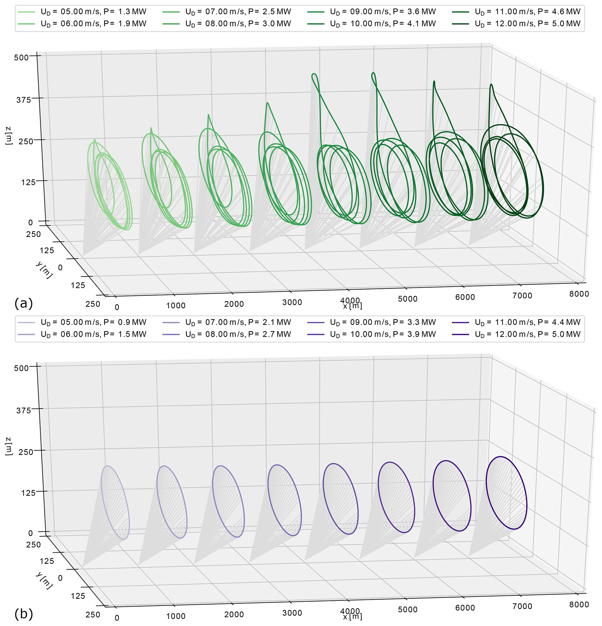
Figure 3Power-optimal trajectories of (a) lift- and (b) drag-mode AWE systems optimised for the range of wind speed by solving the optimal control problem (Eq. 33) under consideration of the variable constraints given in Tables 1 and 2. The maximal streamwise extent of each trajectory does not exceed 1000 m, but for the sake of visualisation the positions of successive ground stations were shifted by 1000 m.
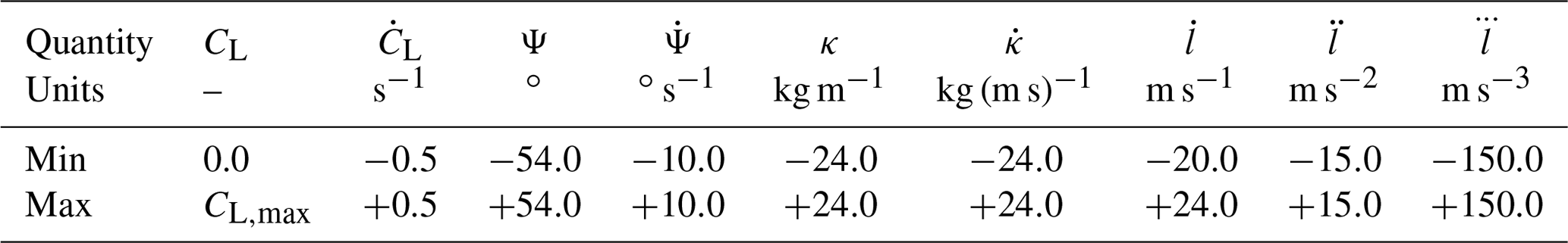
Table 1Bound constraints applied to state variables x used in the optimal control problem (Eq. 33). The maximal lateral extent of the flight path and the maximal tether length are respectively set to ymax=250 m and lmax=1000 m to limit the footprint of the trajectories. The optimal value of the lift coefficient is .
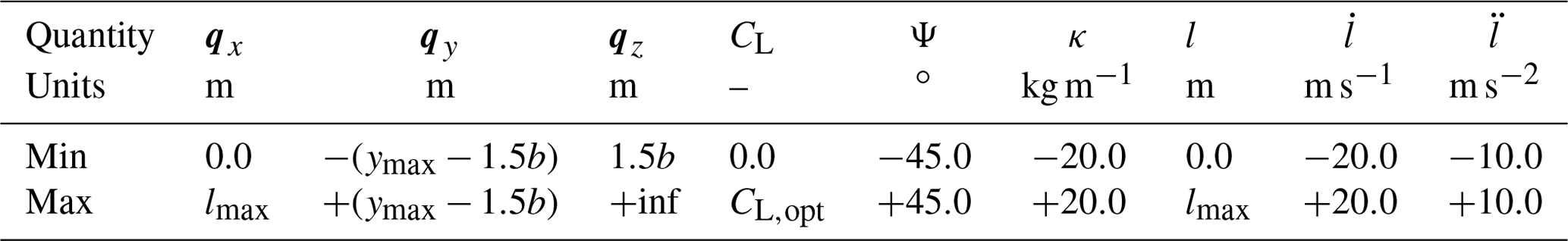
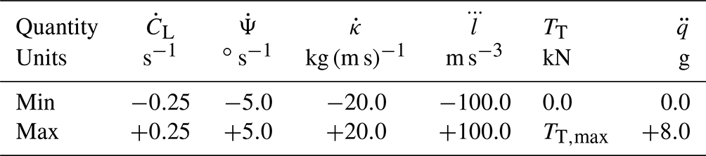
Table 2Bound constraints applied to control variables u and other variables used in the optimal control problem (Eq. 33). The maximal tether tension depends on the wing design and is discussed in Sect. 3.
In practice, the reference trajectories are optimised off-line for a specific range of wind speeds. We aim to operate the AWE systems below the rated wind speed, in the so-called region II (Leuthold et al., 2018), where the harvested power increases with the wind speed. Hence we generate a library of optimal trajectories (OTL) for a range of actuator-based wind speeds with an increment ΔUD=0.25 m s−1. Figure 3 shows the different trajectories computed for the range of wind speeds. At the end of the sampling period Ts, the controller verifies whether the reference wind speed from Eq. (31) has changed, and if so, chooses the closest value in the range [5.0, 12.0] and commands the AWE system to track the new trajectory defined by the reference states xr. The wind speed dependency of the trajectories is presented in Appendix B, Figs. B1 to B4.
2.4 Controller: flight path tracking
The procedure defining flight path tracking is shown in Fig. 1d. In the LES-generated virtual wind environment, the operation conditions of the AWE systems differ substantially from the model assumptions in Eq. (27). The complex dynamics make the motion of the AWE system highly sensitive to fluctuations. Therefore a control algorithm is required to lead the system onto its pre-computed optimised reference trajectory. Accordingly we apply non-linear model predictive control (NMPC) (Gros et al., 2013). For a moving time horizon, the NMPC repeatedly computes the optimal control inputs that reduce the error between the current states x and the states xr of the reference flight path taken from the OTL. Therefore, we can formulate for the prediction horizon Tc a new optimal control problem (Eq. 36).
The cost function (Eq. 36a) is formulated as a least-square objective, defining the tracking error between the current states x(t) and the given reference xr(t), with a penalisation on the deviation from both the reference states and controls. Just like for the generation of periodic optimal trajectories, the constraints (Eqs. 36b and 36c) enforce the system dynamics and path constraints, while the initial condition (Eq. 36d) ensures that the initial states match the current estimate . An additional terminal condition (Eq. 36e) ensures the system finds the reference at the end of the prediction horizon. Some of the path constraints in Eq. (36c), in particular the aerodynamic states and the control variables, are relaxed compared to the POCP bounds in Tables 1 and 2. This allows the controller to handle wind disturbances and plant–controller model mismatch with a wider range of steering strategies. Table 3 summarises the NMPC constraints and bounds adapted for trajectory tracking. The maximal allowed lift coefficient corresponds to the upper bound of the validity range of the linear lift slope of the elliptical wing. Similarly to CL,opt for the trajectory generation, the value of the upper bound CL,max stems from Fig. 5, and its choice is discussed in Sect. 3.1. In addition, the maximal allowed tether tension and acceleration are relaxed by respectively 10 % and 20 %.
Table 3Relaxed variable bounds used in non-linear model predictive control (Eq. 36). The maximal value of the lift coefficient is .
To solve the optimal control problems, we use the awebox toolbox (awebox, 2021). In the toolbox, both trajectory generation and flight path tracking OCPs are discretised using the direct collocation approach based on a Radau scheme with a fourth-order polynomial. The resulting nonlinear program is formulated using the symbolic framework CasADi (Andersson et al., 2018) and solved with the interior-point solver IPOPT (Wächter, 2002) using the linear solver MA57 (HSL, 2011). More information about the implementation can be found in De Schutter et al. (2019).
The different AWES park configurations investigated in the current work are presented hereafter. First, we detail the design choices behind the large-scale lift- and drag-mode AWE systems in Sect. 3.1. Next we discuss the mode-specific operation of both the lift- and drag-mode AWE systems, in particular the effects of wind speed on the system performance, in Sect. 3.2. Finally, we specify the computational settings of the performed LES of the atmospheric boundary layer and present the different AWES park layouts used in this study in Sect. 3.3.
3.1 Design of large-scale AWES
For given wind conditions and space constraints, wind farm developers design their parks so as to optimise several design metrics. Traditionally, these metrics include the annual energy production (AEP) and the levelised cost of energy (LCOE) (Dykes, 2020). In order to minimise the LCOE, wind farms of conventional wind turbines in the range 10–15 MW target power densities of approximately 5 MW km−2 (Bulder et al., 2018). For the large-scale deployment of their technologies, AWE manufacturers have engaged in the development of utility-scale multi-megawatt AWE systems for offshore operation generating up to 5 MW of power (Kruijff and Ruiterkamp, 2018; Makani Power, 2012). Also, the AWE manufacturer Ampyx Power aims at achieving farm level power densities in the range of 10–25 MW km−2 with their commercial systems (Kruijff and Ruiterkamp, 2018). Accordingly, when designing parks of AWE systems, one has to define first the type of AWE systems used to harvest power and second the layout of the farm that will ensure a safe operation while maximising the power density.

Figure 4Aerodynamic polars of the SD 7032 airfoil generated at a chord-based Reynolds number Rec=107 with XFLR5: (a) lift coefficient polar and (b) drag coefficient polar. The dashed lines show the coefficient values past the critical angle of attack αc≈17.7∘. The zero-lift angle of attack of the airfoil is ∘ while the profile drag coefficient is .
Hence, we propose a generic design for lift- and drag-mode AWE systems that is easily scalable and allows one to model the operation of AWE systems in various wind conditions. The wingspan b of the wing is chosen as the driving design parameter to describe the dimensions of the different systems while the wing aspect ratio is fixed to AR=12, similar to the AWE systems developed by Ampyx Power. Design considerations such as manufacturability or structural analysis of the wing lie outside of the scope of the study. Therefore, a wing with elliptical planform is chosen here for simplicity. Elliptical wings exhibit advantageous aerodynamic properties given that their planforms generate low induced drag. Nevertheless, their stall characteristics are unfavourable: elliptical wings generate a constant downwash along the wingspan. Therefore, in the absence of geometric twist and for a uniform airfoil distribution, the induced angle of attack is constant along the wingspan. As a consequence, the effective angle of attack of each wing section is equal, which might cause the entire wing to stall simultaneously. Elliptical wings provide an analytical formulation of the aerodynamic lift and drag coefficients of the wing (Anderson, 2010):
where αg is the geometric angle of attack of the wing. In addition, αL=0 and Cd,0 respectively represent the zero-lift angle of attack and profile drag coefficient of the airfoil. The lift slope a of the finite wing is given by , with a0=2π the airfoil lift slope from inviscid flow theory. The discussed properties of the elliptical wing and the aerodynamic coefficients given in Eq. (37) are valid for steady-state level flight; nevertheless they will be used as a surrogate model for the wing of the AWE system: this model is used to approximate the wing orientation in the lifting line model introduced in Sect. 2.2.2 and to derive the state bounds of CL in the AWES model of the controller in Sect. 2.3 and 2.4. Unsteady aerodynamic effects, which are not considered here but might play a significant role for AWE systems, need to be addressed in the future.
In order to achieve a high lift-to-drag ratio, we opt for airfoil sections of type SD 7032, also used by the manufacturer TwingTec (Gohl and Luchsinger, 2013). The lift and drag polars of the airfoil are computed from an XFOIL direct analysis using the open-source software XFLR5 (XFLR5, 2021) at a chord-based Reynolds number Rec=107 and shown in Fig. 4. From the airfoil analysis, we can retrieve the values of the zero-lift angle of attack ∘, of the critical angle of attack αc=17.7∘, and of profile drag coefficient . Past the critical angle of attack αc, the airfoil is subject to stall, characterised by a drop of the lift coefficient and a sharp increase in the drag coefficient.
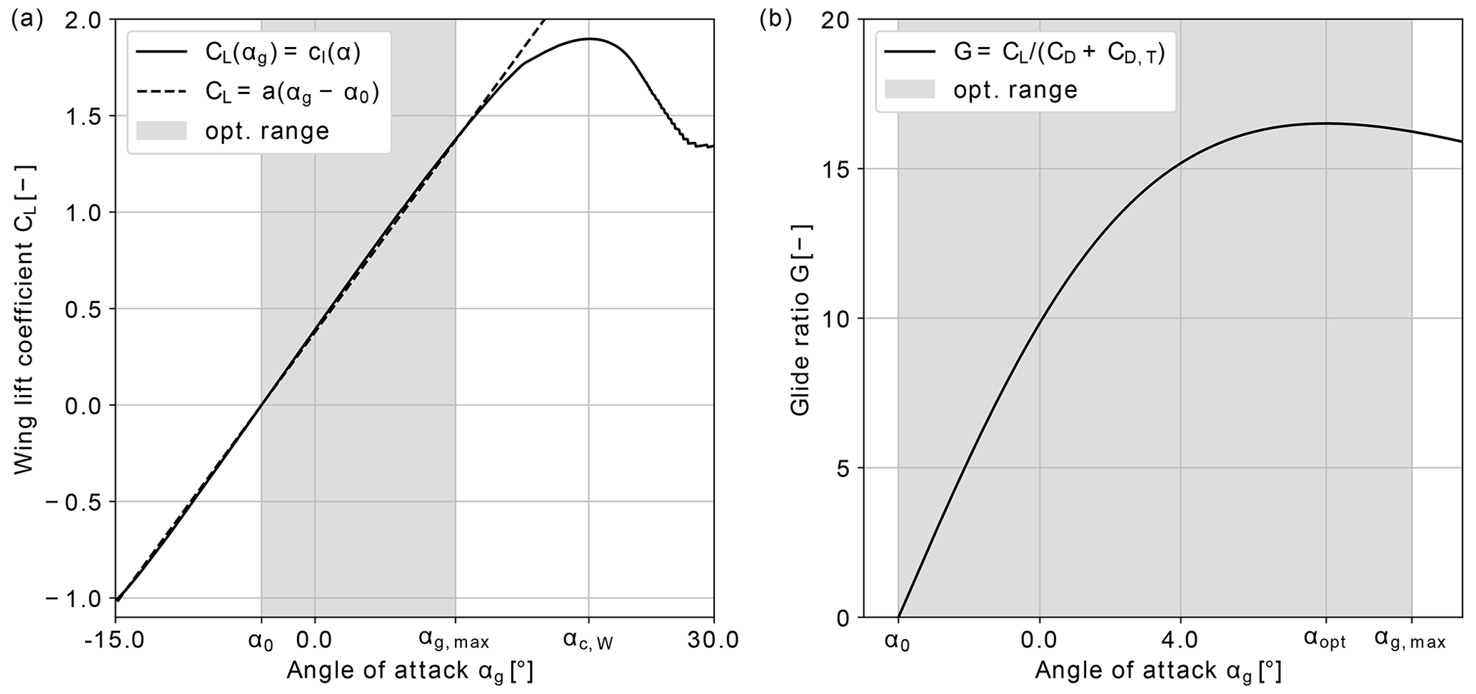
Figure 5Aerodynamic quantities of the finite wing with aspect ratio AR=12: (a) wing lift coefficient and (b) glide ratio. The shaded area shows the optimisation range of the optimal control problems (Eqs. 33 and 36) in between the zero-lift angle of attack of the airfoil ∘ and the maximal value αmax≈10.6∘ of the validity range of linear approximation (Eq. 37). The critical angle of attack of the wing is ∘, and the angle of attack corresponding to the maximal value of the glide ratio is αopt≈8.1∘.
The lift and drag predictions of XFOIL are only valid just beyond αc (XFOIL, 2021). In addition, the distribution of angles of attack in the lifting line model can vary substantially along the wingspan, due to the spatial fluctuations of the LES-based wind velocity and the speed difference between the two tips of the aircraft. Therefore, the operation of the AWE system is to be optimised such that not only the adverse effects of stall are avoided but also an accurate prediction of the aerodynamic behaviour of local wing sections of the lifting line is ensured. To do so, we restrict the values of the state variable CL, and equivalently the values of the model-equivalent angle of attack , to a range well below stall, as explained hereafter.
The linear approximation of the wing lift coefficient given in Eq. (37) is only valid for the range of angles of attack up to ∘, well below the critical angle of attack of the wing ∘, as shown in Fig. 5a. Therefore, the upper bound of CL is set to a value that maximises the glide ratio G of the tethered wing system: the glide ratio is defined as the ratio of aerodynamic lift forces to the combined contribution of wing and tether to the overall drag forces (Diehl, 2013). The contribution of the tether is given as with the drag coefficient of a cylinder at high Reynolds number Ccyl=1.0. For the targeted wingspan of 60 m and an expected tether diameter of m, the maximal glide ratio G≈16.5 is achieved at a geometric angle of attack of αg≈8.1∘ and results in , as shown in Fig. 5b. Consequently, the upper bound of the wing lift coefficient is in the POCP (Eq. 33) and in the NMPC (Eq. 36). A discussion of the angle of attack and load distributions of the trajectories optimised with Eq. (33) and using this approach is presented in Appendix A2.
The remaining necessary dimensions of the AWE systems are derived from a semi-empirical study based on available manufacturer data, where we derive the wing mass and tension limits from the wingspan b. We set an upper bound to the tether tension and assume that it scales linearly with the surface area of the wing. Further we assume that the targeted AWE system with a 60 m wing with aspect ratio 12 can sustain up to approximately 850 kN of pulling force from the tether. Further, the wing mass is estimated by fitting a power law onto data from the manufacturer Makani Power taken from Makani Power (2012) as shown in Fig. 6. Hence wingspan-based relations for the maximal tether tension and the wing mass read
with the parameters γ1≈2840.24, γ2≈0.1478, and γ3≈2.662. Note that for lift-mode AWE systems, the wing mass is reduced by 25 % in order to account for the absence of on-board turbines. Finally, the tether material is assumed to be Dyneema for both types of AWE systems. This material is commonly used by AWE manufacturers and has a density ρT=970.0 kg m−3.
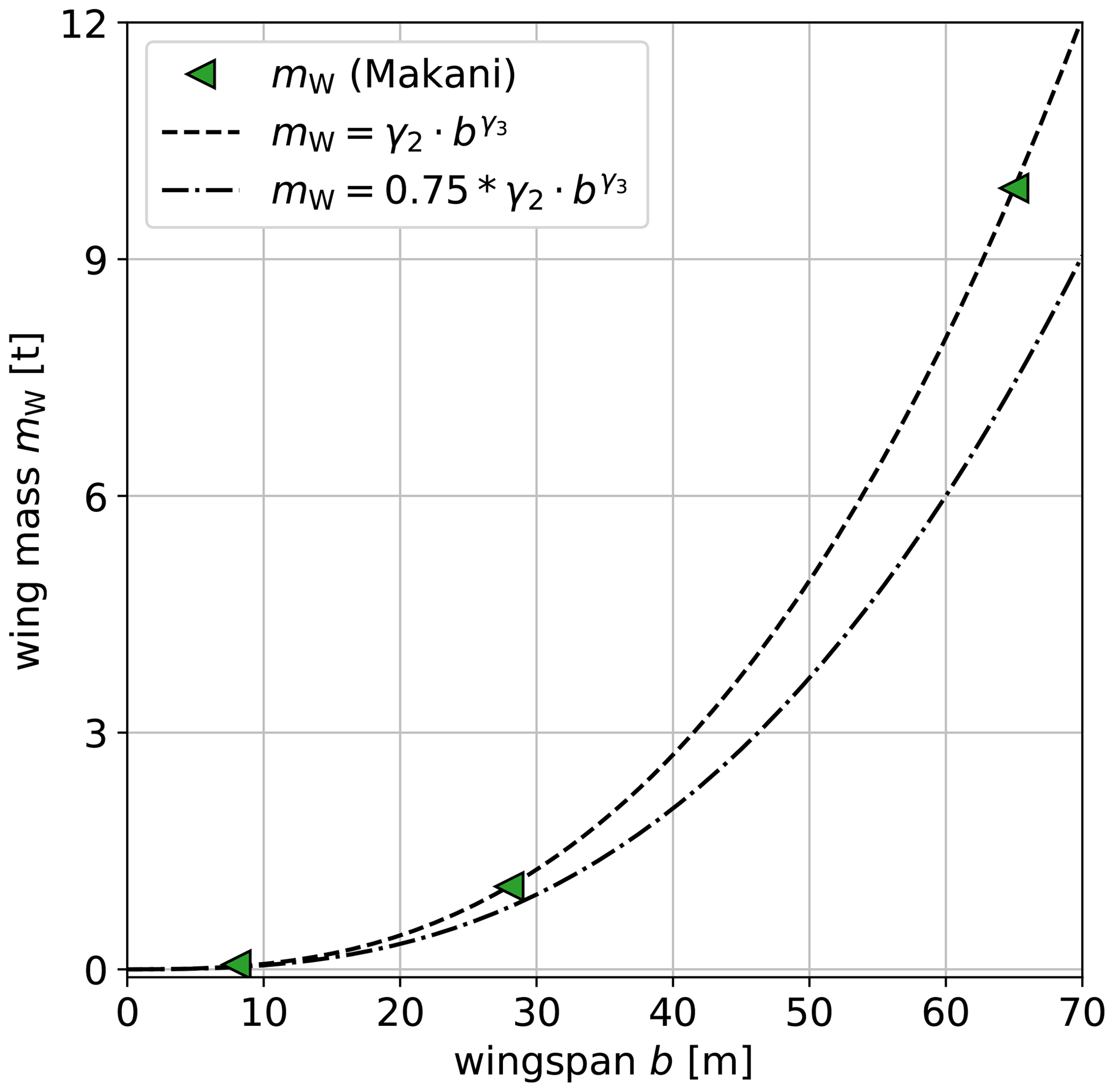
Figure 6Scaling of the wing mass with the wingspan of the aircraft based on manufacturer data from Makani Power (Makani Power, 2012). The dashed line shows the power law fitted from data with γ2≈0.1478 and γ3≈2.662 used for drag-mode AWE systems while the dashed–dotted line shows the power law with a 25 % reduction of the mass as used for lift-mode AWE systems.
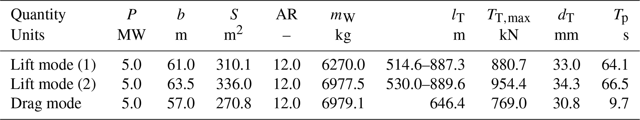
Table 4Wing and tether characteristics of the reference trajectories optimised for lift- and drag-mode AWE systems at rated wind speed UD=12 m s−1 under consideration of offshore conditions.
3.2 Operation of large-scale AWE systems
We apply the optimisation procedure outlined in Sect. 2.3.2 to optimise the dimensions and flight path of three different AWE systems targeted at offshore operation and capable of generating 5 MW of rated power for a design wind speed UD=12.0 m s−1. We design and optimise one drag-mode AWE system and two different lift-mode AWE systems, of which we discuss the operation characteristics in Sect. 3.2.1. Table 4 summarises the main dimensions of wing and tether of the three considered AWE systems. For lift-mode AWE systems, preliminary work on single AWE systems has highlighted the effect of reel-out speed on the instantaneous flow conditions experienced by the system. Therefore, we use two different reel-out strategies for the operation of lift-mode AWE systems, which we discuss in Sect. 3.2.2. The details of the single AWE system analysis are given in Appendix A. The first strategy uses the hypothetical physical limitations of the winch, where we assume that the maximal reel-out speed is m s−1 as given in Table 1. However, given that the optimisation procedure does not take the generation of the system wake into account, the wing can potentially interact locally with its own wake during the reel-out phase as discussed in Sect. 3.2.2. Therefore, the second strategy limits the maximal reel-out speed to the expected advection speed of the wake UW as estimated in Eq. (28a) and (28b). While the value of the induction factor a is a priori unknown, we opt for the conservative guess a=0.25 based on an empirical choice, such that the maximal reel-out speed of the tether becomes wind-speed-dependent and is shown to read
Given that the individual AWE systems in the farm operate in different wind conditions, we also generate their trajectories for a large range of wind speeds below rated wind speed. Hence, each system can adapt its flight path and power performance to the temporarily experienced wind field as introduced in Sect. 2.3. The effects of varying wind speed on the AWE system trajectories are discussed in Sect. 3.2.3.
3.2.1 Operation at rated wind speed
At rated wind speed, the drag-mode AWE system and the two lift-mode AWE systems all generate 5 MW of power. However, their flight path and power generation profile differ substantially as shown in Fig. 7. A complete description of all system states, controls, and additional metrics is given in Appendix B, and their main features are summarised here.
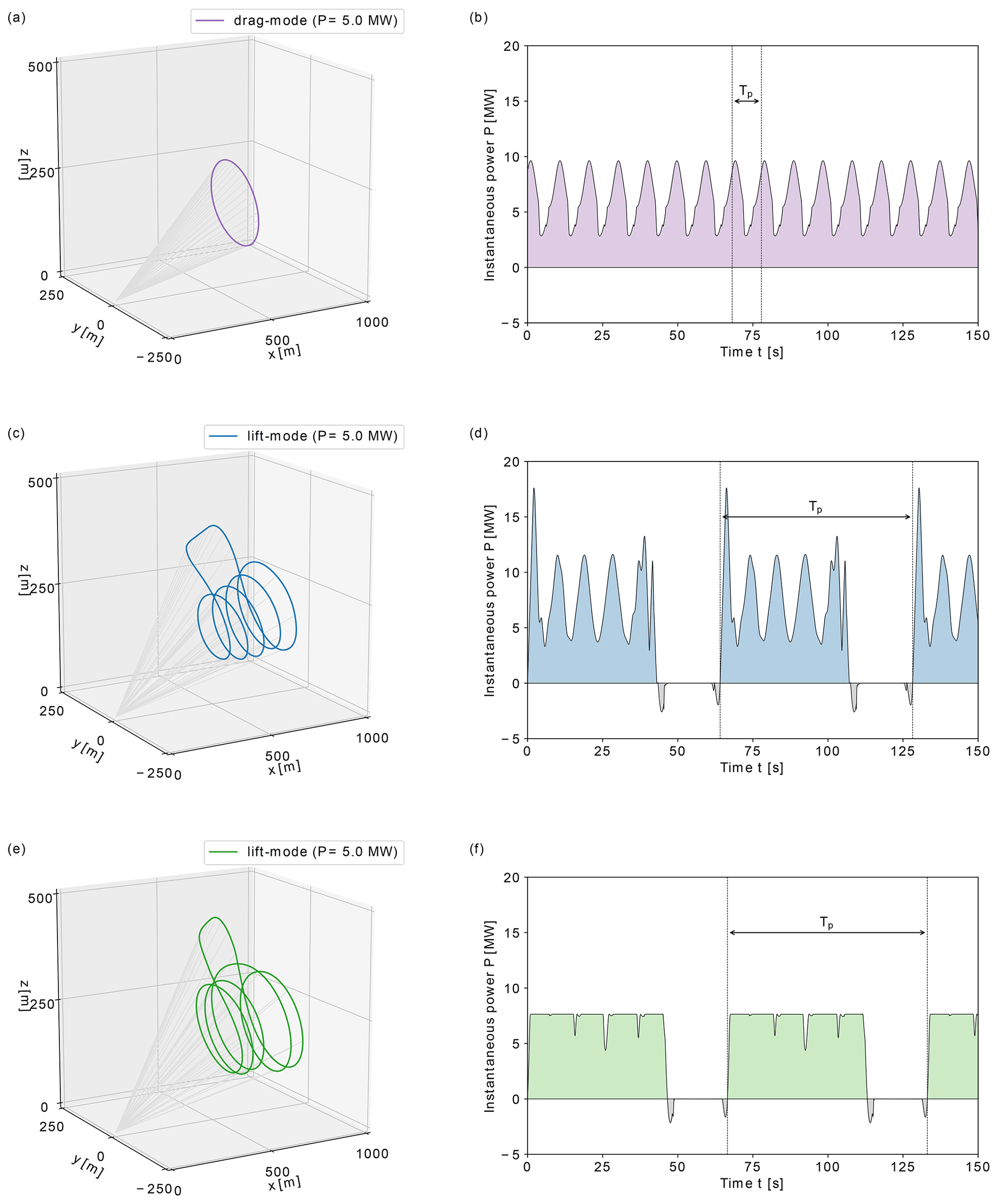
Figure 7Flight path and instantaneous power of 5 MW reference lift- and drag-mode AWE systems optimised for given rated wind speed UD=12 m s−1 under consideration of offshore conditions. (a, b) Drag-mode AWE system, (c, d) lift-mode AWE system (1) with original bounds, and (e, f) lift-mode AWE system (2) with induction-based limitation of reel-out speed.
The drag-mode AWE system operates at a constant tether length l≈650 m and follows a near-circular flight path of diameter D≈200 m at a mean elevation of about 17∘. The duration of a single-loop periodic cycle equals approximately 10 s. The system operates at maximal tether tension, maintaining a high flight speed between 60 and 80 m s−1 throughout the cycle. The on-board turbines of the system continuously generate power while reaching peak generation during the downward flight when the maximal flight speed is achieved.
For the two lift-mode AWE systems, one periodic cycle consists of four power-generating loops and a retraction phase. The duration of the periodic cycle ranges between approximately 64 and 66 s, while the reel-out phase accounts for about 70 % of the cycle. During the reel-out phase, the tether length varies approximately between 500 and 900 m, while the loop diameter ranges between 200 and 250 m and the mean elevation angle is approximately 19∘. Mechanical power is generated by reeling out the tether at high speed under maximal tether tension. The retraction phase consists of a steep upward flight at maximal tether length to transition out of the last power generation loop, followed by the reel-in phase of the tether at high altitude, and is completed by a dive manoeuvre to transition into to the new power generation phase. During the retraction phase, the tension on the tether is minimal, and a fraction of the generated power is used to reel in the tether. With the first reel-out strategy, the reel-out speed fluctuates during each individual loop, reaching its peak during the downward flight, resulting in large variations in instantaneous power generation. The flight speed of the systems remains nearly constant during the duration of the production phase, fluctuating between approximately 60 and 70 m s−1. With the second strategy, the reel-out speed of the tether is capped by the induction-based constraint such that the tether is reeled out at a nearly constant speed. Accordingly, the generated power remains nearly constant during the generation phase. Given the reel-out speed limitation, part of the kinetic energy of the system is used to accelerate the system during the downward flight, resulting in large fluctuations of the flight speed in the range 60 to 90 m s−1.

Figure 8Instantaneous lateral snapshots of the wake field of reference lift-mode AWE systems operating in an unperturbed logarithmic inflow at a wind speed UD=10 m s−1. Isovolumes of positive Q criterion, coloured by streamwise velocity for (a) lift-mode AWE system with original bounds at t=301 s and (b) lift-mode AWE system with induction-based limitation of reel-out speed at t=313 s.
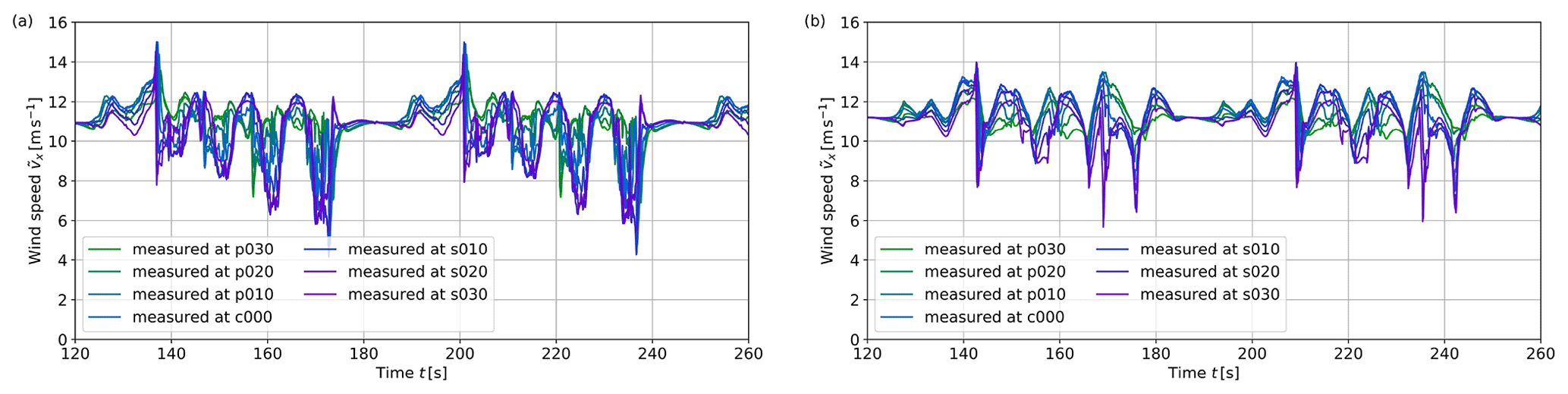
Figure 9Instantaneous values of streamwise velocity measured at several locations along the wingspan for (a) lift-mode AWE system with original bounds and (b) lift-mode AWE system with induction-based limitation of reel-out speed. The prefixes “p” and “s” stand for the port and starboard sides of the wing, while the prefix “c” stands for the centre, i.e. the point mass. Furthermore, the numbers stand for the segment positions on each side of the wing, from 0 at the centre to 30 at the wing tip.
3.2.2 Characteristics of lift-mode operation
In order to assess the different reel-out strategies, we investigate in detail the operation of individual lift-mode AWE systems. For this analysis, the systems operate in a high-resolution logarithmic inflow with reference wind speed UD=10.0 m s−1 without ambient turbulence, and their trajectories are optimised for the same wind conditions. We further assume that the wind conditions remain constant over time and the systems are “perfectly steered”, suggesting that the systems can perfectly follow their reference flight path with the reference controls, hence making the controller part of the framework obsolete for this analysis. The detailed analysis is given in Appendix A, which also includes a grid convergence study and an evaluation of the different actuator methods introduced in Sect. 2.1.2.
Figure 8 shows the structure of the wake flow for both lift-mode AWE systems at the end of the reel-out phase. During the power generation phase, the wing is subject to high lift forces such that tip vortices emanate from the wing tips and are transported downstream by the background flow. These wing tip vortices generated during the individual loops start to interact with each other in the wake and eventually merge into a more significant single structure, which eventually breaks down further downstream due to the effect of mixing. In particular, the figure shows the effect of the reel-out strategy on the generation of tip vortices: with the first reel-out strategy, the individual tip vortices of each loop cannot be precisely identified, suggesting that the induced tip vortices are advected downstream by the background flow at a speed similar to the reel-out speed of the tether. Consequently, the wing interacts with its own wake during the reel-out phase. With the second strategy, the induction-based limitations of the reel-out speed reduce the interaction between the tip vortices at each loop, resulting in more distinct structures. The interaction can however not be completely prevented, such that the individual structures eventually merge later downstream.
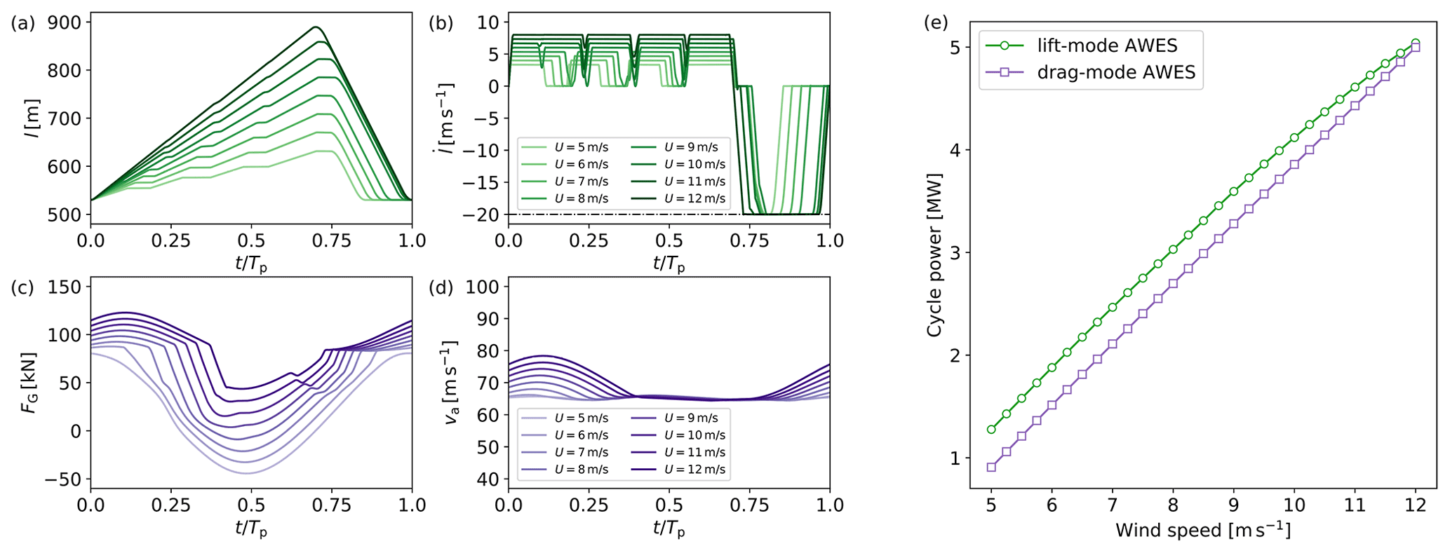
Figure 10Selected trajectory features (a–d) and power curves (e) of lift- and drag-mode AWE systems in region II. For lift-mode AWE systems, the wind speed dependency of tether length and reel-out speed are shown in (a) and (b). For drag-mode AWE systems, the wind speed dependency of generator thrust and apparent wind speed magnitude are shown in (c) and (d).
The effects of the reel-out strategy on wing–wake interaction can also be observed on the local flow conditions measured by the wing. Figure 9 shows the instantaneous streamwise wind speed component monitored at seven equidistant locations along the wingspan. For comparison, not that without interaction between the AWE system and the wind environment, wing sections would experience wind speeds in the range 9.7–10.9 m s−1. For the first reel-out strategy (see Fig. 9a), we observe large fluctuations of the instantaneous wind speed: sharp drops of the streamwise velocity components are measured during the lower part of the four power generation loops. These drops are particularly important for the entire starboard side (sections c000 to s030), suggesting that a large portion of the wing suddenly encounters a region of low wind speed that we can identify as the wake. Furthermore, the intensity of the velocity drop increases after every loop as the system reels out further downstream, indicating that the individual wakes of each loop are combined into a single wake. With the second reel-out strategy (see Fig. 9b), the patterns are less distinct and the magnitude of the fluctuations less significant, hence indicating that the interaction between wing and wake is limited. We still observe that the outer starboard part of the wing (sections s020 and s030) experiences sharp fluctuations, suggesting that the starboard wing tip flies through some wake region. However, these fluctuations are very local and temporary, while for the first reel-out strategy most of the wing is interacting with the wake.
Given the limited interaction between the wing and the wake when using the second reel-out strategy, i.e. with an induction-based upper limit of the reel-out speed, we will perform the lift-mode AWES farm simulation with the second design of lift-mode AWE system.
3.2.3 Operation of large-scale AWES in below-rated regime
When operating in a park, AWE systems are subject to large-scale wind speed variations and wakes of upstream systems. As a result, the operation of each individual system evolves as it experiences different wind conditions. Hence, we discuss here the effect of varying wind speed on the trajectories of drag- and lift-mode AWE systems. The power curves and selected metrics for the expected range of wind speeds 5.0 m s−1 ≤ UD ≤ 12.0 m s−1 are shown in Fig. 10, while the wind speed dependency of the flight path is shown in Fig. 3. A complete description of the effects of varying wind conditions on all system states, controls, and additional metrics is given in Appendix B.
For the expected range of wind speeds, the generated power ranges from approximately 1 to 5 MW for both operation modes. For lift-mode AWE systems, decreasing wind speeds mainly affect the reel-out patterns. At low wind speeds, the system only reels out, and hence generates power, during the downward part of the loops. In comparison, the upward flight is performed at constant tether length under fluctuating tether tension. Consequently, the increase in tether length during the reel-out phase is much more limited and hence the flight path more compact.
For the drag-mode AWE system, the shape of the single-loop flight path barely changes for varying wind speeds. However, the most noticeable difference is the contribution of the on-board turbines at low wind speeds. During the upward flight, the on-board turbines switch to propeller mode in order to overcome gravity and keep a constant flight speed and tether tension, and hence consume some power.
3.3 LES setup and AWES park layout
The turbulent ABL is modelled according to the procedure introduced in Sect. 2.1. In order to capture all the relevant spatio-temporal scales of the turbulent ABL in the precursor simulations and the wake effects in the AWE park simulations, the flow domain spans several kilometres and is resolved with high spatial resolution. The dimensions of the simulation domain are km3. The domain is discretised into cells of the size m3, resulting in a grid resolution of up to 80 millions cells for both main and precursor domains. The mean inflow velocity of main and precursor domains is Uref=10.0 m s−1 at 100 m altitude. Note that temporally resolved subsets of the generated precursor simulations are available for download from the Zenodo platform (Haas and Meyers, 2019).
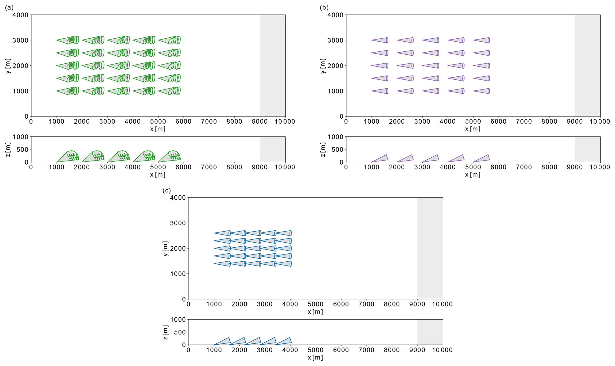
Figure 11Visualisations of top and side views of AWE park layouts in the main LES domain. (a) Lift-mode AWE park with layout 1 (L1), (b) drag-mode AWE park with layout 1 (D1), and (c) drag-mode AWE park with layout 2 (D2). The grey area represents the fringe region required for inflow recycling from the precursor simulation.
For the utility-scale deployment of their technology, Ampyx Power envisions park power densities in the range of 10–25 MW km−2 while targeting a system packing of about , where L is the maximal tether length (Kruijff and Ruiterkamp, 2018). Accordingly, we investigate three different AWE park configurations with the same packing density, where each park is composed of 25 systems ordered in five rows and five columns with an equidistant spacing between each system, i.e. L in the streamwise directions and in the spanwise direction. The top and side views of the three different AWE park layouts are shown in Fig. 11.
The first AWE park operates with lift-mode AWE systems, and the reference layout length is set to L=1000 m. This park layout is the densest possible layout to be operated with the designed lift-mode AWE system, such that the allocated areas do not overlap, and will further be referenced as L1 (lift-mode park 1). The second AWE park operates with drag-mode AWE systems and the same layout as L1 and is referenced as D1 (drag-mode park 1). These two AWE parks can achieve farm power densities up to 10.0 MW km−2 when all systems operate at rated wind speed. The third AWE park also operates with drag-mode AWE systems but with a reference layout length L=600 m. This AWE park, referenced as D2 (drag-mode park 2), corresponds to the densest possible layout for the designed drag-mode AWE system and can achieve a farm power density up to 27.8 MW km−2 in rated wind conditions. Note that the flight path constraints in Table 1 ensure a safe operation in accordance with the area allocated to each system in all park configurations. At the initial simulation time, the states of the AWE systems in the parks are initialised to the state values of the pre-computed reference trajectories for UD=10.0 m s−1.
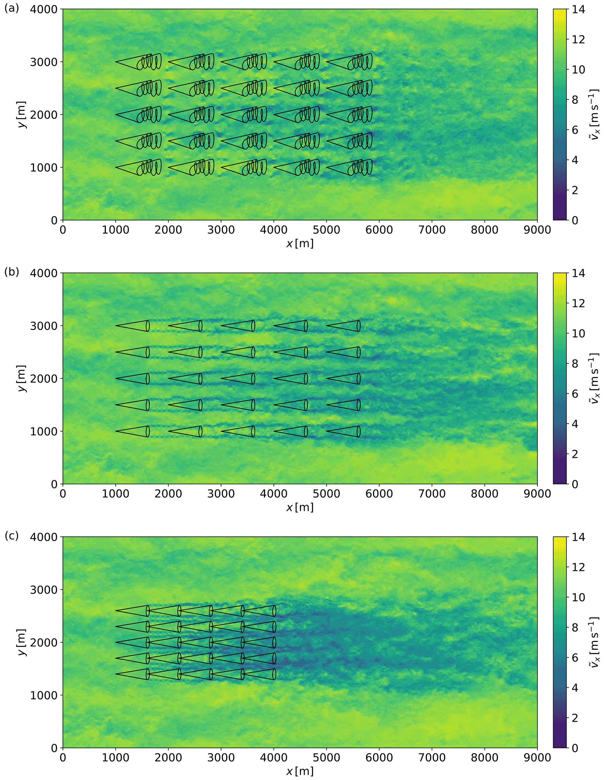
Figure 12Instantaneous snapshot of streamwise wind velocity through the horizontal xy plane at a height z=200 m for the AWE parks L1 (a), D1 (b), and D2 (c) at the end of the spin-up phase. The black lines depict the park layout by showing the horizontal footprint of the AWE system trajectories.
The simulations are performed on the high-performance-computing infrastructure of the Flemish Supercomputer Center (VSC). The computational cost of one LES time step typically largely exceeds the computational cost of one NMPC evaluation. Hence the required computational resources depend heavily on the grid resolution, which also limits the simulation horizon. However, given that AWES dynamics are faster than ABL flow dynamics, the control actions of each AWES are evaluated several times per LES time step. In total, 54 000 evaluations per AWES are performed during the simulation horizon of 4500 s. Consequently, the total execution time of the LES time step may depend on the execution time of individual NMPC evaluations. The performance of NMPC evaluations depends on several parameters, such as the length of the prediction horizon or the number of model variables. For drag-mode AWESs on the one hand, the execution time of NMPC evaluations is almost negligible, accounting on average for less than 5 % of the execution time of an LES time step. For lift-mode AWESs on the other hand, the execution time of NMPC evaluations can vary substantially. While about 95 % of the evaluations are performed in less than 1.0 s, similar to drag-mode AWESs, the remaining 5 % of the evaluations require about 15–30.0 s. This performance drop is generally observed when AWESs operate in heavily constrained regions of the variable space or transition between considerably different reference flight paths. As a result, the drag-mode AWE park simulations require about 1200 node hours (or 52 node days) while the lift-mode AWE park simulation requires about 1600 node hours (or 67 node days) on the Tier-2 hardware of VSC.
In the following section, we present the main outcomes of the simulations of AWE parks in the turbulent boundary layer. Figure 12 shows instantaneous snapshots of the streamwise wind velocity for the three park configurations investigated in this study. The figure illustrates the complexity of the flow, highlighting large-scale wind speed variations and large wake structures trailing behind individual AWE systems and how they affect the ABL flow at park level. First, we have a look at the time-averaged characteristics of the ABL flow in Sect. 4.1. Next, we investigate the behaviour of individual AWE systems subject to turbulent wind conditions and how their tracking and power performance are impacted in Sect. 4.2. Last, we discuss the power performance of the complete AWE parks and in particular how wakes impact their efficiency in Sect. 4.3.
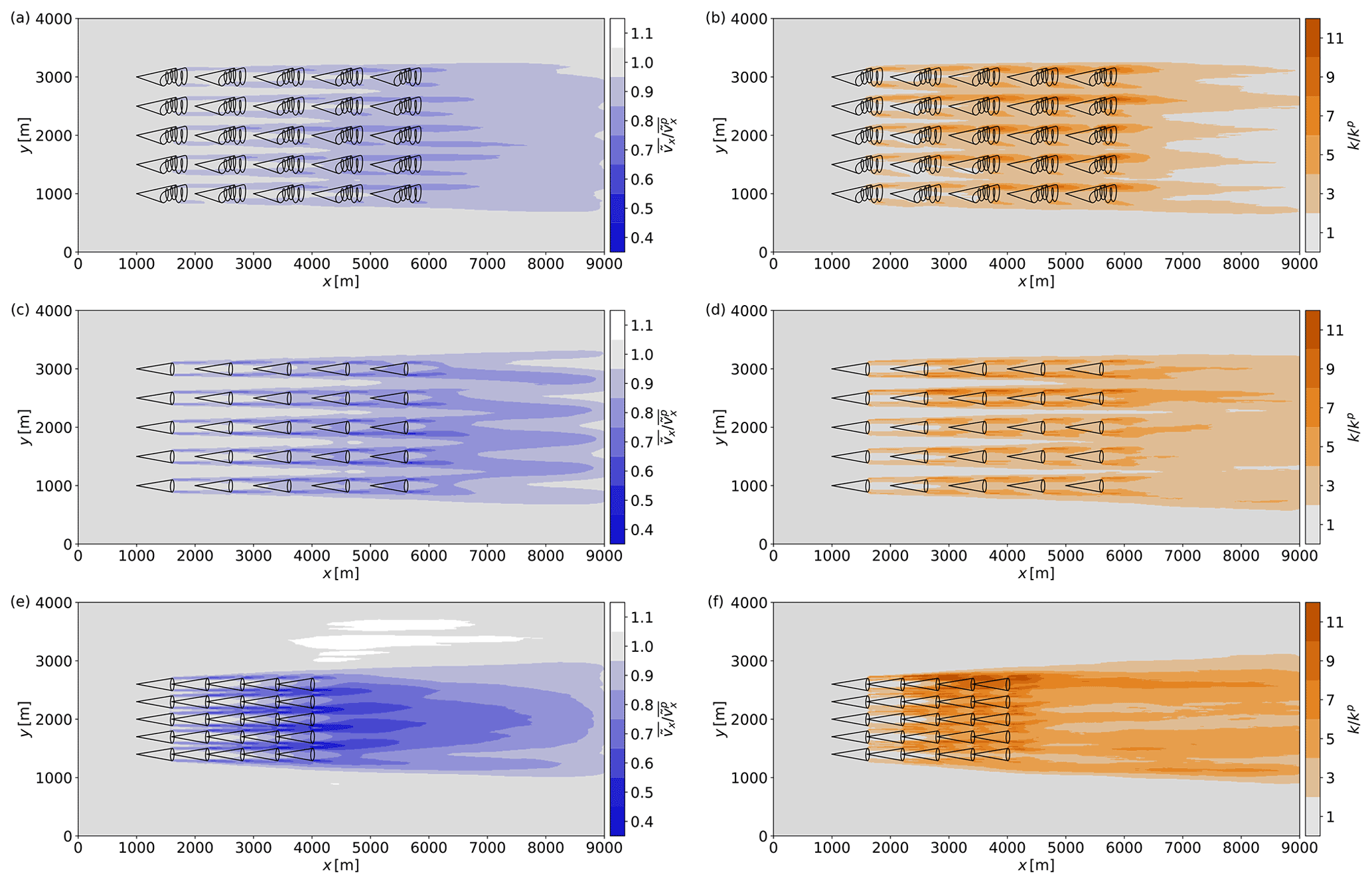
Figure 13Mean fields of streamwise wind velocity and turbulent kinetic energy shown in the horizontal xy plane at a height z=200 m for the AWE parks L1 (a, b), D1 (c, d), and D2 (e, f). The simulation is averaged over 1 h of park operation and normalised by the mean precursor values and . The black lines depict the park layout by showing the horizontal footprint of the AWE system trajectories.
To ease the comparison, the trajectories of the AWE systems are parameterised as a circular flight path centred around a virtual trajectory centre. For the lift-mode system, the diameter of the trajectory is approximately 240 m, and its centre is located 645 m downstream of the ground station at an altitude of 220 m. Equivalently, for the drag-mode system, the diameter of the trajectory is approximately 200 m, and its centre is located 610 m downstream of the ground station at an altitude of 190 m.
4.1 Time-averaged ABL flow statistics
4.1.1 Mean ABL flow characteristics
Figure 13 shows time-averaged contours of normalised streamwise velocity deficits and turbulent kinetic energy averaged over 1 h of AWE park operation. The wake field develops through the parks as individual wakes add up with the wakes induced by consecutive AWE systems. We observe in the three cases that downstream system rows operate in fully waked conditions. At the last row of the park, the mean velocity deficit, relative to the ABL precursor, reaches about 10 % for the lift-mode park (L1), while for the drag-mode parks the velocity deficit increases to about 20 % (D1) and up to 30 % (D2). In the trail of the annuli swept by the wings, these velocity deficits are further accentuated and can reach up to 20 % for the lift-mode AWE systems (L1) and respectively 40 % and 50 % for the drag-mode AWE systems (D1 and D2). For the drag-mode AWES park with dense layout (D2), the blockage effect of the drag-mode AWE systems also results in an acceleration of the mean flow up to 10 % around the park, which cannot be observed for the two AWE parks with moderate layout (L1 and D1).
The mean turbulence intensity TI of the current ABL simulation ranges between 2 % and 8 % and is about 3 % at operation altitude. Hence the power extraction and the wake mixing in the AWE park lead to large increases in turbulent kinetic energy (TKE) levels. The observed TKE levels can reach up the 10-fold of the precursor levels. In particular for lift-mode systems (L1), we observe higher levels of turbulence compared to the same drag-mode configuration (D1), possibly due to the merging effect of individual loop wakes discussed in Sect. 3.2.2. Furthermore, the lift-mode AWE systems sweep over a much larger area than the drag-mode AWE systems. For the latter in layout D1, the lateral extent of the wakes is more limited. Hence, individual columns of drag-mode systems accumulate the effects of their wakes in streamwise corridors, while the wakes spread much farther in the spanwise direction for the lift-mode AWE park (L1). The higher packing density of the second drag-mode AWE park (D2) exhibits the same phenomena as park D1 but with much higher intensity, given the reduced space available for wake recovery.
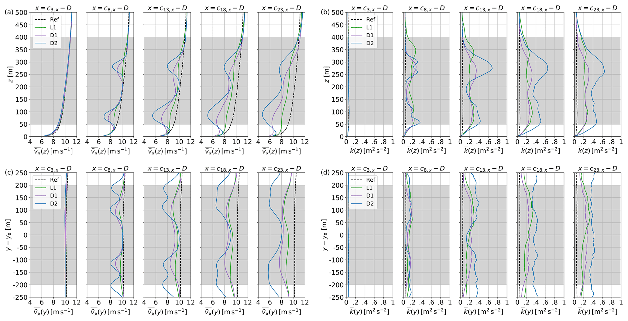
Figure 14Mean profiles of streamwise wind velocity and turbulent kinetic energy through the central park column (x=2000 m) for the AWE parks L1, D1, and D2. The vertical (a, b) and horizontal (c, d) profiles are shown one diameter D upstream of the trajectory centre ci of the five AWE systems. The black dashed lines show the precursor reference and the grey-shaded area the operation region of AWE systems.
4.1.2 Flow characteristics inside the parks
We can further deepen the analysis by looking at vertical and horizontal profiles of velocity deficit and turbulent kinetic energy as shown in Fig. 14. The profiles are shown one diameter upstream of the trajectory centre for AWE systems located in the central column of the parks. For the lift-mode system, the diameter of the trajectory is approximately 240 m, and it is located 645 m downstream of the ground station at an altitude of 220 m. Equivalently, for the drag-mode system, the diameter of the trajectory is approximately 200 m, and its centre is located 610 m downstream of the ground station at an altitude of 190 m.
The profiles provide an overview of the local flow distribution experienced by each system in downstream locations of the AWE column. The profiles confirm the prior observations relative to the downstream development of the wakes through the park: for the lift-mode AWE park, the wake is much more widespread and therefore induces a weaker velocity deficit. In contrast, for drag-mode AWE parks, the wake exhibits more localised and stronger velocity deficits, highlighting the annular shape of the wake. Each park configuration shows higher velocity deficits at the bottom half of the loops, induced by higher loadings on the wing. In addition, wake recovery in the upper part of the loop is eased by higher turbulence levels.
The wake impacts are much stronger for the drag-mode AWE park (D2) with a higher packing density. The horizontal profiles show that the wake merges with the wakes of neighbouring AWES columns as its radius extends laterally the further downstream it progresses. Hence, wakes do not only aggregate as they advect downstream but also merge in the spanwise direction, therefore resulting in the stronger velocity deficits and higher TKE levels observed for the higher farm power density.
4.2 AWES operation in turbulent boundary layer
AWE systems operate in very different wind conditions depending on the operation mode, the park layout, and their own position within the park as seen in the previous section, Sect. 4.1. In this section, we discuss how these parameters affect the operation of the systems, in particular how they adapt their respective trajectories and how accurately the NMPC can track their flight path.
Figure 15 shows the reference wind speed of the trajectories tracked by the AWE systems as directed by the supervision level of the controller. Each reference trajectory is tracked for the duration of respectively one cycle for lift-mode systems (≈65 s) and five cycles for drag-mode systems (≈50 s) before it is updated by the controller based on the averaged velocity sampled by the wind speed estimator over that time period. In particular, we show the tracking behaviour of the five rows of AWE systems of the central column of the three park configurations.
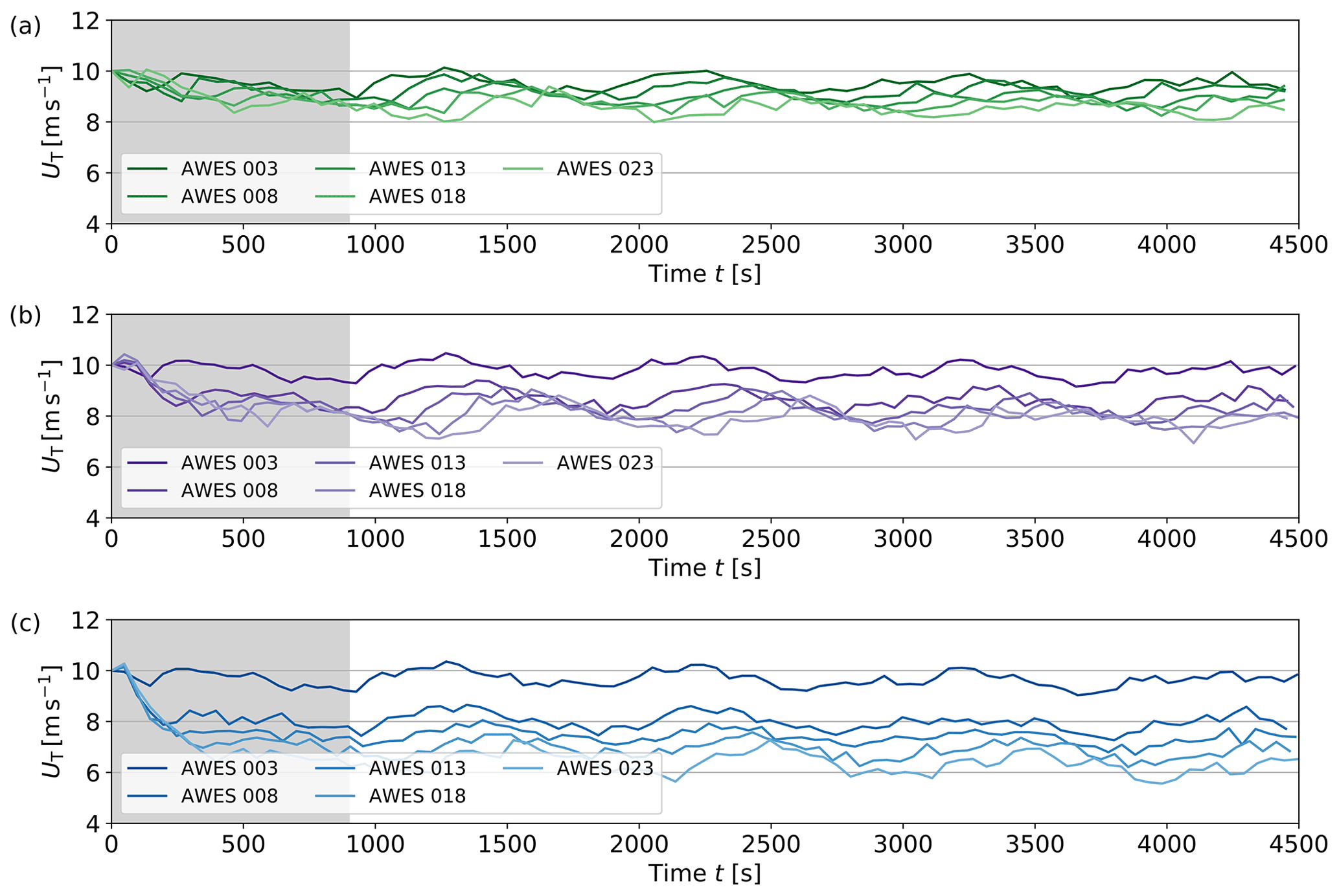
Figure 15Time series of reference wind speed tracked by the five AWE systems of the central park column (x=2000 m) for the AWE parks L1 (a), D1 (b), and D2 (c). The grey shaded area covers the spin-up phase of the park simulations.
At the start-up of the operation, each system experiences similar conditions from the unperturbed ABL flow. As systems begin to harvest power and induce their own wakes, upstream wakes travel downstream and start to impact the operation of downstream rows until the complete park operates in fully waked conditions at the end of the spin-up phase at t=900 s. The variations in the tracked value for the front row AWE system (AWES 003) are due to the inherent unsteadiness of the ABL flow. We observe how these large-scale wind fluctuations experienced at the front row propagate with some delay through the downstream rows of the park. However, the large decreases in tracked speed for the downstream systems are due to the effects of upstream wakes. As discussed above, drag-mode AWE systems experience much stronger wakes and hence track lower wind speeds than lift-mode AWE systems. In particular, a larger decrease is observed from the front row to the second row.
Note that the amplitude of the large-scale variations in the ABL varies from one column to another. Consequently, the different columns of the parks do not operate similarly and impose a different forcing on the ABL flow field. This effect can explain the asymmetry observed in the time-averaged quantities shown in Fig. 13. In particular, the averaging period of 1 h may not be sufficient to entirely smooth out these temporal and spatial variations across the entire AWE farms.
We can further look at the instantaneous streamwise wind speed measured in flight at the wing as shown in Fig. 16 for two systems located in the front and back rows. Despite the ambient turbulence of the ABL flow, the wind speed monitored by the front-row systems coincides quite well with the reference wind speed distribution of the tracked trajectories. However for the lift-mode system, we observe additional sharp fluctuations resulting in abrupt increases and decreases in the monitored streamwise wind speed. These effects are amplified as the system progresses further in the reel-out phase, as seen in the time window s]. This indicates that the wing may still interact with its own wake in some sections of the flight path. In order to ensure a reliable operation, the reel-out speed limitation was lifted off for flight path tracking to allow a better reactivity of the systems to the unsteady wind conditions. Hence, the systems can achieve higher reel-out speeds than the reference.
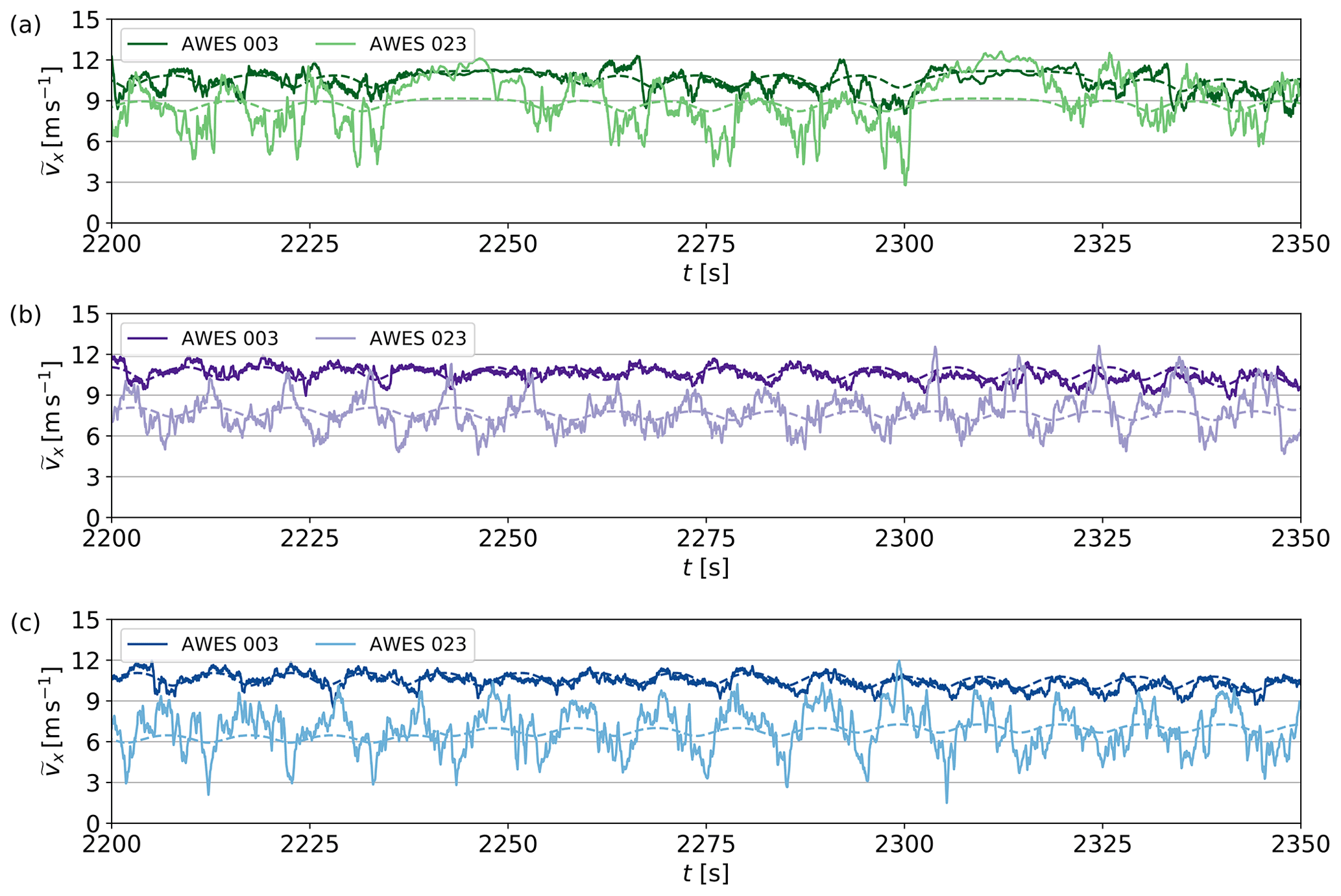
Figure 16Time series of streamwise wind speed monitored by the front and rear AWE systems of the central park column (x=2000 m) for the AWE parks L1 (a), D1 (b), and D2 (c). The coloured dashed lines show the reference quantities of the tracked trajectories.
The strong velocity deficits and the higher levels of TKE observed in the back rows of the parks greatly impact the instantaneous wind speed monitored. We observe a much larger range of fluctuations for AWE systems located in the last row than in the first row. The effects described for the front row lift-mode system are accentuated for the back row system, suggesting the presence of compact wake regions from upstream systems advecting through the park.
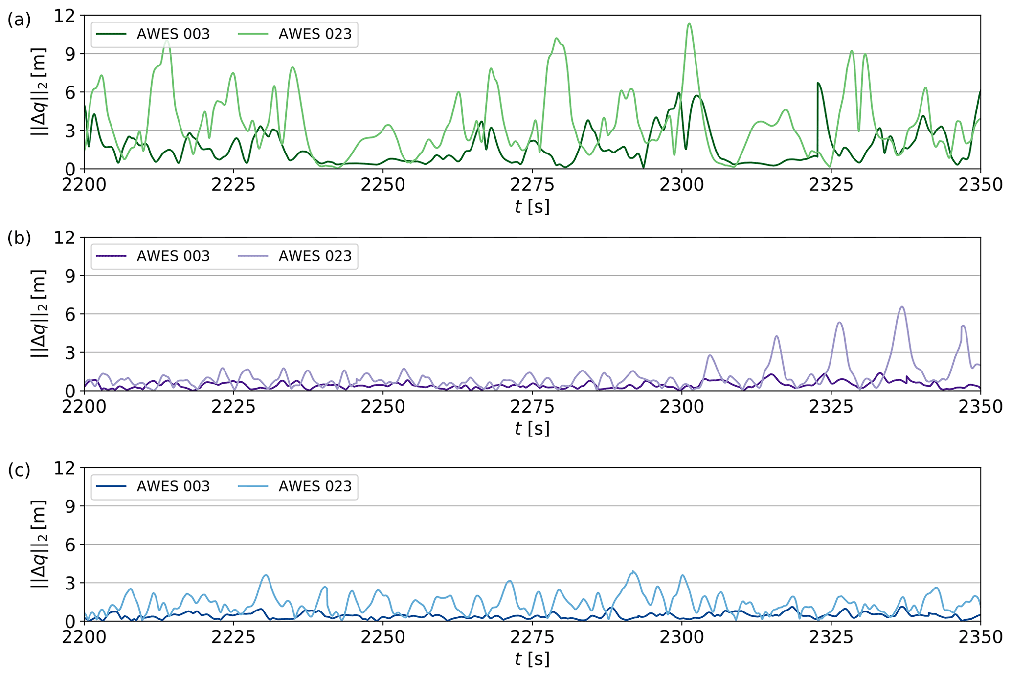
Figure 17Time series of position offset monitored by the front and rear AWE systems of the central park column (x=2000 m) for the AWE parks L1 (a), D1 (b), and D2 (c).
The unsteady wind conditions also impact the tracking accuracy of the NMPC. Figure 17 shows the position offset of the systems relative to the tracked flight. For the drag-mode systems operating in the front row of parks D1 and D2, the tracking error is almost negligible. This error increases for the systems in the back row as they experience larger wind speed fluctuations. For the lift-mode park L1, we observe larger position tracking error, partly due to the additional degree of freedom related to the reel-out and reel-in of the tether. The highest offsets occur however after the AWE system flies through a low-wind-speed region. Nevertheless, the error remains marginal compared to the dimensions of the flight path, as it rarely exceeds 12 m. Hence, the NMPC algorithm tends to always react reliably to the wind speed fluctuations and steers the system back onto its reference flight path.
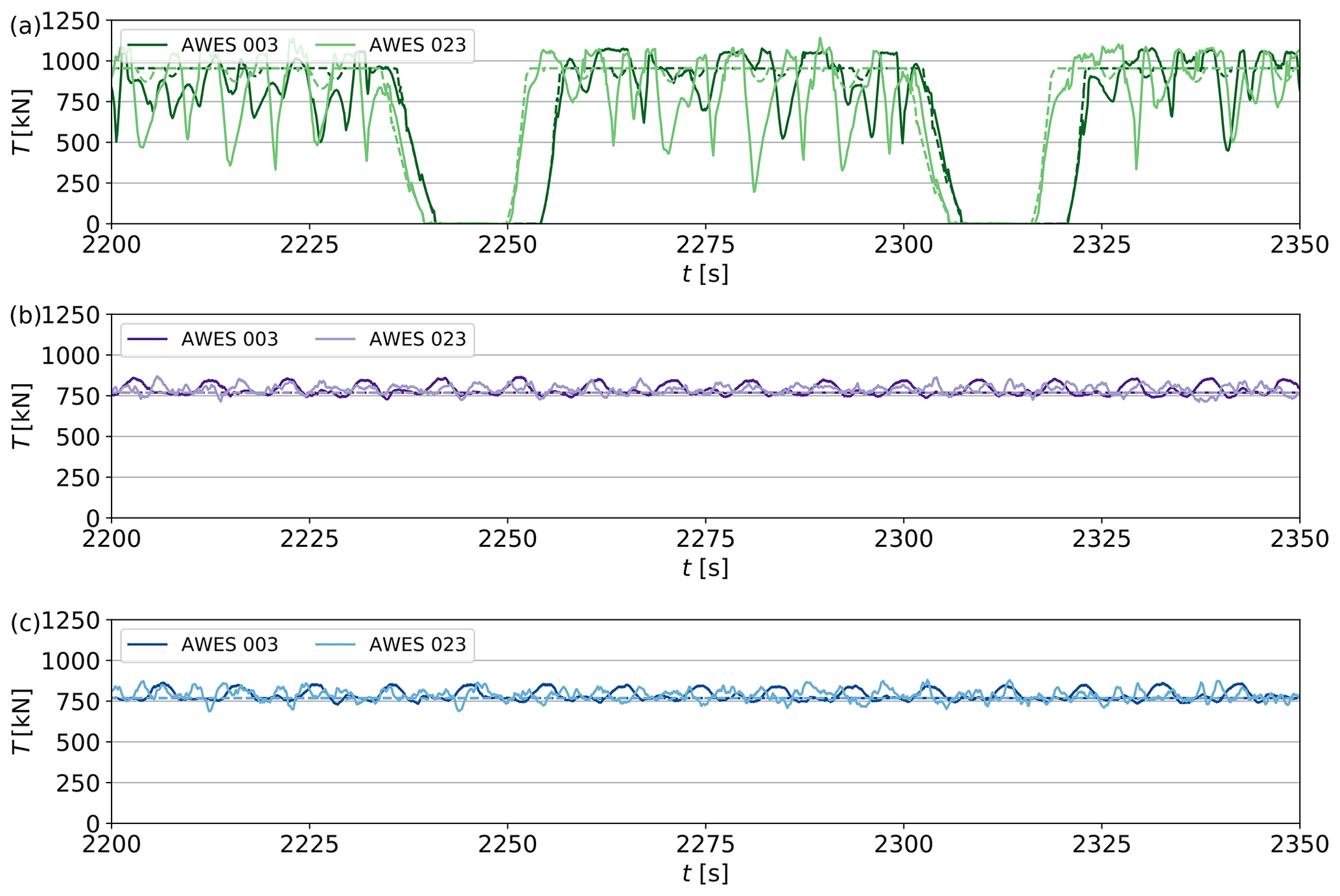
Figure 18Time series of tether tension TT monitored by the front and rear AWE systems of the central park column (x=2000 m) for the AWE parks L1 (a), D1 (b), and D2 (c). The coloured dashed lines show the reference quantities of the tracked trajectories.
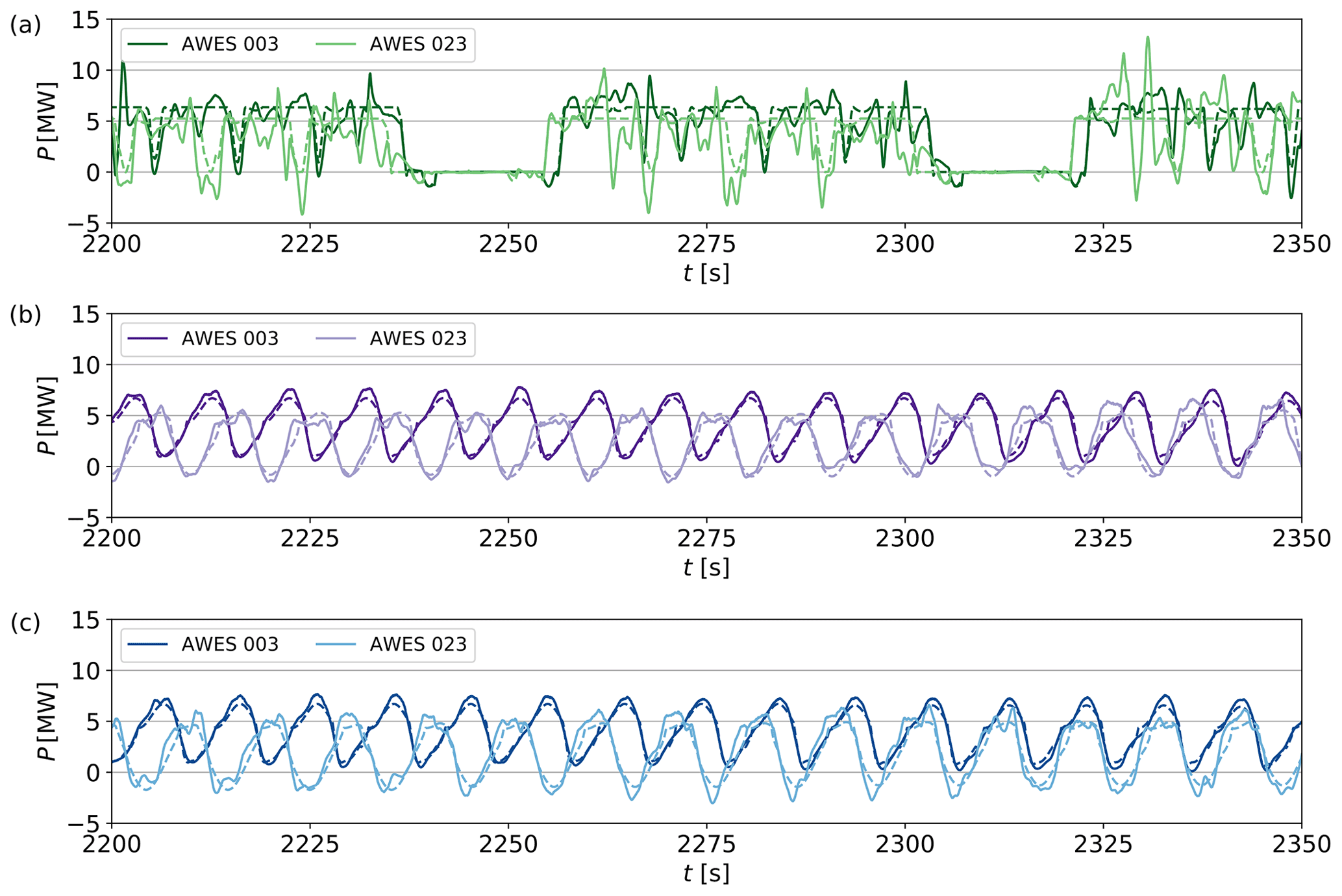
Figure 19Time series of mechanical power P monitored by the front and rear AWE systems of the central park column (x=2000 m) for the AWE parks L1 (a), D1 (b), and D2 (c). The coloured dashed lines show the reference quantities of the tracked trajectories.
4.3 Power performance at system and park level
The unsteady wind conditions not only affect the tracking behaviour of each AWE system but also impact their performance. Figures 18 and 19 respectively show the tether tension and mechanical power of the front and back row systems in the central column of the parks. For the lift-mode systems, the low-speed regions crossed by the wing generally lead to a drop of the tether tension that must be compensated for by steering manoeuvres. These tether tension variations negatively impact the amount of generated mechanical power such that we observe power losses of about 10 % to 15 % relative to the reference power of the tracked trajectories. For the two drag-mode park configurations, the wind fluctuations barely impact the operation of the systems, and we observe a good tracking of the power generation profiles. In the back row however, the tracked flight path and the low wind speed available require the on-board turbines to operate as propellers in order to overcome gravity while flying upward. Hence, some drag-mode systems end up also consuming some of the harvested power. Note that the tether tension maxima monitored at each system match the relaxed upper bound used for flight path tracking as discussed in Sect. 2.4.
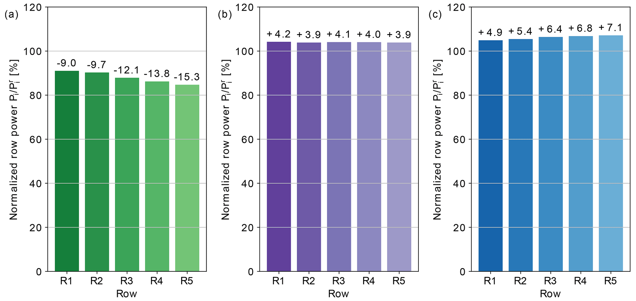
Figure 20Mean row power averaged over 1 h of park operation and normalised by tracked reference power for the AWE parks L1 (a), D1 (b), and D2 (c).

Figure 21Mean row power averaged over 1 h of park operation and normalised by front row value for the AWE parks L1 (a), D1 (b), and D2 (c).
We further address the power extraction process from the perspective of the complete AWE park, and in particular from the system location in the park. Figure 20 shows the mean power generation of each row relative to the reference power of the tracked trajectories for the three different park configurations. In this way we can quantify the power losses due to local wind speed fluctuations and the steering efforts they cause. For the lift-mode park, every system across each row is only capable of harvesting a fraction of the tracked power. While in the front row up to 91 % of the tracked power can be harvested, the efficiency of the power tracking decreases gradually for the downstream rows, such that approximately 85 % of the tracked power can be harvested in the last row. For the drag-mode AWE parks, individual systems are able to harvest more power from the wind than expected. For the drag-mode park D1, each row harvests on average about 4 % more power. With the denser layout (D2), the systems in the front row harvest 5 % more power while this increases to up to 7 % in the last row. This suggests that the supervision level underestimates the local wind conditions experienced by the systems.
Figure 21 shows the mean power generation of each row relative to the front row of the farm. This allows us to quantify the wake-induced power losses for the three different park configurations. For the lift-mode AWE park, the relative power decreases through the farm; i.e. the power deficit between front row and downstream rows reaches up to approximately 17 %. For the drag-mode AWE parks, the wake losses are much more important and reach approximately 25 % in the last row of AWE park D1 and up to 45 % for AWE park D2 with a denser layout. While for the lift-mode AWE park the power decrease across the subsequent rows is progressive, for drag-mode AWE parks, the power losses increase abruptly between the first and second rows. This drop accounts for about 62 % and 52 % of the row losses for the park configurations D1 and D2 respectively.
In this study we have investigated the wake interaction and power extraction for large parks of utility-scale AWE systems. Flight path tracking by means of model predictive control (MPC) has proven to be a robust control strategy for both lift- and drag-mode systems when operating in turbulent wind conditions: the path tracking results in position offsets generally up to 12 m, while satisfying the set variable bounds and tracking the power profiles quite accurately, in particular in drag mode. Lift-mode AWE systems encounter however important fluctuations in local wind speeds during operation, which can lead to temporary large decreases in tether tension and significant reductions of instantaneous power. First, we have observed that lift-mode systems can interact with their own wake: during reel-out, the wing can fly (partially) through or in the direct vicinity of the wake induced in the previous power-generating loops. Hence, the interaction with its own wake needs to be considered already during the design phase: when generating optimal reference trajectories, it is crucial to define reeling strategies that avoid these situations and incorporate induction phenomena in the modelling procedure. This is an active topic in current AWE research. Second, these large wind speed fluctuations can be associated with the characteristic wakes induced by lift-mode AWE systems: while the flow forcing is negligible during the retraction phase, the wakes induced during consecutive loops of the power generation phase tend to merge into a single-wake structure. This interaction leads to compact, low-speed flow regions which get advected downstream with the mean flow and negatively impact the operation of downstream systems.
Moreover we showed that for the three investigated configurations, wake effects and wake-induced losses in utility-scale AWE parks are significant. The induced wakes display very characteristic annular shapes; however the strength and the width of the wakes highly depends on the operation mode and the park layout. In terms of park performance, we observed wake-induced performance losses of up to approximately 15 % in the last row for the lift-mode AWE park. For the two drag-mode AWE parks with moderate and dense farm power densities, the wake-induced power losses increase up to 25 % and 45 % respectively in the last row of the parks. Hence, the layout of the farm also plays a considerable role in the performance of the park. However, note that wake losses and tracking losses/gains can not completely be isolated from each other: improving the tracking behaviour of lift-mode systems by limiting the large tension fluctuations in the tether would result in a stronger axial flow induction, hence leading to larger wake losses and vice versa.
The current predictions formulated in this study can be refined by increasing the resolution of the LES flow domain. With a higher grid resolution, the representation of the individual AWE systems can be enhanced, limiting their forcing effects to the direct vicinity of the wing instead of large sectors. The estimation of the aerodynamic quantities along the wingspan of the aircraft would also benefit from higher resolutions as a larger range of turbulent motions are resolved, hence increasing the modelling accuracy of the wing behaviour. However, increasing the grid resolution is not the only approach to improve the accuracy of the framework. The fully coupled computational framework integrates numerous building blocks into a single simulation platform with a high level of complexity. The overall fidelity of the simulations can however be improved in the future by increasing the complexity of individual components of the framework and addressing the following known limitations: first, we can improve the modelling of the atmospheric boundary layer. The description of the ABL flow can be enhanced by including Coriolis forces and thermal effects in the LES framework (Allaerts and Meyers, 2015). The inclusion of these effects significantly modifies the structure of the flow, in particular capturing the inversion layer separating the turbulent boundary layer from the free atmosphere above. The height of the inversion layer, the strength of wind veer in the boundary layer, or the occurrence of low-level jets will certainly affect the flight path characteristics of AWE systems, such as optimal heights and tether length. These effects will further impact the controllability and power performance of the systems and hence require further investigations. Second, the complex dynamics of AWE systems can be better characterised by more detailed models. One possible alternative to the point-mass model is the 6DOF rigid-body model (Malz et al., 2019). This model includes the rotational dynamics of the complete system, hence removing the need for a state-based assumption of the wing orientation and further providing a more accurate prediction of the flight manoeuvres. In addition, this model includes realistic control capabilities by steering the aircraft using the deflection of control surfaces such as ailerons, elevators, and rudders. Third, the modelling of the tethered aircraft can further be improved by incorporating unsteady aerodynamics. Fast pitching manoeuvres of the wing and sharp turns of the aircraft can have considerable effects on the local aerodynamic characteristics of the wing sections and hence have a significant influence upon the resulting aerodynamic forces of the system. Additionally, the aero-elastic response of the aircraft to the unsteady loading should be considered in order to prevent fatigue of the structure. Although the rigid-rod assumption performs well for the high-tension power generation phases (Malz et al., 2019), this model does not capture the tether dynamics. The incorporation of tether sag (Trevisi et al., 2020) would benefit the completeness of the modelling effort.
In terms of tracking performance, the improved system modelling should help reduce the mismatch between model and virtual plant such that an enhanced NMPC algorithm could accurately track the flight path while considering the integrated lifting line forces to compute the AWES dynamics. Also, in order to further improve the closed-loop performance of the systems in terms of power output, one can consider applying approximate or exact economic NMPC formulations instead of the pure flight path tracking scheme used in this study.
Finally, the wake profiles show quite large deviations from the logarithmic mean flow distribution assumed by the high-level controller. Therefore in the future, we can implement supervision strategies that take the wake shape into consideration and make use of the inherent flexibility and adaptability of AWE systems: we can further use the wake profiles to generate new optimal flight trajectories in which individual systems adapt the elevation and azimuthal angles of operation to eventually avoid the upstream wakes.
To conclude, this study demonstrates the considerable interaction between large-scale AWE systems and the atmospheric boundary layer for the considered park configurations and motivates further investigations to achieve an efficient operation of utility-scale AWE parks.
Ahead of the investigation of utility-scale AWE parks, we have conducted a series of single-AWES analyses in order to assess the computational setup used in this study. In this appendix, we address in particular the tuning of the actuator parameters in Sect. A1, the detailed analysis of wake structure by means of high-resolution simulation in Sect. A2, the grid dependency of wake characteristics in Sect. A3, and finally the convergence of the supervision level of the controller in Sect. A4.
Figure A1 shows the computational setup used in this study of both lift- and drag-mode AWE systems. The domain dimensions are [m3]. We use three different resolutions to discretise the flow domain as specified in Table A1. The AWE systems operate in a sheared inflow without ambient turbulence parameterised by a logarithmic profile given in Eq. (27), where Uref=10.0 m s−1.
A1 Tuning of actuator parameters
The dependency of the actuator line and actuator sector methods to their (temporal) parameters is investigated for the simulation of a single drag-mode AWE system. The system operates at a reference trajectory m s−1, and the flow domain is discretised using the finest grid resolution with cell size m3. The filter width of the Gaussian filter is uniform in all three spatial directions and is set for all actuator methods to Δf=2Δx following the recommendations in Troldborg et al. (2010).
The chosen grid resolution requires a minimal simulation time step Δt=0.1 s. Accordingly, we test three ALM simulations with LES time steps of Δt=0.1 s, Δt=0.05 s, and Δt=0.025 s and three ASM simulations with time step Δt=0.1 s and filter constants τf=1Δt, τf=2Δt, and τf=3Δt. The states of the AWE system are interpolated from the OCP reference, and the local aerodynamic quantities of each wing section are computed using the lifting line method presented in Sect. 2.2.2.
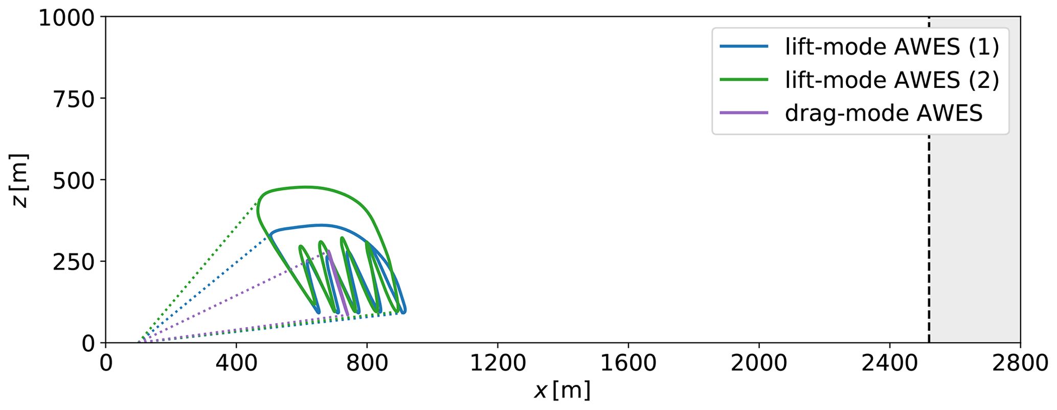
Figure A1Side view of the computational setup of the single-system simulations used for the analysis of lift- and drag-mode AWE systems.
Table A1Resolution of the computation domain [m3] with fine, medium, and coarse grids for the analysis of single AWE systems.
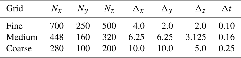

Figure A2Instantaneous angle of attack monitored at the wing tip section on the port (a) and starboard (b) sides. (c) Magnitude of the specific forces added to the flow field at the fourth stage of the LES Runge–Kutta scheme by means of actuator methods for different sets of parameters. Three ALM simulations are performed with different LES time steps, and three ASM simulations are performed with three different time filter constants. The black dashed lines show the OCP references.
Figure A2 shows time series of the angle of attack, measured at the wing tip sections, and of the specific aerodynamics forces added onto the flow. The ALM simulations exhibit large fluctuations of the added forces due to the varying flow conditions experienced by the wing. Within one LES time step, the local flow conditions monitored by individual wing section vary greatly due to the very localised effects of the ALM forces. The ASM simulations, on the other hand, weight the individual force contributions at discrete AWES time steps, hence resulting in smoother force distribution, while introducing a slight time delay, but also smoother variations in angle of attack in time given the low velocity gradients encountered due to the wider smearing of the forces onto the LES domain. The forces of the optimised reference trajectory using the point-mass model are shown for comparison: over the period of one full periodic cycle, the model mismatch between the forces computed with actuator methods and the reference OCP forces is less than 4 %.
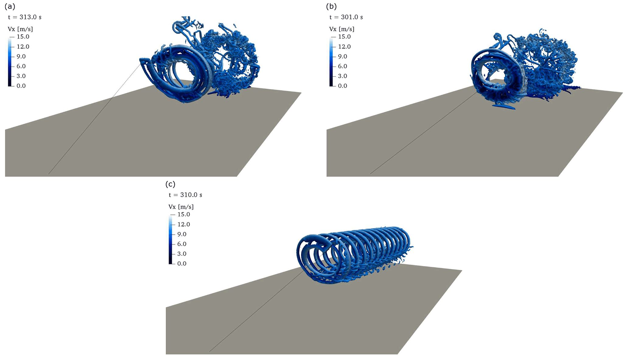
Figure A3Instantaneous frontal snapshots of the wake field of reference lift- and drag-mode AWE systems operating in an unperturbed logarithmic inflow at a wind speed UD=10 m s−1. Isovolumes of positive Q criterion, coloured by streamwise velocity for (a) the lift-mode AWE system with induction-based limitation of reel-out speed at t=313 s, (b) lift-mode AWE system with original bounds at t=301 s, and (c) drag-mode AWE system at t=310 s.
Given the high flight speed of the system, the wing navigates through several grid cells during one time step for the simulations with Δt=0.1 s and Δt=0.05 s. Therefore, the ALM requires the smallest time step, Δt=0.025, to ensure a smooth transition as the wing sweeps across the flow domain. This results however in a 4-fold increase in the computational effort. The ALM simulation with Δt=0.025 hence serves as a reference simulation. The ASM technique can be applied to simulations with Δt=0.1 and allows the approximate reproduction of the unsteady forcing of the reference ALM with an error less than 2 %. Increasing the value of the time filter constant τf tends to reduce the error but also increases the computational cost. Hence, in order to keep a reasonable computational cost and achieve a sufficient accuracy, we perform further AWE simulations with the ASM techniques using τf=2Δt.
A2 High-resolution simulations of single AWESs
We can extend the previous high-resolution simulations of a single drag-mode AWE systems to lift-mode AWE systems in order to investigate the structure of the wake flow and loads acting on the wing.
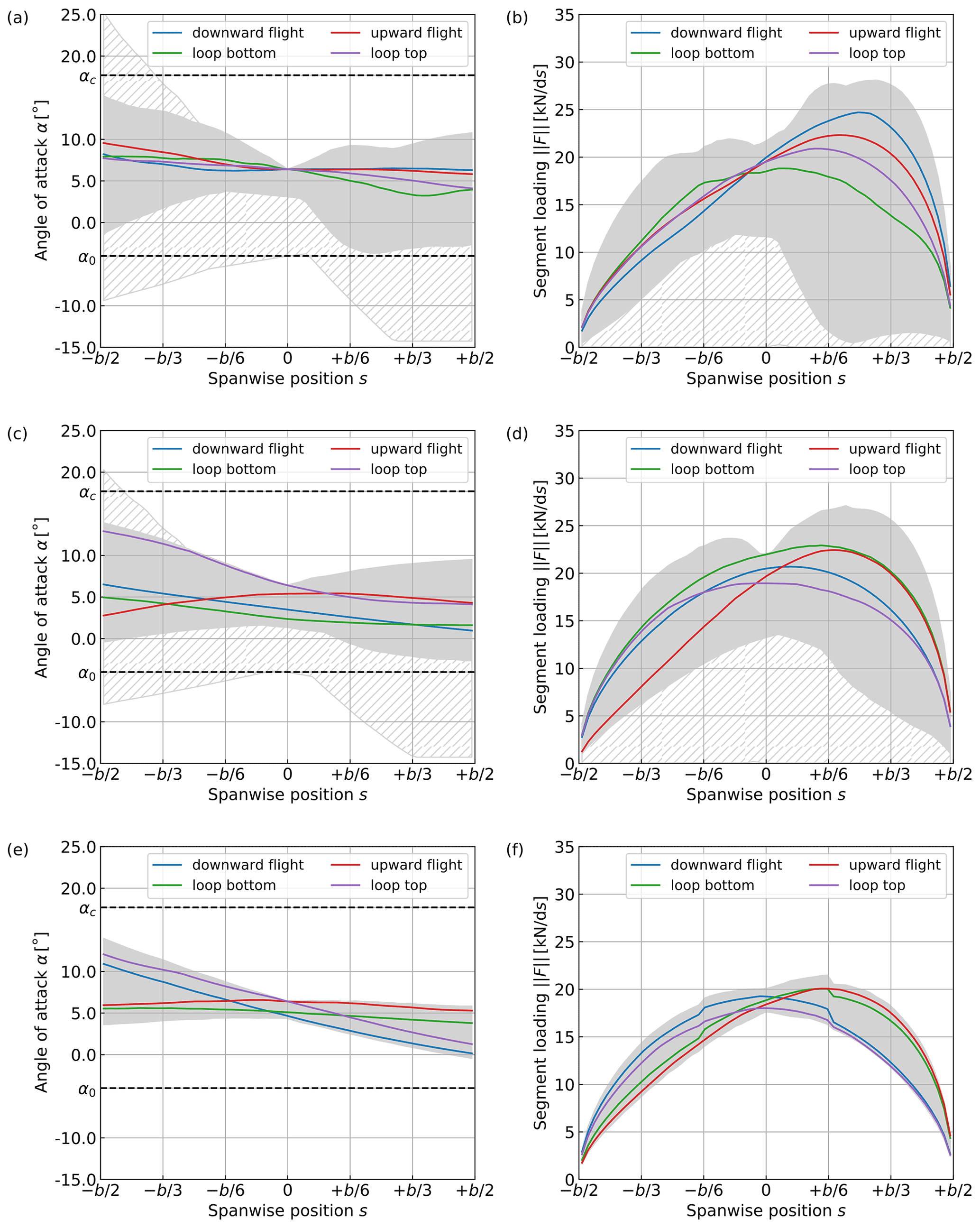
Figure A4Distributions of angle of attack and wing loading along the wingspan of (a, b) the lift-mode AWE system with original bounds, (c, d) the lift-mode AWE system with induction-based limitation of reel-out speed, and (e, f) the drag-mode AWE system. The coloured lines show the distributions at selected stages of the trajectories. The grey shaded areas show the value range during power generation while the hashed areas only show the reel-in phase.
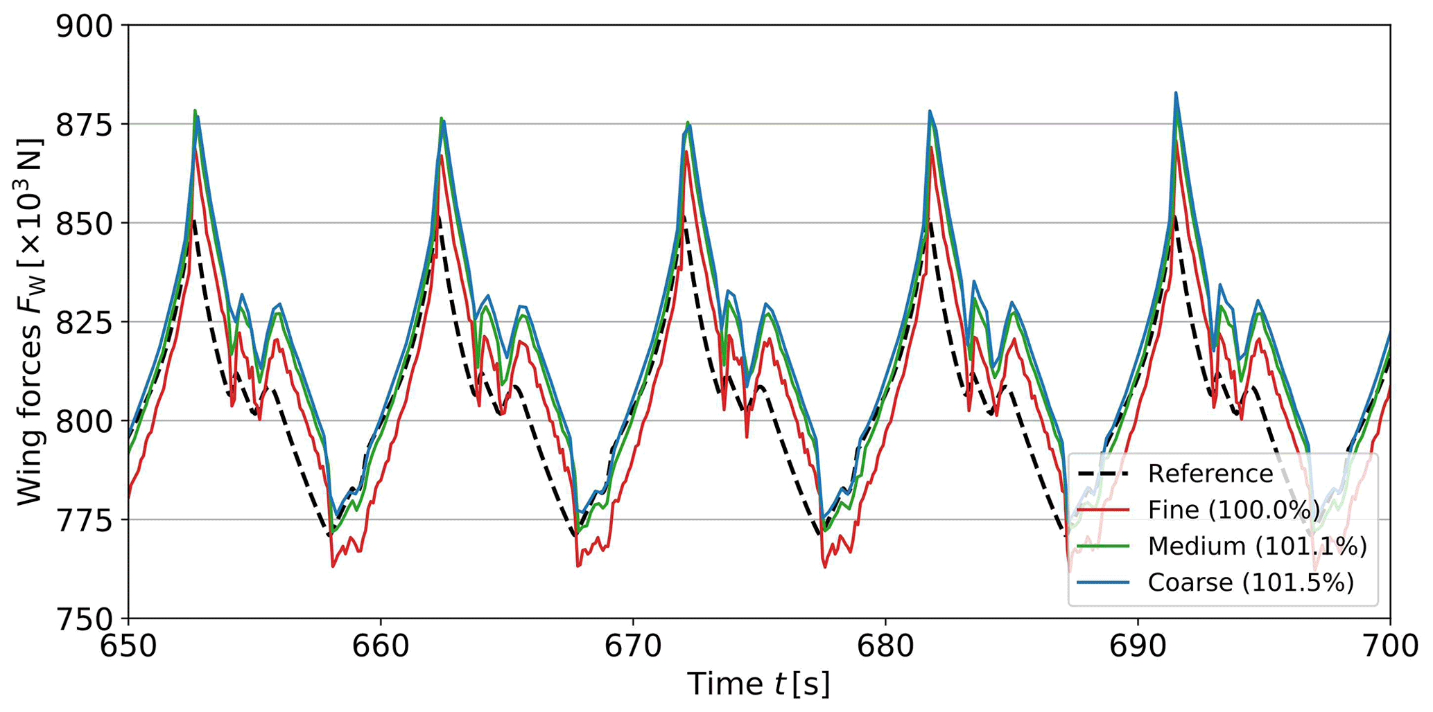
Figure A5Time series of integrated wing forces acting on the drag-mode AWE system for three different grid resolutions. The black dashed lines show the OCP reference.

Figure A6Time-averaged vertical profiles of streamwise wind velocity (a) and turbulent kinetic energy (b) at several locations downstream in the wake of the AWE system for three different grid resolutions. The black dashed lines show the inflow velocity profiles, and the grey-shaded area represents the operation region of AWE systems.
Figure A3 shows the structure of the wake flow for each AWE system simulated with ASM on the fine grid by visualising positive levels of Q criterion (Jeong and Hussain, 1995). For the drag-mode AWE system, tip vortices emanate continuously from the wing tips and are transported downstream in a coherent manner by the background flow. For the lift-mode AWE systems, the wing tip vortices generated during the individual loops start to interact with each other in the wake and eventually merge into a more significant single structure, which eventually breaks down further downstream due to the effect of mixing. The pumping behaviour of the lift-mode systems is also clearly visible: during the retraction phase, the aircraft takes a different path while being subject to a much smaller wing loading, hence interrupting the wake generation for a short amount of time. The grid resolution and the actuator settings enable us to resolve individual flow structures and provide interesting insights into the complex characteristics of the wake flow of single AWE systems.
Figure A4 shows the spanwise distribution of angle of attack and wing loading for the three different systems. During power generation, the angle of attack is kept below the critical angle of attack. For the lift-mode AWE systems, the wing tips stall briefly during the turn manoeuvre, initiating the reel-in phase. This effect is reduced when using the induction-based limitation of the reel-out speed and lasts less than 1 s without significantly modifying the total aerodynamic force acting on the wing. The force distribution along the wingspan is not elliptically distributed, as opposed to the assumptions of the point-mass model: the starboard side of the wing, the wing half flying at the outer side of the flight path, experiences a stronger wing loading than the port side due to the wing angular velocity, in particular during upward flight. For the drag-mode AWE system, the additional loading of the on-board turbines only slightly modifies the spanwise load distribution of the wing, in particular during the downward path of the loop.
A3 Analysis of grid dependency
Next, we perform the simulation of the single drag-mode AWES and assess the time-averaged flow quantities using the three grid resolutions specified in Table A1. In this grid analysis, the ratio of filter width to grid size is kept constant; hence . The simulation with the fine grid, which explicitly captures the individual tip vortices during the reel-out phase of lift-mode AWE systems, is considered the reference simulation.
Figure A5 shows time series of the aerodynamic wing forces integrated over its wingspan acting on the drag-mode AWE system for the three grid resolutions. The decrease in grid resolution comes with a simultaneous increase in the simulation time step, hence drastically reducing the computational expense of the simulations. This comes however at the cost that the larger spatial filtering and temporal smoothing result in a much wider sector, representing the wing more as a blunt body in the LES domain. The wide spread of the added forces in turn reduces the accuracy of the local aerodynamic quantities of each wing section compared to the reference simulation. Nevertheless, the integrated forces overestimate the reference by less than 2 % such that lower grid resolution can still sufficiently capture the resulting aerodynamic forces in order to accurately compute the AWES dynamics.

Figure A7Convergence of the controller supervision level for the three types of AWE systems investigated. The markers display the time-averaged wind speed value sampled during one (lift mode) and five (drag mode) periodic cycles, and the dashed lines show the associated reference wind speed of the tracked trajectories in increments of 0.25 m s−1.
Figure A6 shows time-averaged profiles of axial flow velocity and turbulent kinetic energy at different locations in the wake of the drag-mode AWE system for three different grid resolutions. The velocity profiles show that all resolutions can capture the general annular shape of the wake and its strength up to 1200 m behind the system. This good agreement allows us to use the coarse grid resolution for the AWE park simulations, where the downstream spacing between two rows of AWE systems does not exceed 1000 m and which would be too computationally expensive to perform on the finer resolutions. In terms of resolved turbulent kinetic energy, the medium and coarse grids cannot capture the same levels of turbulence as the fine grid. This is however less crucial given that in the fully turbulent ABL simulations, ambient turbulence triggers wake breakdown and turbulent mixing earlier than in the turbulence-free sheared inflow investigated here. While for the coarser resolution it cannot be assured that lift-mode AWE systems, even with the induction-based reel-out speed limitation, will not interact with their own wakes, this effect will be weakened given that the force smearing also reduces the strength of the tip vortices.
A4 Convergence of supervision level
Finally we can also verify the convergence of the supervision level of the controller and assess the different reel-out strategies employed for the lift-mode systems. Figure A7 shows the tracking profiles of the three AWE systems by the time-averaged wind speed values sampled by the controller and the associated reference velocity of the tracked trajectories. All systems show good convergence towards an asymptotic value between 9 and 10 m s−1. As discussed in Sect. 3.2.2, lift-mode AWE systems may interact with their own wakes; therefore we have used two different reel-out strategies. Figure A7 shows that the induction-based reel-out strategy used by the lift-mode system (1) allows us to track higher wind speed references, showing that the wing experiences less interaction with its wake. Therefore, this strategy also allows us to operate the system along trajectories generating more power and hence increases the performance of the AWE park.
The virtual flight data of each individual AWE system, including all states and controls, are monitored for the different AWE park simulations. The monitored flight data, the tracking scheme of each AWE system, and the tracked reference trajectories of the AWE systems, are openly available on the research data repository Zenodo from the dataset “Large-eddy simulations of airborne wind energy farms: AWES virtual flight data” (https://doi.org/10.5281/zenodo.5705563). The different files are organised as Python dictionaries and are stored as pickle objects. Python 3 scripts are provided to handle the files and visualise the data.
The reference trajectories are optimised for the lift- and drag-mode AWE systems presented in Sect. 3.2.1 for the wind speed range with increments of 0.25 m s−1. The total size of the trajectory files is approximately 158 MB. The trajectories are stored in the following files:
-
drag_mode_awes_opt_trajectories.pckl: drag-mode AWES. -
lift_mode_awes_opt_trajectories.pckl: lift-mode AWES with original reel-out strategy. -
lift_mode_awes_ind_trajectories.pckl: lift-mode AWES with induction-based reel-out strategy.
The states, controls, and other quantities can be visualised over a periodic cycle, as shown for lift-mode AWE systems in Figs. B1 and B2 and for drag-mode AWE systems in Figs. B3 and B4, using the Python script:
-
visualize_reference_trajectories.py.
The instantaneous in-flight values of states, controls, and additional metrics are monitored and can be compared to their reference values in order to investigate in details the tracking behaviour of each individual AWE system. The available data cover 1 h of operation of the fully developed AWES farms ( s]). For the 25 AWE systems operating in each farm, the monitored flight data are stored as individual pickle objects referenced from 001 to 025, according to the position of the system in the farm. The total size of the flight data files is approximately 8.5 GB (3 parks × 25 AWES × ≈113 MB). The virtual flight data are stored in the following files (Set XXX to the index of the system):
-
lift_mode_farm_layout1_awes_XXX.pckl: lift-mode AWES park L1. -
drag_mode_farm_layout1_awes_XXX.pckl: drag-mode AWES park D1. -
drag_mode_farm_layout2_awes_XXX.pckl: drag-mode AWES park D2.
The record of tracked references is also organised as a Python dictionary and is stored as a pickle object for the three park configurations of the study. The size of the tracking record files is about 1.4 MB, and the files are stored as
-
lift_mode_farm_layout1_tracking_scheme.pckl: lift-mode AWES park L1. -
drag_mode_farm_layout1_tracking_scheme.pckl: drag-mode AWES park D1. -
drag_mode_farm_layout2_tracking_scheme.pckl: drag-mode AWES park D2.
Each monitored quantity can be compared to its reference for a given time horizon, as shown for lift-mode AWE systems in Figs. B5 and B6 and for drag-mode AWE systems in Figs. B7 and B8, using the Python script:
-
visualize_virtual_flight_data.py.
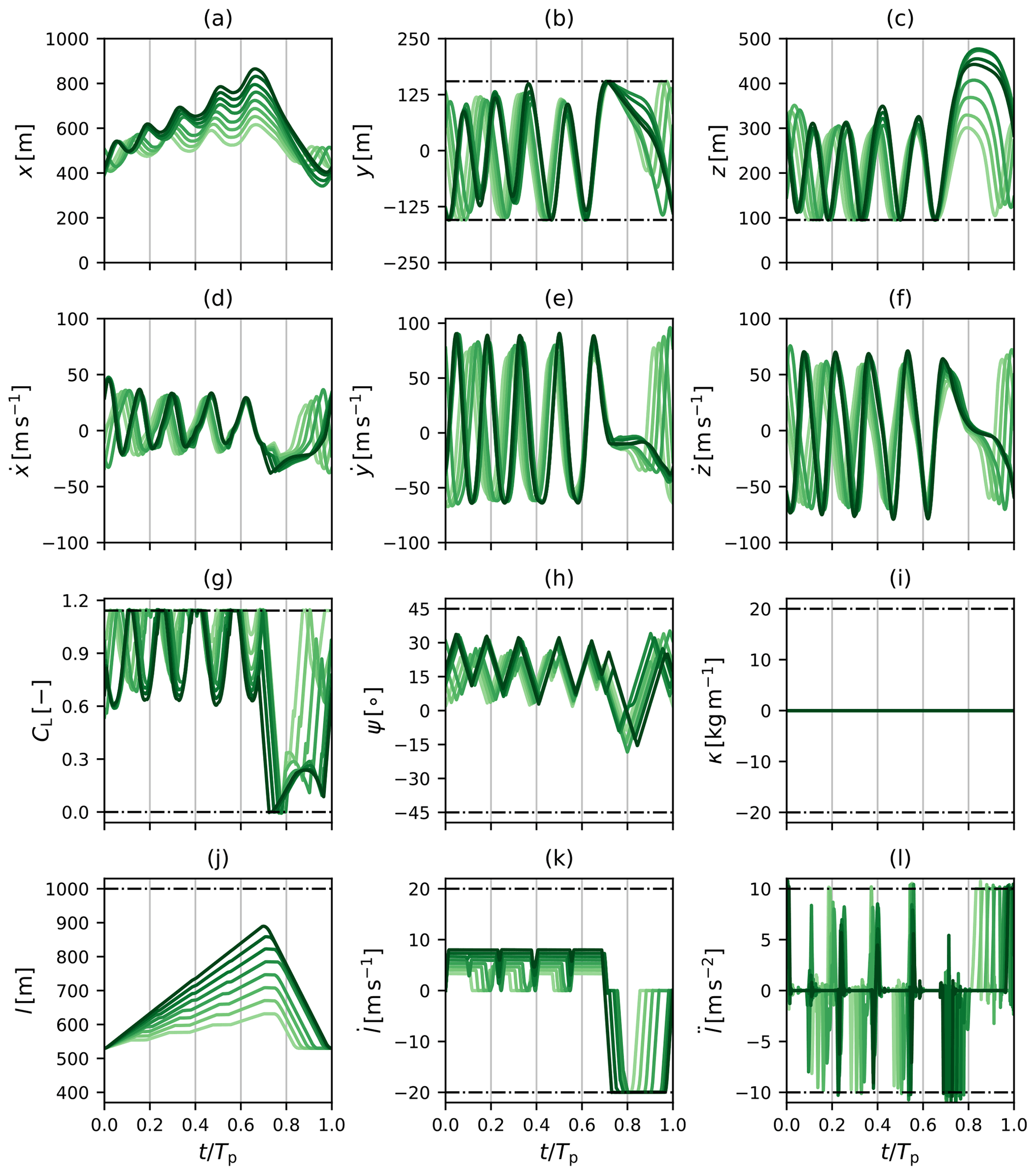
Figure B1Time series of the states normalised over one period Tp for the large-scale lift-mode AWE system (2) optimised for the wind speed range . The position q and velocity are respectively shown in the (a–b) and (d–f). The wing lift coefficient CL, roll angle Ψ, and on-board turbine thrust coefficient κ are shown in the (g–i). The tether variables l, , and , representing the length, speed, and acceleration of the tether, are shown in (j–l). The colour scheme is identical to Fig. 3, and the black dashed lines represent the eventual constraints applied to the variables in POCP (Eq. 33).
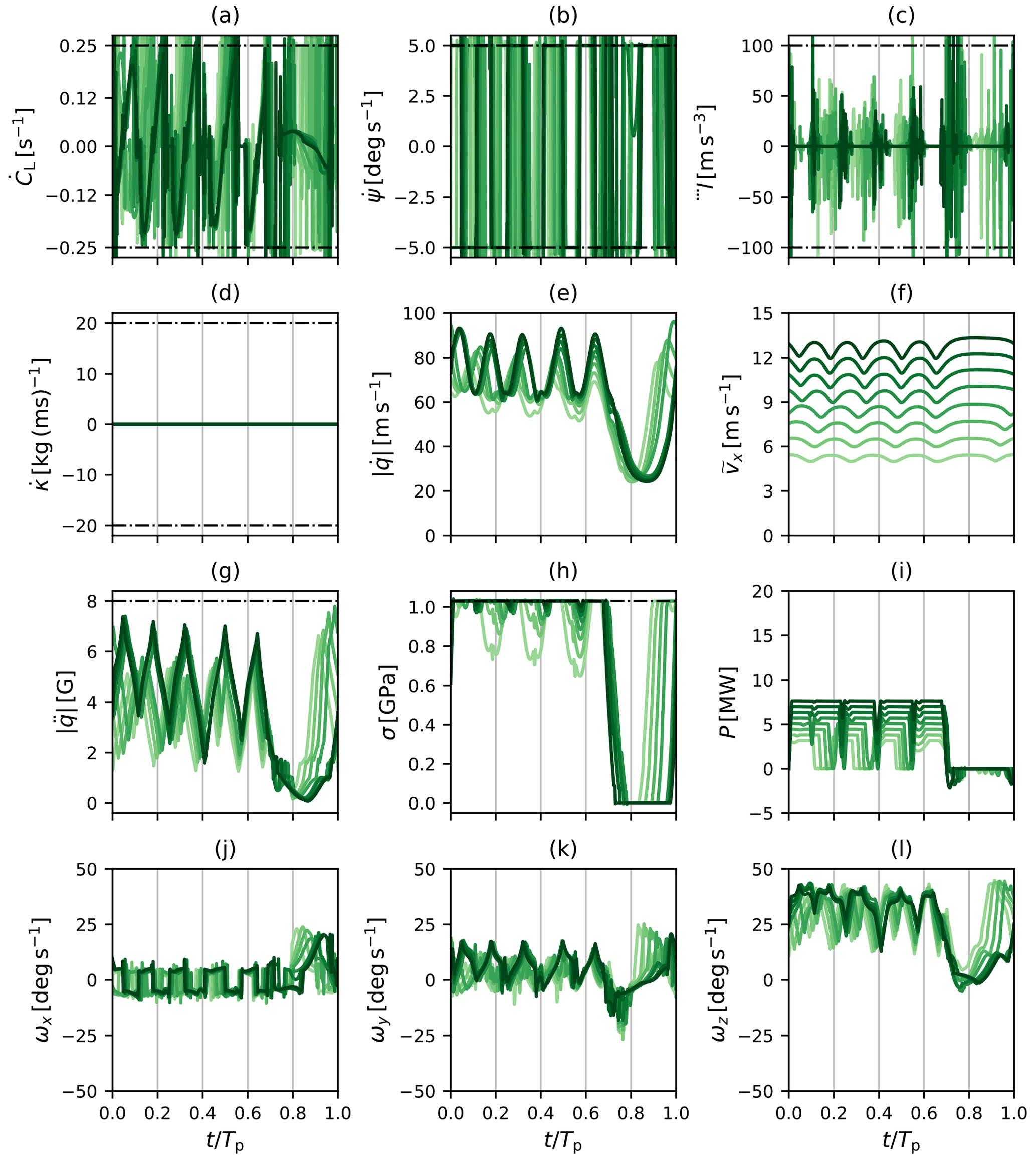
Figure B2Time series of the controls and additional quantities normalised over one period Tp for the large-scale lift-mode AWE system (2) optimised for the wind speed range . The control variables, i.e. the time derivatives of lift coefficient , roll angle , and thrust coefficient , and the tether jerk are shown in (a–d). The magnitude of the flight speed and the streamwise wind speed Ux are shown in (e) and (f). The magnitude of acceleration , the tether stress σ, and the instantaneous power P are shown in (h, i). The components of the angular velocity ω are shown in (j–l). The colour scheme is identical to Fig. 3, and the black dashed lines represent the eventual constraints applied to the variables in POCP (Eq. 33).
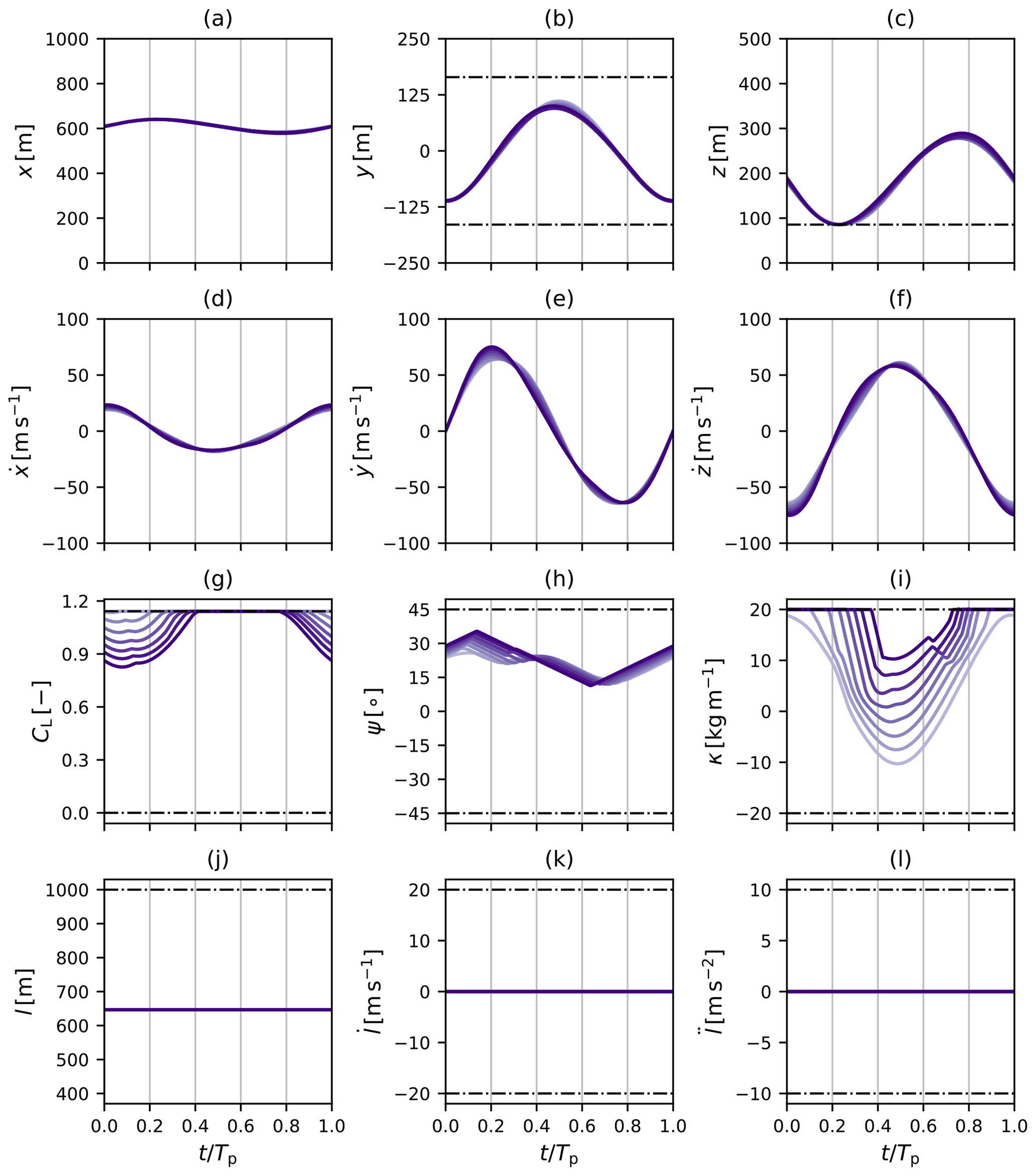
Figure B3Time series of the states normalised over one period Tp for the large-scale drag-mode AWE system optimised for the wind speed range . The position q and velocity are respectively shown in (a–c) and (d–f). The wing lift coefficient CL, roll angle Ψ, and on-board turbine thrust coefficient κ are shown in (g–i). The tether variables l, , and , representing the length, speed, and acceleration of the tether, are shown in (j–l). The colour scheme is identical to Fig. 3, and the black dashed lines represent the eventual constraints applied to the variables in POCP (Eq. 33).
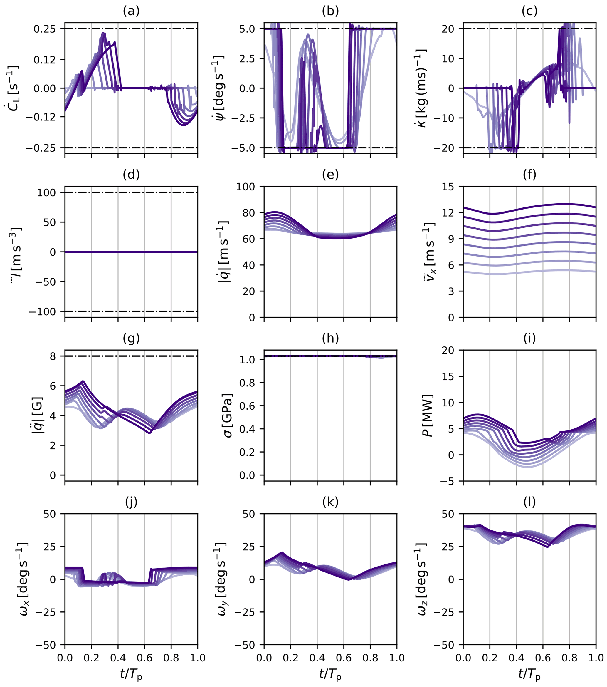
Figure B4Time series of the controls and additional quantities normalised over one period Tp for the large-scale drag-mode AWE system optimised for the wind speed range . The control variables, i.e. the time derivatives of lift coefficient , roll angle , and thrust coefficient , and the tether jerk are shown in (a–d). The magnitude of the flight speed and the streamwise wind speed Ux are shown in (e) and (f). The magnitude of acceleration , the tether stress σ, and the instantaneous power P are shown in (h, i). The components of the angular velocity ω are shown in (j–l). The colour scheme is identical to Fig. 3, and the black dashed lines represent the eventual constraints applied to the variables in POCP (Eq. 33).
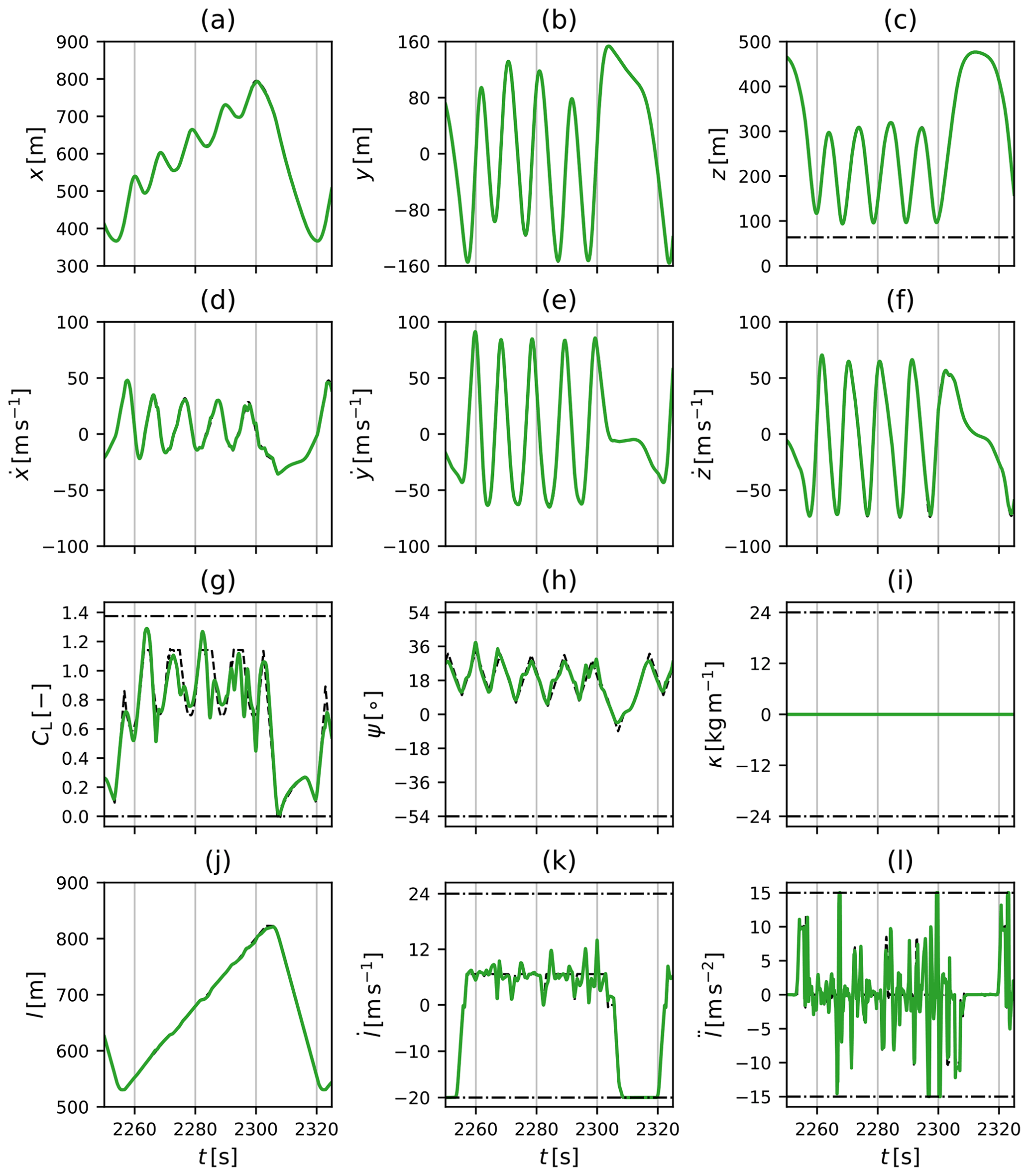
Figure B5Instantaneous states measured at the point mass of the lift-mode AWE system 003 (park L1) compared to their reference values. The position q and velocity are respectively shown in (a–c) and (d–f). The wing lift coefficient CL, roll angle Ψ, and on-board turbine thrust coefficient κ are shown in (g–i). The tether variables l, , and , representing the length, speed, and acceleration of the tether, are shown in (j–l). The black dashed and dashed–dotted lines respectively represent the variable references and the eventual constraints applied to the variables in NMPC (Eq. 36).
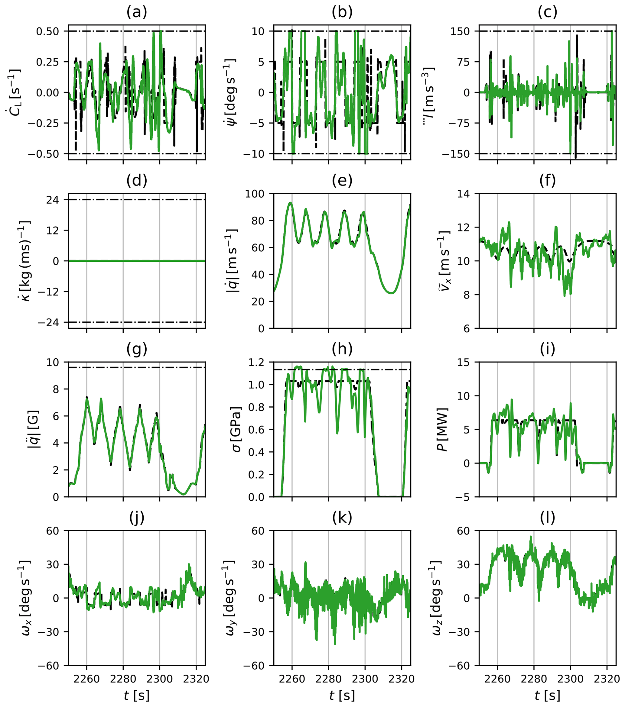
Figure B6Instantaneous controls and additional quantities measured at the point mass of the lift-mode AWE system 003 (park L1) compared to their reference values. The control variables, i.e. the time derivatives of lift coefficient , roll angle , and thrust coefficient , and the tether jerk are shown in (a–d). The magnitude of the flight speed and the streamwise wind speed are shown in (e) and (f). The magnitude of acceleration , the tether stress σ, and the instantaneous power P are respectively shown in (h, i). The components of the angular velocity ω are shown in (j–l). The black dashed and dashed–dotted lines respectively represent the variable references and the eventual constraints applied to the variables in NMPC (Eq. 36).
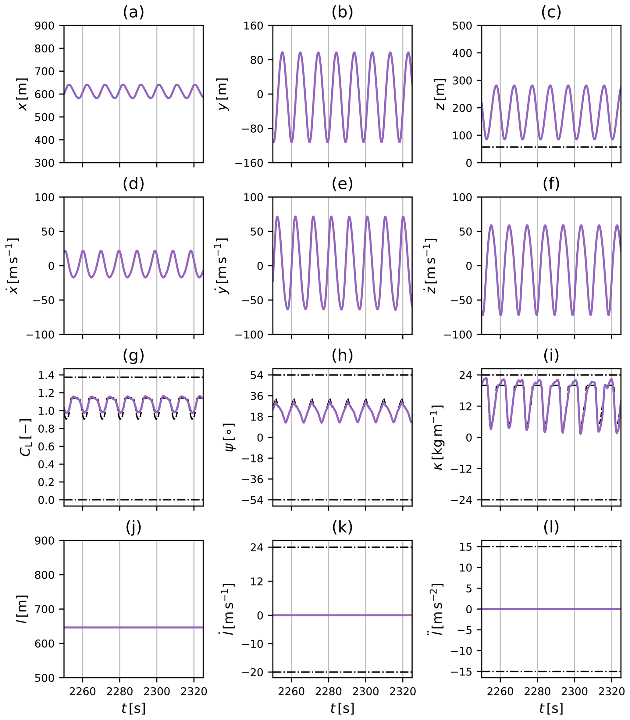
Figure B7Instantaneous states measured at the point mass of the drag-mode AWE system 003 (park D1) compared to their reference values. The position q and velocity are respectively shown in (a–c) and (d–f). The wing lift coefficient CL, roll angle Ψ, and on-board turbine thrust coefficient κ are shown in (g–i). The tether variables l, , and , representing the length, speed, and acceleration of the tether, are shown in (j–l). The black dashed and dashed–dotted lines respectively represent the variable references and the eventual constraints applied to the variables in NMPC (Eq. 36).

Figure B8Instantaneous controls and additional quantities measured at the point mass of the drag-mode AWE system 003 (park D1) compared to their reference values. The control variables, i.e. the time derivatives of lift coefficient , roll angle , and thrust coefficient , and the tether jerk are shown in (a–d). The magnitude of the flight speed and the streamwise wind speed are shown in (e) and (f). The magnitude of acceleration , the tether stress σ, and the instantaneous power P are respectively shown in (h, i). The components of the angular velocity ω are shown in (j–l). The black dashed and dashed–dotted lines respectively represent the variable references and the eventual constraints applied to the variables in NMPC (Eq. 36).
The SP-Wind flow solver is a proprietary software of KU Leuven while the toolbox awebox is openly accessible on GitHub (https://github.com/awebox, awebox, 2021). Time-resolved three-dimensional subsets of the ABL precursor simulations are openly accessible from the AWESCO Wind Field Datasets (https://doi.org/10.5281/zenodo.1418676) (Haas and Meyers, 2019). Virtual flight data of the AWE systems for the three AWES park configurations are presented in Appendix B and are openly accessible from the dataset “Large-eddy simulation of airborne wind energy farms: AWES virtual flight data” (https://doi.org/10.5281/zenodo.5705563) (Haas and Meyers, 2021).
TH and JM jointly set up the concept and objectives of the current work, partially based on a research collaboration plan previously devised by JM and MD. The PhD work of TH was supervised by JM and the PhD work of JDS by MD. TH performed code implementations in the LES code SP-Wind and carried out the AWES park simulations. TH generated the reference AWES trajectories using the awebox toolbox with support from JDS. JDS implemented the NMPC capability in the awebox toolbox and assisted TH for the coupling with SP-Wind. TH performed the data analysis and data visualisation. TH wrote the manuscript with major contributions from JM. JDS, JM, and MD revised the manuscript.
At least one of the (co-)authors is a member of the editorial board of Wind Energy Science. The peer-review process was guided by an independent editor, and the authors also have no other competing interests to declare.
Publisher's note: Copernicus Publications remains neutral with regard to jurisdictional claims in published maps and institutional affiliations.
The computational resources and services in this work were provided by the VSC (Flemish Supercomputer Center), funded by the Research Foundation Flanders (FWO) and the Flemish Government department EWI.
This research has been supported by the H2020 Marie Skłodowska-Curie Actions (grant nos. 642682 and 953348) and the Deutsche Forschungsgemeinschaft (grant nos. 277012063 and 424107692).
This paper was edited by Roland Schmehl and reviewed by two anonymous referees.
Alemi Ardakani, H. and Bridges, T. J.: Review of the 3-2-1 Euler Angles: a yaw–pitch–roll sequence, Tech. rep., http://personal.maths.surrey.ac.uk/T.Bridges/SLOSH/3-2-1-Eulerangles.pdf (last access: 19 May 2022), 2010. a
Allaerts, D. and Meyers, J.: Large eddy simulation of a large wind-turbine array in a conventionally neutral atmospheric boundary layer, Phys. Fluids, 27, 065108, https://doi.org/10.1063/1.4922339, 2015. a
Allaerts, D. and Meyers, J.: Boundary-layer development and gravity waves in conventionally neutral wind farms, J. Fluid Mech., 814, 95–130, 2017. a
Anderson, J. D.: Fundamentals of Aerodynamics, McGraw-Hill, ISBN 978-1-259-25134-4, 2010. a, b, c
Andersson, J. A. E., Gillis, J., Horn, G., Rawlings, J. B., and Diehl, M.: CasADi: a software framework for nonlinear optimization and optimal control, Mathematical Programming Computation, Springer, https://doi.org/10.1007/s12532-018-0139-4, 2018. a
Archer, C. L.: An Introduction to Meteorology for Airborne Wind Energy, in: Airborne Wind Energy, edited by: Ahrens, U., Diehl, M., and Schmehl, R., Springer-Verlag, Berlin, Heidelberg, 81–94, https://doi.org/10.1007/978-3-642-39965-7_5, 2013. a, b
Argatov, I. and Silvennoinen, R.: Efficiency of Traction Power Conversion Based on Crosswind Motion, in: Airborne Wind Energy, edited by: Ahrens, U., Diehl, M., and Schmehl, R., Springer-Verlag, Berlin, Heidelberg, 65–79, https://doi.org/10.1007/978-3-642-39965-7_4, 2013. a
awebox: awebox: Modelling and optimal control of single- and multiple-kite systems for airborne wind energy, GitHub [code], https://github.com/awebox (last access: 19 May 2022), 2021. a, b
Barthelmie, R. J., Pryor, S. C., Frandsen, S. T., Hansen, K. S., Schepers, J. G., Rados, K., Schlez, W., Neubert, A., Jensen, L. E., and Neckelmann, S.: Quantifying the Impact of Wind Turbine Wakes on Power Output at Offshore Wind Farms, J. Atmos. Ocean. Tech., 27, 1302–1317, https://doi.org/10.1175/2010JTECHA1398.1, 2010. a
Bauer, F., Kennel, R. M., Hackl, C. M., Campagnolo, F., Patt, M., and Schmehl, R.: Drag power kite with very high lift coefficient, Renew. Energy, 118, 290–305, https://doi.org/10.1016/j.renene.2017.10.073, 2018. a
Bulder, B., Bedon, G., and Bot, E.: Optimal wind farm power density analysis for future offshore wind farms, Tech. rep., http://resolver.tudelft.nl/uuid:dfe0ce2f-04fb-4db2-80db-52bc02cfb515 (last access: 19 May 2022), 2018. a
Calaf, M., Meneveau, C., and Meyers, J.: Large eddy simulation study of fully developed wind-turbine array boundary layers, Phys. Fluids, 22, 1–16, https://doi.org/10.1063/1.862466, 2010. a, b, c, d
Cherubini, A., Papini, A., Vertechy, R., and Fontana, M.: Airborne Wind Energy Systems: A review of the technologies, Renew. Sustain. Energ. Rev., 51, 1461–1476, https://doi.org/10.1016/j.rser.2015.07.053, 2015. a
De Lellis, M., Reginatto, R., Saraiva, R., and Trofino, A.: The Betz limit applied to Airborne Wind Energy, Renew. Energy, 127, 32–40, https://doi.org/10.1016/j.renene.2018.04.034, 2018. a
De Schutter, J., Bronnenmeyer, T., Paelinck, R., Diehl, M., and Leuthold, R.: Optimal control of stacked multi-kite systems for utility-scale airborne wind energy, in: 2019 IEEE 58th Conference on Decision and Control (CDC), https://doi.org/10.1109/CDC40024.2019.9030026, 2019. a, b
Diehl, M.: Airborne wind energy: Basic concepts and physical foundations, in: Airborne Wind Energy, edited by: Ahrens, U., Diehl, M., and Schmehl, R., Springer-Verlag, Berlin, Heidelberg, 3–22, https://doi.org/10.1007/978-3-642-39965-7_5, 2013. a, b
Dykes, K.: Optimization of Wind Farm Design for Objectives Beyond LCOE, vol. 1618, IOP Publishing, https://doi.org/10.1088/1742-6596/1618/4/042039, 2020. a
Echeverri, P., Fricke, T., Homsy, G., and Tucker, N.: The Energy Kite: Selected Results from the Design, Development, and Testing of Makani's Airborne Wind Turbines, Part I of III, Tech. rep., https://archive.org/details/theenergykite (last access: 19 May 2022), 2020. a, b
Gaunaa, M., Forsting, A. M., and Trevisi, F.: An engineering model for the induction of crosswind kite power systems, J. Phys.: Conf. Ser., 1618, 032010, https://doi.org/10.1088/1742-6596/1618/3/032010, 2020. a
Gohl, F. and Luchsinger, R. H.: Simulation Based Wing Design for Kite Power, in: Airborne Wind Energy, edited by: Ahrens, U., Diehl, M., and Schmehl, R., Springer-Verlag, Berlin, Heidelberg, 325–338, https://doi.org/10.1007/978-3-642-39965-7_5, 2013. a
Gros, S. and Diehl, M.: Modeling of airborne wind energy systems in natural coordinates, in: Airborne Wind Energy, edited by: Ahrens, U., Diehl, M., and Schmehl, R., Springer-Verlag, Berlin, Heidelberg, 181–203, https://doi.org/10.1007/978-3-642-39965-7_5, 2013. a, b, c
Gros, S. and Zanon, M.: Numerical Optimal Control With Periodicity Constraints in the Presence of Invariants, IEEE T. Automat. Control, 63, 2818–2832, https://doi.org/10.1109/TAC.2017.2772039, 2018. a
Gros, S., Zanon, M., and Diehl, M.: Control of Airborne Wind Energy systems based on Nonlinear Model Predictive Control and Moving Horizon Estimation, in: 2013 European Control Conference (ECC), 1017–1022, https://doi.org/10.23919/ECC.2013.6669713, 2013. a
Haas, T. and Meyers, J.: Comparison study between wind turbine and power kite wakes, J. Phys.: Conf. Ser., 854, 012019, https://doi.org/10.1088/1742-6596/854/1/012019, 2017. a, b
Haas, T. and Meyers, J.: AWESCO Wind Field Datasets, Zenodo [data set], https://doi.org/10.5281/zenodo.1418676, 2019. a, b
Haas, T. and Meyers, J.: Large-eddy simulation of airborne wind energy farms: AWES virtual flight data, Zenodo [data set], https://doi.org/10.5281/zenodo.5705563, 2021. a
Haas, T., De Schutter, J., Diehl, M., and Meyers, J.: Wake characteristics of pumping mode airborne wind energy systems, J. Phys.: Conf. Ser., 1256, 012016, https://doi.org/10.1088/1742-6596/1256/1/012016, 2019b. a
Horn, G., Gros, S., and Diehl, M.: Numerical trajectory optimization for airborne wind energy systems described by high fidelity aircraft models, in: Airborne Wind Energy, edited by: Ahrens, U., Diehl, M., and Schmehl, R., Springer-Verlag, Berlin, Heidelberg, 205–218, https://doi.org/10.1007/978-3-642-39965-7_5, 2013. a
Houska, B. and Diehl, M.: Optimal control for power generating kites, in: 2007 European Control Conference (ECC), 3560–3567, https://doi.org/10.23919/ECC.2007.7068861, 2007. a
HSL: A collection of Fortran codes for large scale scientific computation, http://www.hsl.rl.ac.uk (last access: 19 May 2022), 2011. a
Jenkins, N., Burton, A., Sharpe, D., and Bossanyi, E.: Wind Energy Handbook, Wiley, ISBN 978-1-119-99272-1, 2001. a, b
Jeong, J. and Hussain, F.: On the identification of a vortex, J. Fluid Mech., 285, 69–94, https://doi.org/10.1017/S0022112095000462, 1995. a
Jimenez, A., Crespo, A., Migoya, E., and Garcia, J.: Advances in large-eddy simulation of a wind turbine wake, J. Phys.: Conf. Ser., 75, 012041, https://doi.org/10.1088/1742-6596/75/1/012041, 2007. a
Kaufman-Martin, S., Naclerio, N., May, P., and Luzzatto-Fegiz, P.: An entrainment-based model for annular wakes, with applications to airborne wind energy, Wind Energy, 25, 419–431, https://doi.org/10.1002/we.2679, 2022. a
Kheiri, M., Bourgault, F., Saberi Nasrabad, V., and Victor, S.: On the aerodynamic performance of crosswind kite power systems, J. Wind Eng. Indust. Aerodyn., 181, 1–13, https://doi.org/10.1016/j.jweia.2018.08.006, 2018. a, b
Kruijff, M. and Ruiterkamp, R.: A Roadmap Towards Airborne Wind Energy in the Utility Sector, in: Airborne Wind Energy: Advances in Technology Development and Research, edited by: Schmehl, R., Springer Singapore, 643–662, https://doi.org/10.1007/978-981-10-1947-0, 2018. a, b, c, d, e, f
Leuthold, R., Gros, S., and Diehl, M.: Induction in Optimal Control of Multiple-Kite Airborne Wind Energy Systems, in: Proceedings of 20th IFAC World Congress, Toulouse, France, https://doi.org/10.1016/j.ifacol.2017.08.026, 2017. a, b
Leuthold, R., De Schutter, J., Malz, E., Licitra, G., Gros, S., and Diehl, M.: Operational Regions of a Multi-Kite AWE System, in: 2018 European Control Conference (ECC), 52–57, https://doi.org/10.23919/ECC.2018.8550199, 2018. a
Leuthold, R., Crawford, C., Gros, S., and Diehl, M.: Engineering Wake Induction Model For Axisymmetric Multi-Kite Systems, J. Phys.: Conf. Ser., 1256, 012009, https://doi.org/10.1088/1742-6596/1256/1/012009, 2019. a
Licitra, G., Sieberling, S., Engelen, S., Williams, P., Ruiterkamp, R., and Diehl, M.: Optimal control for minimizing power consumption during holding patterns for airborne wind energy pumping system, in: 2016 European Control Conference (ECC), 1574–1579, https://doi.org/10.1109/ECC.2016.7810515, 2016. a
Licitra, G., Williams, P., Gillis, J., Ghandchi, S., Sieberling, S., Ruiterkamp, R., and Diehl, M.: Aerodynamic Parameter Identification for an Airborne Wind Energy Pumping System, in: 20th IFAC World Congress, IFAC-PapersOnLine, 50, 11951–11958, https://doi.org/10.1016/j.ifacol.2017.08.1038, 2017. a
Licitra, G., Koenemann, J., Bürger, A., Williams, P., Ruiterkamp, R., and Diehl, M.: Performance assessment of a rigid wing Airborne Wind Energy pumping system, Energy, 173, 569–585, https://doi.org/10.1016/j.energy.2019.02.064, 2019. a
Loyd, M. L.: Crosswind Kite Power, J. Energy, 4, 106–111, https://doi.org/10.2514/3.48021, 1980. a
Makani Power: Response to the federal aviation authority, Tech. rep., Makani Power, http://www.energykitesystems.net/FAA/FAAfromMakani.pdf (last access: 19 May 2022), 2012. a, b, c, d
Malz, E., Zanon, M., and Gros, S.: A Quantification of the Performance Loss of Power Averaging in Airborne Wind Energy Farms, in: 2018 European Control Conference (ECC), https://doi.org/10.23919/ECC.2018.8550357, 2018. a
Malz, E., Koenemann, J., Sieberling, S., and Gros, S.: A reference model for airborne wind energy systems for optimization and control, Renew. Energy, 140, 1004–1011, https://doi.org/10.1016/j.renene.2019.03.111, 2019. a, b, c, d
Martinez-Tossas, L. A., Churchfield, M. J., Yilmaz, A. E., Sarlak, H., Johnson, P. L., Sorensen, J. N., Meyers, J., and Meneveau, C.: Comparison of four large-eddy simulation research codes and effects of model coefficient and inflow turbulence in actuator-line-based wind turbine modeling, J. Renew. Sustain. Energ., 10, 033301, https://doi.org/10.1063/1.5004710, 2018. a
Mason, P. J. and Thomson, D. J.: Stochastic backscatter in large-eddy simulations of boundary layers, J. Fluid Mechan., 242, 51–78, https://doi.org/10.1017/S0022112092002271, 1992. a
Munters, W., Meneveau, C., and Meyers, J.: Turbulent Inflow Precursor Method with Time-Varying Direction for Large-Eddy Simulations and Applications to Wind Farms, Bound.-Lay. Meteorol., 159, 305–328, https://doi.org/10.1007/s10546-016-0127-z, 2016. a, b
Pope, S. B.: Turbulent Flows, Cambridge University Press, https://doi.org/10.1017/CBO9780511840531, 2000. a
Porte-Agel, F., Bastankhah, M., and Shamsoddin, S.: Wind-turbine and wind-farm flows: a review, Bound.-Lay. Meteorol., 174, 1–59, 2020. a
Rapp, S., Schmehl, R., Oland, E., and Haas, T.: Cascaded Pumping Cycle Control for Rigid Wing Airborne Wind Energy Systems, J. Guidance Control Dynam., 42, 2456–2473, https://doi.org/10.2514/1.G004246, 2019. a
Read, R.: Kite Networks for HarvestingWind Energy, in: Airborne Wind Energy: Advances in Technology Development and Research, edited by: Schmehl, R., Springer, Singapore, 515–517, https://doi.org/10.1007/978-981-10-1947-0, 2018. a
Roque, L. A., Paiva, L. T., Fernandes, M. C., Fontes, D. B., and Fontes, F. A.: Layout optimization of an airborne wind energy farm for maximum power generation, in: the 6th International Conference on Energy and Environment Research – Energy and environment: challenges towards circular economy, Energy Rep., 6, 165–171, https://doi.org/10.1016/j.egyr.2019.08.037, 2020. a
Schelbergen, M. and Schmehl, R.: Validation of the quasi-steady performance model for pumping airborne wind energy systems, J. Phys.: Conf. Ser., 1618, 32003, https://doi.org/10.1088/1742-6596/1618/3/032003, 2020. a
Sorensen, J. N. and Shen, W. Z.: Numerical Modeling of Wind Turbine Wakes, J. Fluids Eng., 124, 393, https://doi.org/10.1115/1.1471361, 2002. a
Sternberg, J., Goit, J., Gros, S., Meyers, J., and Diehl, M.: Robust and stable periodic flight of power generating kite systems in a turbulent wind flow field, IFAC Proceedings Volumes (IFAC-PapersOnline), 45, 140–145, https://doi.org/10.3182/20120913-4-IT-4027.00009, 2012. a
Stevens, R. J. and Meneveau, C.: Flow Structure and Turbulence in Wind Farms, Annu. Rev. Fluid Mech., 49, 311–339, https://doi.org/10.1146/annurev-fluid-010816-060206, 2017. a
Storey, R. C., Norris, S. E., and Cater, J. E.: An actuator sector method for efficient transient wind turbine simulation, Wind Energy, 18, 699–711, https://doi.org/10.1002/we.1722, 2015. a, b
Trevisi, F., Gaunaa, M., and Mcwilliam, M.: The Influence of Tether Sag on Airborne Wind Energy Generation, J. Phys.: Conf. Ser., 1618, 032006, https://doi.org/10.1088/1742-6596/1618/3/032006, 2020. a
Troen, I. and Lundtang Petersen, E.: European Wind Atlas, Tech. rep., Risø National Laboratory, ISBN 87-550-1482-8, 1989. a
Troldborg, N., Sorensen, J. N., and Mikkelsen, R.: Numerical simulations of wake characteristics of a wind turbine in uniform inflow, Wind Energy, 13, 86–99, https://doi.org/10.1002/we.345, 2010. a, b, c
Vitsas, A. and Meyers, J.: Multiscale aeroelastic simulations of large wind farms in the atmospheric boundary layer, J. Phys.: Conf. Ser., 753, 082020, https://doi.org/10.1088/1742-6596/753/8/082020, 2016. a
Wächter, A.: An Interior Point Algorithm for Large-Scale Nonlinear Optimization with Applications in Process Engineering, PhD thesis, Carnegie Mellon University, http://users.iems.northwestern.edu/~andreasw/pubs/waechter_thesis.pdf (last access: 19 May 2022), 2002. a
XFLR5: XFLR5: XFLR5 is an analysis tool for airfoils, wings and
planes, https://sourceforge.net/projects/xflr5/ (last access: 19 May 2022), 2021. a
XFOIL: XFOIL: Subsonic Airfoil Development System,
https://web.mit.edu/drela/Public/web/xfoil/ (last access: 19 May 2022), 2021. a
Zanon, M.: Efficient Nonlinear Model Predictive Control Formulations for Economic Objectives with Aerospace and Automotive Applications, https://limo.libis.be/primo-explore/fulldisplay?docid=LIRIAS1693005&context=L&vid=Lirias&search_scope=Lirias&tab=default_tab&fromSitemap=1 (last access: 19 May 2022), 2015. a
Zanon, M., Gros, S., Andersson, J., and Diehl, M.: Airborne Wind Energy Based on Dual Airfoils, IEEE T. Control Syst. Technol., 21, 1215–1222, https://doi.org/10.1109/TCST.2013.2257781, 2013a. a
Zanon, M., Gros, S., and Diehl, M.: Model predictive control of rigid-airfoil airborne wind energy systems, in: Airborne Wind Energy, edited by: Ahrens, U., Diehl, M., and Schmehl, R., Springer-Verlag, Berlin, Heidelberg, 219–234, https://doi.org/10.1007/978-3-642-39965-7_5, 2013b. a, b, c
- Abstract
- Introduction
- Methodology
- Simulation setup
- AWE farm simulation and results
- Conclusions
- Appendix A: Investigation of single-AWES wake characteristics
- Appendix B: Data accessibility
- Code and data availability
- Author contributions
- Competing interests
- Disclaimer
- Acknowledgements
- Financial support
- Review statement
- References