Impact of the wind field at the complex-terrain site Perdigão on the surface pressure fluctuations of a wind turbine

The surface pressure fluctuations, which are a source of low-frequency noise emissions, are numerically investigated on a 2 MW wind turbine under different inflow conditions. In order to evaluate the impact of a complex-terrain flow, a computational setup is presented that is aimed at reproducing a realistic flow field in the complex terrain in Perdigão, Portugal. A precursor simulation with the steady-state atmospheric computational fluid dynamics (CFD) code E-Wind is used, which was calibrated with meteorological (met) mast data to generate a site- and situation-specific inflow for a high-resolution delayed detached-eddy simulation (DDES) with FLOWer. A validation with lidar and met mast data reveals a good agreement of the flow field in the vicinity of the turbine in terms of mean wind speed and wind direction, whereas the turbulence intensity is slightly underestimated. Further downstream in the valley and on the second ridge, the deviations between simulation and measurement become significantly larger. The geometrically resolved turbine is coupled to the structural solver SIMPACK and simulated both in the complex terrain and in flat terrain with simpler inflows as reference. The surface pressure fluctuations are evaluated on the tower and blades. It is found that the periodic pressure fluctuations at the tower sides and back are dominated by vortex shedding, which strongly depends on the inflow and is reduced by inflow turbulence. However, the dominant pressure fluctuations on the upper part of the tower, which are caused by the blade–tower interaction, remain almost unchanged by the different inflows. The predominant pressure fluctuations on the blades occur with the rotation frequency. They are caused by a combination of rotor tilt, vertical wind shear and inclined flow and are thus strongly dependent on the inflow and the surrounding terrain. The inflow turbulence masks fluctuations at higher harmonics of the blade–tower interaction with its broadband characteristic caused by the interaction of the leading edge and the inflow turbulence.

1 Introduction

In the course of the onshore expansion of wind energy, more and more wind turbines (WTs) are being erected in complex terrain. The disturbances of the inflow angle, the strong turbulence and the inhomogeneity of the wind field pose a challenge for the prediction of turbine loads, performance and noise emission. Especially the low-frequency acoustic emissions are controversially discussed in the context of public acceptance of WTs in onshore wind parks. The basis for an accurate prediction of acoustic low-frequency emissions is the correct simulation and understanding of their aerodynamic source, namely the surface pressure fluctuations on the tower and blades (Yauwenas, 2017; Klein, 2019). These are caused by the blade–tower interaction, the inflow turbulence and the vortex shedding, all of which are affected by the surrounding terrain and its specific flow field. The increase in computational resources enables high-fidelity simulations to capture more and more of these aerodynamic interactions in a complex-terrain site and to evaluate the corresponding phenomena.

1.1 Numerical approaches for complex terrain and wind turbine simulations

Reliable methods for predicting flow characteristics are of great importance for profound site assessment, especially in complex terrain. Flow over hills is accelerated and can cause recirculation regions, and turbulence characteristics are altered, all of which have been studied in research for decades, as the overview of Belcher and Hunt (1998) shows. These effects hold positive potential in terms of wind turbine performance but also bear risks. In industry, computationally cheap approaches, such as steady-state Reynolds-averaged Navier–Stokes (RANS) simulations (Alletto et al., 2018), are used for assessing risky turbine positions in complex terrain. Large-scale and long-term meteorological effects can be captured with the Weather Research and Forecasting (WRF) model, which allows the nesting of large-eddy simulations (LESs) at the expense of only coarsely resolved topographic terrain features, such as in Wagner et al. (2019). To capture the unsteady effects occurring in the atmospheric boundary layer (ABL) and their interaction with complex terrain, unsteady RANS (URANS) simulations, as in Koblitz (2013), can be used. If the focus is on resolving the ABL or on the aerodynamic interaction of the inflow and the turbine, hybrid RANS–LES models are necessary, since the small-scale vortices must be resolved. Bechmann and Sørensen (2010) simulated the flow over a hill with a hybrid formulation similar to the detached-eddy simulation (DES) with good results, especially for the turbulence level. Schulz et al. (2016) conducted delayed detached-eddy simulations (DDESs) to evaluate the effect of complex terrain on the performance of a WT, and the general suitability of DDES for detailed investigations of wind turbine aerodynamics is demonstrated by Weihing et al. (2018). Sørensen and Schreck (2014) performed DDES and URANS simulations of the NREL Phase-VI rotor and found that although DDES does not improve the quality of the mean power prediction, it significantly increases the accuracy of the predicted load spectra compared to URANS. For the overall objective of the present paper, the investigation of surface pressure fluctuations under complex inflow conditions, it is therefore highly advisable to use DDES.

1.2 The complex-terrain site Perdigão

A widely studied complex-terrain site in the field of wind energy is the double ridge in Perdigão in central Portugal. The site consists of two parallel, well-exposed ridges, each overlooking the surrounding area by about 300 m. A single WT is located on the southwestern ridge. A detailed description of the orography and vegetation at the site can be found in Vasiljević et al. (2017). During the 2017 field campaign in Perdigão, a comprehensive set of measurement data of the flow over the complex terrain and of the behaviour of the WT were collected. The measurement equipment includes meteorological (met) masts, lidars and microphones (Fernando et al., 2019). This campaign is part of the New European Wind Atlas (NEWA) (Mann et al., 2017) funded by the European Union, which provides maps of wind statistics in complex terrains that can be used as a benchmark for site assessment. In order to obtain accurate simulation results, the terrain model on which the computational fluid dynamics (CFD) simulations are based must be correspondingly detailed. Therefore, Palma et al. (2020) created a detailed digital terrain model (DTM) with a resolution of 2 m, which includes orography and vegetation.

In many studies, simulations of the flow field in Perdigão have already been carried out to investigate the effects of orography, vegetation, thermal stratification and meteorological effects in general. Wagner et al. (2019) performed nested WRF-LES for the Iberian Peninsula with a highest resolution of 200 m around Perdigão covering almost 50 d. They showed that the southwest wind during the day experiences a clockwise turning and that the frequent nocturnal low-level jets over the double ridge from the northeast already develop in Spain. Coupled WRF and URANS simulations were used by Olsen (2018) to include changing weather patterns as well as local orographic and surface effects. Characteristic eddy structures behind the ridges were observed, and with a finest mesh resolution of 80 m the mean wind speed was captured well. Steady-state RANS calculations were used by Palma et al. (2020) to discuss the impact of the resolution of the terrain model as well as of the CFD mesh on the local flow. They found that the flow in the valley was most affected by the resolution and recommend a resolution below 40 m. Salim Dar et al. (2019) performed LES of the double ridge in Perdigão with a resolution of 10 m including the WT, represented with an actuator-disc model. They investigated the wake behaviour and found that the shape of the velocity deficit profile is preserved in the downstream direction even in complex terrain, which is known as self-similarity. In addition, they found that the streamwise velocity at hub height varies with the change in terrain characteristics caused by a change in resolution. Simulations of the interaction between turbulent terrain flow and local wind turbine aerodynamics using a fully resolved turbine in Perdigão have not been published to the authors' knowledge.

1.3 Scope and objectives

The aim of the present paper is to numerically investigate the influence of the flow in the complex terrain in Perdigão on the unsteady pressure distributions on the turbine surface, which are a source of low-frequency noise emissions. For this purpose, a fluid–structure-coupled DDES of the fully resolved 2 MW wind turbine in the complex terrain of Perdigão including forest and turbulent inflow is conducted with the CFD solver FLOWer. A measured flow situation is reproduced by using data from a precursor simulation with the atmospheric CFD code E-Wind, which was calibrated with met mast data, as inflow for FLOWer. In a first step, the simulated terrain flow (without the turbine) is validated by a comparison with measurements in Perdigão to prove the quality and suitability of the process chain for the detailed simulation of the wind field in the complex terrain. Then, the WT is included in the fluid–structure-coupled FLOWer simulation, and the turbine wake, the global loads and the deformations are checked for plausibility. Finally, the unsteady pressure distributions on the tower and blades are investigated in detail, focusing on the influence of the inflow on the interaction between blades and tower as well as on the vortex shedding at the tower. The observations are compared with the results of DDES of the same turbine in flat terrain with both uniform and turbulent inflow to highlight peculiarities.

2 Numerical tools

The high-fidelity process chain for the calculation of unsteady aerodynamics under site- and situation-specific inflow in complex terrain comprises several solvers. The atmospheric steady-state CFD RANS solver E-Wind is used for the simulation of the Perdigão site and provides the inflow conditions for the unsteady high-resolution DDES with the CFD solver FLOWer of the near field around the turbine. The geometrically resolved turbine can be included in this simulation, and a time-accurate coupling to the structural solver SIMPACK enables the consideration of aeroelastic effects caused by the fluid–structure interaction (FSI).

2.1 Atmospheric CFD code – E-Wind

E-Wind is an atmospheric CFD tool developed and used by Enercon for wind resource assessment (Alletto et al., 2018). E-Wind solves the steady-state RANS equations using the k–ε turbulence model, where the turbulent kinetic energy k and the rate of dissipation ε are the two transported variables. The governing equations are adapted to ABL conditions, e.g. complex terrain, roughness and forest (vegetation), atmospheric stability, and the Coriolis force (Sogachev et al., 2012), and solved using the open-source code OpenFOAM (v1712) as the core solver within E-Wind. Since the exact boundary condition (BC) for ground roughness and thermal stability are often unknown, a scaling of the roughness map and the ground heat flux can be used in a calibration process against mast measurements to match the vertical wind shear at the met mast location. For a detailed description of the calibration process see Adib et al. (2021).

2.2 Unsteady CFD solver – FLOWer

The basis for the numerical simulations of the WT is the CFD solver FLOWer, which was originally developed by the German Aerospace Center (DLR) (Kroll et al., 2000). It is a compressible, block-structured RANS solver. The numerical scheme is based on a finite-volume formulation. The Chimera technique implemented allows the use of independent grids for the individual components of the WT and the background. The solver has been continuously extended at the Institute of Aerodynamics and Gas Dynamics (IAG) to improve its suitability for wind turbine simulations. Among others, the fifth-order weighted essentially non-oscillatory scheme WENO is available for spatial discretization (Kowarsch et al., 2013), and several hybrid RANS–LES schemes have been implemented in FLOWer (Weihing et al., 2018). Furthermore, a body force approach is included to superimpose atmospheric turbulence on the inflow (Schulz et al., 2016) and forest regions are accounted for by volume forces added to the momentum equation of the Navier–Stokes equations (Letzgus et al., 2018). The work of Klein et al. (2018) introduced a revised coupling to the multi-body simulation tool SIMPACK.

2.3 Structural solver – SIMPACK

SIMPACK is commercial software for the simulation of multi-body systems. The dynamic systems can consist of rigid and flexible bodies connected by joint elements. The flexible turbine components such as the tower and blades can be modelled either as beams or as modal bodies by reading in the modal properties. External forces such as aerodynamic forces can be defined internally or imported from other programs via a predefined interface environment. Controllers can also be integrated. SIMPACK has recently been used by industrial and research groups for the simulation of WTs, e.g. Luhmann et al. (2017) and Guma et al. (2021).

3 Computational setup

The setup of the complex-terrain simulation aims to reproduce a measured flow situation to allow for a validation of the local wind field simulated with FLOWer. The situation is selected based on operating data from the turbine in Perdigão, with the objective of having fairly constant operating conditions close to the rated conditions. This is found to be the case for a 30 min interval on 10 May 2017 from 15:15:00 UTC with an inflow from the southwest (230^∘). The measured data are averaged over this interval before serving as a reference.

3.1 Atmospheric precursor simulation with E-Wind

E-Wind is used to extrapolate a site- and situation-specific mean flow field from the measured wind profile at a met mast location. This provides a prediction of the flow conditions at any other location at the site, including the position where the FLOWer domain inlet is placed and where no measurement data are available. Thus, the necessary FLOWer inflow conditions can be extracted from the modelled flow field. Due to the high resolution and up-to-date terrain and forest maps, no roughness calibration is performed. For the selected situation, good calibration results can be obtained for met mast 20 under neutral thermal conditions (no ground heat flux). The equations in E-Wind are discretized using a mixed first-order–second-order scheme (Alletto et al., 2018). The convergence criteria of the simulation for the velocity and k are reached after about 2200 iterations.

3.1.1 Mesh and boundary conditions for E-Wind

E-Wind uses a cylindrical domain with a diameter of 22.5 km and a height of 6 km (see Fig. 1). The Perdigão terrain mesh in E-Wind is based on the high-resolution (2 m) map provided by Palma et al. (2020). It is resampled to a resolution of 10 m to fit the mesh resolution and to avoid artefacts in the mesh. Since the scanned area is smaller than the computational domain, the map is extended with data from the Shuttle Radar Topography Mission (SRTM). The coordinate system used for both the maps and the domain is ETRS89 / Portugal TM06 (EPSG:3763). To allow for homogeneous inflow, the terrain is flattened towards the lateral boundaries by a 3 km wide ramp followed by a 2 km wide flat area.

Figure 1 Mesh of E-Wind for a wind direction of 230^∘ (inflow parallel to cutting plane).

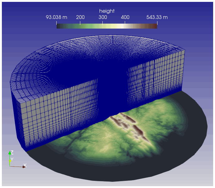
The structured mesh for E-Wind has about 9.4 million cells. A fine grid with 10 m horizontal resolution and 1 m vertical resolution is used in the centre of the domain, which is coarsened towards the lateral and upper boundaries. At a height of 500 m above the highest terrain elevation, the horizontal resolution is doubled to 20 m. The mesh is aligned with the wind direction (WD) at the hub height of WD_hub=230^∘. The ground surface is modelled as no-slip wall, using wall functions for the turbulent quantities and a fixed heat flux for the temperature. For the upper boundary, slip conditions for velocity, temperature, k and ε are applied, and the pressure gradient is fixed to prescribe the geostrophic forcing. At the sides of the domain, an inletOutlet OpenFOAM BC is used with a precomputed profile for the inflow and a zero gradient condition for the outflow. For more details, see Alletto et al. (2018). The geostrophic wind speed is set to 11 m s⁻¹ and the geostrophic wind direction to 242^∘.

3.1.2 Vegetation in E-Wind

To account for vegetation in E-Wind, a map of the roughness length z₀ must be provided, which is then applied as either roughness or forest depending on the actual z₀ value. The provided forest height map with 2 m resolution (Palma et al., 2020) is also resampled to 10 m and smoothed with a Gaussian filter. The forest height is divided by the forest scaling factor FSF=10 to derive the z₀ map. The calculated z₀ values are then classified into eight different classes. The forest model described in Alletto et al. (2018) is applied for z₀>0.5 m, which applies to the three highest z₀ classes. The constant leaf area density LAD=0.2, the drag coefficient c_d=0.15 and the forest height $h=\mathrm{FSF}\cdot z_{\mathrm{0}}$ are used. The five lower classes are treated as roughness with a wall function (OpenFOAM BC nutkAtmRoughWallFunction). A constant value of z₀=1.0 m is used outside of the provided map, representing forest with h=10 m.

3.2 Unsteady simulation of terrain flow with FLOWer

The high-resolution unsteady simulations with FLOWer are carried out as DDES (Spalart et al., 2006) based on the Menter shear stress transport (SST) k–ω RANS model (Gritskevich et al., 2013), following the literature mentioned in Sect. 1.1 (Schulz et al., 2016; Weihing et al., 2018; Sørensen and Schreck, 2014). The flow is considered to be fully turbulent. An implicit second-order dual-time-stepping scheme is deployed for time integration. The second-order Jameson–Schmidt–Turkel (JST) scheme is used for the spatial discretization in the boundary layer (BL) cells, and the fifth-order WENO scheme is applied to the Perdigão terrain mesh to reduce the dissipation of vortices. A physical time step corresponding to $\mathrm{\Delta }t\approx \mathrm{0.5}{\mathrm{\Delta }}_{\mathrm{0}}/u_{\mathrm{hub}}=\mathrm{0.05}$ s is used, where Δ₀ is the smallest grid size and u_hub is the horizontal flow velocity at the turbine position at hub height from E-Wind. The dual-time-stepping scheme uses 80 inner iterations, which decreases the global root-mean-square density residual by 2 orders of magnitude. The simulation is run for 300 s to propagate the injected turbulence through the domain and develop the mean velocity field before the evaluation can begin.

3.2.1 Terrain mesh and boundary conditions for FLOWer

The basis of the Perdigão terrain mesh for FLOWer is the same highly resolved (2 m resolution) DTM of the site in Perdigão (Palma et al., 2020) as for E-Wind (without resampling). This DTM is shifted so that the tower base of the turbine is located at $x=y=\mathrm{0}$ and rotated to align the x axis with WD_hub=230^∘. To reduce the impact of the domain boundaries on the flow field in the region of interest, they are placed far away (−768 m $<x<$ 3072 m, −3072 m $<y<$ 3072 m), as visualized in Fig. 2. In addition, the DTM is smoothed at the lateral and rear boundaries (dark blue area) to blend into a flat bottom (light blue area), while it remains unchanged in the region of interest (grey area). This allows periodic BCs to be used laterally, and, due to the associated reduced flow gradients, problems with numerical stability can be avoided. The domain inlet is placed at the base of the first ridge and is carried out as a Dirichlet BC. The domain extends vertically up to z=3447 m. The simulated area above the ground is thus about 10 times the maximum height difference of the terrain, which allows for a symmetry BC at the top (Koblitz, 2013). A zero-order extrapolation is applied at the outlet.

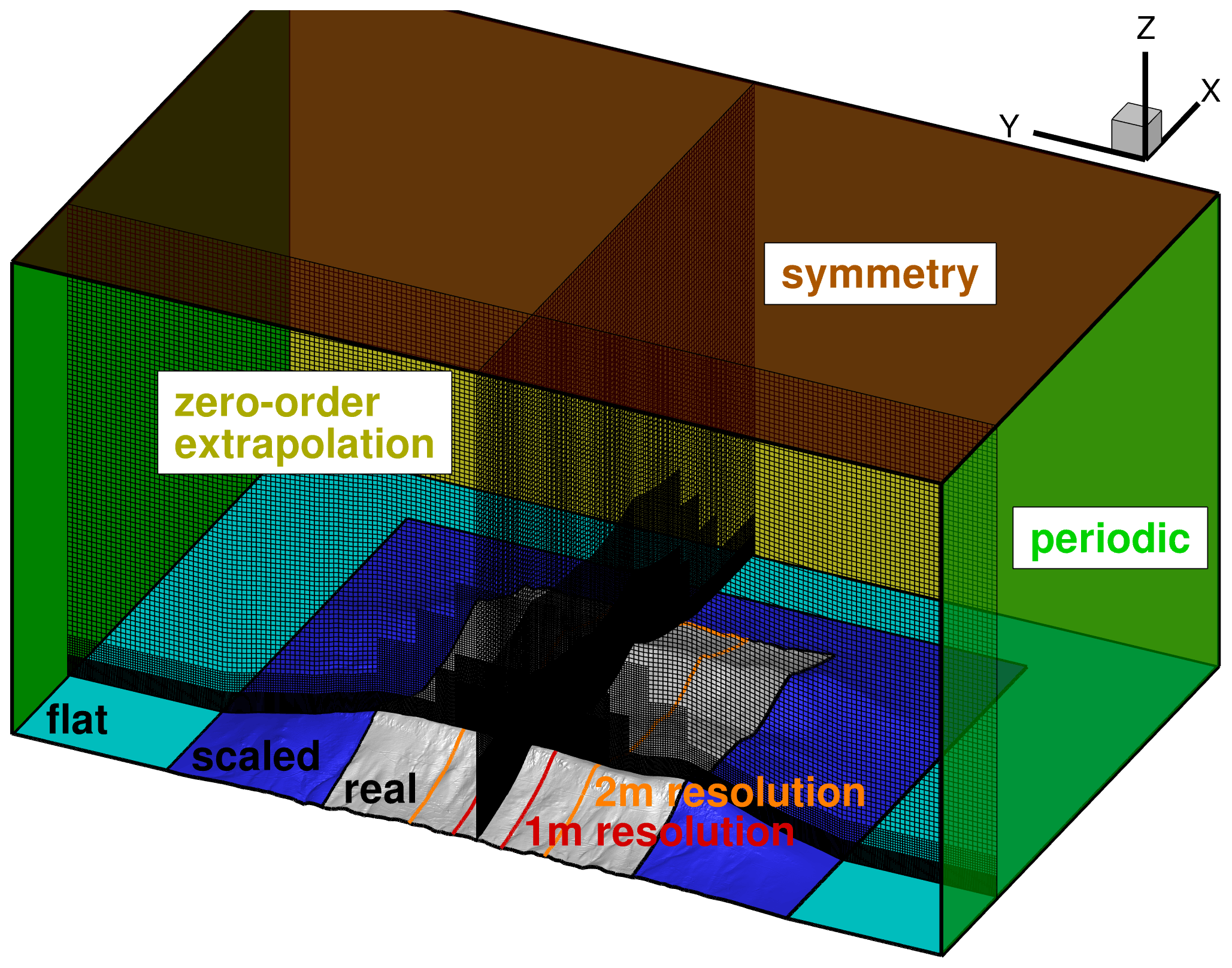
Figure 2 CFD domain for the FLOWer simulation of the complex terrain in Perdigão with boundary conditions and terrain mesh for a wind direction of 230^∘.

The Perdigão terrain mesh is shown in Fig. 2. It is created using cubic cells with a resolution of Δ₀=1 m around the turbine and its direct inflow (−768 m $<x<$ 512 m, −160 m $<y<$ 160 m, z<256 m a.g.l., marked with red lines). The cells are slightly stretched or squeezed in the z direction and skewed to follow the terrain. This resolution is sufficient to resolve the ambient turbulence with an integral length scale $L>\mathrm{20}{\mathrm{\Delta }}_{\mathrm{0}}=\mathrm{20}$ m, following Kim et al. (2016). This region is embedded in a band ($y=\pm \mathrm{448}$ m) with 2 m resolution that covers both ridges and resolves detailed terrain features (marked with orange lines in Fig. 2). A coarsening of the mesh towards the domain boundaries is applied using hanging grid nodes to reduce the number of cells and to dissipate the turbulence towards the BCs for stability reasons. Close to the ground (no-slip wall), BL cells with smaller vertical extent (growth rate of 1.12) are included to ensure $y^{+}<\mathrm{5}$ in the region of interest. This is crucial since without BL cells the Menter SST k−ω RANS model remains in k–ε mode even in the first wall-normal cells (switch to k–ω only for $y^{+}<\mathrm{70}$; Leschziner, 2015). Moreover, the DDES shielding fails without BL cells and the modelled stresses are depleted, which can lead to grid-induced separation on the ridge. Overall, the Perdigão terrain mesh consists of 242 million cells.

3.2.2 Vegetation in FLOWer

Menke et al. (2020) discussed how sensitive the simulation result is with respect to the forest parametrization. They found that the standard forest height h=30 m often used in simulations causes too much drag. For this reason, an accurate representation of the forest upstream of the turbine is targeted. In FLOWer the model of Shaw and Schumann (1992) is applied, which is based on the expression

$$\begin{array}{}\text{(1)}& F_i\left(z\right)=-c_{\mathrm{d}}\mathrm{LAD}\left(z\right)\mathrm{|}{u}_i\mathrm{|}{u}_i.\end{array}$$

The drag force F_i in the direction i depends on the two forest characteristics c_d, a constant drag coefficient and the leaf area density profile LAD(z). Moreover, it scales with the local flow velocity u_i squared. The drag coefficient c_d is set to 0.15 as proposed by Shaw and Schumann (1992). The LAD profile which characterizes the tree type is approximated on the basis of the leaf area index LAI according to Lalic and Mihailovic (2004). They derived the empirical leaf area density distribution function

$$\mathrm{LAD}\left(z\right)={\mathrm{LAD}}_{\mathrm{m}}{\left({\displaystyle \frac{h-z_{\mathrm{m}}}{h-z}}\right)}^n\exp \left[n\left({\displaystyle \frac{h-z_{\mathrm{m}}}{h-z}}\right)\right],$$

with

$$\begin{array}{}\text{(2)}& n=\left\{\begin{array}{ll}\mathrm{6}& \mathrm{0}\le z<z_{\mathrm{m}}\\ \mathrm{0.5}& z_{\mathrm{m}}\le z\le h\end{array},\right.\end{array}$$

where h is the tree height and LAD_m the maximum value of LAD at the corresponding height z_m.

The tree height h and the leaf area index LAI are included in the available maps for the site in Perdigão (Palma et al., 2020). The tree types growing in Perdigão are eucalyptus and pines (Mann et al., 2017). Lalic and Mihailovic (2004) show that their model fits measured leaf area density distributions of pine forests well with the maximal LAD at z_m=0.6h. With this assumption the maximal leaf area density value LAD_m is obtained by substituting Eq. (2) into Eq. (3) and numerically solving the integral for LAD_m:

$$\begin{array}{}\text{(3)}& \mathrm{LAI}=\underset{\mathrm{0}}{\overset{h}{\int }}\mathrm{LAD}\left(z\right)\mathrm{d}z.\end{array}$$

The contour plot of the tree height in the area upstream of the turbine for WD=230^∘ in Fig. 3a shows many small clusters with different heights. The implementation of the forest model in FLOWer (Letzgus et al., 2018) expects separate forest meshes when the forest characteristics change in the flow direction, making it unsuitable for small clusters. Therefore, the small clusters are combined into six forest patches which are included in the simulation as depicted in Fig. 3b. The lowest relevant tree height is chosen to be 8 m. All areas with a tree height within ±20 % of this height are binned. Then a patch is created that envelopes all collected areas. Small gaps between collected areas are closed, and small distant clusters are neglected. This process is repeated two more times with the subsequent tree height ranges (12 m ± 20 % and 18 m ± 20 %). The procedure allows us to obtain several separate patches with the same tree height if they are all large enough but too far apart to be merged. After all patches are defined, the mean tree height and the mean LAI are calculated for each of them. With Eqs. (2) and (3) and z_m, the LAD distribution can be defined. The forest definition used in the simulation is summarized in Table 1.

Figure 3 Tree height in the area upstream of the turbine for a wind direction of 230^∘ (a) and forest patches included in simulation (b).

Table 1 Tree height h, leaf area index LAI, maximal leaf area density LAD_m and corresponding height z_m for each forest patch.

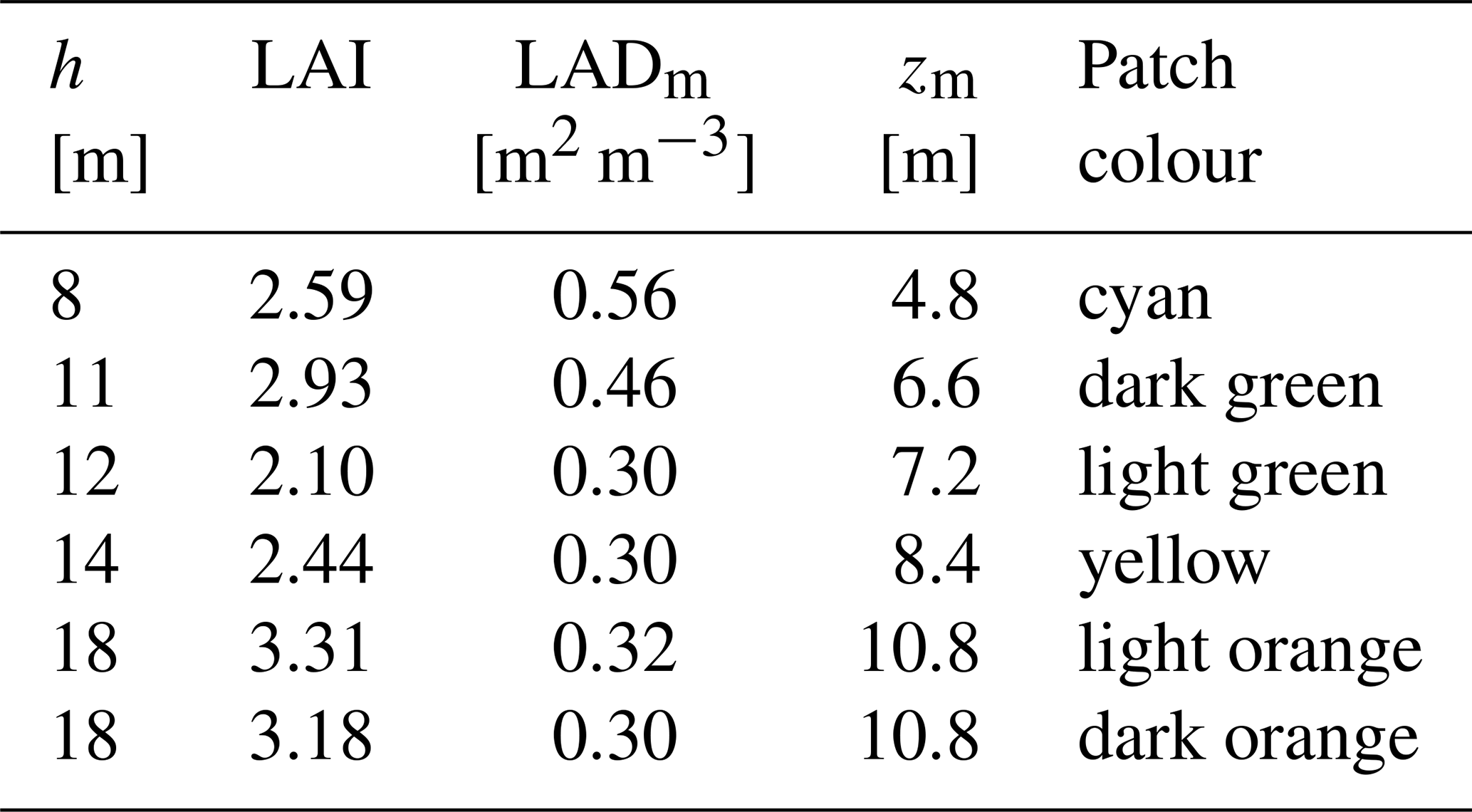
Colours refer to Fig. 3b.

3.3 Atmospheric–aerodynamics interface

From the steady-state flow field of the E-Wind simulation, a slice is extracted at the position of the FLOWer domain inlet (perpendicular to WD=230^∘). The three velocity components (longitudinal u, lateral v and vertical w), the turbulence kinetic energy k and the rate of dissipation ε are averaged in the lateral direction (±100 m relative to the turbine) for each height above the ground. These values are used to create the inflow for FLOWer.

Figure 4 shows the velocity profiles of all three components above ground level (a.g.l.) as derived from E-Wind (dashed lines). The profiles of all velocity components are approximated by piecewise-defined functions (solid lines) such that they resemble the results of E-Wind at the lower part and are constant (u, v) or zero (w) towards the upper boundary. The functions are prescribed at the FLOWer inlet as the Dirichlet BC. In this way, the vertical wind shear, the vertical wind veer and the flow inclination are taken into account. The inlet of the simulation with FLOWer is already in the uneven terrain at the base of the first ridge (inclination ≈ 6^∘). Therefore, it is crucial to prescribe the vertical velocity component w(z) in order not to overestimate the speed-up at the ridge by deflecting the flow too much.

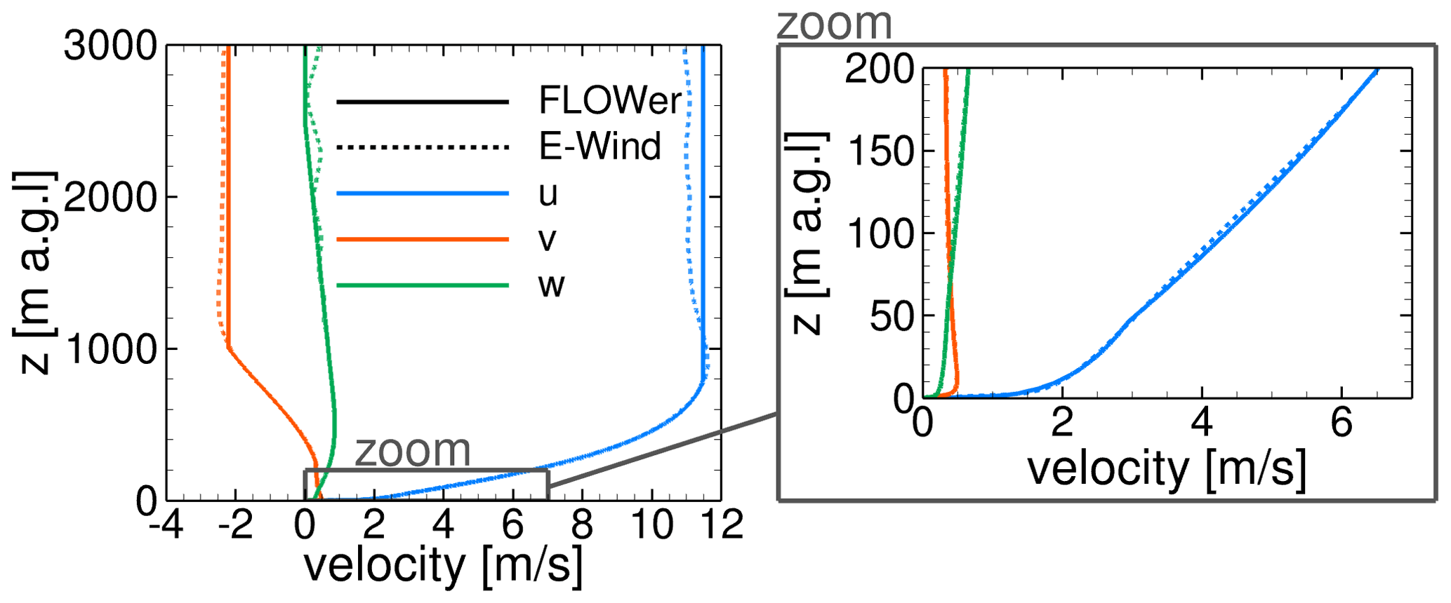
Figure 4 Mean velocity profiles at the FLOWer inlet for the entire height of the domain and zoomed in to near ground level, as extracted from E-Wind and approximated for FLOWer input.

The turbulence intensity TI and the turbulent length scale L of the inflow are calculated from the turbulence quantities k and ε modelled in E-Wind at 77 m a.g.l. (laterally averaged) according to

$$\begin{array}{}\text{(4)}& \mathrm{TI}={\displaystyle \frac{\sqrt{\frac{\mathrm{2}}{\mathrm{3}}{k}_{z=\mathrm{77}\mathrm{m}}}}{\sqrt{u_{z=\mathrm{77}\mathrm{m}}^{\mathrm{2}}+v_{z=\mathrm{77}\mathrm{m}}^{\mathrm{2}}}}}\cdot \mathrm{100}\mathit{\%}\end{array}$$

and

$$\begin{array}{}\text{(5)}& L={\mathrm{0.09}}^{\mathrm{4}/\mathrm{3}}{\displaystyle \frac{k_{z=\mathrm{77}\mathrm{m}}^{\mathrm{3}/\mathrm{2}}}{{\mathit{\epsilon }}_{z=\mathrm{77}\mathrm{m}}}}.\end{array}$$

The resolved atmospheric turbulence for the FLOWer simulation is created using Mann's model (Mann, 1994) and is injected using a momentum source term (Troldborg et al., 2014), superimposing the steady inflow profiles at a distance of L from the inlet. To comply with the atmospheric conditions according to IEC 61400-1 (2019), anisotropic turbulence is generated. As recommended by Mann (1998), the stretching factor in the model is chosen to be Γ=3.9 to approximate the Kaimal spectral model. It is ensured that the dimension of the Mann box is larger than 8L in all directions and that its resolution is smaller than $L/\mathrm{8}$.

The injection via forces as well as the numerical dissipation due to the resolution of the meshes causes a certain turbulence decay within the CFD simulation. This effect is taken into account by applying a scaling factor f_CFD=1.4 to the velocity fluctuations of the Mann box, following Kim et al. (2016), for a propagation distance of approximately 20L.

3.4 Turbine

The examined WT is a generic 2 MW turbine named I82 (Arnold et al., 2020) with aero-servo-elastic similarity to the commercial turbine at the site. The turbine has a hub height of 77 m and a rotor radius of R=41 m. The blades are pre-bent (−1.8 m at the tip) and feature winglets. The rotor is mounted with a tilt angle of 5^∘ and a pre-cone angle of 0^∘. The tower has a bottom diameter of d_b=4.3 m and a top diameter of d_t=2.0 m.

3.4.1 CFD model in FLOWer

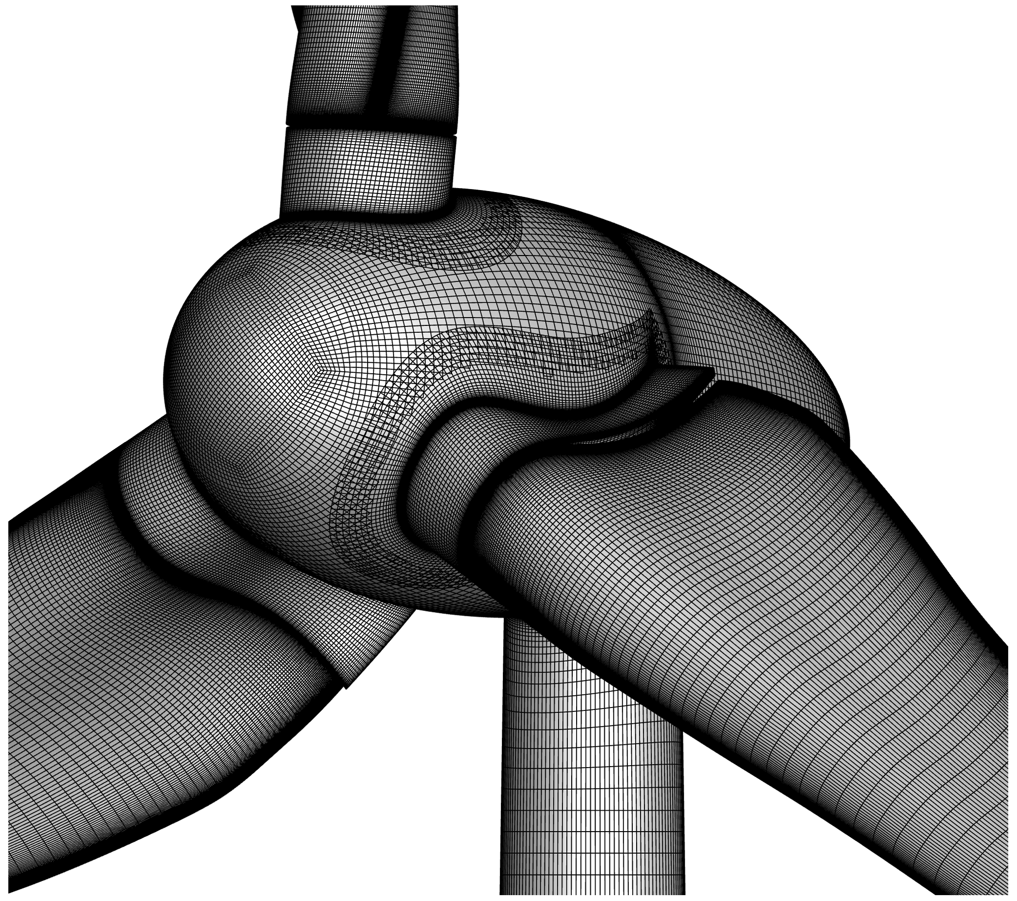
The unsteady FLOWer simulations of the turbine are based on the process chain established by Klein et al. (2018). The CFD model of the I82 turbine for the simulation with FLOWer consists of 17 independent meshes, which are embedded in the Perdigão terrain mesh or a flat background mesh. Three blade tip refinements and a rotor disc refinement comprise the turbine component meshes, namely lower tower, upper tower, nacelle, hub, blade–hub connectors (3×), blades (3×) and winglets (3×). There are no gaps between the turbine components (see Fig. 5), and the BL of all components is fully resolved ($y^{+}<\mathrm{1}$). The blades are meshed in an O-type topology based on the guidelines of Vassberg et al. (2008), with a special focus on a good resolution of the BL and the blade wake.

Figure 5 CFD surface mesh of the hub region, showing mesh overlapping.

Three differently resolved blade meshes are used to conduct a grid convergence study following Roache (1994) ($y^{+}<\mathrm{1}$ is kept in all blade meshes). The conservative numerical error for the medium blade mesh (${\mathrm{GCI}}_{\mathrm{coarse}}^{\mathrm{21}}$) is 0.4 % for thrust and 0.6 % for torque. This is acceptable, and hence the blade mesh with medium resolution is chosen, with 192 cells in the radial direction, 304 cells around the airfoil, 64 cells on the trailing edge and 144 wall-normal cells, resulting in 11.4 million cells per blade. The growth rate in the BL is 1.09. The second-order JST scheme is used for spatial discretization in the component meshes. The numerical settings of the complex-terrain simulation without the turbine are kept, but the time step is reduced.

3.4.2 Structural model in SIMPACK

Klein et al. (2018) show that the blade–tower interaction, a key mechanism investigated in the following, is dominated by the blade–tower distance, which is massively reduced when the aeroelasticity of the blades is taken into account. The structural model of the I82 turbine in SIMPACK is adopted from Arnold et al. (2020). The blades are modelled as nonlinear beams using 29 flexible beam elements (Timoshenko) per blade with Rayleigh damping. The tower is adjusted to a steel tower and modelled as a linear beam by using 77 flexible beam elements (Euler–Bernoulli) with a modal damping of ζ=0.002. All eigenfrequencies below 15 Hz are considered in SIMPACK. The hub, nacelle, drive train and foundation are defined as rigid bodies. The centrifugal force induced by the blade rotation and the gravity force are considered. A variable step-size integrator is used to ensure that at each time step all model states are kept within predefined tolerances.

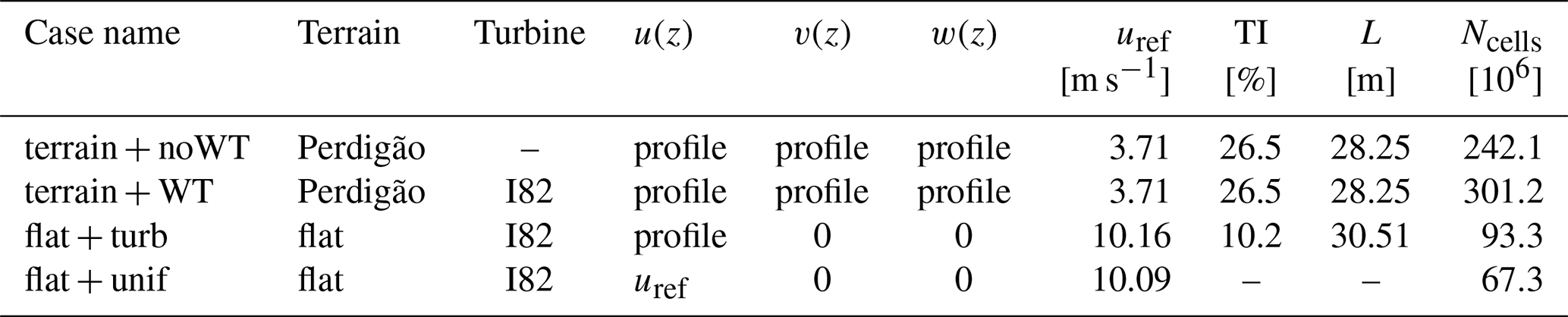
Table 2 Definition of FLOWer simulation cases with their inflow conditions and mesh size.

3.4.3 Fluid–structure coupling

An explicit coupling scheme is applied between SIMPACK and FLOWer with both solvers running in a sequential way. After each physical time step, information is exchanged, with SIMPACK using the aerodynamic loads of the previous time step to calculate the deformations. The communication is realized by means of files containing deformations or loads at a total of 106 marker positions, of which 29 markers are allocated to each blade, 17 markers to the tower, and 1 marker each to the nacelle and hub. The surface mesh is reduced to a point cloud that deforms according to the markers. The cells of the volume mesh are linked to the point cloud via radial basis functions and thus also deform accordingly. Further details can be found in Klein et al. (2018) and a validation of the FLOWer–SIMPACK coupling with an elastic cantilever beam in Klein (2019).

3.5 Simulation cases

To validate the wind field simulated with FLOWer, the complex terrain in Perdigão is simulated without the turbine, as described in Sect. 3.2. After the initialization, 180 s is simulated to be evaluated. This simulation is referred to as the terrain + noWT case.

The terrain + noWT case is also the basis of the simulation with the turbine I82 in the complex terrain, referred to as the terrain + WT case. The turbine with its multiple component meshes is integrated into the Perdigão terrain mesh with the propagated turbulent terrain flow (after 300 s). A total of 16 revolutions without fluid–structure coupling are simulated with a time step corresponding to 2^∘ azimuth to reduce the disturbances due to the integration and to develop the turbine wake. Then two revolutions are simulated with FSI to obtain the quasi-steady deformation of blades and tower. A calibrated artificial damping is applied to attenuate the starting oscillations due to the uninitialized structural model. For the evaluation simulation, the artificial damping is switched off and the time step is reduced so that it corresponds to 1^∘ azimuth. The turbine is simulated with a constant rotational speed of n=16.87 rpm, which corresponds to the 30 min average (10 May 2017 from 15:15:00 UTC) of the turbine's rotational speed at the site. The corresponding pitch angle of the generic I82 is β=4.06^∘.

The two reference simulations with FLOWer of the I82 in flat terrain use the same operating conditions and are also run as coupled simulations. One simulation, referred to as flat + turb, has a turbulent inflow with vertical wind shear. It is created using the method described in Sect. 3.3. However, for this case, the E-Wind results are taken from a slice at the turbine position at the top of the ridge. Hence, the effects of orography and vegetation on the horizontal wind speed WS, TI and L are only included in the FLOWer input to the extent that E-Wind is able to reproduce them. The vertical velocity component occurring at the turbine position is neglected in this setup. The second reference simulation, referred to as flat + unif, has a uniform inflow. The wind velocity is taken from the E-Wind result at hub height and is 10.09 m s⁻¹. The flat background meshes for the reference simulations are 50 rotor radii (R) long (12.5R upstream of the rotor plane) and 25R wide and high. For turbulent inflow, a no-slip wall and BL cells are used at the bottom, and for uniform inflow, a slip wall and no BL cells are used.

The four simulation cases with the respective inflow conditions are summarized in Table 2, with the longitudinal velocity u_ref, TI and L as reference values at the inlet at 77 m a.g.l. The overall number of cells N_cells per setup is also given.

4 Results part 1 – terrain flow in Perdigão

The validation of the flow field in the complex terrain at Perdigão simulated with E-Wind as well as with FLOWer is presented in the first part of the results. This demonstrates the suitability of the process chain for the detailed simulation of the complex terrain. Two lidar planes (Menke et al., 2019; UCAR/NCAR, 2019a) and the three met masts (UCAR/NCAR, 2019b) shown in Fig. 6 are used for validation (30 min average).

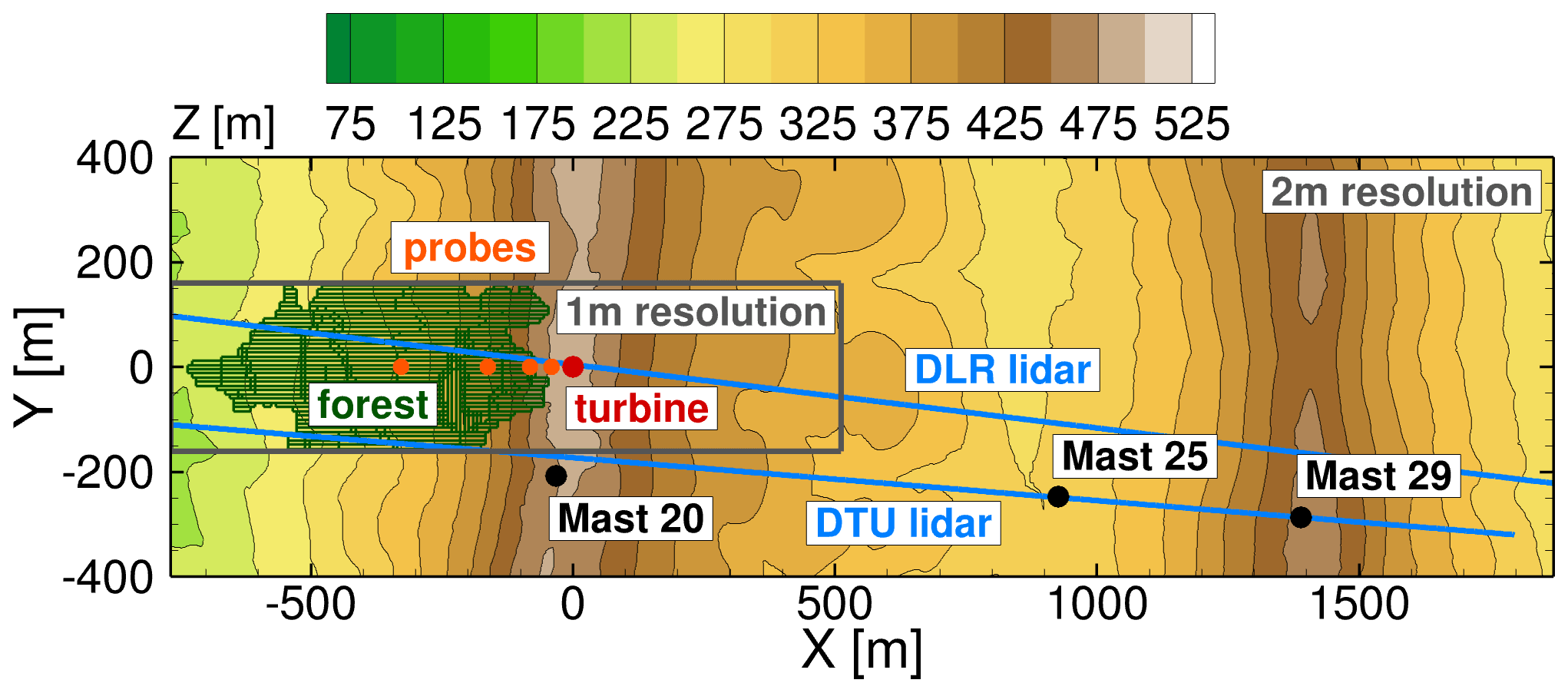
Figure 6 Location of lidar planes, met masts and probe positions in Perdigão relative to the turbine and properties of the FLOWer setup.

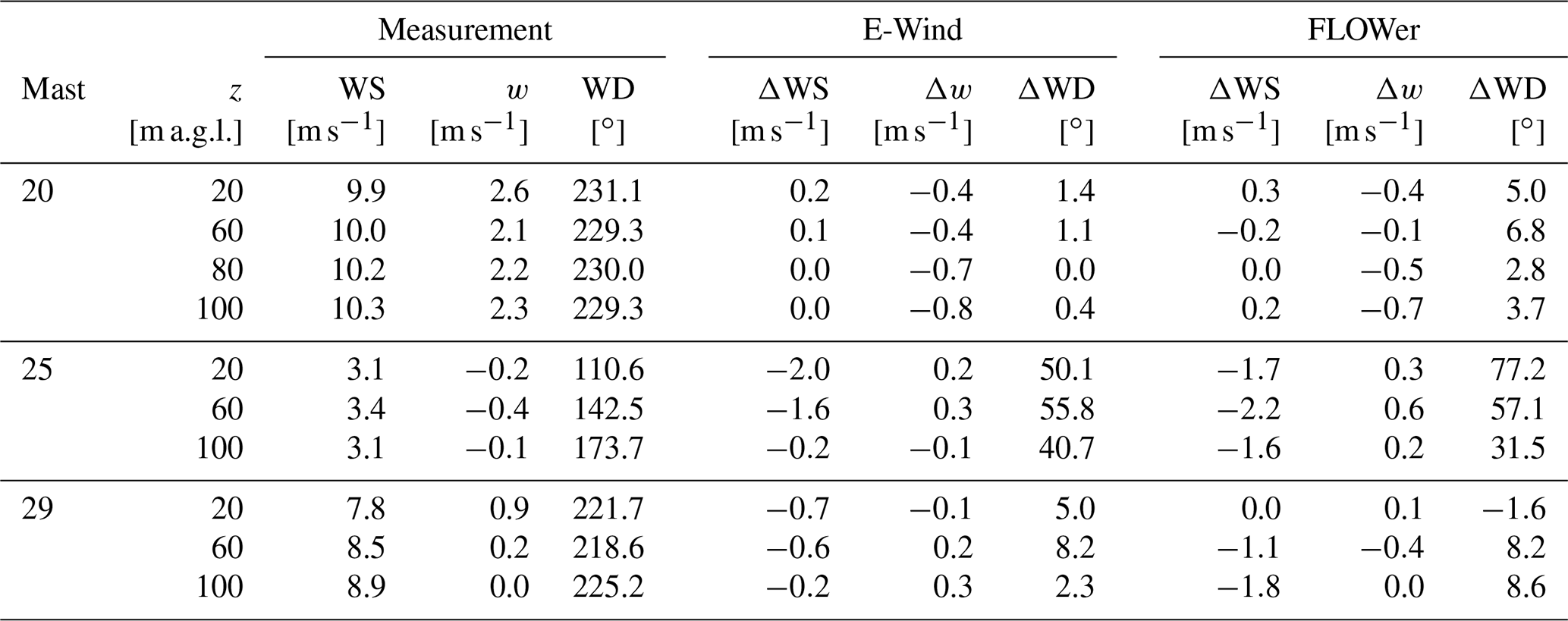
Table 3 Comparison of E-Wind result and FLOWer result (180 s averaged) with met mast data (30 min averaged).

$\mathrm{\Delta }=\mathrm{simulation}-\mathrm{measurement}$.

Figure 7 Comparison of the horizontal component of the line-of-sight velocity in the DTU lidar plane between the E-Wind result and the measurement.

4.1 Validation of precursor simulation (E-Wind)

The measured horizontal wind speed, vertical velocity and wind direction at the met masts at three heights and the deviation of the flow field simulated with E-Wind are listed in Table 3. At mast 20, which is used for calibration, a very good agreement between simulation and measurement with respect to mean wind speed and wind direction is achieved (see Table 3). Figure 7 shows the difference in the horizontal component of the line-of-sight velocity u_h in the Technical University of Denmark (DTU) lidar plane between the E-Wind result and the lidar measurement. The x axis describes the distance from mast 20 in the lidar plane. Only minor differences are observed in front of the first ridge, which justifies the extraction of the data for the generation of the inflow for the FLOWer simulation from the precursor simulation at the base of the first ridge.

The recirculation zone behind the first ridge is strongly underpredicted in E-Wind. The main reason is probably the smoothing of the terrain due to the mesh resolution of 10 m. Satellite images of the site show rocky terrain at the top of the ridge that could trigger early flow separation. Since these terrain features are not resolved in E-Wind, the flow stays attached to the ground longer and separates later, resulting in a smaller recirculation region. Moreover, it is well known that RANS models have difficulties in accurately predicting the size of and the flow within a recirculation zone. Consequently, large differences between simulation and measurements are observed in the valley at mast 25, especially at the lower heights. WS is underestimated and WD is off by about 50^∘ in the simulation. Other reasons for the large deviations may lie in some microscale or other physical effects that are not modelled in E-Wind (e.g. anabatic winds). At mast 29 on the second ridge, a better agreement with the measurements can again be observed.

4.2 Validation of unsteady simulation (FLOWer)

The results of the DDES with FLOWer of the wind field in Perdigão without the turbine (case terrain + noWT) are averaged for 180 s (equivalent to 3 times the duration of the Mann turbulence box) and compared with measured data. Figure 8 shows the simulated mean horizontal component of the line-of-sight velocity in the DTU lidar plane u_h of the terrain + noWT case and the difference from the measurement. The speed-up at the first ridge agrees very well with the measurement, which is important to simulate the local flow at the turbine position correctly. The velocity in the recirculation zone is captured much better than in the steady-state precursor simulation with E-Wind, but still the differences in the valley between the ridges are the largest.

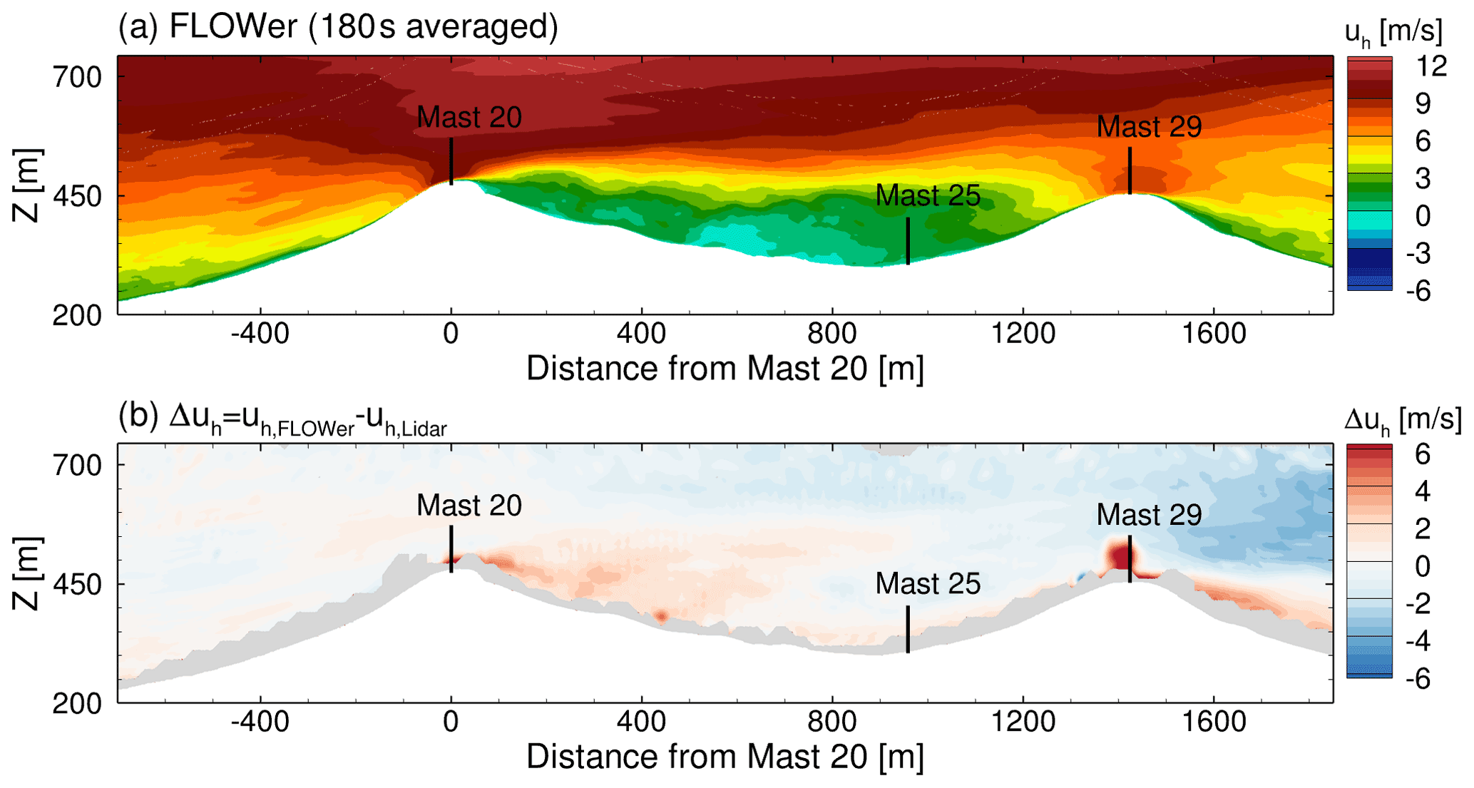
Figure 8 Horizontal component of the line-of-sight velocity in the DTU lidar plane, simulated with FLOWer (a) and difference from measurement (b).

A comparison with the met mast data in Table 3 confirms this. At mast 20, both the horizontal wind speed WS and the wind direction WD match very well over the entire mast height, indicating that the vertical wind shear is met. The vertical velocity w and thus the flow inclination is slightly underpredicted. The turbulence intensity cannot be compared at the position of the met masts because none of them is located in the finest mesh region of the simulation (compare Fig. 6), and therefore the numerical dissipation has strongly damped the resolved turbulence there. Nevertheless, to get an indication of the quality of the simulated turbulence, the intensity measured at mast 20 at 80 m a.g.l., ${\mathrm{TI}}_{\mathrm{mes},\mathrm{mast}\mathrm{20}}=\mathrm{11.4}$ %, is compared with the simulated TI one rotor radius in front of the turbine (see probe in Fig. 6) at 77 m a.g.l., ${\mathrm{TI}}_{\mathrm{sim},x=-R}=\mathrm{8.8}$ %. The simulated TI is slightly too low, showing that the turbulence decay during the propagation from the injection plane to the turbine position is not fully compensated for by f_CFD (see Sect. 3.3). Mast 25 in the valley shows large differences, especially in the wind direction. This is probably due to a thermally driven valley flow (Fernando et al., 2019), whose physical source is included neither in the FLOWer simulation nor in E-Wind. This missing flow also causes the wind speed to be too low. On the second ridge at mast 29, the agreement between simulation and measurement is better again. The too low WS, which can also be seen in Fig. 8, might be due to too small a distance of the second ridge to the outlet BC in the simulation, where vortices that are not fully dissipated can cause a backward inflow.

The energy-containing vortices in the simulation of the flow over the terrain in Perdigão are identified by calculating the power spectral density (PSD) using Welch's method with the Hann window (amplitude corrected), 66 % overlap and three segments. The horizontal velocities at four positions at 77 m a.g.l. in the direct inflow of the turbine position (see probes in Fig. 6) are evaluated. Figure 9 shows the spectra compared to the measurement at mast 20 at a height of 80 m a.g.l., where the energy cascade is proportional to $f^{-\mathrm{5}/\mathrm{3}}$ as given by Kolmogorov for the inertial subrange. The simulation resolves this energy cascade for more than an order of magnitude before numerical dissipation causes a drop for frequencies f>1 Hz. The resolved part of the spectrum covers the relevant load range for WTs since the blade-passing frequency (BPF) for the turbine integrated into the terrain later in the simulation corresponds to f_BPF=0.84 Hz. Further up the ridge, turbulence with higher frequencies is resolved as the flow accelerates, which agrees with Spalart (2001), who found that the smallest eddies resolvable with DES occur with a frequency of $f_{\max }\approx u\cdot (\mathrm{5}\cdot {\mathrm{\Delta }}_{\mathrm{0}}{)}^{-\mathrm{1}}$.

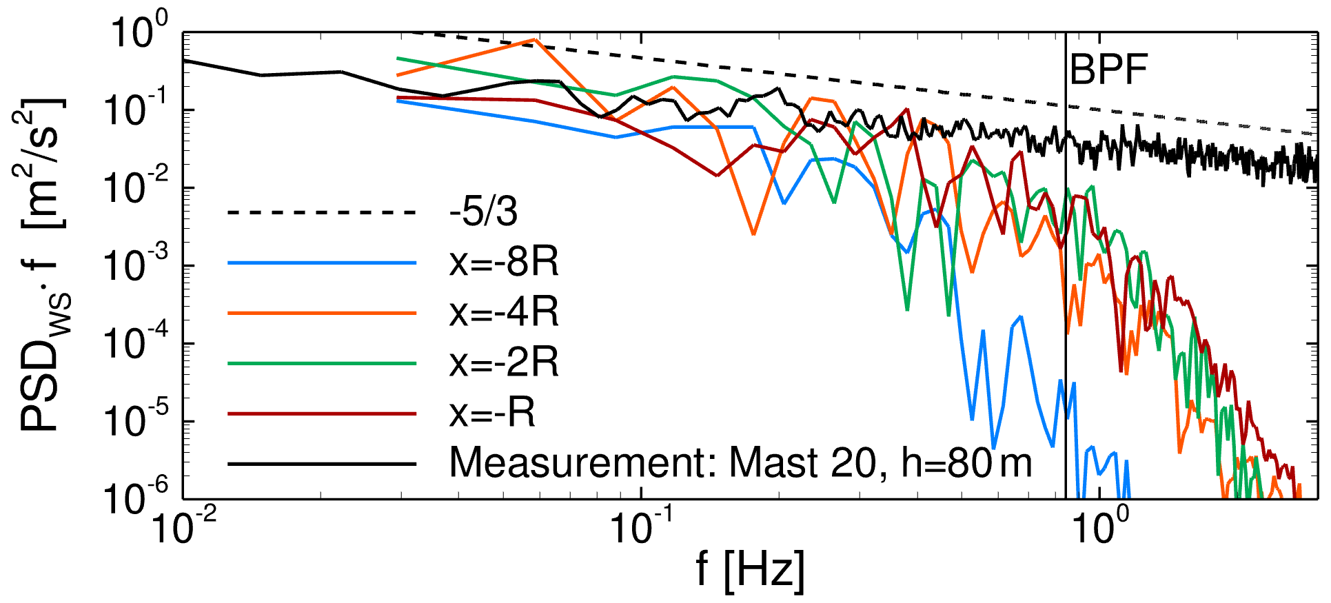
Figure 9 Development of power spectral density of horizontal wind speed upwind of the turbine at 77 m a.g.l. in FLOWer.

It can be concluded that the DDES of the complex terrain in Perdigão with FLOWer using the inflow generated from E-Wind results gives a realistic flow field on the first ridge. There, both the mean flow field and the resolved turbulence spectrum up to f≈1 Hz agree with lidar and met mast data, even if the turbulence intensity is somewhat too low due to numerical dissipation. This ensures that the following studies on the influence of the inflow on the turbine aerodynamics are also applicable to reality. Further downstream, however, in the valley as well as on the second ridge, the simulated flow field deviates from the measured situation due to missing physical phenomena and numerical dissipation.

5 Results part 2 – impact of inflow on turbine aerodynamics

The overall goal of the presented simulation chain is to model surface pressure fluctuations on a WT under realistic operating conditions in complex terrain. In the second part of the results, the fluid–structure-coupled simulation of the I82 turbine in the complex terrain at Perdigão (case terrain + WT) is evaluated for 16 revolutions after initialization of the wake and the deformations as described in Sect. 3.5.

The flow field around the turbine and its global loads and deflections as well as surface pressure fluctuations on blades and tower are investigated. The results are compared with the reference simulations in flat terrain (cases flat + unif and flat + turb).

5.1 Turbine wake in complex terrain

The DLR lidar is in plane with the turbine and orientated almost parallel to the WD_hub of this situation (see Fig. 6) and is therefore well suited to evaluate the impact of the turbine on the flow field. Figure 10a shows the difference between the FLOWer simulation with the resolved turbine (case terrain + WT) and the simulation without the turbine (case terrain + noWT). u_h in the DLR lidar plane is averaged over 16 revolutions and the corresponding 60 s from the terrain + noWT simulation. The upwind induction zone in front of the turbine is relatively small, while the wake is quite distinct up to ≈340 m behind the turbine. The wake does not follow the terrain but drifts slightly upwards. This fits well with the findings of Wildmann et al. (2018) from measurements under neutral stratification; however the velocity deficit decays faster in their study. A comparison with the measured u_h for the selected situation (see Fig. 10b) also shows a faster decay. It should be noted, however, that the DLR lidar plane has an offset of ≈7^∘ from the mean wind direction, which leads to a drift of the wake out of the measured plane. In the simulation, the flow is unintentionally more aligned with the DLR lidar plane, which is evident from the offset ΔWD found for mast 20 in Table 3. Moreover, the too low TI in the simulation causes the wake to be slightly too stable. Overall, the influence of the turbine on the terrain flow is well captured.

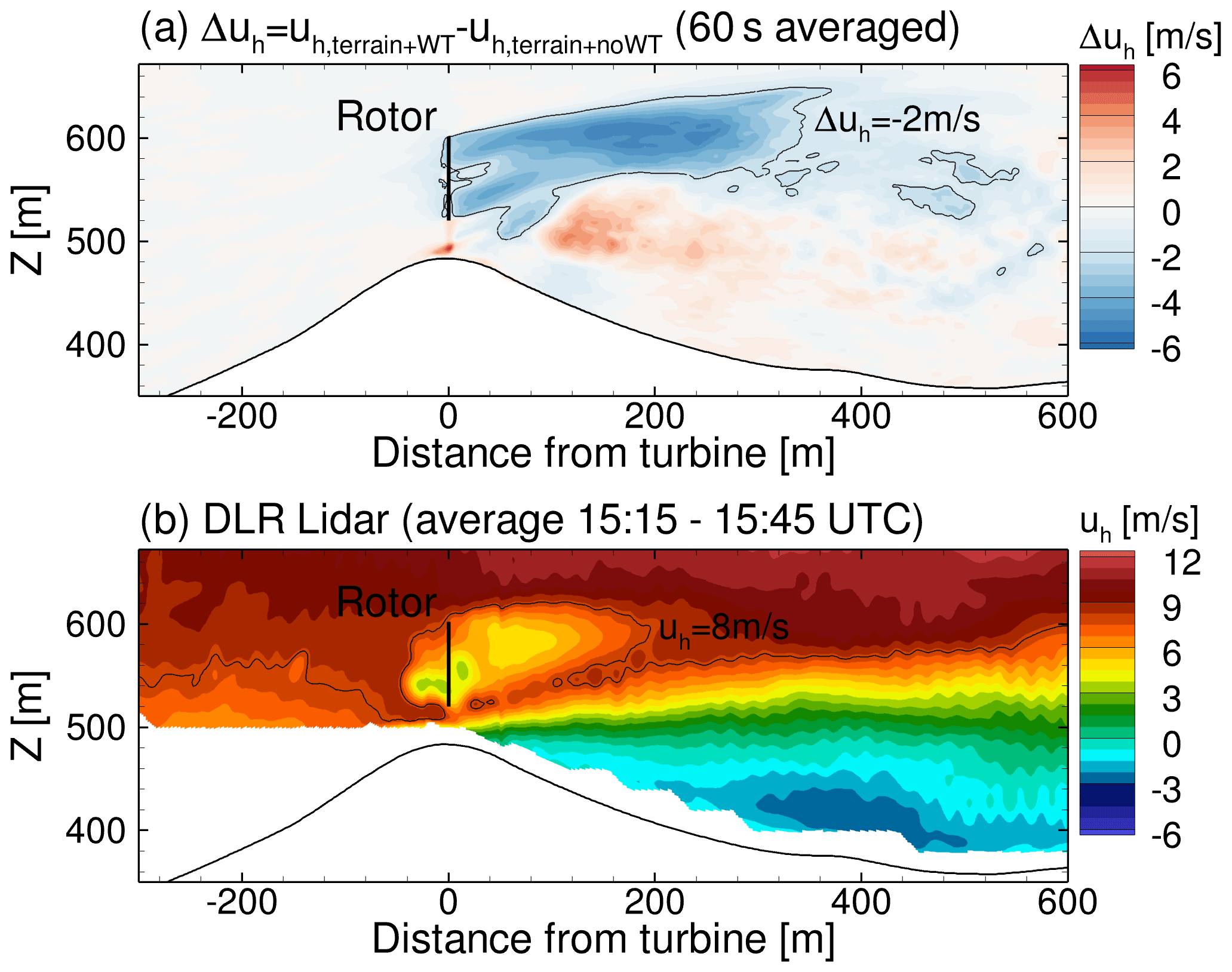
Figure 10 Horizontal component of the line-of-sight velocity in the DLR lidar plane, with the difference between the FLOWer results of the simulation with and without the turbine (a) and measured distribution (b).

5.2 Global loads and deflections

Figure 11 shows the blade tip displacement out of the rotor plane Δx_oop of one blade for all cases. The flat + unif case shows a clear sinusoidal trend mainly caused by the gravity load and the rotor tilt. The blade deformation overcompensates for the pre-bend, so gravity contributes more to the out-of-plane displacement when the blade is pointing upwards. The impact of the blade–tower interaction on the blade deformations is only weakly recognizable by the faster decrease in Δx_oop shortly after the tower passage. The inclusion of turbulence in the reference simulation flat + turb massively increases the amplitude of fluctuations that occur once per revolution. This is due to the large variations in wind speed over the rotor disc arising from vertical wind shear and turbulence. However, the effects of turbulence outweigh those of vertical wind shear, as can be seen from the irregular pattern. The turbulent eddies are smaller than the rotor disc (L<2R) and therefore cause load oscillations with the rotation frequency. Moreover, the rotational periodicity is superimposed by stochastic broadband fluctuations caused by very small eddies. A comparison between the flat + turb and the terrain + WT case shows that the inflow turbulence cannot be generalized and has a unique impact on the loads and deformations of the blades in each case. This illustrates how important it is to model the inflow realistically and site specifically.

Figure 11 Deformation of blade tip out of the rotor plane Δx_oop for all cases.

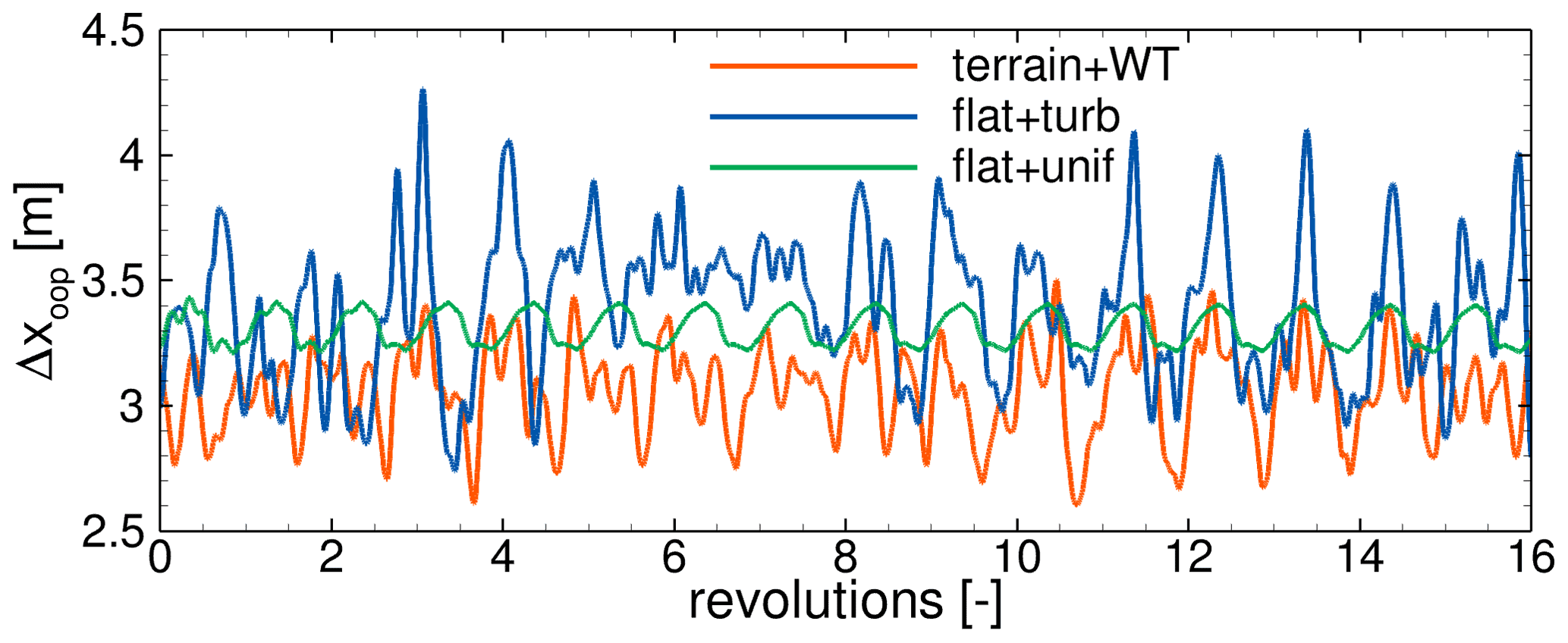
The differences in the mean blade tip deformation ${\stackrel{\mathrm{‾}}{\mathrm{\Delta }x}}_{\mathrm{oop}}$, given in Table 4, are due to differences in the global loads caused by slightly different flow conditions at the turbine position in the three simulations. Table 4 also lists the local inflow to the turbine characterized by a mean velocity U_ref and a mean flow inclination angle γ 1R in front of the turbine at hub height as well as the extracted mean powers $\stackrel{\mathrm{‾}}{P}$ and mean acting thrusts ${\stackrel{\mathrm{‾}}{F}}_x$. The intention has been to obtain similar flow conditions at the turbine position and thus similar loads in the three simulations (compare Sect. 3.5). However, it turns out that the underlying E-Wind results overestimate the velocities at the turbine position. Due to the too small recirculation zone in E-Wind, the streamlines follow the terrain more closely than in FLOWer and are therefore more curved, resulting in greater acceleration. The unsteady aerodynamic effects analysed in the following are not significantly altered by differences in mean loads and can still be compared between the cases.

Table 4 Local inflow to the turbine and global loads on the turbine for all simulation cases.

5.3 Surface pressure on tower

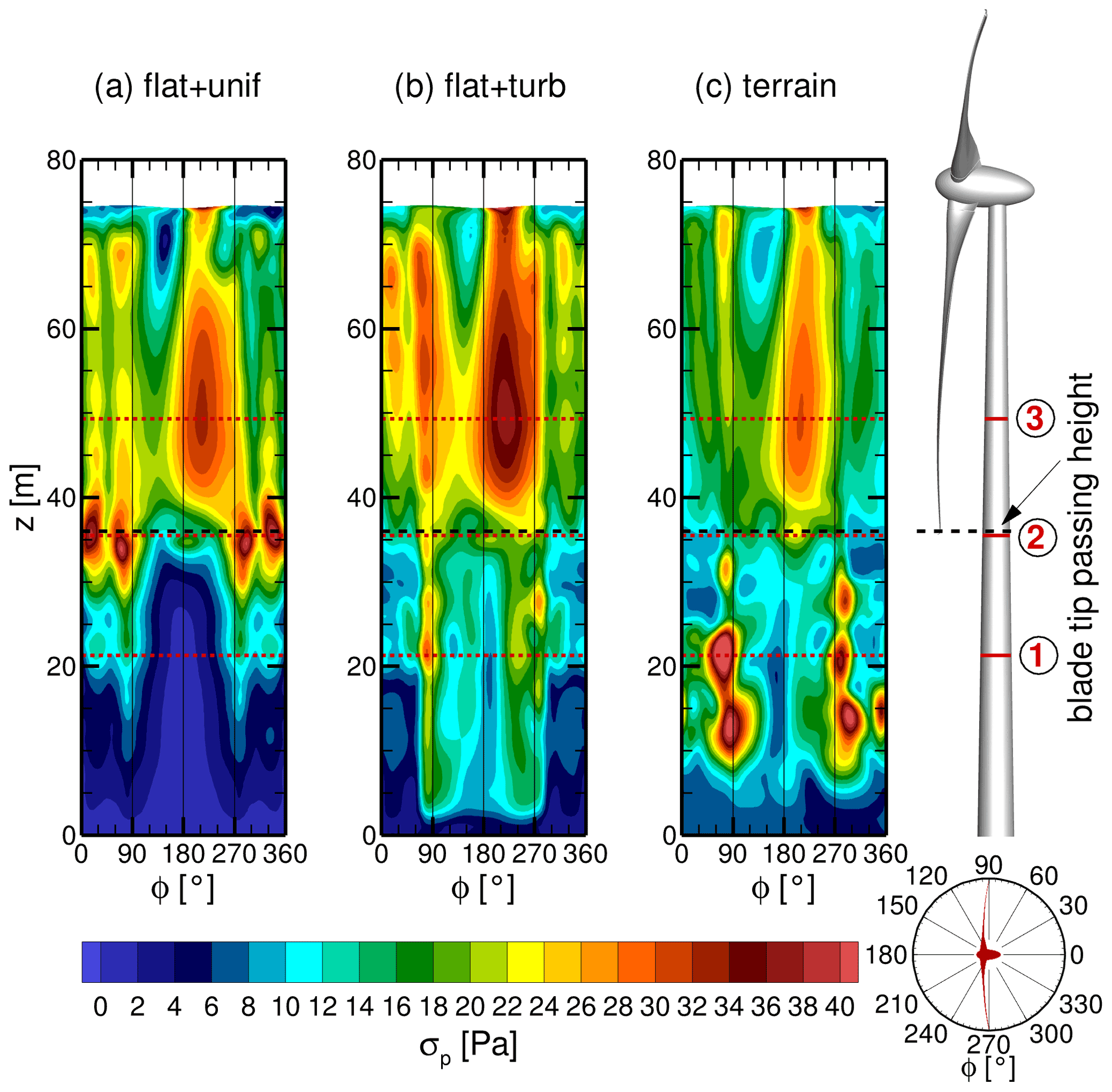
The surface pressure p and its distribution are the dominant source of the aerodynamic loads and are evaluated on the tower in the following. In many respects, be it fatigue loads or acoustic emissions, the fluctuations and the distribution of the acting forces are of greater importance than the magnitude of the steady load. Figure 12 shows contour plots of the standard deviation σ of the surface pressure on the tower for all cases. In the plots the angle Φ on the x axis corresponds to the circumferential position of the tower, where 180^∘ is the upwind side where the blades pass. Three main areas of interest can be distinguished, marked with horizontal dotted lines in red – (1), (2) and (3). Below the blade tip passage (1), inflow turbulence increases the fluctuations, especially in the terrain + WT case, while at the height of the blade tip passage (2), the fluctuations are actually reduced in both cases with turbulent inflow compared to uniform inflow. The main effect of the blade on the tower is at around 50 m height (3) on the side of the descending blade (Φ≈210^∘) for all cases. The cause of these observations is examined separately for each height in the following.

Figure 12 Standard deviation σ of surface pressure p on tower for all cases (a)–(c).

5.3.1 Surface pressure on tower at height (1)

Below the blade passage at height (1), the time series of the surface pressure fluctuations p−p_avg, where p_avg is the local time average, on a line around the tower are extracted and plotted as contour plots in Fig. 13. The uniform inflow causes distinct, periodic patterns, especially on the back and crosswind sides of the tower ($\mathrm{120}{}^{\circ }>\mathrm{\Phi }>\mathrm{240}{}^{\circ }$), which increase in intensity over time. The two cases with turbulent inflow, on the other hand, are dominated by larger patterns that are less regular. Nevertheless, the flat + turb case develops a fine pattern on the tower back after some time. For the terrain + WT case, patterns are by far the largest. Opposing pressure fluctuations occur at the tower sides, which remain stable for multiple revolutions and then swap.

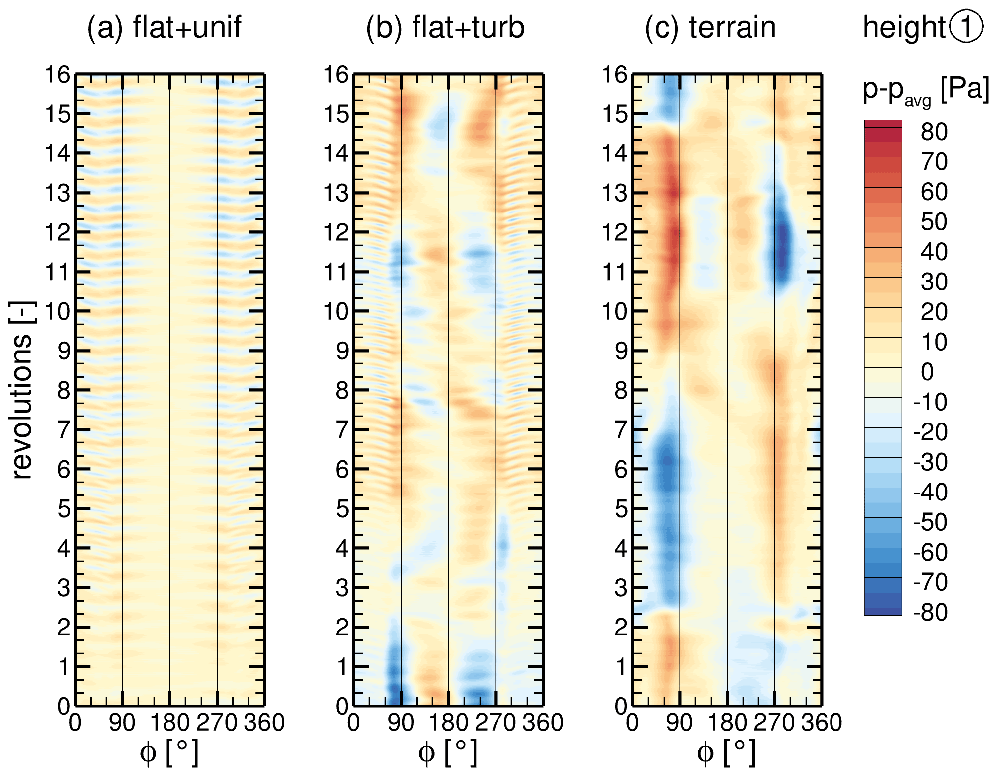
Figure 13 Time series of surface pressure fluctuations p−p_avg on a line around the tower at height (1) for all cases (a)–(c).

With a transformation to the frequency domain using Welsh's method (compare Sect. 4.2), the observed pattern can be better characterized. The PSDs in Fig. 14 show that for uniform inflow, the main fluctuations occur at the tower sides and back at discrete frequencies that are not multiples of the BPF. These pressure fluctuations can be associated with a periodic separation known as the von Kármán vortex street. However, according to Horvath et al. (1986), the local Reynolds number of the tower $Re\approx \mathrm{2.5}\times {\mathrm{10}}^{\mathrm{6}}$ falls into the supercritical regime, where vortex shedding can occur over a wide range of frequencies and is quite unstable or even not observed at all in some experiments. Nevertheless, they found two dominant shedding frequencies in their experiments for supercritical Re numbers. This fits well with the observation in Fig. 14a with two dominant frequencies at f=0.59 and f=1.55 Hz. Considering the time history in Fig. 13, it can even be stated that the shedding characteristic changes over time, which underlines the instability of the vortex street.

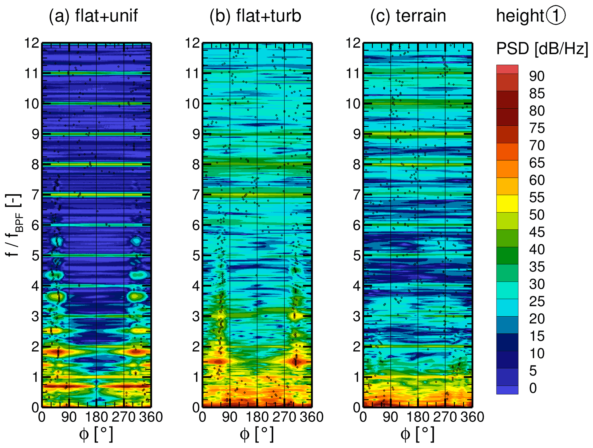
Figure 14 Power spectral density of surface pressure fluctuations on a line around the tower at height (1) for all cases (a)–(c).

Figure 15 shows the instantaneous vortex structures visualized with the λ₂ criterion, coloured with the vertical component of vorticity ω_z. With uniform inflow, coherent vortex cells with constant shedding frequency form and extend over the entire tower height. This phenomenon is well known for tapered cylinders (e.g. Johansson et al., 2015), although it is remarkable that only one vortex cell forms over the entire tower height, not even broken up by the blade tip vortices (not shown). Therefore, using the local tower diameter to calculate the Strouhal number of the shedding frequencies is not appropriate. Using the mean tower diameter gives $St=fd/u=\mathrm{0.18}$, which fits the experimental results of Jones (1968), and St=0.48, which is similar to the higher eddy-shedding frequency measured by Horvath et al. (1986) and simulated by Rodríguez et al. (2015).

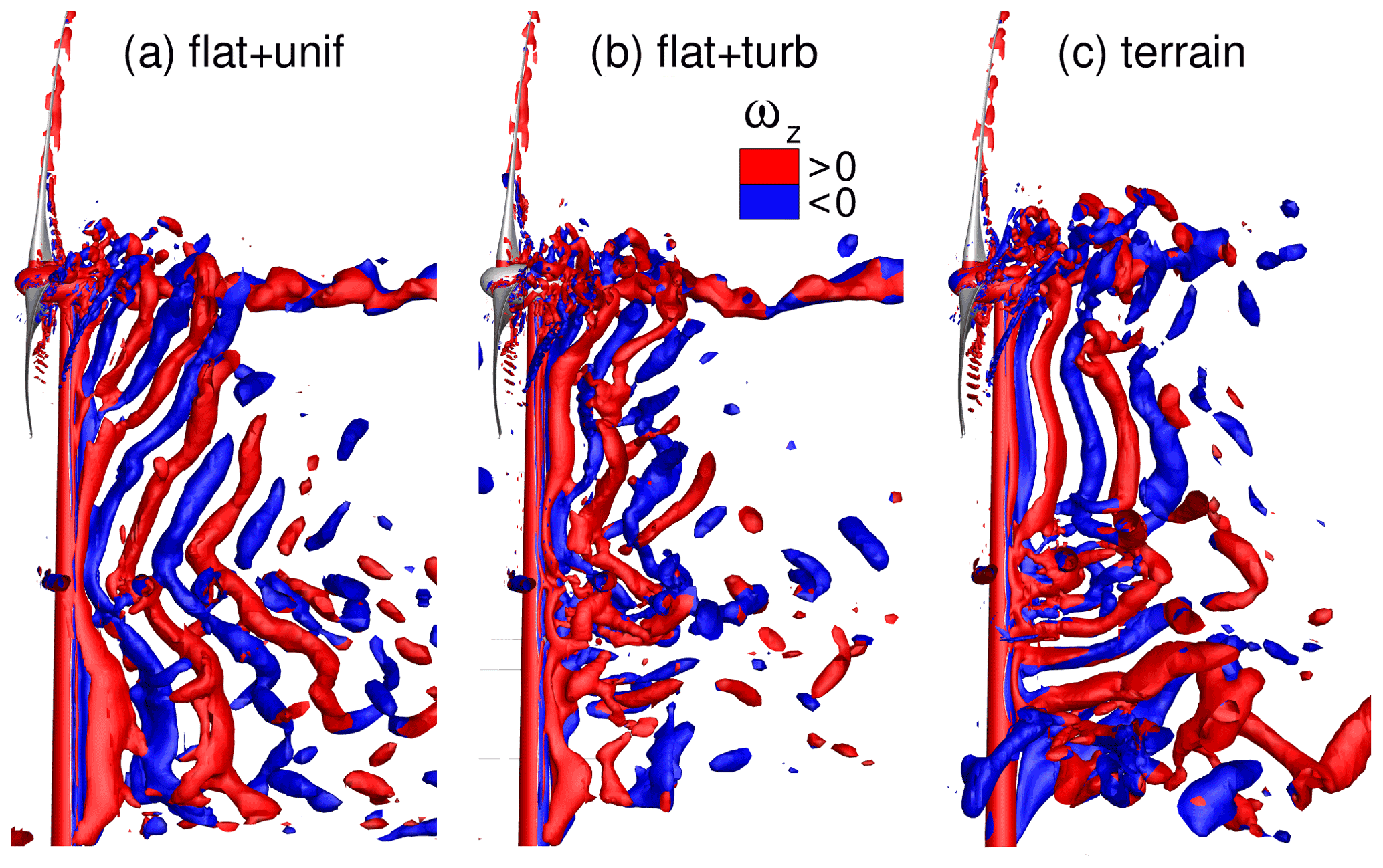
Figure 15 Vortex structures after 16 revolutions visualized with the λ₂ criterion and coloured with vertical vorticity ω_z for all cases (a)–(c).

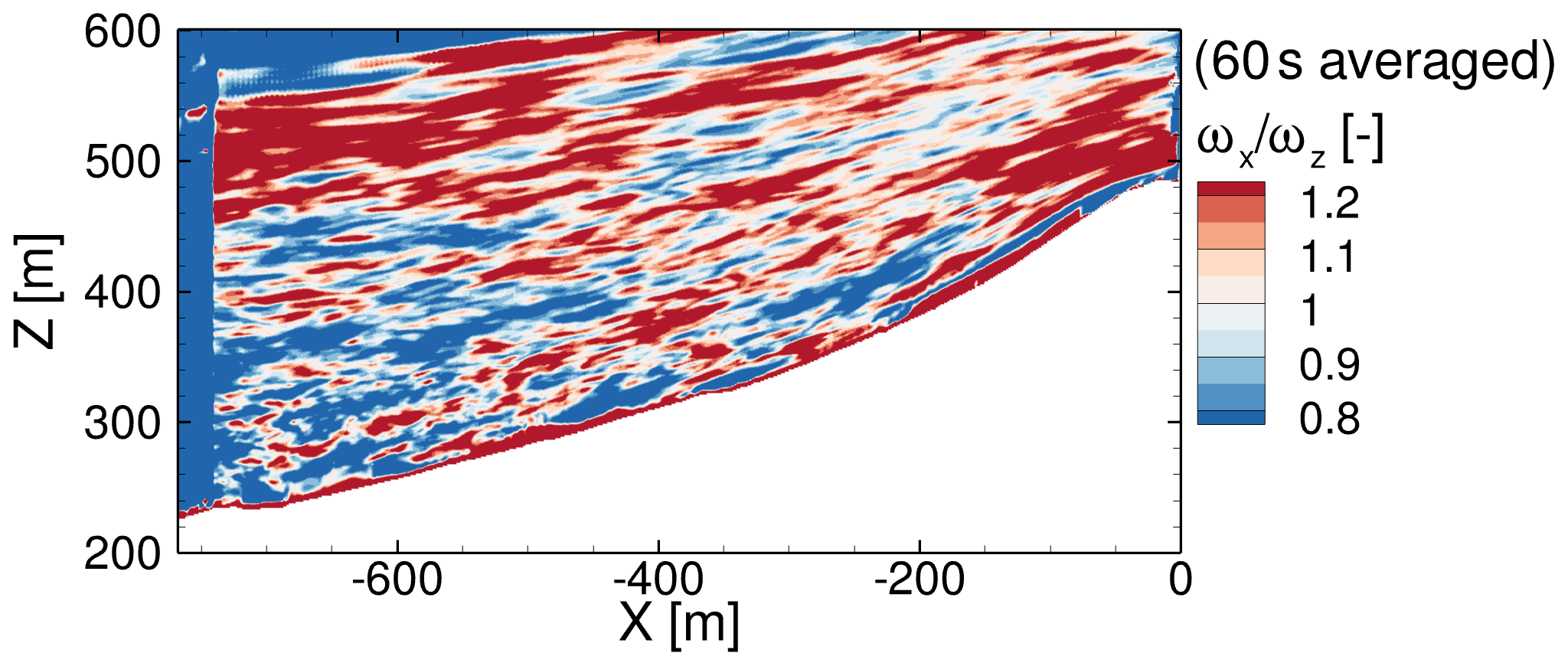
Figure 16 Ratio of horizontal and vertical vorticity ${\mathit{\omega }}_x/{\mathit{\omega }}_z$ in a slice (y=0) upstream of the turbine.

Turbulence in the inflow hampers the periodic vortex shedding at height (1), as shown by the reduction in discrete frequencies in the PSD for the flat + turb case and an absence of discrete frequencies in the terrain + WT case in Fig. 14. The vortex structures in Fig. 15b and c in the lower tower section confirm this. Especially in the terrain + WT case, rather horizontal, streamwise vortex structures tend to occur at the tower and the coherence in the vortex shedding is suppressed in lower tower regions. This vortex shape is triggered by the terrain flow in two different ways. First, the acceleration of the mean flow Δu due to the slope of the ridge rotates and stretches the turbulent structures into rather streamwise vortices. The vertical vorticity ω_z is transferred into ω_x in the near-ground region, as can be seen in Fig. 16 from $x=-\mathrm{200}$ m. Furthermore, the position of the turbulence injection via forces at $x=-\mathrm{768}$ m + $L=-\mathrm{740}$ m is clearly visible from the discontinuity. From there, the resolved turbulence develops rapidly, which can be seen from the directly pronounced anisotropy at higher altitudes caused by the higher flow velocity there due to the vertical wind shear. Belcher and Hunt (1998) found that ω_x∼Δu for turbulent flow over the top of a hill. Second, the ridge near the separation point in front of the turbine is not smooth in the crosswind direction but has bumps similar in shape to the wedges used for passive flow control in aviation or the automotive industry. Such obstacles give rise to strong streamwise vortex structures (McCullough et al., 1951) that interact with the flow around the lower tower in the terrain + WT case. The streamwise vortices are very stable, and the side changes observed in Fig. 13c are presumably triggered by corresponding temporary changes in the wind direction in the direct inflow. More generally, Batham (1973) also found that turbulence suppresses coherent vortex shedding and Bruun and Davies (1975) reported a reduction in vortex-shedding correlation length for turbulent flow, both for critical Reynolds numbers. For both cases with turbulent inflow, the energetic inflow turbulence (compare Fig. 9 for terrain + WT case) dominates at frequencies far below the BPF at height (1), as visible in Fig. 14b and c. For all cases, the BPF and its higher harmonics are faintly visible in the PSDs even at this height. This shows that the consideration of realistic inflow conditions alters the physical phenomena occurring considerably. Generically simplified setups carry the risk of enhancing stable patterns, which can lead to overestimated tonalities in acoustic evaluations, for example.

5.3.2 Surface pressure on tower at height (2)

The evaluation of the pressure fluctuations at height (2), where the blade tips pass, results in the pressure curves over time in Fig. 17 and the PSDs in Fig. 18. With uniform inflow, the pattern of pressure fluctuations in Fig. 17 is very constant over time. The fluctuations at the back of the tower are much stronger than at height (1), while at the tower front (Φ≈180^∘) additional, very sharp, periodic fluctuations occur. The inflow turbulence in the flat + turb and terrain + WT case clearly changes the pattern also at this height. Compared to the lower height (1), a finer periodic pattern is noticeable, which occurs especially at the tower front.

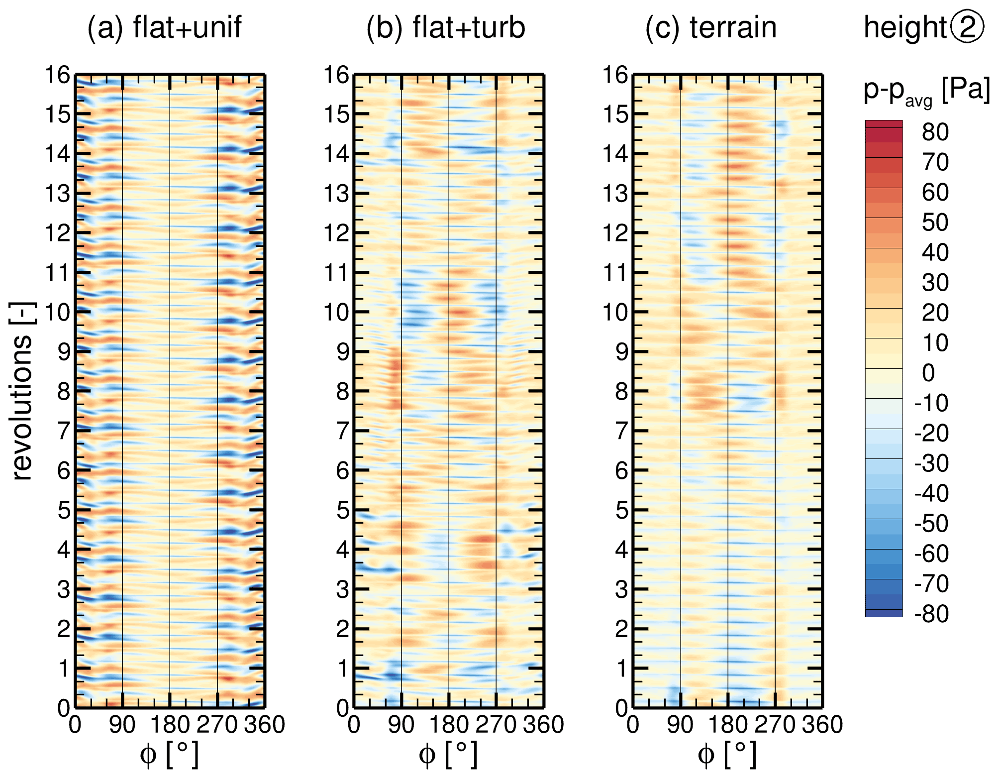
Figure 17 Time series of surface pressure fluctuations p−p_avg on a line around the tower at height (2) for all cases (a)–(c).

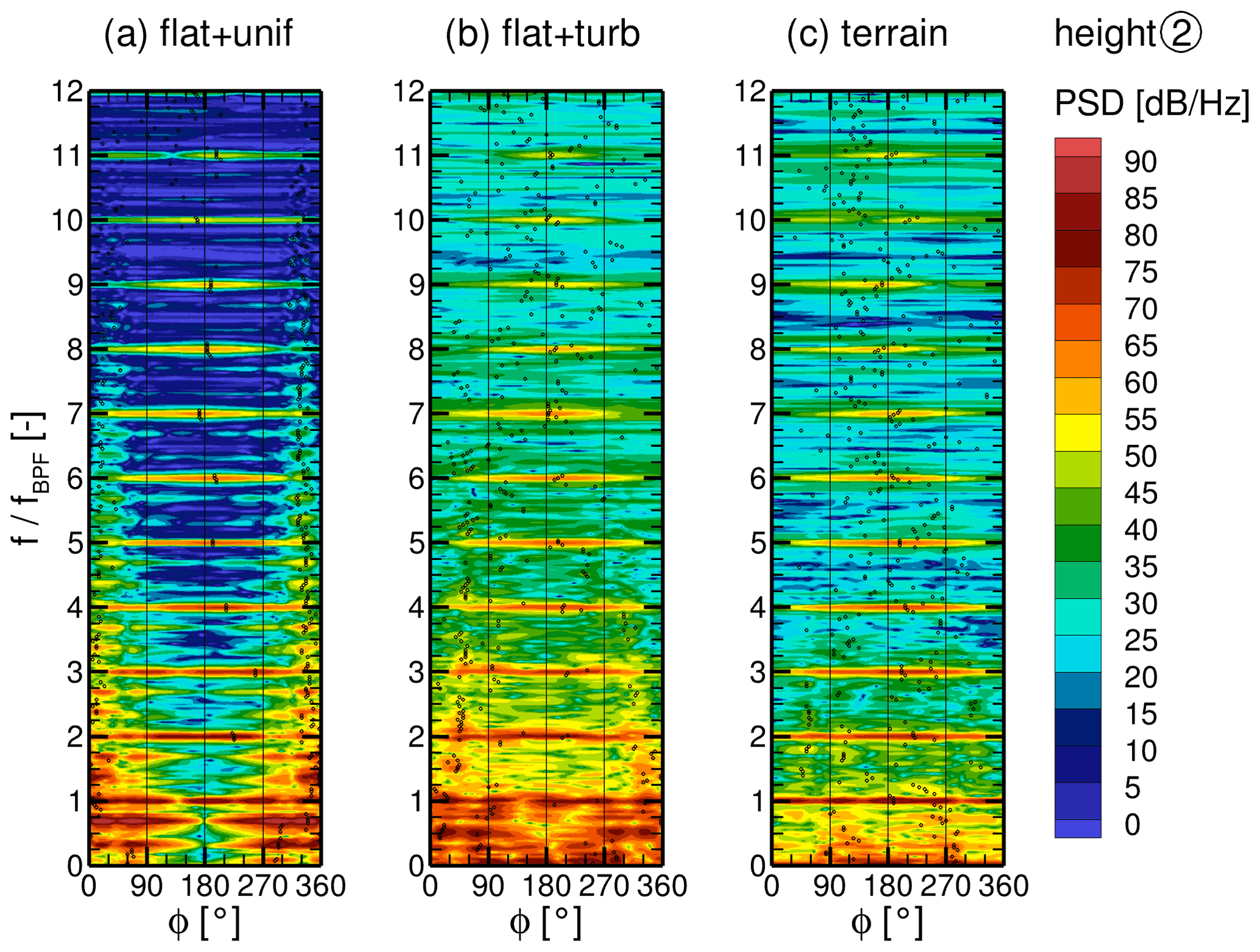
Figure 18 Power spectral density of surface pressure fluctuations on a line around the tower at height (2) for all cases (a)–(c).

Almost all around the tower but particularly at the tower front, pressure fluctuations with the BPF and its harmonics are clearly visible for all cases at height (2) in Fig. 18. They are imposed by the blade tip vortices periodically hitting the tower with the BPF and sweeping over its circumference. Since this periodic interaction is very brief, it acts as an impulse on the tower, and many higher harmonics are visible in the PSD. Looking at Fig. 18a for uniform inflow, it can be seen that the strongest fluctuations still occur with a frequency f=0.59 Hz at the tower sides and back. The amplitude of these pressure fluctuations is even higher than at height (1) since the vertically stretched shed vortices have their highest vorticity in the middle part, where the local tower diameter corresponds to the mean tower diameter. For the flat + turb case, strong pressure fluctuations still occur at the tower sides and back below the BPF associated with vortex shedding, but no discrete shedding frequency can be identified in Fig. 18b. Instead, the inflow turbulence imposes strong broadband pressure fluctuations around the whole tower for frequencies below the BPF. The PSD of the terrain + WT case in Fig. 18c looks remarkably different below the BPF. This is because the terrain flow causes quite different vortex structures at height (2), which is evident when comparing Fig. 15b and c. As described, the inflow turbulence in the terrain flow is much more anisotropic, with ω_z being converted to ω_x, and streamwise vortices cause fewer pressure fluctuations on the tower surface. Moreover, TI in the near field of the turbine is not identical between the flat + turb and the terrain + WT case in this study, with TI being 1.5 percentage points lower in the terrain + WT case. These two factors explain the lower broadband fluctuations in the terrain + WT case.

5.3.3 Surface pressure on tower at height (3)

At height (3) the blade passage causes a very sharp periodic pattern on the side of the descending blade (Φ≈210^∘) for uniform inflow, as visible in Fig. 19a. The turbulent cases also show this periodic pattern (see Fig. 19b and c) but less sharply and superimposed by low-frequency patterns. A less strong periodic pattern on the back of the tower is also visible for all cases, indicating vortex shedding with discrete frequencies again.

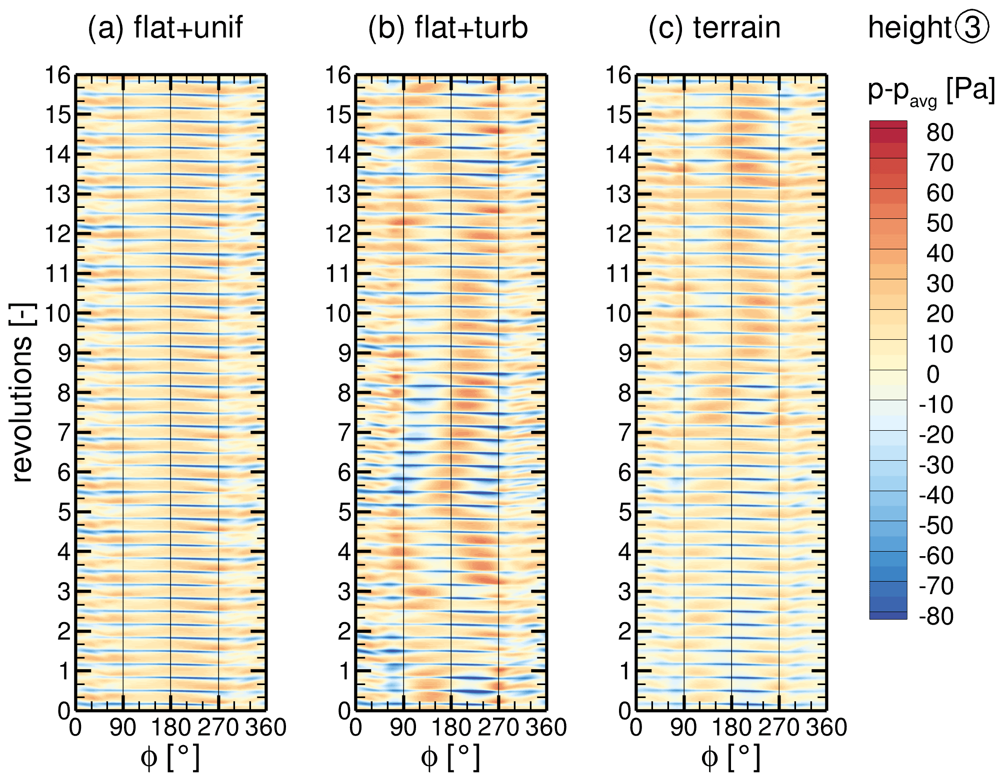
Figure 19 Time series of surface pressure fluctuations p−p_avg on a line around the tower at height (3) for all cases (a)–(c).

Pressure fluctuations with discrete frequencies of the BPF and its harmonics have the highest amplitudes in all cases at height (3), shown in Fig. 20. The fluctuations with the BPF dominate around the whole tower since the reduced pressure on the suction side of the blade extends around the whole tower when the blade passes. The strongest fluctuations with the BPF occur on the side of the descending blade (Φ≈210^∘), marked with black symbols in Fig. 20. This was also found by Klein (2019) and is due to a speed-up of the flow between the tower and the approaching blade, known as the Venturi effect, locally enhancing the pressure reduction. The maxima of the pressure fluctuations with higher harmonics of the BPF drift slightly towards the tower front with increasing frequency. With uniform inflow, even at height (3) where the blades pass, the same vortex-shedding frequency is pronounced at the tower sides and back as at the lower heights, as visible in the PSD in Fig. 20a. This confirms that coherent vortex cells stretch over the entire tower height for uniform inflow, even with the blade wake interaction and a tapered shape of the cylinder. The curved shape of the vortex cells in Fig. 15a is due to the reduced flow velocity behind the blades caused by the blade induction, resulting in a slower downwind propagation of the vortices. The flat + turb case shows the same vortex-shedding frequency, albeit much less pronounced, with a more broadband character of the pressure fluctuations below the BPF. At height (3), the terrain + WT case shows vortex shedding for the first time with a fairly discrete frequency at the tower back, however, at $f=\mathrm{BPF}/\mathrm{2}$. Figure 15c shows the coherent vortices at the upper tower. As mentioned, the horizontal inflow vortices prevent the formation of strong vortex cells extending over the entire tower height, and thus the blade passage impulse is dominant enough to induce periodic vortex shedding on the upper tower, one vortex per blade passage with opposite circulation. This interaction between blade passage and vortex shedding is also described by Gómez et al. (2009), who performed two-dimensional simulations of the blade–tower interaction.

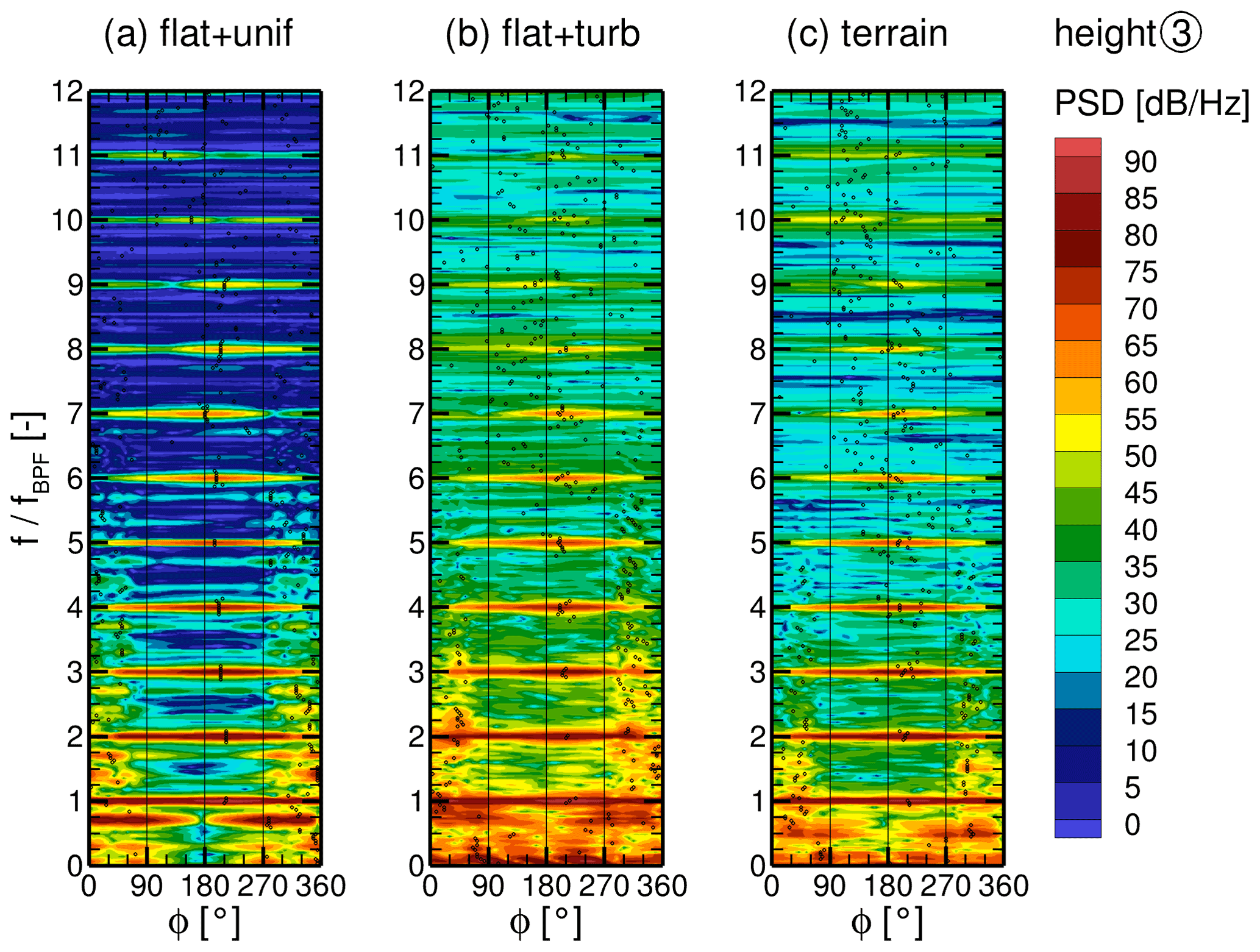
Figure 20 Power spectral density of surface pressure fluctuations on a line around the tower at height (3) for all cases (a)–(c).

Figure 21 shows the maximum amplitude of the pressure fluctuations on the tower with the BPF (f_BPF=0.84 Hz) and its first two higher harmonics (1.69 and 2.53 Hz) and the circumferential position Φ where they occur. Behind the blade passage, above z=35 m, the position and the amplitude of the strongest pressure fluctuations with the BPF and the first two higher harmonics are not significantly altered by the different inflow conditions. This means that the mechanisms of the blade–tower interaction remain unchanged.

Figure 21 Maximum amplitude of the PSD of the surface pressure fluctuations per height and their circumferential position on the tower for the BPF (a) and first (b) and second (c) higher harmonic.

The observations show that the surface pressure fluctuations on the tower are dominated by a superposition of blade-passing effects and tower vortex shedding, as also described by Klein et al. (2018). The inflow characteristic has no significant influence on the fluctuations at the tower in connection with the blade–tower interaction. However, pressure fluctuations due to vortex shedding from the tower are strongly inflow-dependent. It is therefore crucial to take the inflow into account realistically in order to correctly capture the periodicity of the surface pressure fluctuations, which can, for example, drive the occurrence of acoustic low-frequency tonalities.

5.4 Surface pressure on blades

Besides the tower, the blades are the turbine components with the largest surface area. Moreover, they generate most of the aerodynamic loads. Figure 22 shows contour plots of the standard deviation σ of the surface pressure on one blade for all cases. In the plots the blade is unwound and the arc length d from the leading edge (LE) is normalized with the local chord length c, where positive values belong to the suction side (SS) and negative values to the pressure side (PS). Pressure fluctuations are the strongest close to the LE for outer blade radii. Inflow turbulence significantly increases the fluctuations and broadens the region in both the flat + turb and the terrain + WT case. To further look into details, position (4) at 85 % blade radius marked with the red line is chosen. At this radial position the blade generates the highest thrust per metre.

Figure 22 Standard deviation σ of surface pressure p on one blade for all cases (a)–(c).

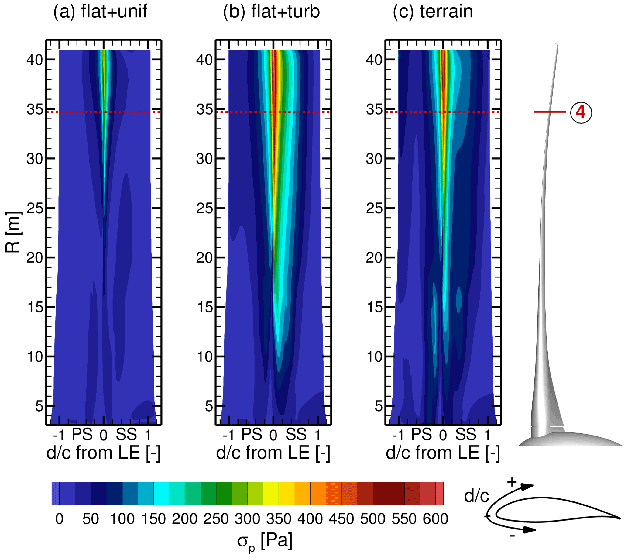
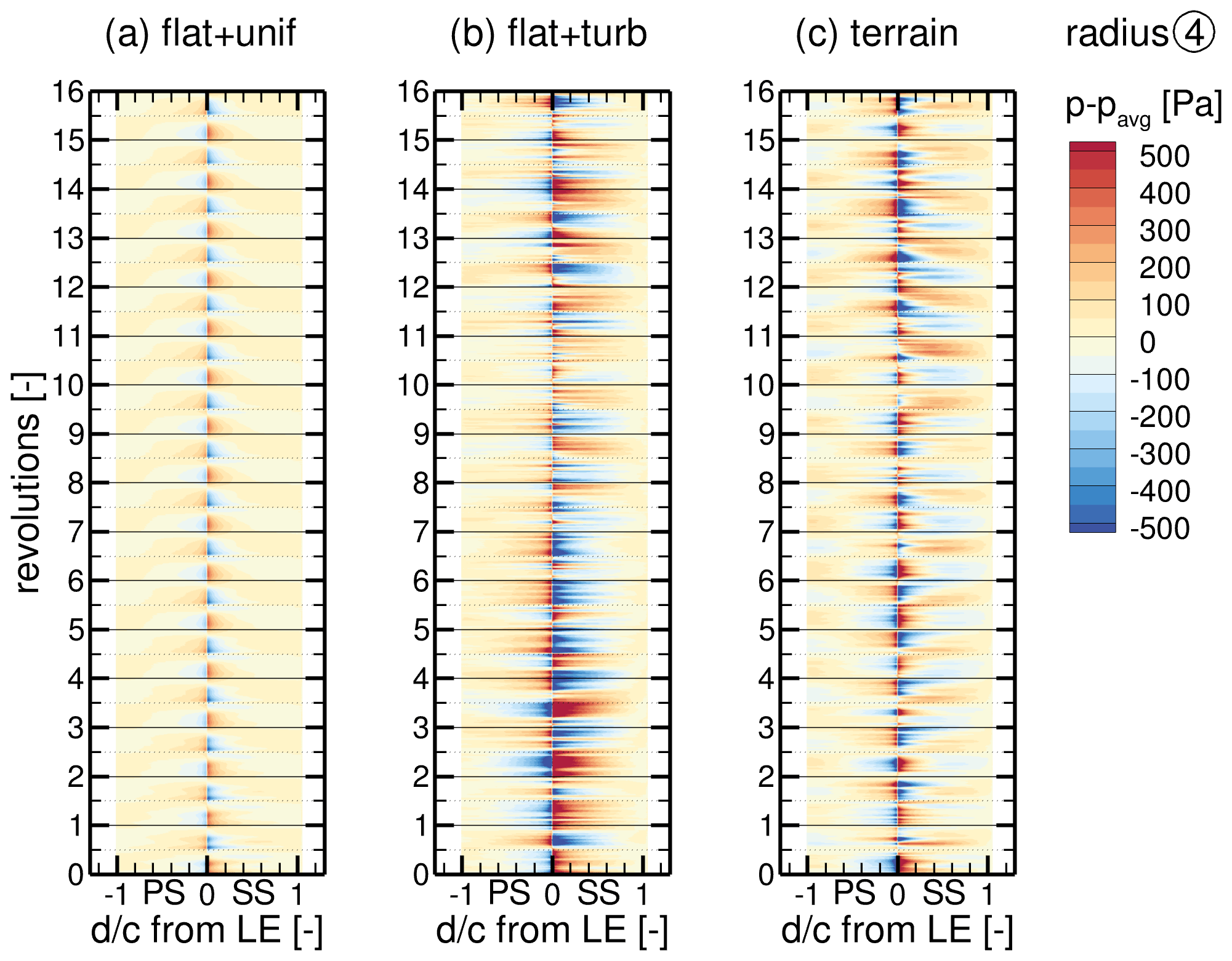
Figure 23 Time series of surface pressure fluctuations p−p_avg along a blade section at the radius (4) for all cases (a)–(c).

The time series of the pressure fluctuations p−p_avg at the blade radius (4) in Fig. 23 show a periodic pattern over the whole circumference with a frequency of once per revolution for the flat + unif case. Towards the LE, the fluctuations are by far the strongest and counter-directed compared to the main part of the airfoil. The reversal of the pressure pattern between the descending (from full to half revolution) and ascending (from half to full revolution) blade is due to the rotor tilt. It causes the effective angle of attack α at radius (4) to be slightly less for the descending blade than for the ascending one (Δα≈0.28^∘). This leads to a small periodic shift of the stagnation point, increasing the pressure on the SS close to LE for the descending blade. In contrast, the effective inflow velocity u_eff at the blade at radius (4) is slightly higher for the descending blade than for the ascending (Δu_eff≈1.7 m s⁻¹). This dominates the global blade load and leads to a lower pressure on the SS and higher one on the PS from ≈0.4c to the trailing edge for the descending blade. These effects also occur for the flat + turb and the terrain + WT cases but are superimposed by the unsteady changes in local flow velocity and direction caused by the inflow turbulence, which generates additional stochastic pressure fluctuations. The unsteady blade deflection (see Fig. 11) additionally changes u_eff and α, resulting in a complex interaction. As on the tower, the flow in the terrain + WT case causes weaker fluctuations compared to the flat + turb case due to the described difference in the inflow turbulence. However, the inclined flow increases α for the ascending blade and reduces it for the descending blade, which amplifies the periodic tilt effect. Furthermore, the slightly vertically sheared inflow (Δu≈0.5 m s⁻¹ over the rotor) in these two cases marginally increases the blade loads in the upper half of the revolution, reducing the pressure on SS and increasing it on PS. For all cases, the tower passage causes a very sharp, impulsive disruption of the pressure pattern (see Fig. 23 at each half revolution) by a sudden reduction in α due to the reduced flow velocity in front of the tower and due to the acceleration of the flow between the blade and tower (Venturi effect). In addition, the higher pressure in the tower dam region is imposed on the blade.

A transformation into the frequency domain, depicted in Fig. 24, confirms the observations. For the flat + unif case at the blade radius (4), peaks are visible at the rotational frequency f_t=0.28 Hz and its multiples. The peak at f_t is caused by a combination of the tilt effect and the blade–tower interaction. The tilt effect is sinusoidal, and therefore the higher harmonics are caused solely by the impulsive blade–tower interaction. The PSD also shows that the pressure fluctuations are not limited to the LE but occur around the whole blade, which is difficult to see in Fig. 23a. Inflow turbulence in the flat + turb and the terrain + WT case dominates at the blade radius (4) above f_t and masks the higher harmonics caused by the blade–tower interaction, resulting in a broadband characteristic of the pressure fluctuations. The most pronounced pressure fluctuations occur in all inflow cases at the rotational frequency. However, the maximum amplitude for that frequency is slightly stronger in the flat + turb case than for uniform inflow due to the vertical wind shear effect, which is also sinusoidal, and is further amplified in the terrain + WT case by the inclination effect.

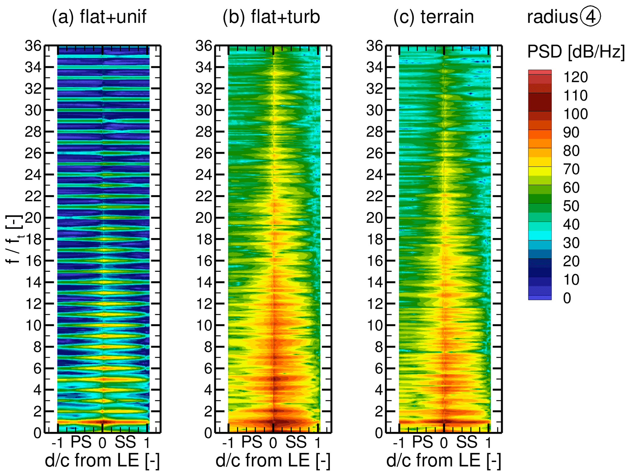
Figure 24 Power spectral density of surface pressure fluctuations on a line around the blade at radius (4) for all cases (a)–(c).

The observations show that the surface pressure fluctuations on the blades are dominated by a combination of the rotor tilt; the blade–tower interaction; and inflow properties, such as turbulence characteristic, vertical wind shear and flow inclination. The changes in the angle of attack and the effective inflow velocity due to the rotor tilt cause the dominant pressure fluctuation at the rotation frequency. The amplitude of this fluctuation is amplified by the vertical wind shear as well as the inclined flow in the terrain. Fluctuations with higher harmonics of this frequency are triggered by the impulsive blade–tower interaction, independent of the inflow. However, the inflow turbulence causes broadband fluctuations, whose strength is directly related to the turbulence intensity, masking these harmonics. Therefore, it is again important to take the inflow into account realistically.

6 Conclusions

In this paper, the impact of turbulent inflow in complex terrain on surface pressure fluctuations on a turbine is investigated numerically using the hybrid RANS–LES flow solver FLOWer. A highly resolved computational setup for a DDES of a WT in the complex terrain at Perdigão, including vegetation, is presented. A new workflow for the generation of site- and situation-specific inflow conditions using a steady-state atmospheric precursor simulation with E-Wind is introduced. The precursor simulation can be calibrated against met mast data, which is exemplified for a measured situation on 10 May 2017. Mean velocity profiles for u, v and w are used directly at the interface, whereas the turbulence field is created using the Mann model. The CFD model described provides numerically stable results of the global terrain flow but shows limitations in simulation of the valley flow and increasing inaccuracy with the distance from the inlet. However, a validation with met mast and lidar data confirms that a site- and situation-specific flow field on the first ridge in Perdigão can be simulated well with the numerical process chain. Both mean velocities and the turbulence spectrum up to 1 Hz are realistically captured at the turbine position, even if the turbulence intensity is somewhat too low due to numerical dissipation. The generic turbine is included in the terrain simulation as a fully meshed structure, and the CFD is coupled to a structural solver. Due to its aero-servo-elastic similarity with commercial turbines, the findings are transferable to the real turbine erected at the site. The characteristics of the turbine wake can be compared with lidar measurements, for example, and are well represented in the simulation.

The detailed simulation of the flow field around the turbine in Perdigão allows a realistic assessment of the impact of the flow in complex terrain on the surface pressure fluctuations on the turbine. Two reference simulations in flat terrain, one with uniform inflow and one with generic inflow turbulence, are performed to identify the terrain impact. It is shown that turbulent inflow alters the frequency and intensity of surface pressure fluctuations caused by vortex shedding at the tower or, more precisely, reduces their periodic pattern. However, the influence of turbulent inflow cannot be generalized. The terrain flow in Perdigão with its streamwise stretched turbulent structures (due to the acceleration at the ridge) causes different vortex shedding at the tower than turbulence in flat terrain. Nevertheless, the dominance of the periodic pressure fluctuations with the BPF and its higher harmonics at the upper tower, caused by the blade–tower interaction, is not noticeably changed by the inflow. At the blade, however, the periodic pressure fluctuations with multiples of the tower passage, which are caused by the impulsive blade–tower interaction, are largely masked by the turbulent inflow. Only the pressure fluctuation with the rotational frequency remains as a discrete frequency under turbulent inflow in the otherwise broadband regime. This is caused by a combination of rotor tilt, vertical wind shear and inclined flow, which again shows how important a realistic consideration of the inflow is.

In future studies, it is planned to post-process the simulation results with a Ffowcs Williams–Hawkings solver to evaluate the low-frequency acoustics. Subsequently, the most important acoustic sources for low-frequency emissions at wind turbines will be localized and compared with the areas found with high surface pressure fluctuations.