How should the lift and drag forces be calculated from 2-D airfoil data for dihedral or coned wind turbine blades?

In the present work, a consistent method for calculating the lift and drag forces from the 2-D airfoil data for the dihedral or coned horizontal-axis wind turbines when using generalized lifting-line methods is described. The generalized lifting-line methods refer to the models that discretize the blade radially into sections and use 2-D airfoil data, for example, lifting-line (LL), actuator line (AL), blade element momentum (BEM) and blade element vortex cylinder (BEVC) methods. A consistent interpretation of classic unsteady 2-D thin airfoil theory results reveals that it is necessary to use both the relative flow information at one point on the chord and the chordwise gradient of the flow direction to correctly determine the 2-D aerodynamic force and moment. Equivalently, the magnitude of the force should be determined by the flow at the three-quarter-chord point, while the force direction should be determined by the flow at the quarter-chord point. However, this aspect is generally overlooked, and most implementations in generalized lifting-line methods use only the flow information at one calculation point per section for simplicity. This simplification will not change the performance prediction of planar rotors but will cause an error when applied to non-planar rotors. In this work this effect is investigated using the special case, where the wind turbine blade has only out-of-plane shapes (blade dihedral) and no in-plane shapes (blade sweep), operating under steady-state conditions with uniform inflow applied perpendicular to the rotor plane. The impact of the effect is investigated by comparing the predictions of the steady-state performance of non-planar rotors from the consistent approach of the LL method with the simplified one-point approaches. The results are verified using blade-geometry-resolving Reynolds-averaged Navier–Stokes (RANS) simulations. The numerical investigations confirmed that the full method complying with the thin airfoil theory is necessary to correctly determine the magnitude and direction of the sectional aerodynamic forces for non-planar rotors. The aerodynamic loads of upwind- and downwind-coned blades that are calculated using the LL method, the BEM method, the BEVC method and the AL method are compared for the simplified and the full method. Results using the full method, including different specific implementation schemes, are shown to agree significantly better with fully resolved RANS than the often used simplified one-point approaches.

1 Introduction

With the scientific and engineering advancements in the design optimization and manufacturing of horizontal-axis wind turbines (HAWTs), modern wind turbine blades are generally more flexible and may have more out-of-plane shapes compared to conventional stiff machines. Also, research on downwind turbines proposed for land-based low-rated-wind applications (Madsen et al., 2020b) and the ultra-light concept (Loth et al., 2012) involve wind turbine rotors with large out-of-plane shapes. Correctly predicting the aerodynamic loads on such non-planar rotors is important for the design optimization and verification of these new concepts. However, it is computationally expensive to use accurate blade-geometry-resolving Navier–Stokes simulations for aerodynamic calculations, especially during the design optimization phase. Instead, low- to mid-fidelity generalized lifting-line aerodynamic models that use 2-D airfoil data provided by Navier–Stokes solvers or wind tunnel measurements are widely used. The models range from the low-fidelity blade element momentum (BEM) method (Madsen et al., 2020a) and blade element vortex cylinder (BEVC) method (Li et al., 2022) to the higher-fidelity lifting-line (LL) method (Phillips and Snyder, 2000) and actuator line (AL) method (Sørensen and Shen, 2002). The advantage of such models is that it is not necessary to directly solve the Navier–Stokes equations for the whole flow domain and resolve the 3-D blade geometry. In addition, the so-called engineering dynamic stall model is usually applied to such generalized lifting-line methods to account for unsteady 2-D effects. However, the dynamic stall name of the model is misleading because the model is also active for non-stalled conditions. Therefore a more proper name for such models is unsteady 2-D airfoil aerodynamic models. For example, in the Beddoes–Leishman-type dynamic stall model (Hansen et al., 2004; Pirrung and Gaunaa, 2018) that is implemented in the HAWC2 code (Larsen and Hansen, 2007; Madsen et al., 2020a), the following effects are modeled: unsteady attached flow, unsteady flow separation (dynamic stall), non-circulatory lift force and the effective pitch rate drag force.

According to unsteady 2-D thin airfoil aerodynamics, it is necessary to use the flow information at both the quarter-chord point and the three-quarter-chord point to correctly determine the magnitude and direction of the lift and drag forces (Bergami and Gaunaa, 2012; Pirrung and Gaunaa, 2018). However, this aspect is generally overlooked and is often not a focus of engineering wind turbine aerodynamic model descriptions (Schepers et al., 2021). For simplicity, most implementations only use the flow information at one calculation point per section. This simplification will not change the performance prediction of planar rotors but will cause an error for non-planar rotors. In this work, a special case is focused on where the blade has only dihedral and no sweep, operating under steady-state conditions with uniform inflow applied perpendicular to the rotor plane. The present work is not intending to propose a new correction since it is already included in a Beddoes–Leishman-type model (Hansen et al., 2004; Pirrung and Gaunaa, 2018). Instead, the focus is to show the importance of this aspect of the unsteady airfoil aerodynamic models even for steady-state computations for any rotor models that use 2-D airfoil data. First, the impact of the one-point simplification is investigated by comparing the results from the LL method using a two-point approach against results following the one-point simplification for non-planar rotors. Furthermore, the results computed from blade-geometry-resolving Reynolds-averaged Navier–Stokes (RANS) simulations are used for comparison. The numerical investigations showed that correctly determining the magnitude and direction of the lift force is important for non-planar rotors. Then, the corrections to the simplified one-point approaches are tested thoroughly. The aerodynamic loads of upwind- and downwind-coned blades are calculated using the LL method, the AL method, the BEM method and the BEVC method, both without and with the correction. In addition, the analytical derivations and numerical results in this work show that the total non-circulatory force is negligible for such steady-state conditions.

The structure of the present work is as follows: the highlights from the unsteady 2-D thin airfoil theory are firstly summarized in Sect. 2. This section also includes the interpretation of these results in terms of what is necessary to be included in generalized lifting-line methods. Then, the non-circulatory forces of a pure dihedral blade under steady-state operating conditions are derived in Sect. 3. Subsequently, the corrections for the generalized lifting-line method that only uses one chordwise calculation point are derived in Sect. 4. Then, different aerodynamic models for the comparison are described in Sect. 6. In Sect. 7, the setup of the numerical tests is described, and the results from different generalized lifting-line methods are compared together with the results from the blade-geometry-resolving RANS solver – both without and with the corrections. Finally, the conclusions and the future work are summarized in Sect. 8.

2 Highlights from unsteady 2-D thin airfoil aerodynamics

Unsteady 2-D thin airfoil theory is of vital importance to correctly model the aerodynamics of wind turbine blades with dihedral using generalized lifting-line methods. The reason is related to the ideas underlying generalized lifting-line methods, which are considered to be the application of perturbation theory (Van Dyke, 1975). The aerodynamics of the full 3-D system is considered to be the combination of an inner and an outer problem. The inner problem is the unsteady 2-D airfoil aerodynamics, and it has a relatively simple 2-D geometry but a locally complex flow (as derived from the Navier–Stokes equations). The outer problem is the 3-D rotor and wake problem that has complex geometry but is assumed to be irrotational flow everywhere except for the bound vortex and the wake that originates from it. The full 3-D aerodynamic problem is approximately solved by solving the two problems together (Johnson, 2013). Analysis using unsteady 2-D thin airfoil theory reveals that this problem is driven by the relative velocities that would have been there if the velocities induced by the 2-D airfoil and its wake were not present. To find this situation for the inner problem, the 3-D flow (including the 3-D induction minus the local 2-D induction), the onset flow and the total motion at each blade section are transformed into the 2-D airfoil section coordinate system, where they are used to solve the inner problem (Li et al., 2020). The results from the inner 2-D problem, which are the sectional forces and the bound circulation, are used as the input for solving the 3-D problem.

In this section, some of the important conclusions and results from unsteady 2-D thin airfoil theory are briefly described. These conclusions will be used to derive the non-circulatory forces in Sect. 3 and are important to determine the magnitude and direction of the lift force in Sect. 4. A detailed derivation of 2-D unsteady thin airfoil theory, also including the analysis of details behind a consistent evaluation of unsteady drag, is shown in Gaunaa (2010). This previous work also considers the effect of a deformable or morphable camber line. But if the camber line shape is not changing over time, the classical steady and unsteady 2-D thin airfoil results are recovered. It is seen from the results of the analysis that the local pressure difference anywhere on the thin airfoil is determined from the undisturbed relative local flow velocities and their time history over the whole airfoil chord length. It does not matter how the relative flow velocities (and their time history) arise; if two situations have the same “input”, the resulting pressure differences over the airfoil will be the same. This information is crucial for the interpretation of the thin airfoil results in the more general case, where the thin airfoil framework results are to be used “inside” the framework of the general lifting-line methods. More specifically, it is the magnitude of the relative wind speed and the local normal flow velocity (the component of the relative flow velocity in the direction locally normal to the chord line) that drives the solution of the local pressure differences and thereby also the integral airfoil section forces.

For the present work, the simplest representation of an uncambered airfoil, a flat plate, with a chord length of c=2b that is placed in a uniform flow with the free-stream velocity of V is considered. The geometric flow angle θ is the angle between the flow and the flat plate. The airfoil motion is described by a heaving motion $\dot{y}$ (positive upward, perpendicular to the incoming flow), a pitching motion $\dot{\mathit{\theta }}$ about the axis at ξ=ab (positive nose-up) and a horizontal motion of $\dot{x}$ (positive direction downwind). A sketch of the coordinate system and the geometry of a flat plate to derive the unsteady 2-D thin airfoil theory is shown in Fig. 1.

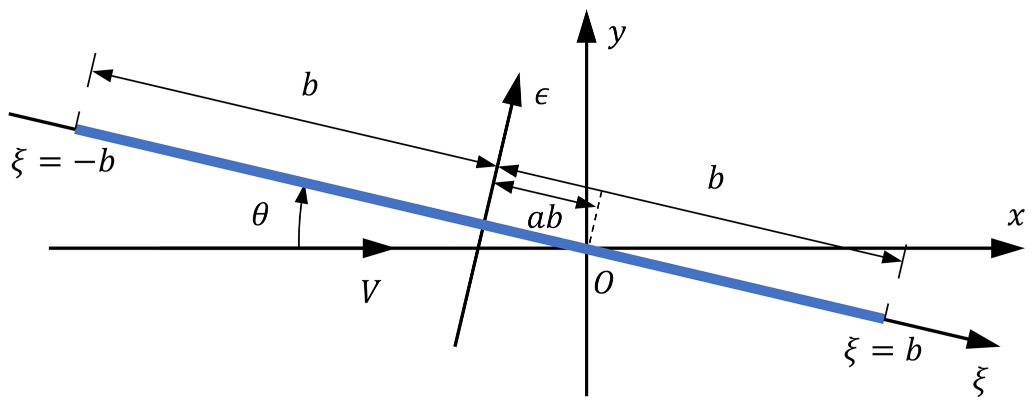
Figure 1 Definitions of the coordinate system and positive directions used in the derivations of the unsteady 2-D thin airfoil theory.

Essentially, the fundamental output from the thin airfoil analysis is the local unsteady pressure difference over the airfoil and the leading edge suction force. At the leading edge of an airfoil, there is generally a low pressure because the air is accelerated around the relatively small leading edge radius. In thin airfoil theory the airfoil thickness, and along with it the leading edge radius, tends to zero. This results in the pressure tending to minus infinity at the leading edge¹, which has an effective area tending to zero. The leading edge suction force can be considered the limit of the pressure acting on the leading edge area as the leading edge radius tends to zero. It acts in the airfoil tangential (−ξ) direction, pointing from the trailing edge to the leading edge. The pressure difference over the airfoil in the flat-airfoil case acts locally normal to the airfoil surface, and therefore in this flat-airfoil case only in the normal (ϵ) direction. Therefore, the integral forces on the airfoil consist of the contributions from the normal force N and the tangential force T, which have the relationship of $\left|T\right|\ll \left|N\right|$. The force components usually used in generalized lifting-line methods are lift and drag, which are defined relative to a local flow direction and not relative to the orientation of the airfoil. The corresponding lift and drag forces are the projection of the normal and tangential force according to the reference direction, which is explained in the following and illustrated in Fig. 2.

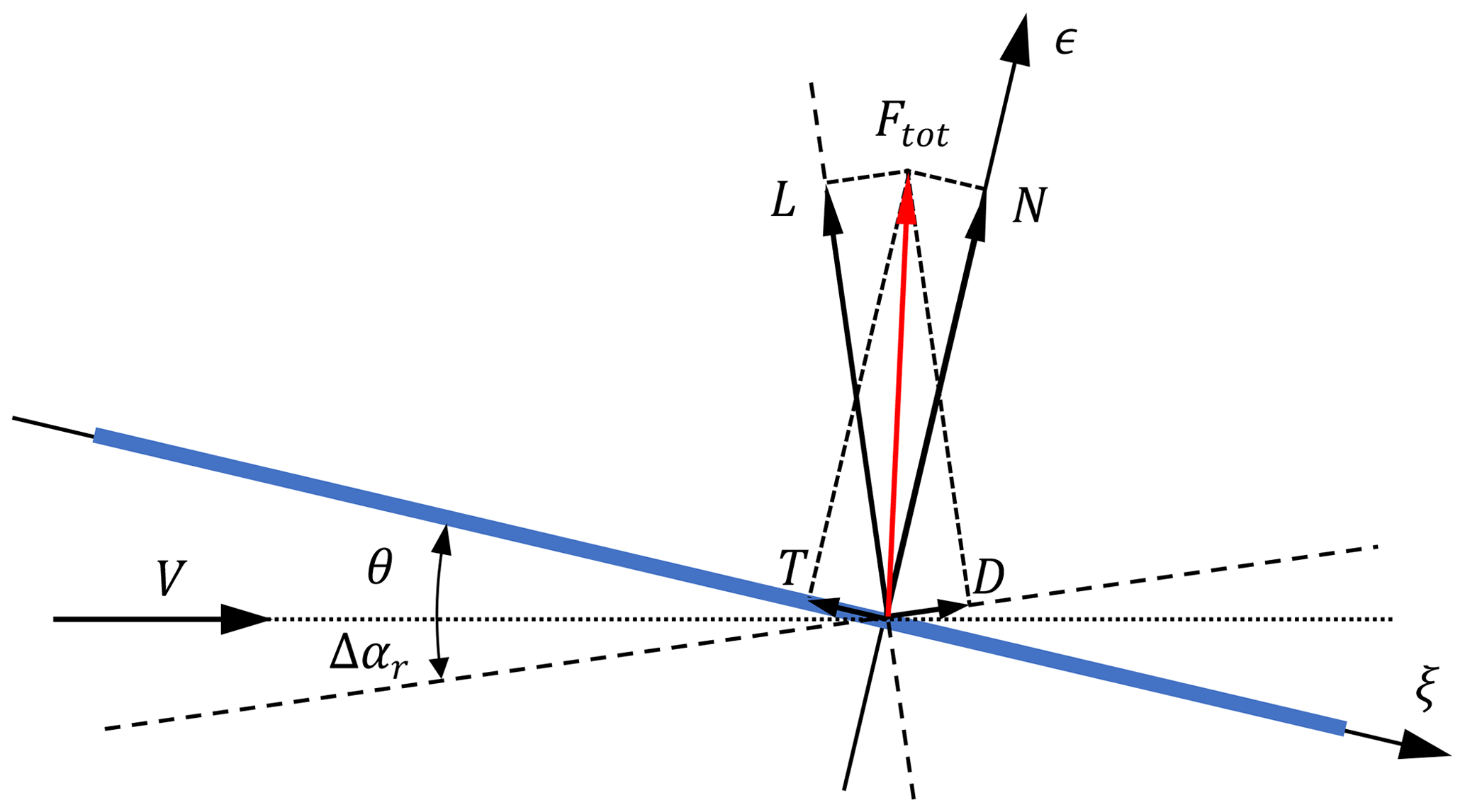
Figure 2 Projection of the normal and tangential forces (N and T) to the lift and drag forces (L and D) that are defined according to a flow direction that has an angle of Δα_r from the geometric flow direction. The choice of the reference direction, which consequently defines lift and drag, could be arbitrary as long as the same total force F_tot is obtained.

2.1 The lift force magnitude

The lift force that is defined according to the effective flow direction that deviates by an angle of Δα_r from the geometric flow direction as shown in Fig. 2 can be derived by projecting the normal and tangential forces.

$$\begin{array}{}\text{(1)}& L=N\cos (\mathit{\theta }+\mathrm{\Delta }{\mathit{\alpha }}_{\mathrm{r}})-T\sin (\mathit{\theta }+\mathrm{\Delta }{\mathit{\alpha }}_{\mathrm{r}})\end{array}$$

In the equation above, Δα_r is the contribution from the airfoil motion to the angle of attack, which is shown in more detail in Sect. 2.2. In the derivation of thin airfoil theory, it is assumed that the angles of attack are small. In addition, the relative velocities due to airfoil motion are significantly smaller than the onset flow velocity. Under these assumptions the detailed definition of the angle of attack is not important for the evaluation of the lift force because $|\mathit{\theta }+\mathrm{\Delta }{\mathit{\alpha }}_{\mathrm{r}}|\ll \mathrm{1}$, which together with $\left|T\right|\ll \left|N\right|$ inserted into Eq. (1) leads to

$$\begin{array}{}\text{(2)}& L\approx N.\end{array}$$

Using the expression for the normal force N derived in Gaunaa (2010) the lift force for the oscillatory case is obtained².

$$\begin{array}{}\text{(3)}& \begin{array}{rl}L& =\underset{L^{\mathrm{C}}=L^{\mathrm{QS}}C\left(k\right)}{\underbrace{\mathrm{2}\mathit{\pi }\mathit{\rho }b(V-\dot{x})\left[(V-\dot{x})\mathit{\theta }-\dot{y}+\left({\displaystyle \frac{\mathrm{1}}{\mathrm{2}}}-a\right)b\dot{\mathit{\theta }}\right]C\left(k\right)}}\\ & +\underset{L^{\mathrm{NC}}}{\underbrace{\mathit{\pi }\mathit{\rho }{b}^{\mathrm{2}}\left[(V-\dot{x})\dot{\mathit{\theta }}-\ddot{x}\mathit{\theta }-\ddot{y}-ab\ddot{\mathit{\theta }}\right]}},\end{array}\end{array}$$

where C(k) is Theodorsen's lift deficiency function (Theodorsen, 1935), and k is the reduced frequency:

$$\begin{array}{}\text{(4)}& k=\mathrm{\Omega }b/V.\end{array}$$

The first term of the lift force is the circulatory lift force, L^C, which through Theodorsen's lift deficiency function takes the unsteady 2-D shed wake into account if temporal variations in the quasi-steady lift, L^QS, are present. If L^QS is constant, then C(k)=1. The second lift term, L^NC, is the non-circulatory lift force, which always acts instantaneously without any time lag.

2.1.1 Circulatory lift

To have a better understanding of the circulatory lift equation in Eq. (3) in the context of the generalized lifting-line methods, it is convenient to express it as an explicit function of the angle of attack. To determine the angle of attack more precisely, it is necessary to firstly consider how it is defined. The component of the relative flow velocity in the direction perpendicular to the airfoil (ϵ direction) is usually termed the upwash. The upwash at a chordwise position with the coordinate of ξ is

$$\begin{array}{}\text{(5)}& w=(V-\dot{x})\mathit{\theta }-\dot{y}+(\mathit{\xi }-ab)\dot{\mathit{\theta }}.\end{array}$$

By setting $\mathit{\xi }=\frac{\mathrm{1}}{\mathrm{2}}b$, the upwash at the three-quarter-chord point is obtained.

$$\begin{array}{}\text{(6)}& w_{\mathrm{3}/\mathrm{4}}=(V-\dot{x})\mathit{\theta }-\dot{y}+({\displaystyle \frac{\mathrm{1}}{\mathrm{2}}}-a)b\dot{\mathit{\theta }}\end{array}$$

Since an angle of attack is defined as the angle between a flow direction and the chord line, in this case using the small-angle approximation, ${\mathit{\alpha }}_{\mathrm{3}/\mathrm{4}}\approx w_{\mathrm{3}/\mathrm{4}}/(V-\dot{x})$, the circulatory lift in Eq. (3) can be written as

$$\begin{array}{}\text{(7)}& L^{\mathrm{C}}=\mathrm{2}\mathit{\pi }\mathit{\rho }b(V-\dot{x})w_{\mathrm{3}/\mathrm{4}}C\left(k\right)={\displaystyle \frac{\mathrm{1}}{\mathrm{2}}}\mathit{\rho }(V-\dot{x}{)}^{\mathrm{2}}c\mathrm{2}\mathit{\pi }{\mathit{\alpha }}_{\mathrm{3}/\mathrm{4}}C(k).\end{array}$$

This means the magnitude of the circulatory lift is correctly determined by using the angle of attack at the three-quarter-chord point. After furthermore noting that under the thin airfoil approximations, the relative wind speed is equal to $(V-\dot{x})$, the circulatory lift expression can be finally written in terms of the 2-D lift airfoil data as

$$\begin{array}{}\text{(8)}& L^C={\displaystyle \frac{\mathrm{1}}{\mathrm{2}}}\mathit{\rho }{V}_{\mathrm{rel}}^{\mathrm{2}}c{C}_{\mathrm{L}}^{\mathrm{QS}}\left({\mathit{\alpha }}_{\mathrm{3}/\mathrm{4}}\right)C\left(k\right).\end{array}$$

2.1.2 Non-circulatory lift

The non-circulatory lift in Eq. (3) is summarized as follows.

$$\begin{array}{}\text{(9)}& L^{\mathrm{NC}}=\mathit{\pi }\mathit{\rho }{b}^{\mathrm{2}}\left[\left(V-\dot{x}\right)\dot{\mathit{\theta }}-\ddot{x}\mathit{\theta }-\ddot{y}-ab\ddot{\mathit{\theta }}\right]\end{array}$$

According to Eq. (9), the pitch rate of the airfoil $\dot{\mathit{\theta }}$, the pitching acceleration of the airfoil $\ddot{\mathit{\theta }}$, the heave acceleration of the airfoil $\ddot{y}$ perpendicular to the flow and the streamwise acceleration of the airfoil $\ddot{x}$ will all contribute to the non-circulatory lift.

2.2 Lift force direction and 2-D drag

One of the key conclusions that can be drawn from a full unsteady 2-D thin airfoil theory analysis regarding application in generalized lifting-line methods is usually overlooked: a consistent definition of the direction with which lift and drag forces are defined. Even though the details may at first glance seem overwhelmingly focused on unimportant details, the effect of skipping these details can in some cases lead to completely unphysical behaviors. This is shown by an example in Appendix B.

As stated previously, the local angles of attack observed at different locations on the chord line differ from each other in the general unsteady case due to the pitching or torsional motion of the blade. By use of Eq. (5), the angle of attack observed in the chordwise position ξ can be determined.

$$\begin{array}{}\text{(10)}& \mathit{\alpha }\left(\mathit{\xi }\right)={\displaystyle \frac{w\left(\mathit{\xi }\right)}{(V-\dot{x})}}={\displaystyle \frac{(V-\dot{x})\mathit{\theta }-\dot{y}+(\mathit{\xi }-ab)\dot{\mathit{\theta }}}{(V-\dot{x})}}\end{array}$$

The result of the analysis will reveal that there is a special significance of the quarter-chord point, $\mathit{\xi }=-\frac{\mathrm{1}}{\mathrm{2}}b$, so the complexity of performing a more general analysis is skipped, and we consider directly the angle of attack at the quarter-chord point.

$$\begin{array}{}\text{(11)}& {\mathit{\alpha }}_{\mathrm{1}/\mathrm{4}}={\displaystyle \frac{w\left(\mathit{\xi }=-\frac{\mathrm{1}}{\mathrm{2}}b\right)}{(V-\dot{x})}}={\mathit{\alpha }}_{\mathrm{3}/\mathrm{4}}-{\displaystyle \frac{b\dot{\mathit{\theta }}}{(V-\dot{x})}}\end{array}$$

Using this angle of attack as the reference with which the drag force is defined, which means applying ${\mathit{\alpha }}_{\mathrm{1}/\mathrm{4}}=\mathit{\theta }+\mathrm{\Delta }{\mathit{\alpha }}_{\mathrm{r}}$ in Fig. 2 together with the usual thin airfoil small-angle approximation, the corresponding drag force is

$$\begin{array}{}\text{(12)}& D_{\mathrm{1}/\mathrm{4}}=N\sin {\mathit{\alpha }}_{\mathrm{1}/\mathrm{4}}-T\cos {\mathit{\alpha }}_{\mathrm{1}/\mathrm{4}}\approx N{\mathit{\alpha }}_{\mathrm{1}/\mathrm{4}}-T\end{array}$$

The tangential force, which in the uncambered airfoil case stems entirely from the leading edge suction force, is given by Gaunaa (2010) for the flat-airfoil case as

$$\begin{array}{}\text{(13)}& T={\displaystyle \frac{\mathit{\pi }}{\mathrm{2}}}\mathit{\rho }b{\left(\mathrm{2}(V-\dot{x}){\mathit{\alpha }}_{\mathrm{3}/\mathrm{4}}C\left(k\right)-b\dot{\mathit{\theta }}\right)}^{\mathrm{2}}.\end{array}$$

Inserting the results from Eqs. (2), (3), (11) and (13) into Eq. (12), it can be shown that

$$\begin{array}{}\text{(14)}& D_{\mathrm{1}/\mathrm{4}}=\underset{D_i}{\underbrace{-L^{\mathrm{C}}\mathrm{\Delta }{\mathit{\alpha }}_i}}+\underset{D^{\mathrm{NC}}}{\underbrace{L^{\mathrm{NC}}{\mathit{\alpha }}_{\mathrm{1}/\mathrm{4}}}}\underset{D_{\mathrm{pitchrate}}}{\underbrace{-{\displaystyle \frac{\mathrm{1}}{\mathrm{2}}}\mathit{\pi }\mathit{\rho }{b}^{\mathrm{3}}{\dot{\mathit{\theta }}}^{\mathrm{2}}}},\end{array}$$

where Δα_i can be considered to be the effective induced angle of attack due to the unsteady 2-D wake

$$\begin{array}{}\text{(15)}& \mathrm{\Delta }{\mathit{\alpha }}_i={\displaystyle \frac{L^{\mathrm{C}}-L^{\mathrm{QS}}}{\mathrm{2}\mathit{\pi }\mathit{\rho }b(V-\dot{x}{)}^{\mathrm{2}}}}.\end{array}$$

Each component of the drag force in Eq. (14) is described briefly below.

2.2.1 Shed-wake-induced drag

The term D_i in Eq. (14) is the induced drag force, which is an effective drag that originates from the changed direction of the circulatory lift force due to the induced velocity from the shed vorticity in the wake after an unsteady airfoil. For steady-state conditions, the bound circulation strength does not change with time, which means that there is no shed-wake-induced drag force. This is in agreement with the term in Eq. (15) under the condition of L^C=L^QC, which results in zero induced unsteady 2-D drag.

2.2.2 Non-circulatory drag

In Eq. (14), the drag component of D^NC is the effective drag force due to the projection of the non-circulatory lift L^NC. It is seen that the direction of the non-circulatory force is perpendicular to the chord.

2.2.3 Drag due to pitch rate

The last term D_pitchrate of the drag force is due to the pitch rate and is in some sense a drag equivalent to the non-circulatory lift term due to the pitch rate, $\mathit{\pi }\mathit{\rho }{b}^{\mathrm{2}}(V-\dot{x})\dot{\mathit{\theta }}$. When the airfoil has a pitching motion, there will be a linear variation in upwash along the chord, which results in this drag term. The magnitude of this drag component is proportional to the square of the pitch rate $\dot{\mathit{\theta }}$. For the airfoils with low to moderate reduced frequency, this term is negligible.

2.2.4 Using a different reference direction for drag

In analogy with Eq. (12), the drag defined from the angle of attack at the three-quarter-chord point turns out to be

$$\begin{array}{}\text{(16)}& \begin{array}{rl}{D}_{\mathrm{3}/\mathrm{4}}& =N\sin {\mathit{\alpha }}_{\mathrm{3}/\mathrm{4}}-T\cos {\mathit{\alpha }}_{\mathrm{3}/\mathrm{4}}\approx N{\mathit{\alpha }}_{\mathrm{3}/\mathrm{4}}-T=D_{\mathrm{1}/\mathrm{4}}\\ & +L{\displaystyle \frac{b\dot{\mathit{\theta }}}{(V-\dot{x})}}.\end{array}\end{array}$$

For cases with non-negligible pitch rate, the differences in the two different drag values, in Eqs. (14) and (16), can be quite substantial. In some cases, it is even possible that the contribution from the last term in the three-quarter-chord reference-based drag can have a steady negative value, which is counterintuitive. For this reason, it is suggested to use the quarter-chord reference direction definition of the drag coefficient in aeroelastic codes. Note that both situations reflect the same physics and also exactly the same total force magnitude and direction. As long as the reference directions are handled correctly both methods give exactly the same correct result. An example is illustrated with a vertical-axis wind turbine (VAWT) operating in zero onset flow in Appendix B.

These important details about the drag are generally overlooked but are important for the performance prediction of dihedral blades, which is investigated in Sect. 4. It should be emphasized that the considerations in this section are derived from the thin airfoil theory, which does not include the effects of steady 2-D profile drag. This extra drag component from the 2-D airfoil polars has to be added to the contributions from the thin airfoil theory in the generalized lifting-line methods.

2.3 Application of thin airfoil aerodynamics in an aeroelastic context

When applying these results from thin airfoil aerodynamics in an aeroelastic model, it might seem as if it needs to be carefully considered whether components of the relative motion of the airfoil with respect to the surrounding air are due to a change in flow speed (e.g., due to a gust) or due to a motion of the airfoil itself.

To avoid this issue, it is chosen in Hansen et al. (2004) to treat gusts as an instantaneous change in wind speed everywhere around the airfoil and then apply the Wagner function to approximate the unsteadiness due to the 2-D wake induction. With this assumption, changes in airfoil motion in the chordwise direction or in the direction perpendicular to the chord have the exact same effect as gusts in those directions: changing the relative flow speed and angle of attack seen by the airfoil. The error due to the assumption of the gust affecting the complete flow field instantaneously is investigated in Buhl et al. (2005). For an oscillating inflow at a reduced frequency of 0.25 (corresponding to a frequency of 5.6 Hz at an airfoil section with 1 m chord and a relative speed of 70 m s⁻¹), this simplification causes a relative error in the force amplitude of roughly 3 % and a phase error of below 0.3^∘. Due to this assumption it is not necessary to differentiate if the relative velocity or angle of attack experienced at the airfoil is due to airfoil motion (including the motion due to rotor rotation) or the incoming wind.

The only airfoil motion that remains to be treated individually is the torsion rate of the airfoil, which does not cause a constant change in velocity along the chord (like the gusts with the assumption described above or a translation of the airfoil). Instead, the torsion rate causes a velocity that varies linearly with the position on the chord. The torsion rate is then the total rotation rate of the airfoil section about an axis perpendicular to the cross-section, including influences from rotor rotation, blade torsion and any movement of the substructure that contributes to this rotation.

3 Non-circulatory lift of a pure dihedral blade

In this section, the focus is on the special case that the rotor is non-planar, and the blades have no sweep. For this special case, the blade pitch angle is set to be zero since pitching the blade will result in blade in-plane geometries. The blades are operating at steady-state, with uniform inflow applied perpendicular to the rotor plane, and the rotor has zero tilt and no yaw error. The influence of the non-circulatory lift on such a pure dihedral blade is derived analytically in this section.

3.1 Coordinate system and transformation matrix

Following the conventions in the HAWC2 code, the main axis of the blade is chosen to be the half-chord line. The airfoils are aligned perpendicular to this main axis. Since it is necessary to perform the projection of the 3-D motion of the blade section into the 2-D airfoil section for the analysis, it is convenient to introduce different coordinate systems and the corresponding transformation matrices between them. Three coordinate systems, which are the blade coordinate system, the sectional coordinate system and the local flow coordinate system are used in the present work. The three different coordinate systems and the relationship among them are illustrated in Fig. 3.

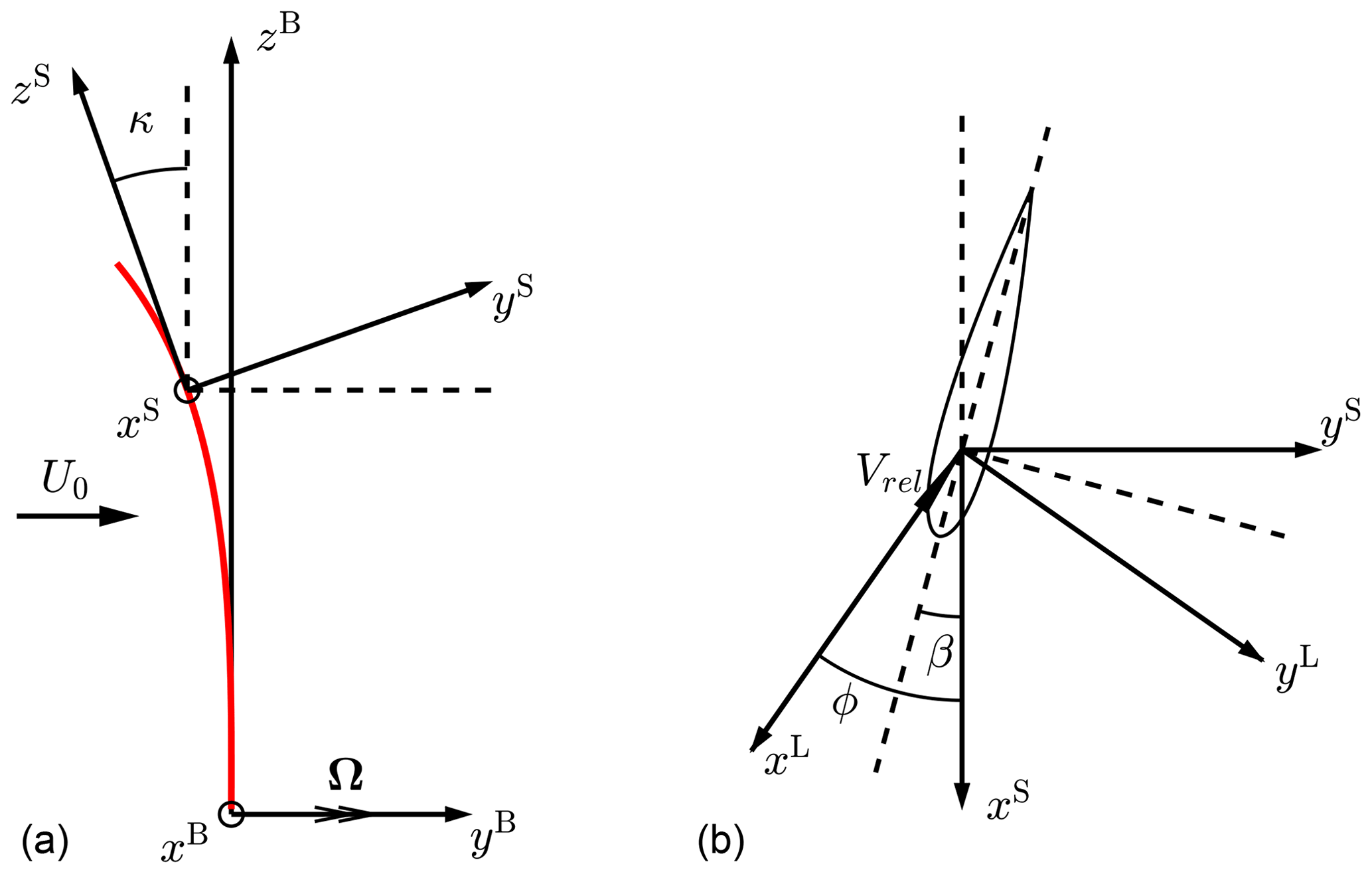
Figure 3 Illustration of the blade coordinate system B, the sectional coordinate system S and the local flow coordinate system L for a blade with only dihedral and no sweep. The sectional coordinate system is the blade coordinate system rotated around its x^B axis with the local dihedral angle κ, as shown in the left panel. The flow angle in the sectional coordinate system is ϕ. The local flow coordinate system is the sectional coordinate system rotated around its z^S axis with −ϕ, as shown in the right panel.

It is assumed that the turbine has three identical blades. The blade coordinate system is a rotating system following a blade that is chosen for reference. For the blade coordinate system, the y^B axis follows the free-stream direction and is defined as the axial direction. The z^B axis is the “radial” direction and is positive in the direction of increasing radius. The x^B axis is defined as the tangential direction. It is normal to both the y^B axis and z^B axis, and its direction is defined so that a right-handed system is found. The sectional coordinate system is the blade coordinate system rotated around the x^B axis with the local dihedral angle κ so that the z^S axis is tangent to the main axis of this section and is positive in the direction of increasing curved blade length. The local flow coordinate system is the sectional coordinate system rotated around the −z^S axis with the local flow angle ϕ so that the x^L axis is pointing to the local flow direction. There is only one blade coordinate system for the whole blade, and each section has its own sectional coordinate system and local flow coordinate system.

The connection between the 3-D flow and motion projected into the local flow system and the unsteady 2-D airfoil theory introduced in Sect. 2 is briefly described to shed light on the connections between the 3-D problem and the 2-D problem. The total 3-D flow velocity relative to the blade V_3−D consists of the inflow; the total motion of the blade section; and the 3-D wake induction minus the 2-D bound vortex induction (Li et al., 2020), which is projected into the local flow coordinate system. The key principle in connecting the 3-D system to the inner 2-D airfoil theory framework is that the relative inflow conditions (and their time derivative) at all locations along the chord should be matched. This assures that the loads from the inner 2-D framework match the 3-D aerodynamic situation. Consider for example the effective pitching motion in Sect. 3.3. The projection of V_3−D into the local flow coordinate system is V_rel, which corresponds to $(V-\dot{x})$ in the 2-D theory in Eq. (3). The x^L and y^L axis correspond to negative x axis and positive y axis of the 2-D system as in Fig. 1, respectively. For the steady-state case of a pure dihedral blade that is shown in Fig. 3, the mounting point is the half-chord point, which corresponds to a=0 in Fig. 1; the geometric flow angle θ in the 2-D theory corresponds to the value of (ϕ−β) as seen in the sectional coordinate system in Fig. 3; and the total 3-D motion of the section is only due to the rotation of the rotor, which has an angular velocity of Ω and the corresponding centrifugal acceleration.

For a blade section, the position vector p, the angular velocity vector Ω and the centrifugal acceleration vector a in the blade coordinate system B are as follows:

$$\begin{array}{}\text{(17)}& {\mathit{p}}^{\mathrm{B}}=\left(\begin{array}{c}\mathrm{0}\\ y\\ z\end{array}\right),{\mathbf{\Omega }}^{\mathrm{B}}=\left(\begin{array}{c}\mathrm{0}\\ \mathrm{\Omega }\\ \mathrm{0}\end{array}\right),{\mathit{a}}^{\mathrm{B}}=\left(\begin{array}{c}\mathrm{0}\\ \mathrm{0}\\ -{\mathrm{\Omega }}^{\mathrm{2}}z\end{array}\right).\end{array}$$

The dihedral angle κ is defined using the main-axis geometry in the blade coordinate system and is defined to be positive when the blade is tilting upwind.

$$\begin{array}{}\text{(18)}& \mathit{\kappa }=-\arctan {\displaystyle \frac{\mathrm{d}y}{\mathrm{d}z}}\end{array}$$

The transformation matrix from the blade coordinate system B to the sectional coordinate system S is determined by the local dihedral angle κ.

$$\begin{array}{}\text{(19)}& {\mathbf{T}}_{\mathrm{B}\to \mathrm{S}}=\left[\begin{array}{ccc}\mathrm{1}& \mathrm{0}& \mathrm{0}\\ \mathrm{0}& \cos \mathit{\kappa }& \sin \mathit{\kappa }\\ \mathrm{0}& -\sin \mathit{\kappa }& \cos \mathit{\kappa }\end{array}\right]\end{array}$$

For the airfoil section with the local flow angle of ϕ, the transformation matrix from the sectional coordinate system S to the local flow coordinate system L is

$$\begin{array}{}\text{(20)}& {\mathbf{T}}_{\mathrm{S}\to \mathrm{L}}=\left[\begin{array}{ccc}\cos \mathit{\varphi }& -\sin \mathit{\varphi }& \mathrm{0}\\ \sin \mathit{\varphi }& \cos \mathit{\varphi }& \mathrm{0}\\ \mathrm{0}& \mathrm{0}& \mathrm{1}\end{array}\right].\end{array}$$

For a given transformation matrix, the reverse transformation matrix is equal to its transposed matrix. This is because the transformation matrices are orthonormal.

3.2 Mid-chord acceleration

For the pure dihedral blade, the projection of the centrifugal acceleration from the blade coordinate system into the local flow coordinate system is obtained using the transformation matrices in Eqs. (19) and (20).

$$\begin{array}{}\text{(21)}& {\mathit{a}}^{\mathrm{L}}={\mathbf{T}}_{\mathrm{S}\to \mathrm{L}}{\mathbf{T}}_{\mathrm{B}\to \mathrm{S}}{\mathit{a}}^{\mathrm{B}}=\left(\begin{array}{c}{\mathrm{\Omega }}^{\mathrm{2}}z\sin \mathit{\kappa }\sin \mathit{\varphi }\\ -{\mathrm{\Omega }}^{\mathrm{2}}z\sin \mathit{\kappa }\cos \mathit{\varphi }\\ -{\mathrm{\Omega }}^{\mathrm{2}}z\cos \mathit{\kappa }\end{array}\right)\end{array}$$

According to Eq. (21) the mid-chord point of the airfoil section will have an effective acceleration relative to the local flow direction. The effective mid-chord heave acceleration is the y component of a^L, and the corresponding non-circulatory lift is obtained using Eq. (9).

$$\begin{array}{}\text{(22)}& L_{\mathrm{heav}}^{\mathrm{NC}}=-\mathit{\pi }\mathit{\rho }{b}^{\mathrm{2}}{a}_y^{\mathrm{L}}=\mathit{\pi }\mathit{\rho }{b}^{\mathrm{2}}{\mathrm{\Omega }}^{\mathrm{2}}z\sin \mathit{\kappa }\cos \mathit{\varphi }\end{array}$$

There is also an effective streamwise acceleration that is equal to the negative value of $a_x^{\mathrm{L}}$, and the corresponding non-circulatory lift is derived using Eq. (9).

$$\begin{array}{}\text{(23)}& \begin{array}{rl}{L}_{\mathrm{stream}}^{\mathrm{NC}}& =-\mathit{\pi }\mathit{\rho }{b}^{\mathrm{2}}(\mathit{\varphi }-\mathit{\beta }){\mathrm{\Omega }}^{\mathrm{2}}z\sin \mathit{\kappa }\sin \mathit{\varphi }\\ & =L_{\mathrm{heav}}^{\mathrm{NC}}(\mathit{\varphi }-\mathit{\beta })\tan \mathit{\varphi }\end{array}\end{array}$$

Since the term (ϕ−β) is small, the total non-circulatory lift due to the projection of the centrifugal acceleration is then³

$$\begin{array}{}\text{(24)}& L_{\mathrm{acc}}^{\mathrm{NC}}=L_{\mathrm{heav}}^{\mathrm{NC}}+L_{\mathrm{stream}}^{\mathrm{NC}}\approx \mathit{\pi }\mathit{\rho }{b}^{\mathrm{2}}{\mathrm{\Omega }}^{\mathrm{2}}z\sin \mathit{\kappa }\cos \mathit{\beta }.\end{array}$$

3.3 Airfoil effective pitching motion

For non-planar rotors, the projection of the angular velocity into the 2-D airfoil section will also result in an effective pitching motion of the airfoil if assuming the flow seen by the airfoil is uniform. This is shown by projecting the angular velocity vector from the blade coordinate system into the local flow coordinate system.

$$\begin{array}{}\text{(25)}& {\mathbf{\Omega }}^{\mathrm{L}}={\mathbf{T}}_{\mathrm{S}\to \mathrm{L}}{\mathbf{T}}_{\mathrm{B}\to \mathrm{S}}{\mathbf{\Omega }}^{\mathrm{B}}=\left(\begin{array}{c}-\mathrm{\Omega }\cos \mathit{\kappa }\sin \mathit{\varphi }\\ \mathrm{\Omega }\cos \mathit{\kappa }\cos \mathit{\varphi }\\ -\mathrm{\Omega }\sin \mathit{\kappa }\end{array}\right)\end{array}$$

The airfoil pitch rate of the effective pitching motion is the z component of Ω^L.

$$\begin{array}{}\text{(26)}& \dot{\mathit{\theta }}={\mathrm{\Omega }}_z^{\mathrm{L}}=-\mathrm{\Omega }\sin \mathit{\kappa }\end{array}$$

The existence of the effective pitch rate $\dot{\mathit{\theta }}$ seems counterintuitive since for this steady-state operating condition, the geometric flow angle $\mathit{\theta }=(\mathit{\varphi }-\mathit{\beta })$ is not varying with time. This could be explained by the fact that the effective pitching motion is due to the assumption that the flow is uniform, which is actually curvilinear as seen by the airfoil.

The resulting non-circulatory lift due to this effective pitching motion is obtained using Eq. (9).

$$\begin{array}{}\text{(27)}& L_{\mathrm{pitchrate}}^{\mathrm{NC}}=\mathit{\pi }\mathit{\rho }{b}^{\mathrm{2}}{V}_{\mathrm{rel}}\dot{\mathit{\theta }}=-\mathit{\pi }\mathit{\rho }{b}^{\mathrm{2}}{V}_{\mathrm{rel}}\mathrm{\Omega }\sin \mathit{\kappa }\end{array}$$

3.4 Total contribution of non-circulatory lift

The total non-circulatory lift is then the sum of the contribution of the mid-chord acceleration in Eq. (22) and the contribution of the effective pitch rate in Eq. (27).

$$\begin{array}{}\text{(28)}& L^{\mathrm{NC}}=L_{\mathrm{acc}}^{\mathrm{NC}}+L_{\mathrm{pitchrate}}^{\mathrm{NC}}=\mathit{\pi }\mathit{\rho }{b}^{\mathrm{2}}\mathrm{\Omega }\sin \mathit{\kappa }\left(\mathrm{\Omega }z\cos \mathit{\beta }-V_{\mathrm{rel}}\right)\end{array}$$

If assuming the flow angle ϕ is small, and the tangential induced velocity is much smaller than the velocity due to rotation, the following approximation is obtained:

$$\begin{array}{}\text{(29)}& \mathrm{\Omega }z\approx V_{\mathrm{rel}}\cos \mathit{\varphi }\approx V_{\mathrm{rel}}.\end{array}$$

In addition, if assuming the twist angle β is small, the total contribution of the non-circulatory lift for a pure dihedral blade in steady-state operating conditions is then approximately zero.

$$\begin{array}{}\text{(30)}& L^{\mathrm{NC}}\approx \mathit{\rho }\mathit{\pi }{b}^{\mathrm{2}}\mathrm{\Omega }\sin \mathit{\kappa }\left(\mathrm{\Omega }z-\mathrm{\Omega }z\right)=\mathrm{0}\end{array}$$

Since the non-circulatory lift is perpendicular to the airfoil, there should be an effective non-circulatory drag D^NC that corresponds to the flow direction due to the projection of the non-circulatory lift as shown in Sect. 2.2.2. However, since L^NC is approximately zero, this effective drag D^NC is also approximately zero.

In summary, for a pure dihedral blade operating under steady-state conditions, the total non-circulatory lift and the corresponding effective non-circulatory drag are negligible. This conclusion is tested numerically in Sect. 7.1. Since a VAWT is similar to a HAWT with a 90^∘ cone when there is no inflow, it is not surprising that the same conclusion has been shown for a VAWT operating under steady-state conditions in Pirrung and Gaunaa (2018) as well as in Appendix B.

It is important to note that the equations derived previously in this section are only applicable to a pure dihedral blade without sweep under steady-state operating conditions. For unsteady cases, there could be net non-circulatory forces. As a result, for the unsteady conditions, it is important to include all the non-circulatory terms described in Sect. 2 for both the lift and drag forces.

4 One-point lifting-line correction

According to the conclusions from the unsteady 2-D thin airfoil theory described in Sect. 2, the generalized lifting-line method should be implemented using the flow information at two chordwise locations: the magnitude of the quasi-steady lift should be determined using the angle of attack at the three-quarter-chord point, and the direction of the quasi-steady lift should be determined using the flow angle at the quarter-chord point. This approach is labeled as 2P in the present work. This means the projection of the quasi-steady lift and drag coefficients into the sectional coordinate system, as usually done in much of the BEM literature, should have the following form⁴:

$$\begin{array}{}\text{(31)}& {\displaystyle }{C}_x^{\mathrm{QS}}=C_{\mathrm{L}}^{\mathrm{QS}}\left({\mathit{\alpha }}_{\mathrm{3}/\mathrm{4}}\right)\sin {\mathit{\varphi }}_{\mathrm{1}/\mathrm{4}}-C_{\mathrm{D}}^{\mathrm{QS}}\left({\mathit{\alpha }}_{\mathrm{3}/\mathrm{4}}\right)\cos {\mathit{\varphi }}_{\mathrm{1}/\mathrm{4}}\text{(32)}& {\displaystyle }{C}_y^{\mathrm{QS}}=C_{\mathrm{L}}^{\mathrm{QS}}\left({\mathit{\alpha }}_{\mathrm{3}/\mathrm{4}}\right)\cos {\mathit{\varphi }}_{\mathrm{1}/\mathrm{4}}+C_{\mathrm{D}}^{\mathrm{QS}}\left({\mathit{\alpha }}_{\mathrm{3}/\mathrm{4}}\right)\sin {\mathit{\varphi }}_{\mathrm{1}/\mathrm{4}},\end{array}$$

where

$$\begin{array}{}\text{(33)}& {\mathit{\varphi }}_{\mathrm{1}/\mathrm{4}}={\mathit{\alpha }}_{\mathrm{1}/\mathrm{4}}+\mathit{\beta }.\end{array}$$

The generalized lifting-line methods are usually implemented as the one-point approach that only utilizes the flow information at one chordwise location per section for simplicity. This simplification will not change the performance prediction of planar rotors because the flow angle is constant along the chord for planar rotors under steady-state conditions. This can be shown using Eq. (26) with the condition of κ=0; there is no effective pitching motion of the airfoil. However, for an airfoil section of a non-planar rotor, there exists an effective pitching motion even in steady-state conditions, as shown in Sect. 3.3. So the simplified one-point approach will result in an error in the performance prediction of non-planar rotors.

However, with the known effective pitch rate $\dot{\mathit{\theta }}$, the flow angle at the quarter-chord point and the three-quarter-chord point can be inferred from each other, or from the known flow angle at an arbitrary chordwise location. For example, the difference between the flow angle at the quarter-chord point and at the three-quarter-chord point can be approximated using Eq. (5).

$$\begin{array}{}\text{(34)}& \begin{array}{rl}{\mathit{\varphi }}_{\mathrm{3}/\mathrm{4}}& -{\mathit{\varphi }}_{\mathrm{1}/\mathrm{4}}={\mathit{\alpha }}_{\mathrm{3}/\mathrm{4}}-{\mathit{\alpha }}_{\mathrm{1}/\mathrm{4}}=\arcsin {\displaystyle \frac{w_{\mathrm{3}/\mathrm{4}}}{V_{\mathrm{rel},\mathrm{3}/\mathrm{4}}}}\\ & -\arcsin {\displaystyle \frac{w_{\mathrm{1}/\mathrm{4}}}{V_{\mathrm{rel},\mathrm{1}/\mathrm{4}}}}\approx {\displaystyle \frac{\dot{\mathit{\theta }}c}{\mathrm{2}{V}_{\mathrm{rel}}}}\end{array}\end{array}$$

The difference between the magnitude of the relative velocity at the three-quarter-chord point ($V_{\mathrm{rel},\mathrm{3}/\mathrm{4}}$) and at the quarter-chord point ($V_{\mathrm{rel},\mathrm{1}/\mathrm{4}}$) is a secondary effect, which is shown numerically in Sect. 7.2. In the following sections, the magnitude of the relative velocity V_rel along the chord is assumed to be constant, unless otherwise stated. For the special case that a pure dihedral blade is operating under a steady-state condition, Eq. (34) can be simplified using Eq. (26).

$$\begin{array}{}\text{(35)}& {\mathit{\alpha }}_{\mathrm{3}/\mathrm{4}}-{\mathit{\alpha }}_{\mathrm{1}/\mathrm{4}}\approx -{\displaystyle \frac{\mathrm{\Omega }c\sin \mathit{\kappa }}{\mathrm{2}{V}_{\mathrm{rel}}}}\end{array}$$

4.1 One-point approach using the quarter-chord point

One of the common one-point implementations of the generalized lifting-line method is placing the calculation point at the quarter-chord point for each section. The flow information at the quarter-chord point is used to determine both the magnitude and direction of the lift force. This simplified approach is labeled as QC in the present work. An example of this is the most common implementation of the lifting-line (LL) method (Phillips and Snyder, 2000). For a dihedral blade, the directions of the lift and drag forces from this simplified one-point approach are correct, but the magnitude of the forces will be wrong. The correction to this implementation is using the approximated angle of attack at the three-quarter-chord point in Eq. (36) instead of the angle of attack at the quarter-chord point to obtain the quasi-steady aerodynamic coefficients from the 2-D airfoil data. This corrected approach is labeled as QC-corr.

$$\begin{array}{}\text{(36)}& {\stackrel{\mathrm{̃}}{\mathit{\alpha }}}_{\mathrm{3}/\mathrm{4}}\approx {\mathit{\alpha }}_{\mathrm{1}/\mathrm{4}}+{\displaystyle \frac{\dot{\mathit{\theta }}c}{\mathrm{2}{V}_{\mathrm{rel}}}}\end{array}$$

4.2 One-point approach using the three-quarter-chord point

Another commonly used one-point approach of the generalized lifting-line methods is placing the calculation point at the three-quarter-chord point, such as the BEM method implemented in the HAWC2 code. This implementation uses the flow information at the three-quarter-chord point for both the magnitude and direction of the lift force. This simplified approach is labeled as 3QC. Then, the magnitudes of the circulatory lift and drag coefficients are correctly calculated, but the direction of the lift force is erroneous, which will result in an additional effective drag force. Then, the calculated tangential load will have an offset if the blade has dihedral, which will result in an error in the aerodynamic power prediction.

One possible method of applying the correction is using the angle of attack at the three-quarter-chord point and the pitch rate $\dot{\mathit{\theta }}$ to approximate the angle of attack at the quarter-chord point as in Eq. (37). Then, the approximated value of ${\stackrel{\mathrm{̃}}{\mathit{\alpha }}}_{\mathrm{1}/\mathrm{4}}$ should be used in Eq. (33) to determine the directions of the lift and drag.

$$\begin{array}{}\text{(37)}& {\stackrel{\mathrm{̃}}{\mathit{\alpha }}}_{\mathrm{1}/\mathrm{4}}\approx {\mathit{\alpha }}_{\mathrm{3}/\mathrm{4}}-{\displaystyle \frac{\dot{\mathit{\theta }}c}{\mathrm{2}{V}_{\mathrm{rel}}}}\end{array}$$

Alternatively, it is possible to include an additional pitch rate drag force in the flow direction at the three-quarter-chord point by modifying the quasi-steady drag coefficient in Eqs. (31) and (32). This formulation of the one-point lifting-line correction is implemented in the Beddoes–Leishman-type dynamic stall model in HAWC2 code version 12.5 and later (Pirrung and Gaunaa, 2018). This corrected approach is labeled as 3QC-corr.

$$\begin{array}{}\text{(38)}& \begin{array}{rl}{\stackrel{\mathrm{̃}}{C}}_D^{\mathrm{QS}}& =C_{\mathrm{D}}^{\mathrm{QS}}\left({\mathit{\alpha }}_{\mathrm{3}/\mathrm{4}}\right)+C_{\mathrm{L}}^{\mathrm{QS}}\left({\mathit{\alpha }}_{\mathrm{3}/\mathrm{4}}\right)({\mathit{\alpha }}_{\mathrm{3}/\mathrm{4}}-{\stackrel{\mathrm{̃}}{\mathit{\alpha }}}_{\mathrm{1}/\mathrm{4}})\\ & =C_{\mathrm{D}}^{\mathrm{QS}}\left({\mathit{\alpha }}_{\mathrm{3}/\mathrm{4}}\right)+{\displaystyle \frac{\dot{\mathit{\theta }}c}{\mathrm{2}{V}_{\mathrm{rel}}}}{C}_{\mathrm{L}}^{\mathrm{QS}}\left({\mathit{\alpha }}_{\mathrm{3}/\mathrm{4}}\right)\end{array}\end{array}$$

Both implementations should give almost identical results when the difference between ${\mathit{\alpha }}_{\mathrm{3}/\mathrm{4}}$ and ${\stackrel{\mathrm{̃}}{\mathit{\alpha }}}_{\mathrm{1}/\mathrm{4}}$ is small.

4.3 Generalized one-point correction

Apart from the two most common choices of the calculation point described previously, other definitions of the calculation point are possible. The general correction for the one-point approach of the generalized lifting-line methods that use an arbitrary chordwise location as the calculation point is given. When placing the calculation point at the x-chord point, which means the distance from the leading edge to the calculation point is xc, there should be corrections to both the magnitude and direction of the lift force. This can be done by approximating the angle of attack at both the quarter-chord point and the three-quarter-chord point from the angle of attack at the x-chord point together with the pitch rate $\dot{\mathit{\theta }}$ according to Eq. (5).

$$\begin{array}{}\text{(39)}& {\displaystyle }{\stackrel{\mathrm{̃}}{\mathit{\alpha }}}_{\mathrm{3}/\mathrm{4}}={\mathit{\alpha }}_x+\left({\displaystyle \frac{\mathrm{3}}{\mathrm{4}}}-x\right){\displaystyle \frac{\dot{\mathit{\theta }}c}{V_{\mathrm{rel}}}}\text{(40)}& {\displaystyle }{\stackrel{\mathrm{̃}}{\mathit{\alpha }}}_{\mathrm{1}/\mathrm{4}}={\mathit{\alpha }}_x+\left({\displaystyle \frac{\mathrm{1}}{\mathrm{4}}}-x\right){\displaystyle \frac{\dot{\mathit{\theta }}c}{V_{\mathrm{rel}}}}\end{array}$$

The approximated angle of attack ${\stackrel{\mathrm{̃}}{\mathit{\alpha }}}_{\mathrm{3}/\mathrm{4}}$ should be used in Eqs. (31) and (32) to obtain the quasi-steady lift and drag coefficient from the airfoil data. The approximated angle ${\stackrel{\mathrm{̃}}{\mathit{\alpha }}}_{\mathrm{1}/\mathrm{4}}$ should be used in Eq. (33) to determine the direction of the lift and drag forces.

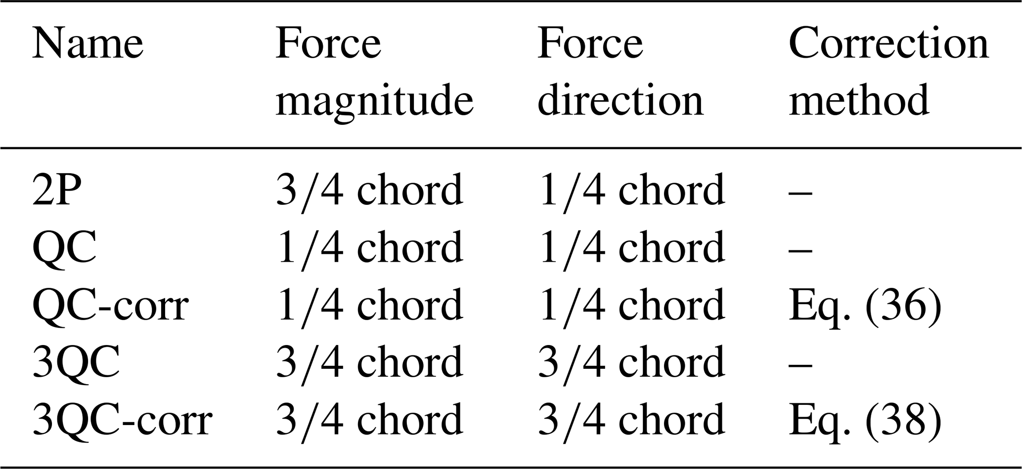
Details of different approaches that are investigated in the present work are summarized in Table 1.

Table 1 Details of different approaches of the generalized lifting-line method that are investigated in the present work. The differences are the chordwise locations where the flow information is used to determine the sectional force magnitude and force direction. The correction methods for different approaches are also listed.

5 Blade geometries for comparison

The blades used for the numerical tests in the present work are based on the IEA-10.0-198 10 MW reference wind turbine (RWT) (Bortolotti et al., 2019). Two different blades are used, which are the baseline straight blade and an upwind dihedral blade. The baseline straight blade is modified by removing the prebend and sweep of the original blade of the RWT so that the main axis of the half-chord line is aligned into a straight line. The upwind dihedral blade is modified from the baseline straight blade so that the half-chord line has out-of-plane shapes. The geometry of the upwind dihedral blade is identical to the W-1 blade in a previous study (Li et al., 2022). The blade has the same radius as the straight blade but is bending upwind from 50 % of radius until the blade tip. The dihedral magnitude is 10 % at the blade tip, and the tip dihedral angle is 20^∘.

In the present work, the test cases are mostly using the baseline straight blade with zero coning, 15^∘ upwind coning and 15^∘ downwind coning. In addition, selected results are presented for an extreme case, represented by the upwind dihedral blade W-1 with added 15^∘ of upwind coning. For the different cases, the main axes of the blades used for the comparison are illustrated in Fig. 4. For the rotor with straight blades and without coning, the radius is 99 m, of which the hub radius is 2.8 m.

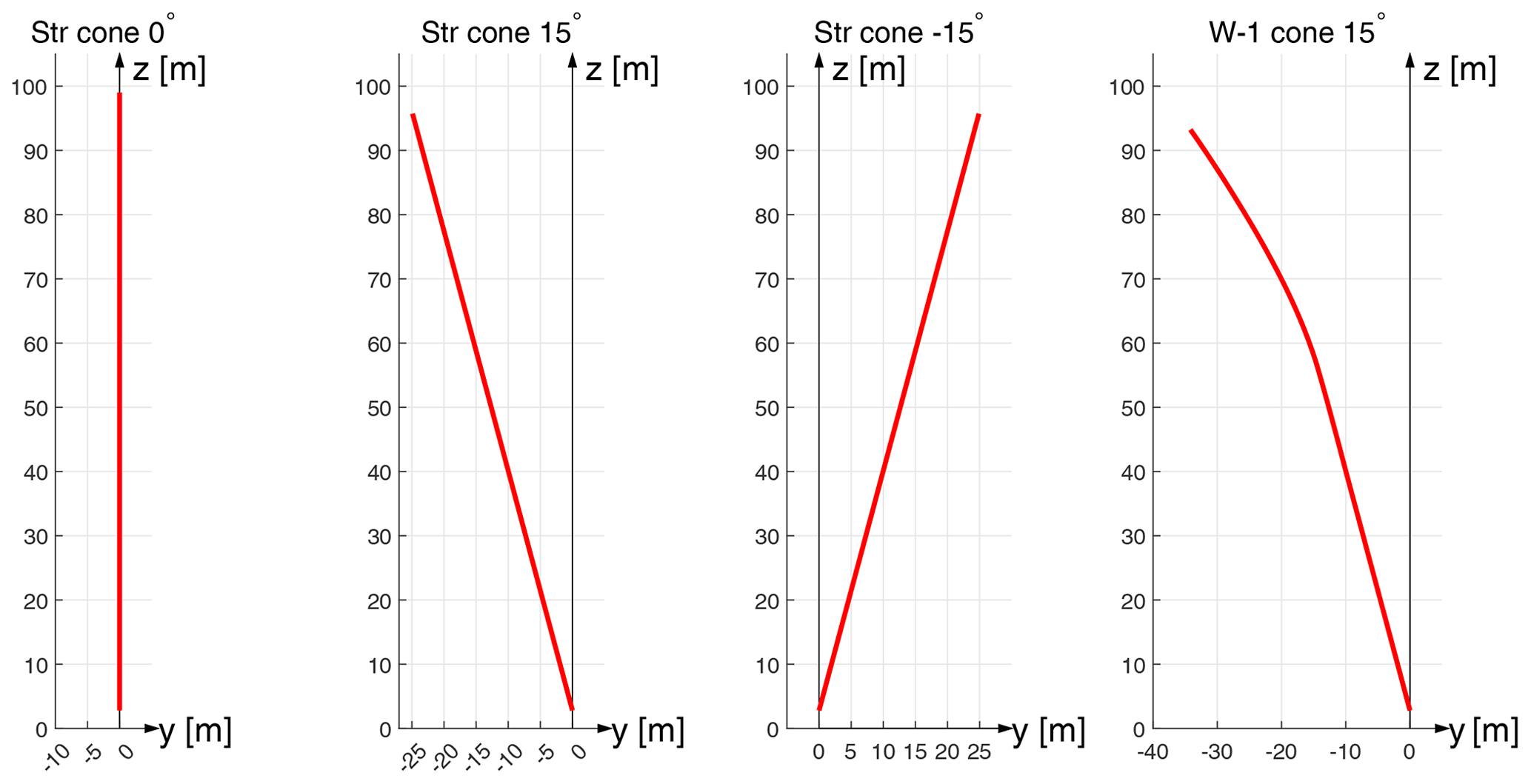
Figure 4 Side view of the main axes of the blades used for different cases of the comparison. The blades from left to right are the baseline straight blade with zero cone angle, 15^∘ upwind coning, 15^∘ downwind coning and the upwind dihedral blade W-1 with added 15^∘ of upwind coning.

6 The aerodynamic models for comparison

In this section, the different aerodynamic models with different numerical fidelities used for comparison are described. The highest-fidelity model used for the comparison is based on blade-geometry-resolving RANS simulations. The generalized lifting-line methods with different fidelities are compared, which are the actuator line (AL) method, the lifting-line (LL) method, the BEVC method and the BEM method. The airfoil data used in all generalized lifting-line methods in the present work are the same, and they were generated with 2-D fully turbulent RANS computations (Bortolotti et al., 2019).

6.1 Fully resolved Navier–Stokes simulations

For the numerical simulations that are used as a reference in the present study, the three-dimensional computational fluid dynamics (CFD) solver EllipSys3D (Michelsen, 1992, 1994; Sørensen, 1995) was used. EllipSys3D solves the incompressible Navier–Stokes equations based on a finite-volume discretization, using structured meshes and a multi-block strategy. A RANS turbulence modeling approach was employed in the present study, relying on the k−ω shear stress transport (SST) model (Menter, 1994). For these fully resolved simulations, body-fitted grids were built around the surface of each of the studied blade geometries, and a wall boundary condition was imposed. Each surface grid was generated using the open-access Parametric Geometry Library (PGL) (Zahle, 2019). The resolution of the surface grids was 256×128 (corresponding to the chordwise direction and the spanwise direction, respectively). Starting from those surface meshes, hyperbolic volume grids were generated with the in-house tool Hypgrid (Sørensen, 1998). A total of 256 cells were generated when marching to the outer limit of the CFD domain, which is located at approximately 11 radii from the surface grid. A boundary layer clustering with an initial cell height of $\mathrm{1}\times {\mathrm{10}}^{-\mathrm{6}}$ m was used, in order to target wall-resolved simulations. Each of the resulting volume meshes had a total of 14.2 million cells. The flow was assumed to be fully turbulent, and an inlet–outlet approach was followed for the boundary conditions of the outer domain. Throughout this document, the body-fitted RANS simulations described here are referred to as fully resolved CFD, or simply CFD. In order to illustrate the mesh topology, Fig. 5 shows a superposition of the grid for the straight blade variants with cone angles of 0 and 15^∘ (upwind).

Figure 5 Detail of the surface mesh for the straight variants used in the fully resolved CFD simulations, showing two of the blades. Two different configurations are included, accounting for a cone angle of 0 and 15^∘. For the zero-cone-angle case, the topology of the volume mesh is shown through arbitrary cross-sectional cuts along the span. The free-stream velocity vector is U₀. For clarity, only every eighth grid line is shown.

6.2 Lifting-line method

The lifting-line module in the aerodynamic solver MIRAS (Ramos-García et al., 2016) is used for comparison. The numerical lifting-line (LL) solver is implemented as a free-wake vortex method in a time-marching fashion. The curved bound vortex influence is modeled by including the difference between the 3-D bound vortex induction and the 2-D bound vortex induction evaluated at the three-quarter-chord point (Li et al., 2020). It should be emphasized that the induced velocity vector due to the curved bound vortex is assumed to be constant along the chord. For the simulations, each time step corresponds to 1.5^∘ of azimuthal rotation. Each simulation is calculated for 20 000 time steps, which corresponds to 83.3 revolutions. The vortex core size is chosen to be 0.1 % of the local chord length. Each blade of the rotor is discretized radially into 50 sections with cosine spacing. Both one-point and two-point approaches of the LL method are implemented.

6.2.1 Two-point approach

The two-point approach in the LL method refers to the explicit calculation of the flow information at both the quarter- and the three-quarter-chord point and is labeled as LL-2P. This approach aligns with the conclusions from the unsteady 2-D thin airfoil theory, as previously described in Sect. 2. The angle of attack at the three-quarter-chord point is used to determine the magnitude of the lift and drag coefficients, whereas the angle of attack at the quarter-chord point is used to determine the direction of lift and drag.

6.2.2 One-point approach

The one-point approaches only use the flow information at a single chordwise location for each section. Two variants of the one-point approach, which are representative of the most common implementations, are used for the comparison. The first one uses only the quarter-chord point as the calculation point (labeled as LL-QC); the second one uses only the three-quarter-chord point (labeled as LL-3QC). The corrections previously described in Sect. 4.1 and 4.2 are implemented for each of the one-point LL methods, respectively. Results corrected accordingly are subsequently labeled as LL-QC-corr and LL-3QC-corr. For LL-3QC-corr, the correction is implemented by including the additional pitch rate drag force as presented in Eq. (38). An overview of different implementations has been summarized in Table 1.

6.3 BEM method

The blade element momentum (BEM) method implemented in the HAWC2 code is the one-point approach that only uses the three-quarter-chord point as the calculation point (Madsen et al., 2020a). The one-point lifting-line correction that is implemented as an additional effective pitch rate drag force described in Sect. 4.2 is already included in the Beddoes–Leishman-type dynamic stall model (Hansen et al., 2004; Pirrung and Gaunaa, 2018) in HAWC2. For the steady-state case, the non-circulatory force has negligible influence, which is shown analytically in Sect. 3 and numerically in Sect. 7.1. As a result, the HAWC2 BEM with the dynamic stall model enabled is labeled as BEM-3QC-corr and is similar to the one-point approach of the LL method with the calculation point placed at the three-quarter-chord line and with the correction (LL-3QC-corr). The HAWC2 BEM that directly uses the quasi-steady aerodynamics is labeled as BEM-3QC and is similar to the one-point approach of the LL method with the calculation point placed at the three-quarter-chord line but without the correction (LL-3QC).

6.4 BEVC method

The blade element vortex cylinder (BEVC) method is the combination of the blade element theory and the vortex cylinder model. It has been shown in a previous work (Li et al., 2022) that the distributed loads of dihedral blades predicted by the BEVC model agree significantly better with higher-fidelity LL and fully resolved CFD than BEM results. In that previous work, it was described that the unsteady airfoil aerodynamic effects are included in the numerical tests, which is actually done by enabling the Beddoes–Leishman-type dynamic stall model when implemented in the HAWC2 code. This means the steady-state results in that previous work already included the one-point lifting-line correction described in Sect. 4. Similar to the HAWC2 BEM module, the BEVC method implemented in HAWC2 also uses the three-quarter-chord point as the calculation point. In the present work, the results with and without the correction are labeled as BEVC-3QC-corr and BEVC-3QC, which are compared to show the importance of the effect.

6.5 Actuator line simulations

Consistent with the fully resolved CFD computations, the actuator line (AL) simulations also used the EllipSys3D flow solver⁵ with the same numerical setup as the fully resolved simulations described in Sect. 6.1. However, instead of employing a body-fitted rotor mesh, the AL (Sørensen and Shen, 2002) distributes the sectional blade forces – computed from 2-D airfoil polars – over a Cartesian box mesh by a three-dimensional Gaussian kernel. This base formulation is enhanced by including the computationally efficient smearing correction described by Meyer Forsting et al. (2019a, b, 2020). Such a correction renders the AL equivalent to a lifting-line, as proven by Meyer Forsting et al. (2019a) and Martínez-Tossas and Meneveau (2019). Without the correction, the AL acts as a LL with a viscous core. In the present work, the smearing correction is partially assuming the rotor to be planar due to the underlying assumptions in the near-wake model (Pirrung et al., 2016).

The numerical domain discretization follows a verified approach (Meyer Forsting et al., 2017; Troldborg et al., 2009) and consists of a box with 50R (R= 99 m) edge lengths that contains a rectangular, uniformly spaced refined mesh with 3.2R side lengths in the cross-flow and 3.9R in the streamwise direction. The rotor is placed in the domain center, with the refined mesh starting 1.6R upstream, as illustrated in Fig. 6. The latter thus surrounds the AL and has a grid spacing of $\mathrm{\Delta }x=R/\mathrm{80}$ to resolve the flow features of interest. The full volume mesh has 75 million cells. The domain boundaries off the main flow direction are of the symmetry type, whereas the inflow and outflow faces obey Dirichlet and Neumann conditions, respectively. To ensure the blade tip remains well inside a single grid cell during each time step, Δt= 0.0117  s. The smearing or kernel length scale is twice the grid size as recommended by Troldborg et al. (2009) to guarantee numerical stability, and the blade is discretized into 100 aerodynamic sections between root and tip. The one-rotation averaged sectional blade forces are converged down to a residual of $\mathrm{1}\times {\mathrm{10}}^{-\mathrm{5}}$.

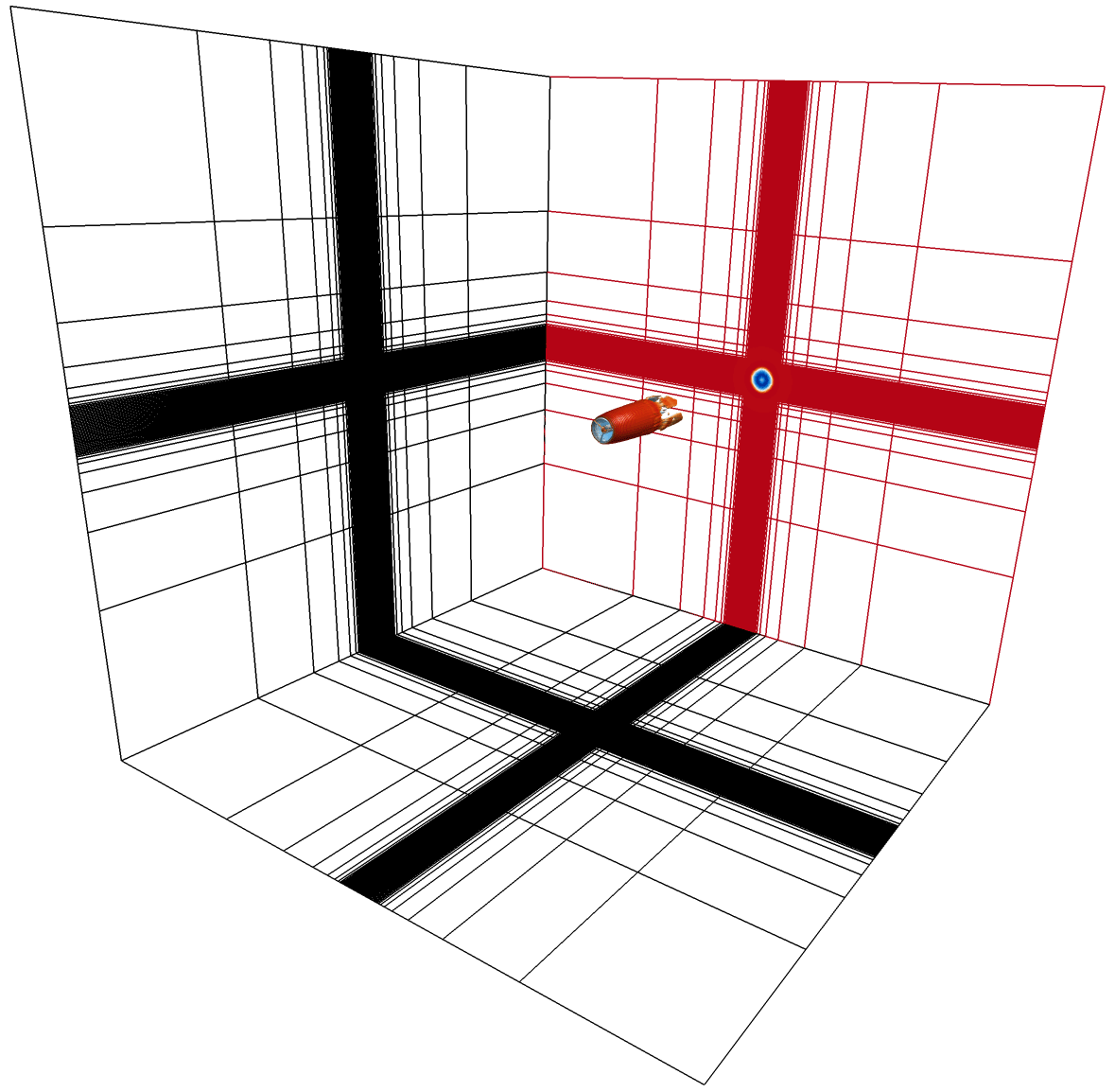
Figure 6 Actuator line numerical box domain with a structured mesh and uniform spacing around the rotor at its center. Only every eighth grid point is shown.

In the AL method, the velocity is only calculated on the actuator line itself. Considering the equivalence between the AL and the LL method for straight blades without coning, the AL method before the one-point correction is similar to the LL method that only uses the quarter-chord locations in the load computations (LL-QC) and is labeled as AL-QC. Similarly, the AL method following the one-point correction should be equivalent to LL-QC-corr, which is labeled as AL-QC-corr.

7 Results

In this section, various numerical tests are performed to investigate the different assumptions outlined in the previous sections and also to evaluate the performance of the one-point lifting-line correction for different aerodynamic models. Firstly, the impact of non-circulatory forces under steady-state conditions is tested using the LL method in Sect. 7.1. Then, the impact of the variation in the relative velocity magnitude along the chord is investigated numerically in Sect. 7.2. Afterwards, the one-point lifting-line correction is tested for different implementations of the LL method in Sect. 7.3, for the BEM method in Sect. 7.4, for the BEVC method in Sect. 7.5 and for the AL method in Sect. 7.6.

For all test cases, the pitch angle is zero, and the rotor is operating under uniform inflow of 8 m s⁻¹ that is perpendicular to the rotor plane. The rotational speed of the rotor is constant at 0.855 rad s⁻¹. For the cases with zero cone angle, the radius is 99 m, and the tip speed ratio is 10.58. At this operational condition, the thrust coefficient of the unconed rotor with baseline straight blades is 0.90, and the rotor power coefficient is 0.46, as predicted using the BEM method.

The initial assessment of the performance of the different numerical methods relies on the study of the sectional aerodynamic load distributions. In order to ensure the quality of the comparison among different blade geometries involved in the present study, it is important to define the loads in a consistent manner. The loads are defined as force per unit radius, which is the same definition used in the previous work (Li et al., 2022). The sectional aerodynamic loads that are calculated from the 2-D airfoil data and projected into the rotor coordinate system should correspond to force per unit curved blade length. The loads with the definition of force per unit radius are obtained by multiplying the curved blade length correction factor $\mathrm{d}s/\mathrm{d}r$ (Madsen et al., 2020a). For the coned straight blade case, the correction factor is equal to the secant of the cone angle. For the dihedral blade with added coning, the correction factor is equal to the secant of the sum of the cone angle and the local dihedral angle (Li et al., 2022).

7.1 The non-circular force at steady state

It is shown analytically in Sect. 3.4 that the total non-circulatory lift of a pure dihedral blade operating under steady-state conditions under uniform inflow perpendicular to the rotor plane is approximately zero. In addition, it is shown in Sect. 2.2.3 that there is a non-circulatory drag force due to the pitch rate caused by the effective pitch rate of the airfoil. It was analyzed that the contribution is also negligible for low- to moderate-reduced-frequency cases. In this section, these two conclusions are tested numerically. This is done by comparing the aerodynamic loads of a pure dihedral blade calculated from the two-point approach of the LL method without non-circulatory forces (LL-2P), with non-circulatory lift (LL-2P-NC1), and with both non-circulatory lift and non-circulatory pitch rate drag (LL-2P-NC2). As has been described previously, the non-circulatory lift is perpendicular to the airfoil, so there will be an effective non-circulatory drag in the flow direction due to the projection of the non-circulatory lift, which is included in both LL-2P-NC1 and LL-2P-NC2. The extreme case of the upwind dihedral blade W-1 with additional 15^∘ of upwind coning is used here to amplify the influence of blade dihedral on the non-circulatory forces. The axial and tangential loads predicted by the two-point LL approach, both with and without the non-circulatory forces, are compared in Fig. 7. In addition, the fully resolved CFD results are included for reference.

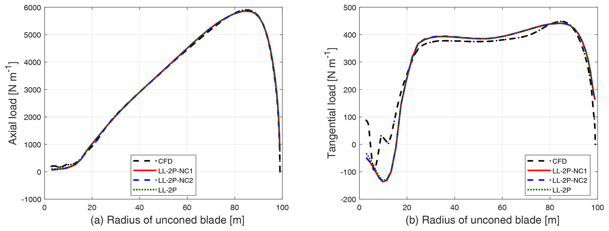
Figure 7 Comparison of axial load (a) and tangential load (b) of the upwind dihedral blade W-1 with additional 15^∘ of upwind coning calculated from the fully resolved CFD and the two-point approach of the LL method without non-circulatory force (LL-2P), with non-circulatory lift (LL-2P-NC1), and with both non-circulatory lift and the non-circulatory pitch rate drag (LL-2P-NC2).

It can be seen from the figure that the loads from the LL method with or without the non-circulatory force are almost identical and are in good agreement with the results from the fully resolved CFD solver. To clearly show the magnitude of the non-circulatory forces, the difference in the loads calculated from LL-2P-NC1 and LL-2P-NC2 with respect to the results from LL-2P is calculated. The difference generally increases when moving from the blade tip to the blade root but is negligible. For the spanwise position between a radius of 40 m (of the unconed blade) to the blade tip, the difference compared to the LL-2P method is within 2 N m⁻¹ for the axial load and is within 5 N m⁻¹ for the tangential load. For the radius of 20 m (of the unconed blade), the difference is within 2 N m⁻¹ for the axial load and is within 12 N m⁻¹ for the tangential load. It should be emphasized that the total non-circulatory force may not be negligible for unsteady cases.

7.2 The variation in relative velocity magnitude

For the generalized lifting-line methods, there are two procedures that involve the magnitude of the relative velocity for the calculation. The first one is the calculation of the quasi-steady bound circulation strength, which is related to the convergence calculation.

$$\begin{array}{}\text{(41)}& \mathrm{\Gamma }={\displaystyle \frac{\mathrm{1}}{\mathrm{2}}}{V}_{\mathrm{rel}}c{C}_{\mathrm{L}}^{\mathrm{QS}}\left({\mathit{\alpha }}_{\mathrm{3}/\mathrm{4}}\right)\end{array}$$

The second one is during the calculation of the lift and drag forces, which is to compute the aerodynamic loads on the blades. This procedure is performed after the convergence calculation and can be considered to be the post-processing of the converged results.

$$\begin{array}{}\text{(42)}& {\displaystyle }{L}^{\mathrm{QS}}={\displaystyle \frac{\mathrm{1}}{\mathrm{2}}}\mathit{\rho }{V}_{\mathrm{rel}}^{\mathrm{2}}c{C}_{\mathrm{L}}^{\mathrm{QS}}\left({\mathit{\alpha }}_{\mathrm{3}/\mathrm{4}}\right)\text{(43)}& {\displaystyle }{D}^{\mathrm{QS}}={\displaystyle \frac{\mathrm{1}}{\mathrm{2}}}\mathit{\rho }{V}_{\mathrm{rel}}^{\mathrm{2}}c{C}_{\mathrm{D}}^{\mathrm{QS}}\left({\mathit{\alpha }}_{\mathrm{3}/\mathrm{4}}\right)\end{array}$$

There is no clear indication from unsteady thin airfoil theory at which chordwise location to extract the relative velocities for any of these two procedures. For the one-point approach, it is natural to use the relative velocity at the calculation point for both procedures. For the two-point approach, it is possible to choose the relative velocity at either the quarter-chord point or at the three-quarter-chord point for both procedures. In total, there are four possible combinations, which are summarized in Table 2.

Table 2 The four different choices of the chordwise location for the magnitude of the relative velocity to use for the calculation of the bound circulation strength and the magnitude of the lift and drag force in the two-point approach of the lifting-line method.

From an intuitive point of view, Case 3 appears as the most correct one because the angle of attack at the three-quarter-chord point is used to determine the lift coefficient, and the flow at the quarter-chord point is used to determine the lift and drag direction. The difference between these four combinations is tested numerically by comparing the loads calculated using different implementations of LL-2P. For this numerical test, the extreme case with the upwind dihedral blade W-1 with 15^∘ of additional upwind coning is used. To clearly show the difference between different implementations, the difference in the loads of the other three methods compared to the intuitively most correct method (Case 3) is plotted in Fig. 8.

Figure 8 Comparison of the difference in axial load (a) and tangential load (b) of the upwind dihedral blade W-1 with 15^∘ of additional upwind coning calculated using the three different methods compared to the intuitive correct method (Case 3) from the two-point LL methods.

It can be seen that the difference in the loads calculated using different methods is extremely small compared to the full loads as shown in Fig. 7 and is thus negligible. For example, at the spanwise location that corresponds to the 70 m radius of the unconed blade, the maximum difference is less than 0.2 % for the axial load and is less than 0.4 % for the tangential load. It is then confirmed numerically that the variation in the relative velocity magnitude along the chord for the calculation of bound circulation and the magnitude of lift and drag forces is a secondary effect. Then, for the two-point approach, the choice of the relative velocity for the two procedures can be arbitrary. The conclusion can also justify that the one-point approach directly uses the relative velocity at the calculation point for both procedures.

7.3 One-point lifting-line corrections

The correction to the generalized one-point lifting-line method described in Sect. 4 is tested numerically using the LL method in this section. The straight blade with 15^∘ of cone upwind or downwind is used here. In addition, the case of the straight blade without coning is also included for reference to show the influence of blade coning.

The two-point approach of the LL method (LL-2P)⁶ is used as the reference method since it coincides with the conclusions from the unsteady 2-D thin airfoil theory. In addition, the fully resolved CFD results are included for reference. Two different simplified one-point approaches of the LL method (LL-QC and LL-3QC), with the calculation point at either the quarter- or three-quarter-chord line, are compared. As is described in Sect. 4.1 and 4.2, the two methods calculate the wrong magnitude of the lift force and apply the lift force in the wrong direction, respectively. The previous two methods with the corrections are LL-QC-corr and LL-3QC-corr. The numerical tests are performed by comparing the aerodynamic loads calculated from these different implementations of the LL methods as well as the fully resolved CFD.

7.3.1 Straight blade without coning

Firstly, the axial and tangential loads of the straight blade without coning calculated from different implementations of the LL method are calculated and are plotted together with the fully resolved CFD results in Fig. 9.

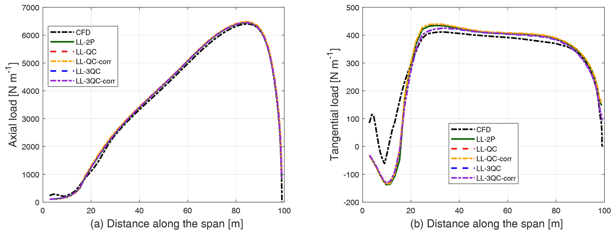
Figure 9 Comparison of axial load (a) and tangential load (b) of the straight blade without coning calculated from different LL methods and the fully resolved CFD.

It can be seen from the figure that the loads from all LL methods give very similar results for both axial and tangential loads. The results in the figures are almost on top of each other. The loads predicted by the LL methods are also in good agreement with the CFD results. At the near-root region (i.e., up to an approximate radius of 20 m), clear differences between the CFD solution and the rest of the methods were observed. These discrepancies are related to the separation in the near-root region predicted by the CFD solver. This effect has a relatively low influence on the integrated loads and is not the subject of the present investigation.

7.3.2 Upwind-coned case

The axial and tangential loads of the straight blade with 15^∘ of upwind coning are calculated from different implementations of the LL method and are plotted together with the fully resolved CFD results in Fig. 10.

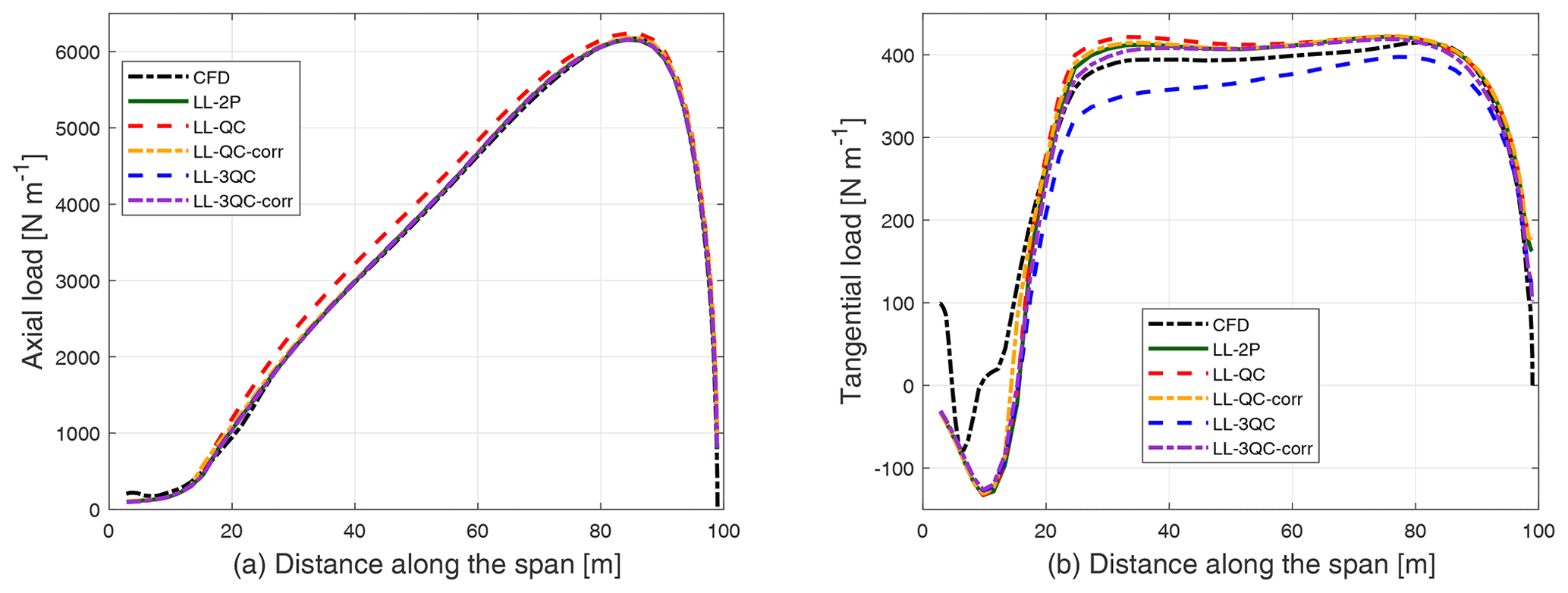
Figure 10 Comparison of axial load (a) and tangential load (b) of the straight blade with 15^∘ of upwind coning calculated from different LL methods and the fully resolved CFD.

It can be seen from the figure that for the axial load, all LL methods except LL-QC give very similar results and are in good agreement with the fully resolved CFD. The axial load is overestimated by LL-QC. For the tangential load, the LL-3QC method predicts a somewhat lower value compared to the other LL methods, while the other methods show only small differences and are in good agreement with the fully resolved CFD. To better illustrate the effect of blade coning predicted by different LL methods, the difference in the loads of the coned straight blade with respect to the baseline straight blade without coning is plotted in Fig. 11.

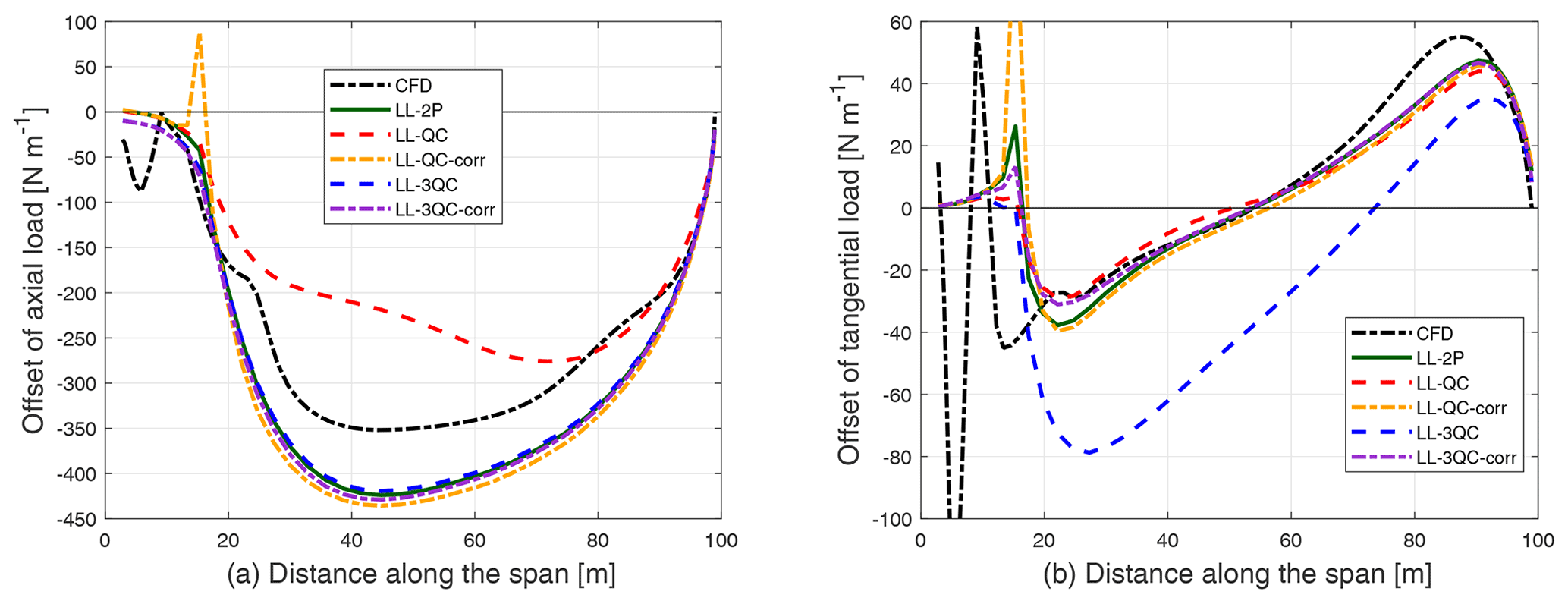
Figure 11 Comparison of the difference in the axial load (a) and tangential load (b) of the straight blade with 15^∘ of upwind coning compared to the straight blade with zero cone angle, calculated from different implementations of the LL method and the fully resolved CFD.

For the LL-QC method, the decrement of the axial load is significantly underestimated compared to the predictions by the LL-2P. This is expected since the magnitude of the lift is not correctly calculated using the LL-QC method. After applying the correction, the axial load from LL-QC-corr agrees significantly better with LL-2P. For the tangential load, the result from LL-QC is in reasonably good agreement with the other methods as despite the magnitude of the lift force having an offset, the lift force is applied in the correct direction.

For the LL-3QC method, the calculated axial load is in good agreement with the result from LL-2P because the magnitude of the lift force is correctly calculated. The tangential load calculated from LL-3QC is underestimated compared to LL-2P. This is because the lift force is not applied to the correct direction in LL-3QC. After applying the correction, the tangential load predicted by LL-3QC-corr is in good agreement with LL-2P.

7.3.3 Downwind-coned case

For the straight blade with 15^∘ of downwind coning, the axial and tangential loads calculated from different LL methods and the fully resolved CFD are plotted in Fig. 12.

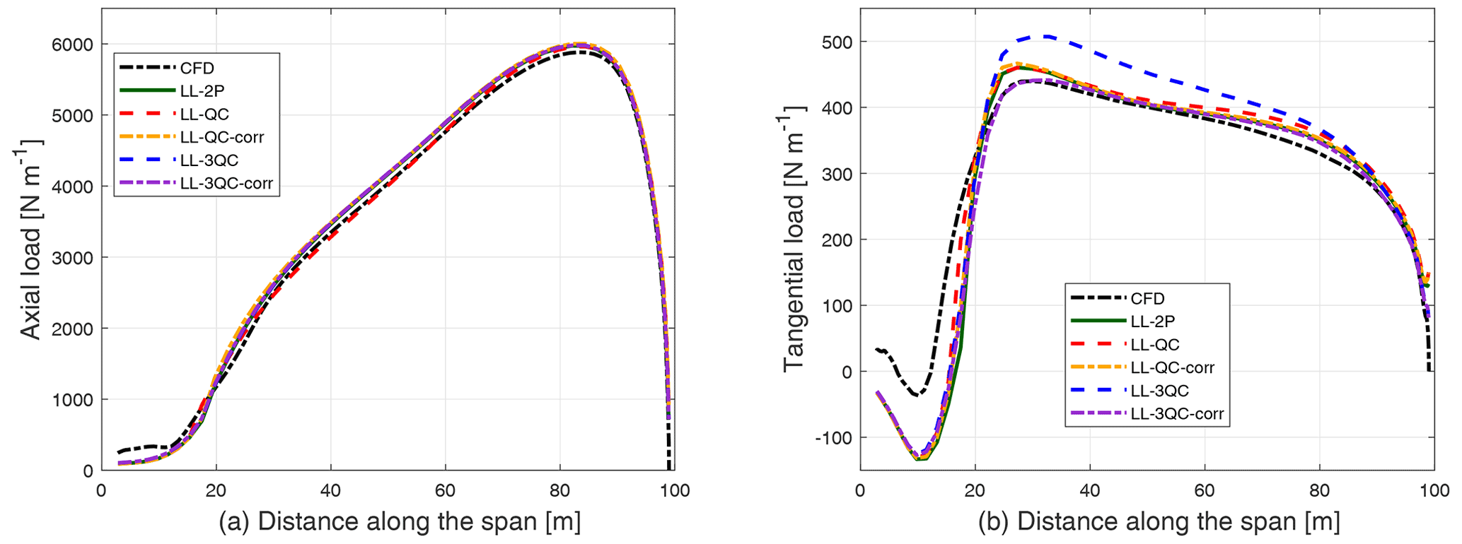
Figure 12 Comparison of axial load (a) and tangential load (b) of the straight blade with 15^∘ of downwind coning calculated from different implementations of the LL method and the fully resolved CFD.

It can be seen from the figure that similar to the case of upwind coning, all LL methods except LL-QC predict almost identical axial loads and are similar to the prediction by the fully resolved CFD. The LL-QC method underestimates the axial load compared to other LL methods. For the tangential load, LL-3QC predicts a significantly higher load compared to the predictions by other LL methods, which only show a small difference between each other and are similar to the fully resolved CFD result. Similar to the upwind-coning case, the difference in the loads of the downwind-coning straight blade with respect to the straight blade without coning calculated from different LL methods and the fully resolved CFD is plotted in Fig. 13 for a detailed comparison.

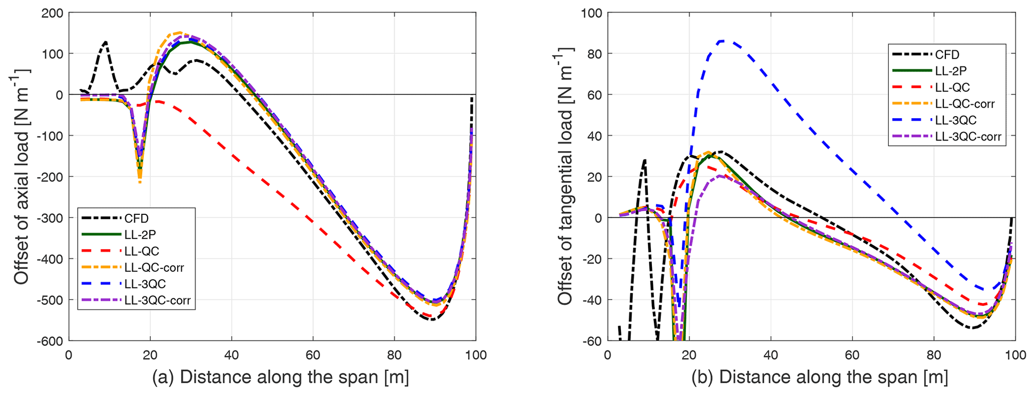
Figure 13 Comparison of the difference in the axial load (a) and tangential load (b) of the straight blade with 15^∘ of downwind coning compared to the straight blade with zero cone angle calculated from different implementations of the LL method and the fully resolved CFD.

For the LL-QC method, the axial load is underestimated and shows a relatively large difference compared to the load calculated using LL-2P. As has been explained for the upwind-coned case, the reason is that the magnitude of the lift is not correctly calculated using LL-QC. On the other hand, the tangential load calculated from LL-QC is slightly overestimated compared to the LL-2P method, but they are still in reasonably good agreement. The reason is, as has been explained for the upwind-coning case, that the lift force is applied in the correct direction despite the magnitude of the calculated lift force having some offsets. After applying the correction, the axial load from LL-QC-corr is now in good agreement with LL-2P. The tangential load predicted by LL-QC-corr is also in improved agreement with LL-2P.

For the LL-3QC method, the axial load is in good agreement with LL-2P since the magnitude of the lift is correctly modeled. However, LL-3QC especially overestimates the tangential load compared to LL-2P. As has been explained for the upwind-coning case, this is because the lift force is not applied to the correct direction and results in an additional effective drag force. After applying the correction, the tangential load calculated from LL-3QC-corr is in significantly improved agreement with LL-2P.

In summary, all of the corrected methods have consistently good performance for either upwind or downwind dihedral cases. The performances of LL-QC-corr and LL-3QC-corr are almost identical to LL-2P, and all of them are categorized as the full model since they align with the conclusions from unsteady 2-D airfoil theory. The important aspect is to use a correction such that the modeling effectively mimics the behaviors according to the thin airfoil theory.

7.4 BEM method

The importance of consistently using the 2-D airfoil data when using the BEM method to calculate the loads of the dihedral blades is tested in this section. Again, the focus is on the special case of a pure dihedral blade without sweep under steady-state operating conditions. The blades for the test are the straight blade with 15^∘ of upwind coning and 15^∘ of downwind coning. In addition, the results of the straight blade without coning are also included as the reference. The axial and tangential loads calculated from BEM with and without the correction (by enabling or disabling the dynamic stall model) are labeled as BEM-3QC-corr and BEM-3QC and are compared in Fig. 14.

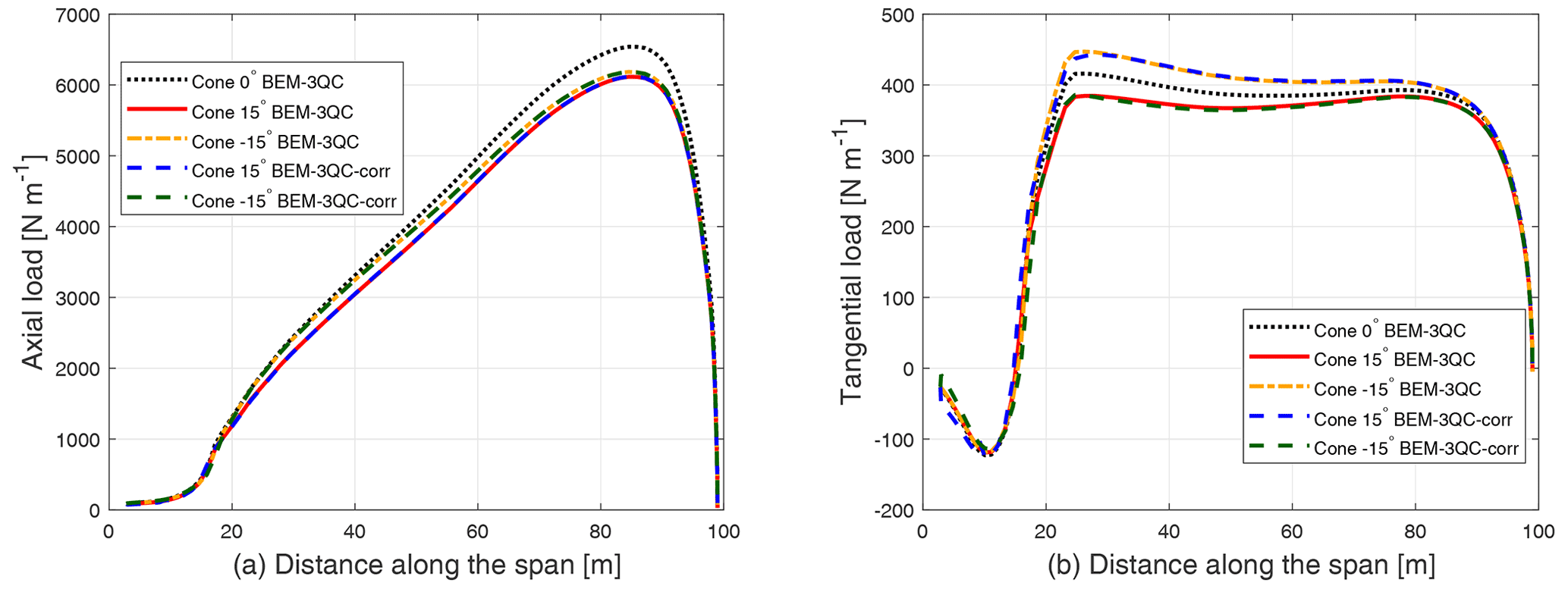
Figure 14 Comparison of axial load (a) and tangential load (b) of the straight blade without coning, with 15^∘ of upwind coning and with 15^∘ of downwind coning (labeled as Cone −15^∘) calculated from the BEM method with and without the one-point lifting-line correction (labeled as BEM-3QC-corr and BEM-3QC). The results of the straight blade without coning are also included for reference.

The axial loads of the upwind-coned blade and the downwind-coned blade have small differences and are lower compared to the blade without coning. For either an upwind- or downwind-coned blade, the axial loads show only a negligible difference with and without the correction. For the tangential load of the coned blades, when including the one-point correction, the results show a relatively large difference compared to using only the quasi-steady aerodynamics. This means that when using the BEM method that only uses three-quarter-chord information and without the correction for a dihedral blade operating under steady-state conditions under uniform inflow, if directly using the quasi-steady aerodynamics, the thrust force is correctly calculated, but there will be a visible error for the predicted aerodynamic power. This conclusion can be generalized to unsteady cases as well. As a result, we recommend the use of the BEM module with the unsteady 2-D airfoil model⁷ enabled, even for steady-state calculations. In the unsteady 2-D airfoil model, the generalized one-point lifting-line correction described in Sect. 4.3 should be included.

A peculiar phenomenon that can be seen in Fig. 14 is that the tangential load of the upwind-coned blade with the correction is very similar to the tangential load of the downwind-coned blade without the correction. Analogously, the tangential load of the upwind-coned blade without the correction is very similar to the tangential load of the downwind-coned blade with the correction. This shows that the BEM method is not able to correctly model the influence of blade dihedral on the 3-D wake and consequently on the aerodynamic loads.

7.5 BEVC method

The importance of the one-point lifting-line correction when using the BEVC method to calculate the loads of the dihedral blades is shown in this section. The blades for the test are also the straight blade with 15^∘ of upwind coning, with 15^∘ of downwind coning, and without coning. The results from the two-point approach of the LL method (LL-2P), which have shown to be in good agreement with the high-fidelity fully resolved CFD for these test cases in Sect. 7.3, are used for the comparison. The BEM results with the one-point correction enabled (BEM-3QC-corr) are also included in the comparison to highlight the performance of the BEVC model. The BEVC method with and without the one-point correction (by enabling or disabling the dynamic stall model) is labeled as BEVC-3QC-corr and BEVC-3QC. For the case of 15^∘ of upwind coning, the difference in the axial and tangential loads compared to the straight blade without coning from different methods is shown in Fig. 15.

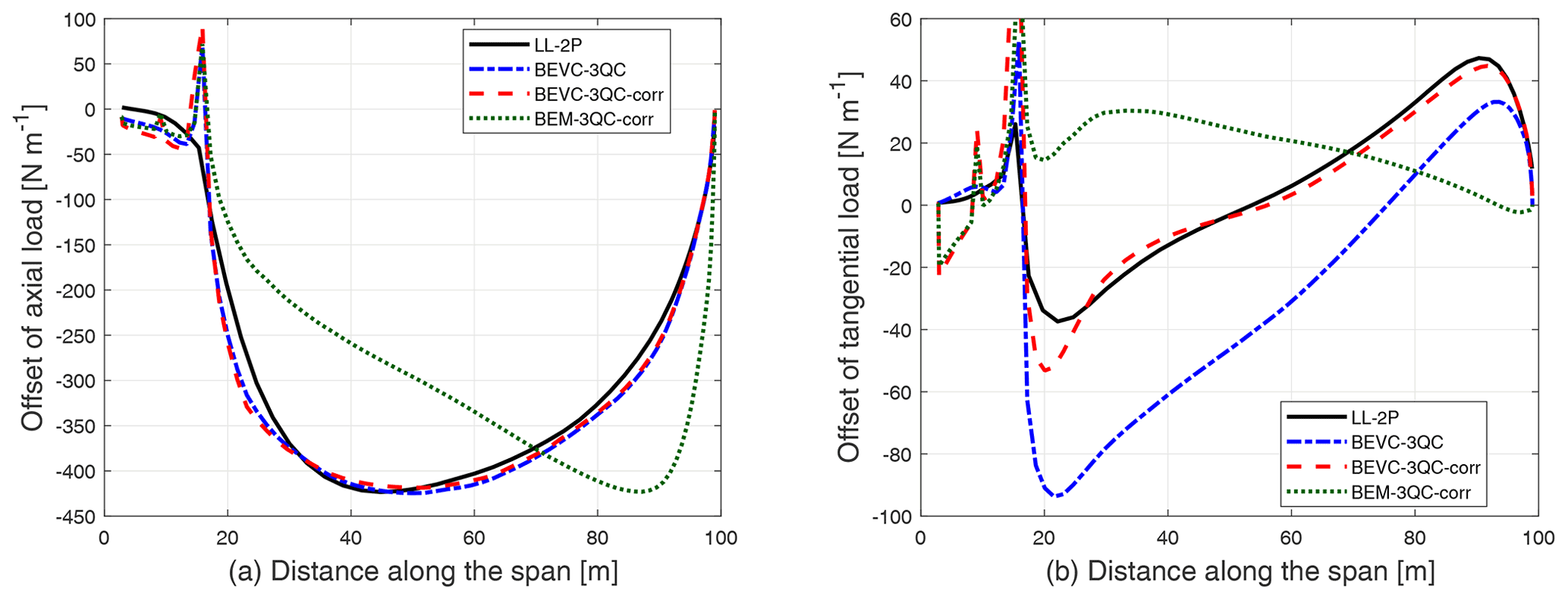
Figure 15 Comparison of the difference in axial load (a) and tangential load (b) of the straight blade with 15^∘ of upwind coning with respect to the straight blade without coning calculated from LL-2P, BEVC with and without the correction (BEVC-3QC-corr, BEVC-3QC), and the BEM method with the correction (BEM-3QC-corr).

For the axial load, the BEVC results with and without the correction are almost identical. This conclusion is the same as for the LL-3QC and the BEM-3QC. The difference in axial loads predicted from BEVC-3QC and BEVC-3QC-corr is in good agreement with the LL-2P. For the tangential load, BEVC-3QC-corr predicts very similar results as the LL-2P. However, if the one-point correction is not included, BEVC-3QC underestimates the tangential loads compared to the predictions by LL-2P. In comparison, BEM-3QC-corr predicts a relatively large difference compared to LL-2P for both axial and tangential loads. This is as expected because the BEM method, even with the one-point correction, is not able to correctly predict the influence of blade out-of-plane geometry on the loads.

For the 15^∘ downwind-coning case, the difference in the axial and tangential loads compared to the straight blade without coning from different methods is shown in Fig. 16.

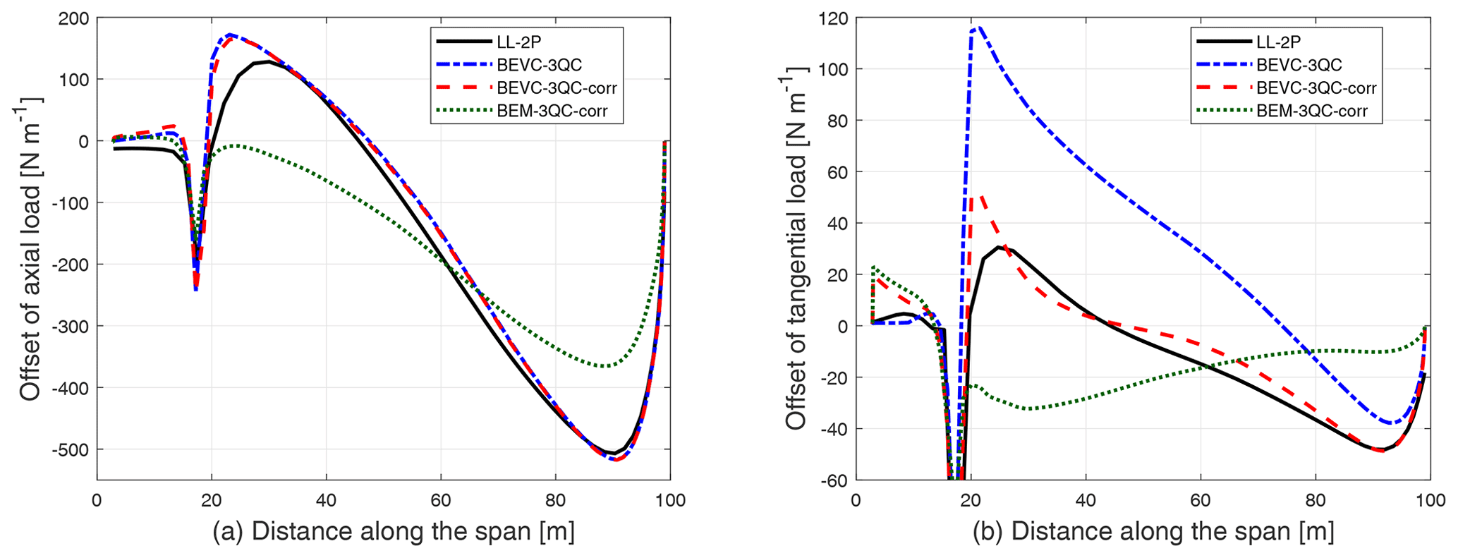
Figure 16 Comparison of the difference in axial load (a) and tangential load (b) of the straight blade with 15^∘ of downwind coning compared to the straight blade without coning calculated from LL-2P, BEVC with and without the correction (BEVC-3QC-corr, BEVC-3QC), and the BEM method with the correction (BEM-3QC-corr).

For the axial load, as for the upwind-coned case, BEVC-3QC and BEVC-3QC-corr have almost identical results and are in good agreement with LL-2P. For the tangential load, BEVC-3QC-corr predicts similar results as the LL-2P. When directly using the quasi-steady airfoil data without the one-point correction, BEVC-3QC overestimates the tangential load. In comparison, BEM-3QC-corr is not able to correctly predict the influence of blade coning on the axial or tangential loads as expected.

7.6 Actuator line method

The actuator line (AL) used in this study is a straight line. This is equivalent to having a straight bound vortex. So, the blades used for the comparison in this section are aligned to a straight quarter-chord line instead of aligned to a straight half-chord line as in the previous sections. The axial load and tangential load of the straight blade with zero cone angle and with 15^∘ of upwind and downwind coning calculated from the AL method without and with the correction (labeled as AL-QC and AL-QC-corr) are compared with results from LL-2P. For the case of a straight blade with 15^∘ of upwind coning, the difference in the axial and tangential loads compared to the straight blade without coning is shown in Fig. 17.

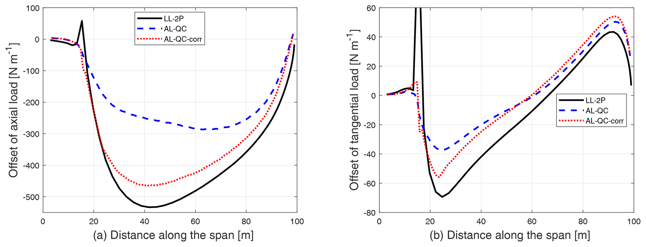
Figure 17 Comparison of the difference in axial load (a) and tangential load (b) of the straight blade with 15^∘ of upwind coning compared to the straight blade without coning calculated from LL-2P, AL without the one-point correction (AL-QC) and AL with the one-point correction (AL-QC-corr).

It can be seen from the figure that the axial load predicted by the AL method without the correction is overestimated compared to LL-2P. This behavior is similar to LL-QC. The tangential load from the AL method is slightly overestimated. After the correction, the axial load from AL-QC-corr is in significantly improved agreement with the result from LL-2P. For the tangential load, the shape of the result from AL-QC-corr is in improved agreement with the result from LL-2P. However, for both axial and tangential loads, the results predicted by the AL-QC-corr method are slightly overestimated compared to LL-2P. This could be related to the smearing correction in the AL method that assumes the calculation point and the trailing point are both in the rotor plane (Pirrung et al., 2016) instead of following the actual blade dihedral geometry.

For the case of 15^∘ of downwind coning, the difference in the axial and tangential loads compared to the straight blade without coning is shown in Fig. 18.

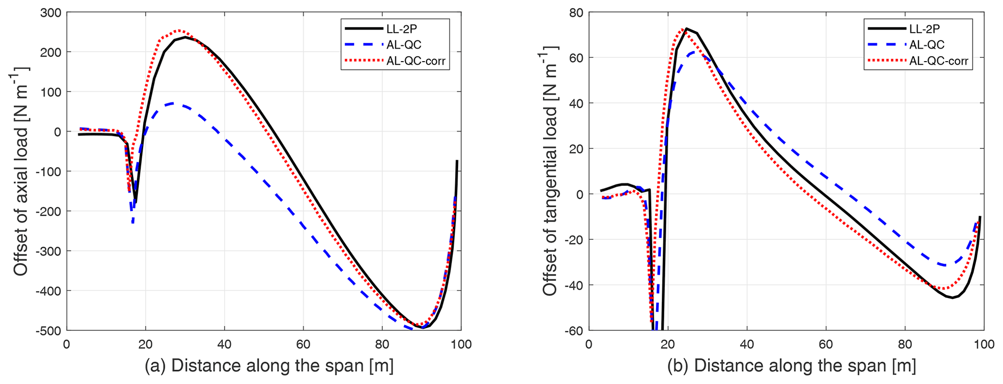
Figure 18 Comparison of the difference in axial load (a) and tangential load (b) of the straight blade with 15^∘ of downwind coning compared to the straight blade without coning calculated from LL-2P, AL without the one-point correction (AL-QC) and AL with the one-point correction (AL-QC-corr).

The AL method without the correction (AL-QC) underestimates the axial load, and the behavior is similar to LL-QC. The tangential load predicted by AL is slightly overestimated compared to LL-2P. After including the one-point correction, the results from AL-QC-corr are in improved agreement with results from LL-2P, for both axial and tangential loads.

7.7 Integrated aerodynamic loads

In addition to the distributed loads that are compared in Sect. 7.3 to 7.6, the importance of the one-point correction for the prediction of the integrated aerodynamic loads (thrust and power) is investigated in this section. The aerodynamic thrust and power in the present work are defined according to the following simplifications, where the forces are assumed to be applied at the main axis, and the contribution of airfoil moment (calculated from C_m) to power is neglected.

$$\begin{array}{}\text{(44)}& {\displaystyle }T=N_{\mathrm{B}}\underset{\mathrm{0}}{\overset{R}{\int }}{F}_{\mathrm{a}}\mathrm{d}r\text{(45)}& {\displaystyle }P:=N_{\mathrm{B}}\underset{\mathrm{0}}{\overset{R}{\int }}r{F}_{\mathrm{t}}\mathrm{d}r,\end{array}$$

where the axial force F_a and the tangential force F_t are with the definition of force per unit radius.

The thrust and power of the rotor with an unconed straight blade as well as the upwind- and downwind-coned straight blades calculated from different aerodynamic models are compared. To better show the influence, the relative difference in thrust and power of the coned rotor with respect to the planar rotor with straight blades is defined as follows:

$$\begin{array}{}\text{(46)}& {\displaystyle }{\mathit{\epsilon }}_T={\displaystyle \frac{T_{\mathrm{cone}}-T_{\mathrm{str}}}{T_{\mathrm{str}}}}\times \mathrm{100}\mathit{\%}\text{(47)}& {\displaystyle }{\mathit{\epsilon }}_P={\displaystyle \frac{P_{\mathrm{cone}}-P_{\mathrm{str}}}{P_{\mathrm{str}}}}\times \mathrm{100}\mathit{\%}.\end{array}$$

The results from different models are summarized in Fig. 19 for the 15^∘ upwind-coned case and in Fig. 20 for the 15^∘ downwind-coned case.

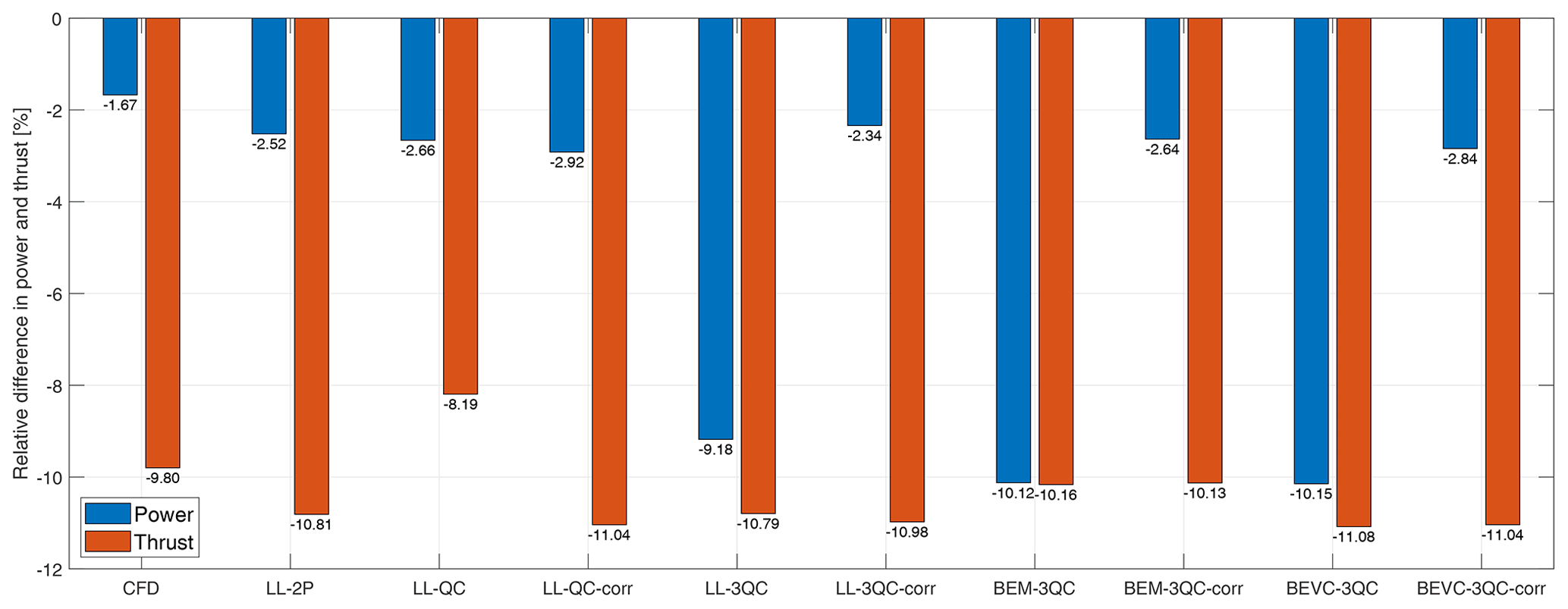
Figure 19 The relative difference in thrust and power of the rotor with straight blade with 15^∘ of upwind coning compared to the zero-cone-angle case.

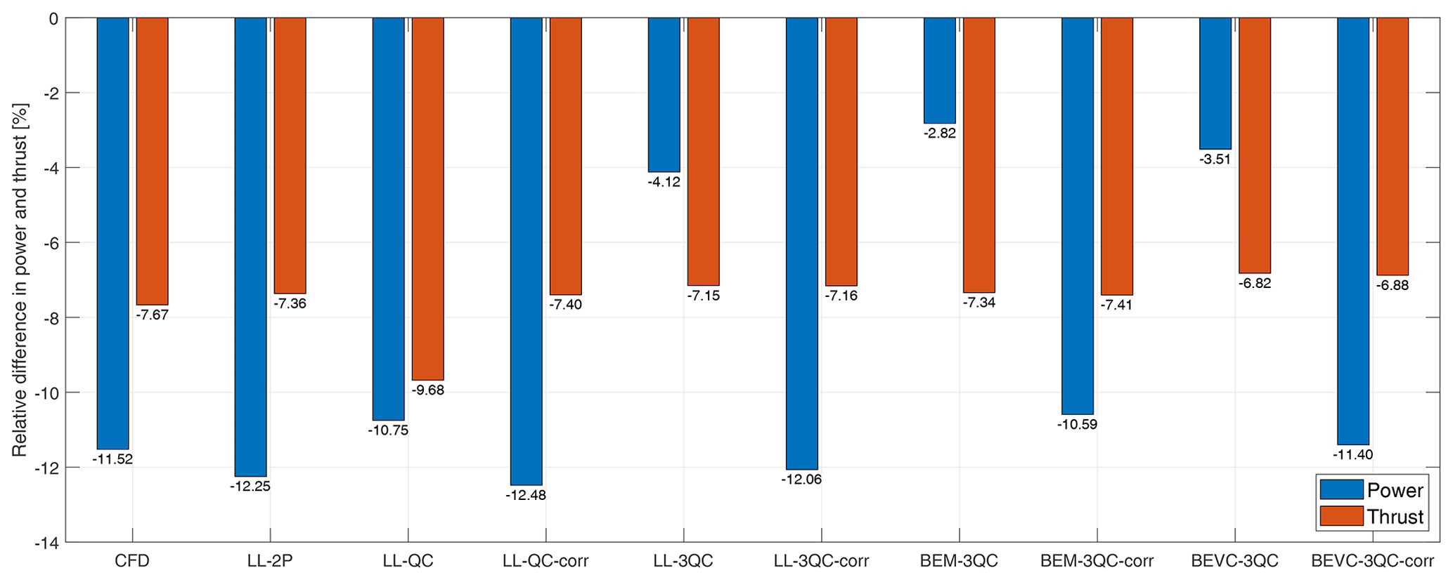
Figure 20 The relative difference in thrust and power of the rotor with straight blade with 15^∘ of downwind coning compared to the zero-cone-angle case.

For all the one-point approaches of the generalized lifting-line method in this comparison, if the one-point correction is applied, the predicted thrust and power of non-planar rotors have reasonably good agreement with the two-point LL method (LL-2P) and the fully resolved CFD. This conclusion also applies to the BEM method. However, if the one-point correction is excluded, and the quasi-steady polars are used directly, the results will have significant errors in either the predicted thrust or power or both, depending on the choice of the calculation point.

It can also be concluded from the results that the BEVC method does not result in significant improvement compared to the BEM method when predicting the integral thrust and power of the coned rotor with straight blades. This is because the influence of the dihedral on the distributed loads is partially canceled out when calculating the power and thrust of the whole rotor. In contrast, the improvement of BEVC over BEM when predicting thrust and power is significant when computing the rotors with curved dihedral blades as shown in the previous work (Li et al., 2022).

For the comparison of the AL method with the LL-2P method, the blades are aligned with the quarter-chord line instead of aligned with the half-chord line. The rotor thrust and power predicted by the AL method with and without the correction and also the LL-2P are summarized in Fig. 21.

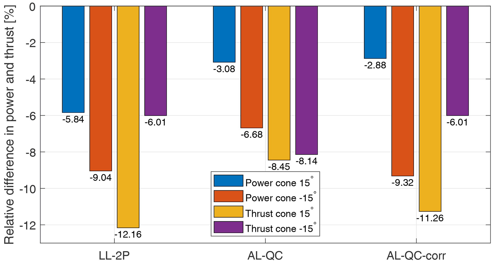
Figure 21 The relative difference in thrust and power of the rotor with 15^∘ upwind- and downwind-coned straight blade aligned to the quarter-chord line compared to the rotor with the same straight blade without coning predicted by the LL-2P method, the AL method without the correction (AL-QC) and the AL method with the correction (AL-QC-corr).

For the AL method without the one-point correction (AL-QC), the thrust is overestimated for the upwind-coned case and is underestimated for the downwind-coned case. The thrust predicted by the AL method with the correction (AL-QC-corr) is in better agreement with LL-2P for both upwind- and downwind-coned cases. The power predicted by AL-QC is overestimated compared to LL-2P for both upwind- and downwind-coned cases. After the correction, the power of the downwind-coned case is in improved agreement with LL-2P but is not improved for the upwind-coned case. As is described in Sect. 7.6, this could be related to the current smearing correction method in the AL model, and future work is needed.

It is worth mentioning that the power and thrust of the cases with coned straight blades that are aligned to a straight half-chord line in Figs. 19 and 20 have relatively large differences from the cases with the straight blades with the same cone angle but aligned to a straight quarter-chord line as in Fig. 21. The difference is approximately 1.3 % in thrust and approximately 3.3 % in power, for both upwind and downwind cases. For the zero-cone-angle cases, the results of both blades are almost identical. For the coned cases, the blades with the two different methods of blade alignment are operating at different angles of attack. For example, at the spanwise location of 40 m, the angle of attack of the quarter-chord-aligned blade is 0.2^∘ smaller compared to the half-chord-aligned blade for the 15^∘ upwind-coned case and is 0.2^∘ larger for the 15^∘ downwind-coned case.

The numerical tests in this section are performed on the straight blades with 15^∘ of upwind and downwind coning, which have significantly non-planar shapes. For the same straight blade under the same operating conditions but with a smaller cone angle, the offset of power and thrust predicted using different generalized one-point lifting-line methods can be approximated from the results in Figs. 19 and 20. Because for the special condition that the blade has only out-of-plane dihedral and no sweep, the pitch rate of the effective airfoil pitching motion $\dot{\mathit{\theta }}$ is proportional to the cone angle κ as shown in Eq. (26), with the small-angle approximation. And for the blade sections that are operating at the linear region, the offset of lift and drag and consequently of the axial and tangential loads is then also approximately linearly proportional to the cone angle. For example, for the same straight blade that is aligned to the half-chord line and has 5^∘ of upwind coning, the relative error in power predicted by LL-3QC is inferred to be approximately 2 %.

8 Conclusions and future work

The present work describes a method where the use of key results from the 2-D unsteady thin airfoil theory results in improved performance of generalized lifting-line methods for non-planar rotors. The conclusions from the unsteady 2-D thin airfoil theory, which are that the magnitude of the quasi-steady lift should be determined by the flow at the three-quarter-chord point, and the direction of the quasi-steady lift should be determined by the flow at the quarter-chord point, are highlighted. The impact of the simplification that using only one calculation point and directly using quasi-steady 2-D airfoil data as usually implemented in generalized lifting-line models is investigated. The generalized correction for such a one-point approach is given. The numerical results from the lifting-line (LL) method, the actuator line (AL) method, the blade element momentum (BEM) method and the blade element vortex cylinder (BEVC) method are compared with and without the correction. The results from fully resolved RANS are also included for reference. The results show a large offset on the prediction of the aerodynamic performance of non-planar rotors when only using the quasi-steady aerodynamics and excluding the one-point corrections. The one-point approaches with the correction are in significantly better agreement with high-fidelity CFD results than without the corrections, for both the distributed loads and the rotor thrust and power. It is noted that the effect of the corrections is modeled correctly by a consistently implemented 2-D airfoil aerodynamic model, such as the Beddoes–Leishman-type model in HAWC2. For this reason, it is suggested to keep such models active also for the simulation of steady-state HAWT rotors with dihedral blades.

There are several future works that are of great interest. Firstly, the comparison of the prediction of the unsteady loads using the two-point approach and the one-point approach of the lifting-line method is interesting. Secondly, the impact of correctly determining the magnitude and direction of the lift force for the curved blade with both sweep and dihedral should be investigated. Thirdly, future work on the actuator line model is necessary for the model to correctly predict the loads of blades with complex shapes. An updated smearing correction for actuator lines with curved shapes is an example.

Appendix A: Nomenclature

a	Non-dimensioned pitching axis location
a	Centrifugal acceleration vector
b	Half-chord length
c	Chord length
C(k)	Theodorsen lift deficiency function
CL	Lift coefficient
CD	Drag coefficient
Cm	Moment coefficient
D	Drag force
Fa	Axial force, with the definition of force per
	unit length radius
Ft	Tangential force, with the definition of force per
	unit length radius
Ftot	2-D total force
k	Reduced frequency
L	Lift force
N	2-D normal force
NB	Number of blades
p	Position vector of the calculation point
P	Aerodynamic power of the rotor
R	Radius of the rotor
T	2-D tangential force, aerodynamic thrust of the rotor
T	Transformation matrix
U0	Free-wind speed
V	Free-stream speed
V3−D	Total 3-D velocity vector
Vrel	Relative velocity
w	Upwash
$\dot{x}$	Streamwise motion of the airfoil
$\ddot{x}$	Streamwise acceleration of the airfoil
$\dot{y}$	Heave motion of the airfoil
$\ddot{y}$	Heave acceleration of the airfoil
Greek letters
α	Angle of attack
$\stackrel{\mathrm{̃}}{\mathit{\alpha }}$	Approximated angle of attack
Δαr	The difference between the reference angle and
	the geometric flow angle
Γ	Bound vorticity strength
ε	Relative difference
ϵ	Normal coordinate of the 2-D airfoil
θ	2-D geometric flow angle
$\dot{\mathit{\theta }}$	Airfoil pitch rate
$\ddot{\mathit{\theta }}$	Airfoil pitching acceleration
κ	Dihedral angle
ξ	Chordwise coordinate of the 2-D airfoil
ρ	Density of air
ϕ	Sectional flow angle
Ω	Rotor speed
Ω	Rotational velocity vector
Subscripts
$\mathrm{1}/\mathrm{4}$	At the quarter-chord point
$\mathrm{3}/\mathrm{4}$	At the three-quarter-chord point
a	In the axial direction
t	In the tangential direction
r	Relative value
i	Induced value
str	Straight blade
cone	Coned blade
heav	Due to heaving motion
stream	Due to streamwise acceleration
acc	Due to acceleration
pitchrate	Due to pitch rate
Superscripts
B	In blade coordinate system
C	Circulatory part
L	In local flow coordinate system
NC	Non-circulatory part
QS	Quasi-steady
S	In sectional coordinate system

Appendix B: An extreme example: VAWT operating in zero onset flow

In this section, in order to shed light on the aspect that is described in Sect. 2.2.4, the extreme case where ideal 2-D thin airfoil sections are mounted on a spinning vertical-axis wind turbine (VAWT) operating with zero onset velocity is investigated. The airfoils are set at an angle such that a constant outward lift is generated due to the relative wind speed from the rotation of the VAWT. Please note that $(V-\dot{x})=V_{\mathrm{rel}}=\mathrm{\Omega }R$, where Ω and R are the angular speed and radius of the VAWT, respectively. In this case, the flow situation as observed from the airfoil section does not change over time, causing the induced drag term to vanish. In addition, there is no streamwise acceleration $\ddot{x}$ or pitching acceleration $\ddot{\mathit{\theta }}$ of the airfoil. The steady situation does have a constant and nonzero pitch rate and heave acceleration $\dot{\mathit{\theta }}=-\mathrm{\Omega }$ and $\ddot{y}=-{\mathrm{\Omega }}^{\mathrm{2}}R$. When evaluating the terms in the non-circulatory lift in Eq. (3), it is seen that the pitch rate term exactly cancels out the heave acceleration term, such that the total lift contains only the circulatory part. Due to the steady nature of the setup, the circulatory lift is equal to the quasi-steady lift, which in turn is freely adjustable by setting the constant angle of the airfoil on the VAWT. Turning now to the drag, it can be seen that all terms in the quarter-chord reference drag in Eq. (14) vanish, resulting in a thin airfoil quarter-chord drag of exactly zero. This is in agreement with the steady-state 2-D thin airfoil drag of zero following d'Alembert's paradox. If evaluating instead the three-quarter-chord reference drag value obtained from Eq. (16),

$$\begin{array}{}\text{(B1)}& D_{\mathrm{3}/\mathrm{4},\mathrm{VAWT}}=L{\displaystyle \frac{b\dot{\mathit{\theta }}}{(V-\dot{x})}}=-L{\displaystyle \frac{c}{\mathrm{2}R}}.\end{array}$$

In non-dimensional coefficients this corresponds to a 2-D drag coefficient of $C_{D,\mathrm{3}/\mathrm{4},\mathrm{VAWT}}=-C_{\mathrm{L}}c/\left(\mathrm{2}R\right)$. As mentioned above, the mounting angle of the airfoil on the spinning VAWT can be freely adjusted to obtain lift coefficients of either positive or negative signs as desired. This also means that in this case the correct value of the three-quarter-chord reference drag may even be a constant negative value. As stated in Sect. 2.2.4, this situation describes the same physics as well as the same force magnitude and direction no matter what reference is used to define the drag force. It is the change in reference direction that makes the three-quarter-chord reference drag value seem counterintuitive. For this reason, it is suggested to use the quarter-chord reference direction definition of the drag coefficient in aeroelastic codes. Figure B1 shows schematically the two implementations described previously.

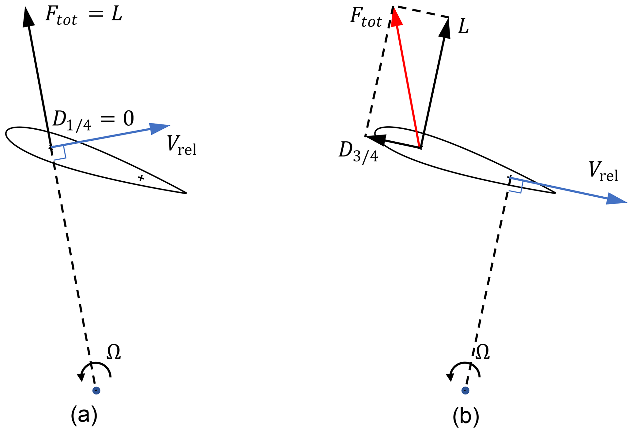
Figure B1 Illustration of two correct methods of defining the direction of the lift and drag forces for a VAWT. (a) Correctly using $D_{\mathrm{1}/\mathrm{4}}$ and relative direction at the quarter-chord point. (b) Correctly using $D_{\mathrm{3}/\mathrm{4}}(<\mathrm{0})$ and relative direction at the three-quarter-chord point. The total force vector in the two cases is identical.

As the last point in this section it should be mentioned that applying the erroneous definition of the direction of the forces in the VAWT case will lead to an effective drag error in the magnitude. For example, for the case of using the three-quarter-chord reference direction but using $D_{\mathrm{1}/\mathrm{4}}$ instead of $D_{\mathrm{3}/\mathrm{4}}$, there will be an effective drag error as given by Eq. (B1). It can be illustrated in Fig. B1b that the erroneous total force will be L instead of F_tot. For this reason an erroneously implemented model may show that it is possible for a VAWT to produce positive aerodynamic power even without an onset flow, as also observed by Pirrung and Gaunaa (2018).