the Creative Commons Attribution 4.0 License.
the Creative Commons Attribution 4.0 License.
 | 07 Jul 2022
Including realistic upper atmospheres in a wind-farm gravity-wave model
Luca Lanzilao
Sebastiaan Jamaer
Nicole van Lipzig
Johan Meyers
Recent research suggests that atmospheric gravity waves can affect offshore wind-farm performance. A fast wind-farm boundary layer model has been proposed to simulate the effects of these gravity waves on wind-farm operation by Allaerts and Meyers (2019). The current work extends the applicability of that model to free atmospheres in which wind and stability vary with altitude. We validate the model using reference cases from literature on mountain waves. Analysis of a reference flow shows that internal gravity-wave resonance caused by the atmospheric non-uniformity can prohibit perturbations in the atmospheric boundary layer (ABL) at the wavelengths where it occurs. To determine the overall impact of the vertical variations in the atmospheric conditions on wind-farm operation, we consider 1 year of operation of the Belgian–Dutch wind-farm cluster with the extended model. We find that this impact on individual flow cases is often of the same order of magnitude as the total flow perturbation. In 16.6 % of the analyzed flows, the relative difference in upstream velocity reduction between uniform and non-uniform free atmospheres is more than 30 %. However, this impact is small when averaged over all cases. This suggests that variations in the atmospheric conditions should be taken into account when simulating wind-farm operation in specific atmospheric conditions.
- Article
(3203 KB) - Full-text XML
- BibTeX
- EndNote


In recent years, it has been well documented that wind farms form a blockage to the flow in and around them (Bleeg et al., 2018), thereby displacing the atmospheric boundary layer (ABL). Such displacements can propagate through the overlying inversion layer and free atmosphere as waves in stably stratified atmospheres, conditions which frequently occur at sea. As offshore wind farms in Europe increase in size and installed capacity (WindEurope, 2018), improving the understanding and simulation of gravity-wave–wind-farm interaction becomes crucial to optimizing turbine control and wind-farm layout (see, e.g., Lanzilao and Meyers, 2021b).
Previous work on the interaction between gravity waves and wind farms has assumed the free atmosphere to be uniformly stratified, with a constant background wind (Smith, 2010; Allaerts and Meyers, 2017, 2019). However, for waves with a horizontal scale of a few kilometers, such as those triggered by wind-farm blockage, vertical variations in the atmospheric conditions can drastically influence the pressure feedback they induce (Teixeira et al., 2013). Therefore, the goal of this work is to determine how variations in the free atmosphere's properties with altitude affect the interaction between gravity waves and the flow in the ABL and overall wind-farm performance.
Allaerts and Meyers (2019) proposed a model focused on the interaction between wind turbines and gravity waves. Based on earlier work by Smith (2010), the model explicitly simulates the flow in the ABL as two height-averaged horizontal layers and incorporates the free atmosphere as a boundary condition. This boundary condition links variations in ABL height to the pressure gradients induced by the corresponding gravity waves. In Fourier space, the relation between these height and pressure perturbations is defined by the stratification coefficient . As the model is based on a three-layer representation of the atmosphere, it is called the three-layer model (TLM).
Currently, the TLM can only describe uniformly stratified free atmospheres, which places a strong restriction on the atmospheric conditions that can be represented. This work adapts the TLM for flow profiles that vary with altitude and studies how these variations change the interaction between the ABL flow and gravity waves. A common approach in gravity-wave theory is to use a piecewise representation of the upper atmosphere, where the profiles of the stratification and the wind speed are split up in a discrete number of layers (Tolstoy, 1973; Gossard and Hooke, 1975; Baines, 1998; Smith et al., 2002; Teixeira et al., 2013; Yu and Teixeira, 2015). We generalize this approach by allowing for an arbitrarily large number of layers so that any atmospheric profile can be accurately analyzed.
It is well known that variations in the atmospheric state can cause wave reflection, which might lead to internal gravity-wave resonance (Gill, 1982). Using the extended TLM, we examine how this resonance affects the pressure feedback on the ABL. Extensive research has been performed on internal gravity-wave resonance, with most of it focusing on flow around topographies, mountain waves, and the effect on the free atmosphere (Teixeira, 2014). As a result, the vertical displacement is simply given by the shape of the topography, not by a change in ABL height. In wind farms, this is different: the displacement is given by a change in ABL depth due to wind-farm blockage, in which the induced gravity waves can play an active role. We therefore set up a qualitative analysis of the feedback loop between ABL flow perturbations and the associated resonant gravity-wave feedback. Finally, in order to estimate the overall effect of vertical variations in the atmospheric conditions, 1 year of operation of the Belgian–Dutch wind-farm cluster is simulated.
The remainder of this paper is organized as follows. Section 2 reviews how gravity waves and the ABL flow interact and how the TLM models ABL flow. In Sect. 3, the analytical expressions for the stratification coefficients for non-uniform atmospheres are derived. To evaluate these, a method for solving the wave equation has to be developed, which is done in Sect. 3.2. Section 4 uses the developed method to analyze the effect of variations in the wind and stability in the free atmosphere on wind-farm operation. Finally, the paper concludes with a summary and suggestions for further research in Sect. 5.
Wind farms form a blockage to the ABL flowing through and around them, thereby pushing the inversion layer, and the free atmosphere above, upwards. These displacements can trigger gravity waves, which may influence the ABL flow by inducing pressure gradients. The first part of this section discusses these induced pressures, while the second part gives an overview of how the TLM models ABL flow and how it incorporates gravity-wave effects.
2.1 Pressure feedback induced by gravity waves
The vertical displacement ηt of the capping inversion topping the ABL leads to two types of atmospheric gravity waves. The first type, called inversion gravity waves, propagate horizontally along the inversion layer, similar to surface water waves. Due to the strong stratification in the inversion layer, any vertical displacement ηt of the inversion layer will be counteracted by the buoyancy-generated changes in pressure (Gill, 1982; Smith, 2010):
where is the unperturbed density, and is the reduced gravity, determined by the potential temperature θ and the inversion strength Δθ.
The second type of waves propagates vertically through the free atmosphere above the capping inversion if it is stably stratified, as is usually the case. The free atmosphere perceives ηt similarly to large-scale topographies, and internal gravity waves are generated (Smith, 2010). In return, the internal gravity waves also induce pressure gradients on the ABL. This pressure feedback is easily expressed by using double Fourier transforms in the horizontal directions (i.e., ) of the displacement and the pressure. For each wavenumber (k,l), the perturbation in the free atmosphere is a plane wave, with the vertical velocity given by Nappo (2012):
where is the intrinsic frequency of the gravity waves, with and the x and y components of the background velocity, and where m is the vertical wavenumber of the internal gravity waves. For each separate wavenumber (k,l), the pressure perturbation of the plane wave is proportional to the ABL displacement , with the relation determined by the stratification coefficients (Smith, 2010):
For uniform free atmospheres, these coefficients are given by Smith (2010):
where is the Brunt–Väisälä frequency, which is constant with height in the uniform case. Further, m can be found using the dispersion relation (Gill, 1982):
If , then m2 is positive, and the waves propagate vertically. If , then m2 is negative, and the waves become evanescent. To find Φ, the sign of m has to be known. For propagating waves (m2>0), the sign of m is determined by the radiation condition, which states that the energy flux of a wave, which is directed along , should be upwards, away from the perturbation (Baines, 1998). It then follows that . For evanescent waves (m2<0), the positive root has to be chosen for the perturbation to die out with altitude (Smith, 1980).
2.2 Three-layer model
The TLM is based on earlier work by Smith (2010), who first analyzed the impact of gravity waves on wind-farm operation. It represents the ABL as being neutrally stable and capped by an inversion layer, with the flow above being stably stratified. Although stably stratified atmospheres have often been modeled this way (Klemp and Lilly, 1975; Durran, 1990; Vosper, 2004; Smith, 2007; Sachsperger et al., 2015), Smith (2010) was the first to apply such a model to wind-farm operation. His model assumes that the flow in the ABL does not vary with height so that the perturbed variables can be replaced by their height averages. As a result, horizontal flow divergence and convergence will lead to changes in the ABL height. Another assumption is that the ABL flow is assumed to be hydrostatic. The inversion layer is modeled as a zeroth-order jump in potential temperature Δθ at the top of the ABL, and the free atmosphere above is assumed to be uniformly stratified.
The TLM improves on the model by Smith in several ways, the most important of which is to divide the ABL in two separate layers. The resulting lower and an upper layer are denoted by subscripts 1 and 2, respectively. The two layers are separated by a pliant surface, similar to the interface between the ABL and the free atmosphere. The wind-farm forcing terms are added in the momentum equations for the lower layer while only affecting the upper layer through interaction through the pliant surface. For this reason, the lower layer is also called the wind-farm layer. The resulting approximation of the ABL is visualized in Fig. 1. The flow in the two layers is governed by the following two-dimensional depth-averaged linearized momentum and continuum equations (Allaerts and Meyers, 2019):
The atmospheric base state is governed by the mean depth-averaged wind speeds and (with ) and the layer heights H1 and H2 of the wind farm and upper layer, respectively, and , , η1, and η2 represent the perturbations to this reference state. The total inversion layer displacement ηt is given by the sum of η1 and η2. Following Allaerts and Meyers (2019), H1 is taken to be twice the hub height of the turbines throughout this work. Further, is the perturbation of the velocity difference between the wind farm and the upper layer, linked to the perturbation of the friction at the interface by the matrix Dij. Similarly, the matrix Cij relates the perturbation of the friction at the ground to the velocity perturbations in the lower layer. Finally, fc is the Coriolis parameter, and Fi is the wind-turbine-forcing term.
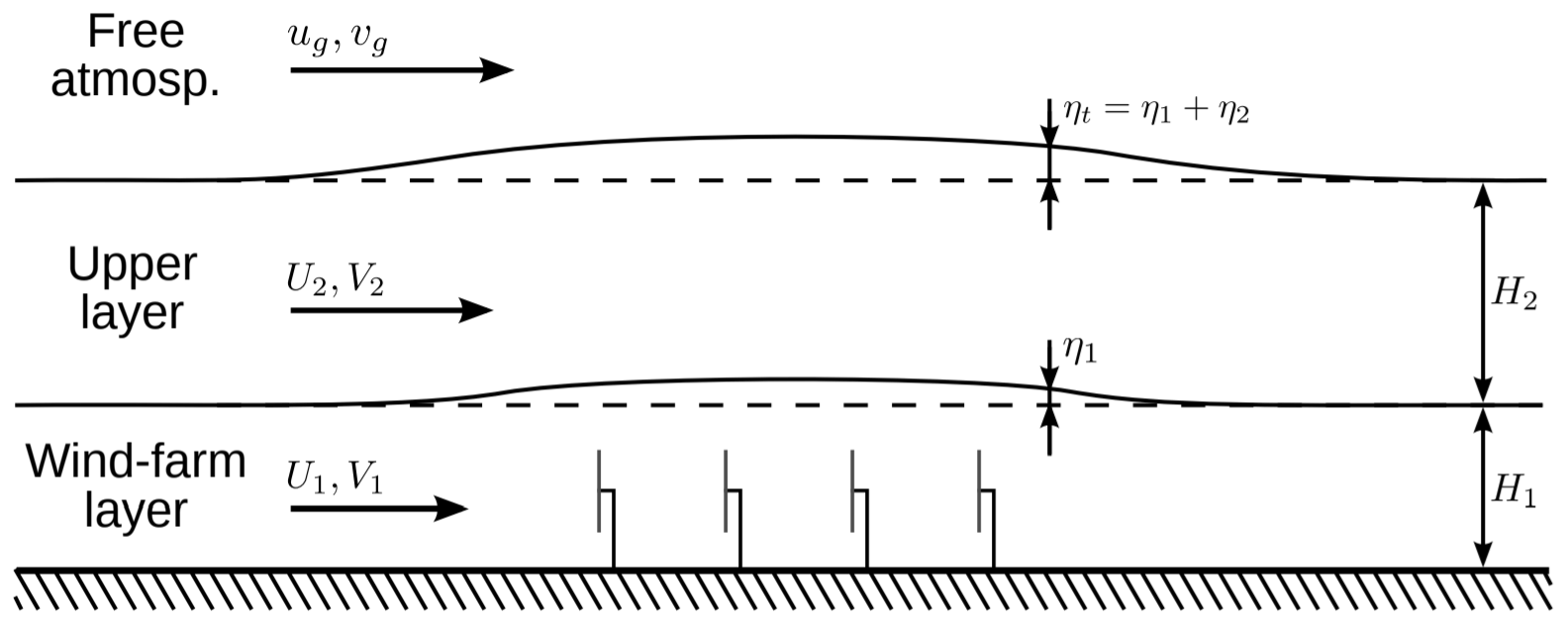
Figure 1Schematic representation of the three-layer model. Figure from Allaerts and Meyers (2019), reproduced with permission.
In Eqs. (6)–(9), the pressure has been substituted using the equations discussed in Sect. 2.1. As the ABL is assumed to be hydrostatic, the pressure perturbation is equal to the pressure induced by the gravity waves generated by the changes in ABL height :
where * is the convolution operator. In this way, the TLM incorporates the gravity-wave effects through a pressure boundary condition, which is determined by the stratification coefficients Φ. These coefficients do not depend on the values of ηt or p′ and can thus be calculated separately from the set of Eqs. (6) to (9). To avoid the computationally expensive convolution, the TLM is solved using a spectral method with a Fourier–Galerkin discretization (Allaerts and Meyers, 2019). Finally, we note that the hydrostatic assumption in the boundary layer () is only reasonable as long as pressure effects within the ABL are negligible compared to those of the gravity waves. In particular in cases where a capping inversion is absent, we have noticed that this assumption may not be valid, which can lead to unphysical perturbations. Therefore, in the current work, we will only consider atmospheric cases with a capping inversion. Extension of the boundary layer (Eqs. 6 and 7) to include hydrodynamic effects is a topic of further research.
The turbines are represented individually using an actuator disk model. To incorporate their interactions, the TLM is coupled with a wake model, which in this work is a Gaussian wake model coupled with linear superposition of velocity deficits (Bastankhah and Porté-Agel, 2014; Niayifar and Porté-Agel, 2016). The forces fi,k for each individual turbine k are written as a first-order Taylor expansion around the background inflow velocity in order to incorporate the effect of the velocity perturbation (Allaerts and Meyers, 2019):
where is the Jacobian of fi,k. The background inflow velocity is taken to be the mean wind speed in the wind-farm layer, while the velocity perturbation is evaluated at a distance of 10 D upstream of the farm, where D is the diameter of the turbines. Finally, the turbine forces are filtered on the numerical grid with a Gaussian filter (Allaerts and Meyers, 2019):
where Lx×Ly is the size of the domain, (xk,yk) denotes the positions of the turbines, and is a 2D Gaussian kernel (Allaerts and Meyers, 2019):
We use a filter length of L=1 km.
In reality, the free atmosphere is not uniform, and the stratification strength and wind speed can strongly depend on altitude. This will of course impact internal gravity-wave propagation through the atmosphere and thus the pressure feedback of these waves in the ABL. Currently, the TLM does not incorporate this as the simplified version of the internal wave equation on which Eq. (4) is based is only valid for uniformly stratified free atmospheres with a constant wind velocity. This section derives expressions for the stratification coefficients for vertically non-uniform atmospheres, where both the stratification strength and wind speed can vary.
3.1 Gravity waves in vertically non-uniform flows
The internal gravity-wave equation in vertically non-uniform atmospheres with continuous background velocities is (Teixeira, 2014)
where is the inertial derivative, which for steady systems simplifies to , and where w′ is the vertical velocity perturbation of the wave. For plane waves, the solution for this equation can be written as (Teixeira, 2014):
Equation (14) then reduces to the Helmholtz equation (Gill, 1982):
where m2 is given by
It is important to note that m2 is not a constant as it depends on the altitude through Ng(z) and Ω(z). The above derivation is only valid if the vertical background velocities are continuous. In points where the background velocities or their derivatives to altitude have a discontinuity, w′ itself can be discontinuous, as is elaborated in Sect. 3.2.2.
The relation between w′ and p′ is given by
For plane waves, this relation is
Using (cf. Eq. 2), the definition of the stratification coefficient then leads to
It is easily verified that the above equation and the expression for m2 (Eq. 17) simplify to Eqs. (4) and (5) if the free atmosphere is uniformly stratified.
3.2 Piecewise methods
To evaluate the expression for the stratification coefficients derived in the previous section, the Helmholtz equation for vertically non-uniform atmospheres has to be solved. This is no longer trivial as the vertical wavenumber now varies with altitude. In earlier studies, one of the main approaches to solving the Helmholtz equation has been the so-called piecewise or multilayer methods (Tolstoy, 1973; Gossard and Hooke, 1975; Baines, 1998; Smith et al., 2002; Teixeira, 2014; Pütz et al., 2019). These techniques are based on modeling the continuously varying atmosphere as a discrete set of layers, in which the flow's properties allow for easy computation of the internal wave field. This approach is also commonly used in acoustics, where it is called the fast field program (FFP) method (Salomons, 2001). To avoid confusion with the lower and upper layers of the TLM, the layers used by piecewise methods are called sublayers from now on.
3.2.1 General principle
The basic principle of piecewise methods is to represent the atmosphere as a discrete number of sublayers (Tolstoy, 1973; Gossard and Hooke, 1975; Baines, 1998). In these sublayers, the atmosphere's properties should vary in such a way that solutions to the Helmholtz equation are easily found while still approximating the actual profiles. By increasing the number of sublayers, most aspects of the real flow's behavior can be accurately simulated. A suitable approach is to use sublayers in which m2 has simple profiles for which analytic solutions can be found. In this work, the atmosphere is approximated in a piecewise-uniform fashion so that m2 is piecewise-constant and given in each sublayer by Eq. (5). The internal wave field in each sublayer is a superposition of exponential functions, corresponding to upwards- and downwards-traveling waves.
The main advantage of this method is that realistic wave patterns can be obtained with a relatively small number of sublayers. Within a sublayer, only 2 degrees of freedom have to be determined. Another advantage compared to other methods such as Wentzel–Kramers–Brillouin (WKB) theory is that piecewise methods can account for wave reflection, although they cannot incorporate weakly non-linear effects (Gill, 1982).
As the number of sublayers has to be limited for computational reasons, not all of the atmosphere can be approximated. An appropriate height Hn has to be chosen, above which the atmosphere is considered uniform so that W(z>Hn) is an exponential function. In general, the piecewise method can be summarized by the following equations (Tolstoy, 1973; Pütz et al., 2019):
where Hj denotes the altitudes of the interfaces between sublayers, and n is the number of interfaces between the sublayers. The values for the 2(n+1) coefficients Wj±, which determine the internal gravity-wave field, depend on additional conditions at the boundaries and sublayer interfaces, which are discussed in Sect. 3.2.2. The atmospheric variables are evaluated in the middle of each sublayer so that . This results in second-order convergence when approximating continuously varying atmospheres, as shown in Appendix A. Once the coefficients Wj± have been determined, Eq. (20) for the stratification coefficients can be evaluated as
3.2.2 Boundary and sublayer interface conditions
The values of the coefficients Wj± are determined by the displacement of the inversion layer, the boundary conditions imposed at the interfaces between the sublayers, and the radiation condition. The stratification coefficients are calculated in Fourier components by evaluating the response to a change in ABL height ηt. For each wavenumber k,l, the relation between and W(z) is given by Nappo (2012):
This leads to a boundary condition for W0(H):
This relation is already incorporated in Eq. (20). The displacement η and the pressure perturbation p′ have to be continuous over the interfaces between sublayers (Gossard and Hooke, 1975; Klemp and Lilly, 1975; Gill, 1982; Baines, 1998; Smith et al., 2002; Vosper, 2004). For each interface at z=Hj between the sublayers j−1 and j, this leads to two conditions that Gossard and Hooke (1975) call the kinematic and dynamic conditions, respectively:
Combining Eqs. (24) and (19) allows the kinematic and dynamic conditions to be written in terms of W(z):
Pütz et al. (2019) argue that if the background velocities change continuously with altitude, the kinematic and dynamic interface conditions should be replaced by conditions ensuring that the vertical velocity is continuous:
since evaluating Ω and its derivative evaluated at the center of each sublayer in Eqs. (28) and (29), as the use of a constant wavenumber implies, results in a discontinuous profile for W. As Pütz et al. (2019) found, these discontinuities cause the piecewise method to converge to a different solution than when solving Eq. (16) with a simple finite-difference solver. However, the physical reasoning behind the kinematic and dynamic boundary conditions is generally valid, indicating that they should always be used. The difference between the setup of Pütz et al. (2019) and the older literature is solved if in Eqs. (28) and (29) not only Wj−1 and Wj are evaluated at z=Hj, but Ωj−1 and Ωj as well. While in the piecewise-constant method should be taken at the center of each layer and held constant throughout, the background velocities and their derivatives should be evaluated at the interfaces when setting up the interface conditions. If changes in background velocity within layers is taken into account in this way, the kinematic and dynamic matching conditions will automatically simplify to those proposed by Pütz et al. (2019) when appropriate.
Above the highest sublayer, the atmosphere is assumed to be uniformly stratified. This results in the same situation as discussed in Sect. 2.1, with the upper boundary condition determining the sign of m in the propagating regime. For the propagating and evanescent regimes, respectively, the root is chosen so that the radiation condition is satisfied or that the perturbation dies out with altitude.
Combined with the radiation condition applied at height Hn, Eqs. (25), (28), and (29) provide 2(n+1) relations, which is enough to solve for Wj±. As the equations are linear, and the kinematic and dynamic equations at each interface only involve the wave fields in the adjacent sublayers, the system of equations for each wavenumber can be solved as a banded matrix of size 2(n+1) with a bandwidth of 5. Solving the system has a computational complexity of 𝒪(n). The total computation for a single profile of m2(z) with n=100, including the building of the matrix, takes roughly 0.4 s on a personal laptop with 16 GB of RAM and an Intel core i7 2.60 GHz, using scipy routines sped up with the numba package (Lam et al., 2015; Virtanen et al., 2020). To determine the pressure boundary condition in the TLM, the stratification coefficients for all the different wavenumbers have to be calculated, leading to a total complexity of 𝒪(NxNyn). Finally, we emphasize that all stratification coefficients can be precomputed as their values do not depend on the solution of the TLM. Once identified, the values of can be used in Eq. (10) to set the pressure boundary condition in the TLM.
3.2.3 Inversion and critical layers
If there are inversion layers in the free atmosphere, these can be modeled by discontinuities in corresponding to the inversion strengths . This can be incorporated in piecewise methods by adding to the right-hand side of Eq. (27) (Baines, 1998).
As the wind can vary, the situation can arise where so that the intrinsic frequency Ω=0. In a reference frame moving with the wind speed, the frequency of the waves is then zero, and the mean flow is no longer perturbed. It is clear from Eq. (17) that this corresponds to a singularity. The height at which this occurs is called a critical level, and exactly what happens is hard to predict with linear theory. In general, the wave disappears, and the energy it carried is absorbed by the mean flow (Gossard and Hooke, 1975; Gill, 1982; Baines, 1998). Therefore, critical levels are modeled as fully absorbing sublayers, as is commonly done in the literature (Smith et al., 2002; Wells and Vosper, 2010). This is implemented by applying the radiation condition at interface j when Ω changes sign across interface j+1 or becomes zero in sublayer j+1. Since there is no difference for the flow below the critical level between wave energy being absorbed aloft or just radiating outward indefinitely, this is equivalent for our purposes.
3.3 Verification
To verify the implementation of the piecewise-constant method, it was compared to a second-order finite-difference (FD) code with a central difference scheme on various continuously varying background velocities and buoyancy frequencies. The piecewise method consistently outperformed the FD code, achieving second-order convergence as expected through the proof in Appendix A and having small errors even at coarse grids.
We also reproduced results from Wells and Vosper (2010), who calculated the linear gravity response for an idealized atmosphere to a small 2D ridge, described by
where hr=10 m and Lr=10 km. These values were chosen so that the effects of non-linearity would remain small (Wells and Vosper, 2010). The vertical velocity perturbation was computed on a 1000 km long domain with 2048 grid points; a 1D version of the grid that is used in Sect. 4; and up to a height of 20 km with a grid spacing of 125 m, which is comparable to what is used in Sect. 4.3. The idealized background velocity and Brunt–Väisäla frequency profiles, as well as the gravity-wave response, are shown in Fig. 2. The contour plots agree fairly well with those obtained by Wells and Vosper (2010), indicating that the piecewise method is correctly implemented and suited to this application. This test case is further discussed in Sect. 4.

Figure 2Idealized upper-atmosphere velocity (a) and Brunt–Väisäla frequency (b) used by Wells and Vosper (2010) and the vertical velocity field as calculated with the piecewise-constant method (black lines) and as found by Wells and Vosper (2010) (gray lines) (c). The contour interval is 0.01 m s−1, and the solid and dashed lines denote positive and negative values, respectively.
Wells and Vosper (2010) also analyzed the hydrostatic drag response to the same ridge for atmospheres with a two-layer buoyancy-frequency structure. This is a classic test case, and similar setups have been discussed by Gill (1982), Leutbecher (2001), and Teixeira and Argaín (2020), among others. Wells and Vosper (2010) considered a case where the background wind is constant and one where it is given by
where zi=10 km. In the constant wind case, the drag is computed for a range of u0. In the case with vertical wind shear, it is computed for a range of u1, with u0 kept at 5 m s−1. In reproducing their results, we used a step profile for the Brunt–Väisäla frequency:
where N1=0.01, and . Our results, obtained on the same grid as above with our method adapted to the hydrostatic regime, and those obtained by Wells and Vosper (2010) and Leutbecher (2001) for the constant wind case are shown in Fig. 3. Again, the good agreement indicates that the multilayer method performs well. An overview of all the upper-atmospheric profiles used for verification is given in Table 1.
Wells and Vosper (2010)Table 1An overview of the different upper-atmospheric flow profiles used for verification. The upper atmosphere set up by Wells and Vosper (2010) is also used in Sect. 4.1 and 4.2.
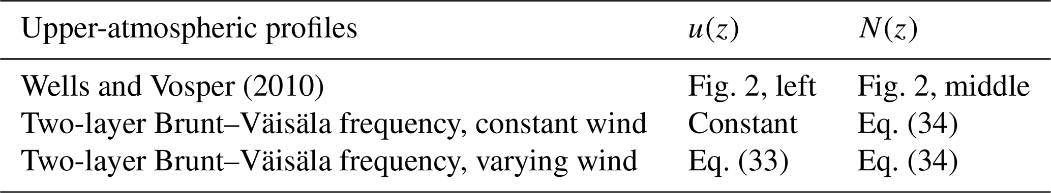
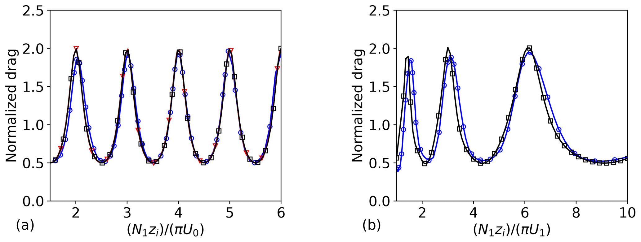
Figure 3Mountain wave drag on a small ridge with a two-layer Brunt–Väisäla frequency profile and constant background wind (a) and vertical wind shear (b), normalized by the drag for constant background profiles. The black lines with squares show our results, in which the wave drag is normalized with the drag for constant background wind u0 and stratification strength N1. The blue lines with circles show the results of Wells and Vosper (2010), and the red line with triangles in the left figure shows the results of Leutbecher (2001).
By using the piecewise-constant method developed in Sect. 3.2 to evaluate the stratification coefficients, the TLM can now take the variation in the stratification strength and wind speed with altitude into account. The impact of this non-uniformity on the interaction between gravity waves and wind farms is now analyzed in three ways. In Sect. 4.1, the impact of atmospheric profile variations on the stratification coefficients is analyzed by comparing for the idealized atmosphere used in Sect. 3.3 to the for a uniform upper atmosphere. The physical phenomenon causing the differences is identified as internal gravity-wave interference.
We further investigate how this influences the interaction between wind farms and gravity waves. To this end, Sect. 4.2 discusses an example case of ABL flow with a uniform upper atmosphere from Allaerts and Meyers (2019). By combining this case with the atmospheric profiles analyzed in previous sections, we investigate the effect of vertical variations in the atmospheric conditions on wind-farm–gravity-wave interaction. Finally, Sect. 4.3 presents a case study that estimates the overall impact of such variations by simulating 1 year of operation of the Belgian–Dutch offshore wind-farm cluster.
4.1 Stratification coefficients
To determine the effects of vertical non-uniformity on the pressure feedback of internal gravity waves, the stratification coefficients are calculated for the upper atmosphere used by Wells and Vosper (2010), shown in Fig. 2. The same grid as in Sect. 3.3 is used. The coefficients are calculated for both the original non-uniform and a uniform atmosphere. The latter was obtained by height-averaging the profiles of the velocity and the Brunt–Väisäla frequency, resulting in and . Figure 4 shows the results. Only is shown so that the important details are clearly visible. Since this is a 2D case, the transversal wavenumber l is zero. Comparing the two profiles for , it is clear that the vertical non-uniformity has a large impact on the stratification coefficients, with two peaks appearing at k≈0.36 and . We will now show that these changes in the profile of are caused by resonance in the free atmosphere.
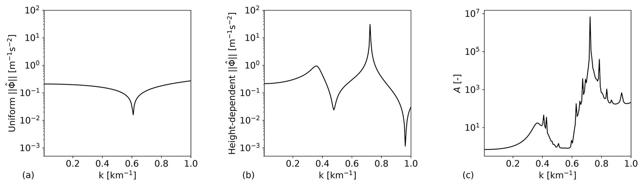
Figure 4The stratification coefficients for a uniform atmosphere with U=20.1 m s−1 and Ng=0.0113 s−1 (a), the stratification coefficients (b) and the gravity-wave resonance parameter (see Eq. 35) (c) for the vertical non-uniform atmosphere of Wells and Vosper (2010) used in Sect. 3.3. Only is shown so that the important details are clearly visible. Since this is a 2D case, the transversal wavenumber l is zero. Above , the gravity waves become evanescent within some sublayers, leading to oscillations in A that do not correspond to resonant behavior.
4.1.1 Internal wave resonance
While in a uniform atmosphere the wind farm can only trigger waves with an upwards group velocity, changes in the stratification and wind speed can cause waves to reflect. This allows both up- and downgoing waves to propagate throughout the atmosphere. As up- and downgoing internal gravity waves pass through each other, they interfere, potentially causing resonance. The resulting large wave amplitudes can drastically affect the pressure feedback of the waves (Teixeira, 2014). The ratio A between the mean wave energy at a given wavenumber for atmospheric profile with and without vertical variations is an effective measure for gravity-wave resonance as long as the waves are in the propagating regime (Gill, 1982). It is easily evaluated numerically using the following expression:
where e is the sum of the kinetic and potential energy densities (Gill, 1982):
For a sublayer in a piecewise-constant method, the integrals are straightforward to determine analytically, allowing A to be evaluated.
Figure 4 shows A for the atmosphere of Wells and Vosper (2010). It is clear that and A have a similar profile, with the same peaks occurring at and . Above , the gravity waves become evanescent within some sublayers, leading to oscillations in A that do not correspond to resonant behavior. Despite this, it is clear from the figure that the profiles of and A follow the same pattern, showing that the pressure feedback is largely determined by constructive and destructive interference of the internal gravity waves.
4.2 Gravity-wave ABL interaction
We investigate how variations in the wind and stability change the effects wind-farm operation has on the ABL flow by revising an example case used by Allaerts and Meyers (2019). By combining this case with the non-uniform upper atmosphere used in the previous sections, we identify the mesoscale flow perturbations triggered by the wind farm. One of these changes caused by the variations in the atmospheric conditions – the increase in the appearance and strength of resonant lee waves – is further analyzed.
4.2.1 Example cases
To analyze how the changes in the stratification coefficients impact the flows around wind farms, a flow case discussed earlier by Allaerts and Meyers (2019) is analyzed. This example case is simulated once with uniform upper atmospheres and once with the upper atmosphere discussed in Sects. 3.3 and 4.1.
The example case is set up to have a Froude number of Fr=1.1, with the Froude number given by Allaerts and Meyers (2019),
where is a velocity scale for the ABL (Allaerts and Meyers, 2019),
The Froude number represents the ratio of the advection terms in the momentum balance to the pressure gradient generated by the inversion waves (Durran, 1990). It is also a measure for the ratio of the wind speed to the velocity of inversion waves and therefore determines whether or not inversion waves can travel upstream from a stationary perturbation. This leads to the classification of flows as being either subcritical Fr<1, when inversion waves can affect the upstream flow, or supercritical Fr>1, when they cannot (Smith, 2010). Allaerts and Meyers (2019) analyzed two cases: one is subcritical, with Fr=0.9, while the other is supercritical, with Fr=1.1. Here, we focus on the supercritical case.
The example case is set up as follows. The mean flow in the two layers of the ABL is based on the analytical boundary layer model of Nieuwstadt (1983), with a cubic eddy viscosity profile and the Von Kármán constant κ=0.41 (Allaerts and Meyers, 2019). This model finds a velocity profile given a non-dimensional surface roughness length and non-dimensional boundary layer height . Combined with the stratification parameters g′ and Ng, this gives all the inputs required for the TLM. Allaerts and Meyers (2019) presume a conventionally neutral boundary layer, determining these stratification parameters with the non-dimensional groups and , where A=500 is an empirical constant (Csanady, 1974; Tjernstrom and Smedman, 1993). Since we want to analyze the impact vertical variations in the upper-atmospheric profile have on the flow, the original inputs used by Allaerts and Meyers (2019) are altered so that the upper atmosphere corresponds to the one analyzed in Sect. 4.1. The correct geostrophic wind and Brunt–Väisäla frequency are obtained by modifying u* and , respectively, and is changed so that the final result still has a Froude number of 1.1. H is increased so that h* and remain the same. The inputs are summarized in Table 2. Finally, the flow in the lower layer is aligned with the x direction.
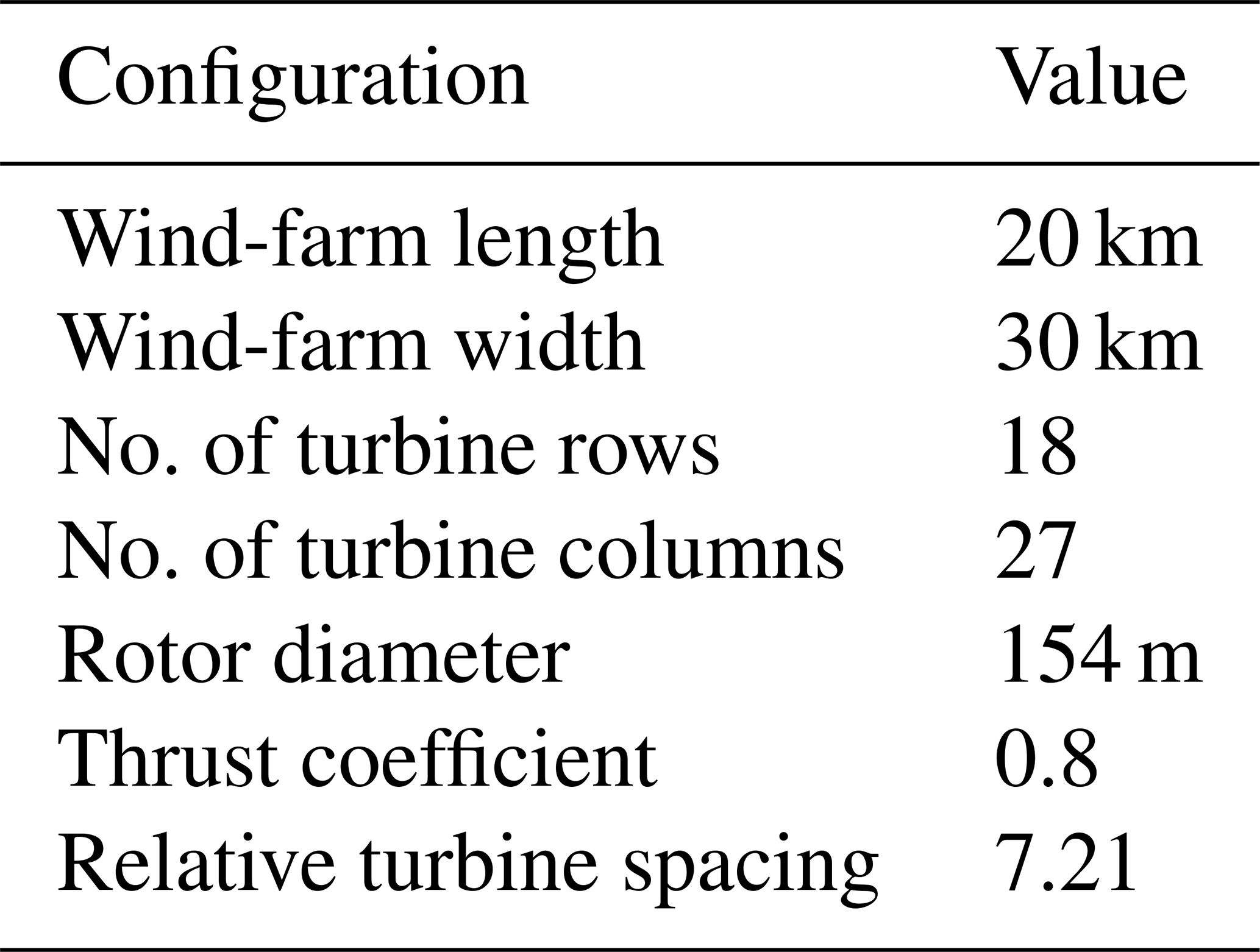
Table 3 gives an overview of the wind-farm configuration used by Allaerts and Meyers (2019), which is chosen to be comparable to the Belgian–Dutch wind-farm cluster in area and installed capacity. The turbines are placed in a staggered pattern with respect to the x direction, and the relative spacing is equal in the x and y directions. The simulations were performed on a 1000 km by 400 km grid, with 2000 by 800 grid points, which is the same as the grid spacing used in Sect. 3.3. For the vertically non-uniform simulation, the same vertical grid as in Sect. 3.3 and 4.1 is used.
Allaerts and Meyers (2019)Table 2Flow parameters of the flow case based on the one used by Allaerts and Meyers (2019). The atmospheric state corresponds to a PN of 1.1 and Fr of 1.1. For the vertically non-uniform case, the upper-atmospheric profiles of Wells and Vosper (2010), shown in Fig. 2, were used.
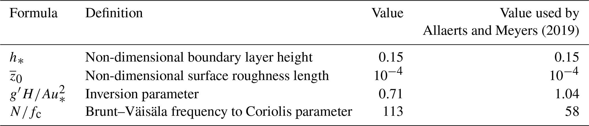
Table 3Wind-farm configuration of the reference flow cases, as analyzed by Allaerts and Meyers (2019).
The results of the uniform and non-uniform simulations are shown in Fig. 5. When comparing the results, it is clear that the mesoscale disturbances are much larger in the non-uniform case, with a stronger reduction in the farm inflow velocity. The farm's effects also spread out in the transversal directions as V-shaped patterns appear over large distances. Finally, the wind farm seems to trigger strong lee waves in its wake. These waves also appear in the reference case, although they are weaker there.
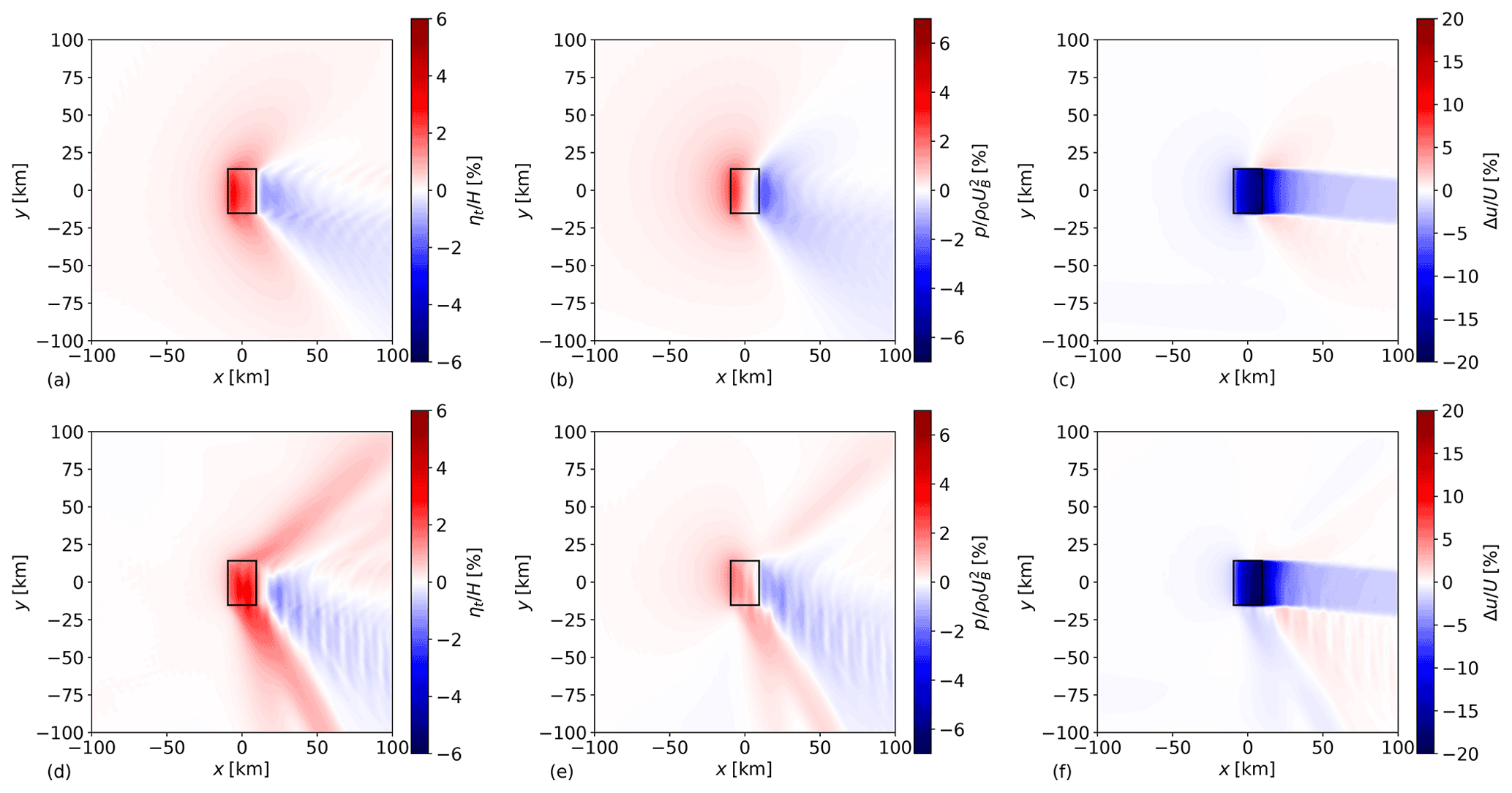
Figure 5Planform view of the inversion layer displacement ηt (a, d), pressure perturbation p′ (b, e), and velocity reduction in the lower layer u′ (c, f) in the reference uniform (a–c) and vertically varying (d–f) flow cases. The wind-farm region is indicated by the black rectangles.
4.2.2 Resonant lee waves in the ABL
We further analyze the lee waves that appear in Fig. 5 and show that they are associated in this case with internal wave reflection. We follow the ideas developed by Allaerts and Meyers (2019) by analyzing the equation for the total displacement ηt. When the wind in the ABL is aligned with the x axis , that equation corresponds to Allaerts and Meyers (2019):
where G is the geostrophic wind velocity. Furthermore, RHS1 and RHS2 are the right-hand sides of the Eqs. (6) and (7), respectively, and only depend on ηt through the turbulent viscosity, which is a relatively weak effect (Allaerts and Meyers, 2019). As discussed before, the Froude number Fr indicates the strength of the inversion waves. The second non-dimensional group PN governs the pressure induced by internal gravity waves and is given by
It reflects the fact that the pressure induced by a vertical displacement scales linearly with GNg in the hydrostatic regime. It is then clear that the left-hand side of Eq. (39) represents the forcing induced by flow advection and the corresponding gravity waves . These are balanced by the right-hand side of the equation, which represents the other terms in the momentum equations. If the advection terms and the pressure contributions from the gravity waves balance each other, the left-hand side of Eq. (39) becomes zero. This corresponds to a resonant state as ηt can be non-zero without external forcing, which explains the lee waves that appear in Fig. 5.
The left-hand side of Eq. (39) is easily expressed in Fourier components, leading to the definition of the two-dimensional lee-wave resonance parameter R:
where λ is the angle the horizontal wave vector makes with the k axis so that . The parameter R is a non-dimensional parameter indicating the flow's resistance to the occurrence of two-dimensional lee-wave resonance. If R=0, the pressure perturbations induced by ηt≠0 and the accompanying gravity waves balance the advection terms, and resonant lee waves appear. Equation (41), in combination with Eq. (4), shows that for uniform upper atmospheres, this type of resonance can only take place if the internal gravity waves are evanescent as has to be real for R to be zero. Physically, this corresponds to propagating waves not being able to trap the perturbation energy below the capping inversion (Vosper, 2004). In contrast, the wave reflection in vertically non-uniform atmospheres can cause part of the wave energy to be trapped by being reflected back. This corresponds to the stratification coefficients as given by Eq. (23) potentially having a real component, even in the propagating regime. The additional constraint found by Allaerts and Meyers (2019), that the flow has to be subcritical, is also not necessary when the waves can be reflected.
In order to apply this theory to the case from Sect. 4.2.1, Fig. 6 shows the wavenumber spectra for ηt and R. Figure 6 shows that low values of ||R|| correspond to high values of , indicating resonant lee waves in the ABL. The variations in wind and stability in the upper atmosphere can cause ||R|| to decrease several orders of magnitude in the propagating wave regime. This happens when the internal gravity-wave interference is destructive, which lowers the vertical energy flux of the waves considerably. This keeps the perturbation energy contained in the lower atmosphere, leading to low ||R||, which for uniform atmospheres only happens in the evanescent wave regime (Vosper, 2004; Allaerts and Meyers, 2019). In contrast, constructive interference can lead to very large values for , and thus for ||R||. Furthermore, when ||R||≫0, a large imbalance exists between the advection and pressure forces in the ABL. Changes in ABL height of the wavelengths at which this occurs cannot exist in an equilibrium system without external forcing. This is clearly visible in Fig. 6 as high values of ||R|| correspond to low values of . Internal gravity-wave resonance thus prohibits large displacements of the inversion layer at the wavelengths at which it occurs by creating large pressure gradients that cannot be counteracted by the flow acceleration.
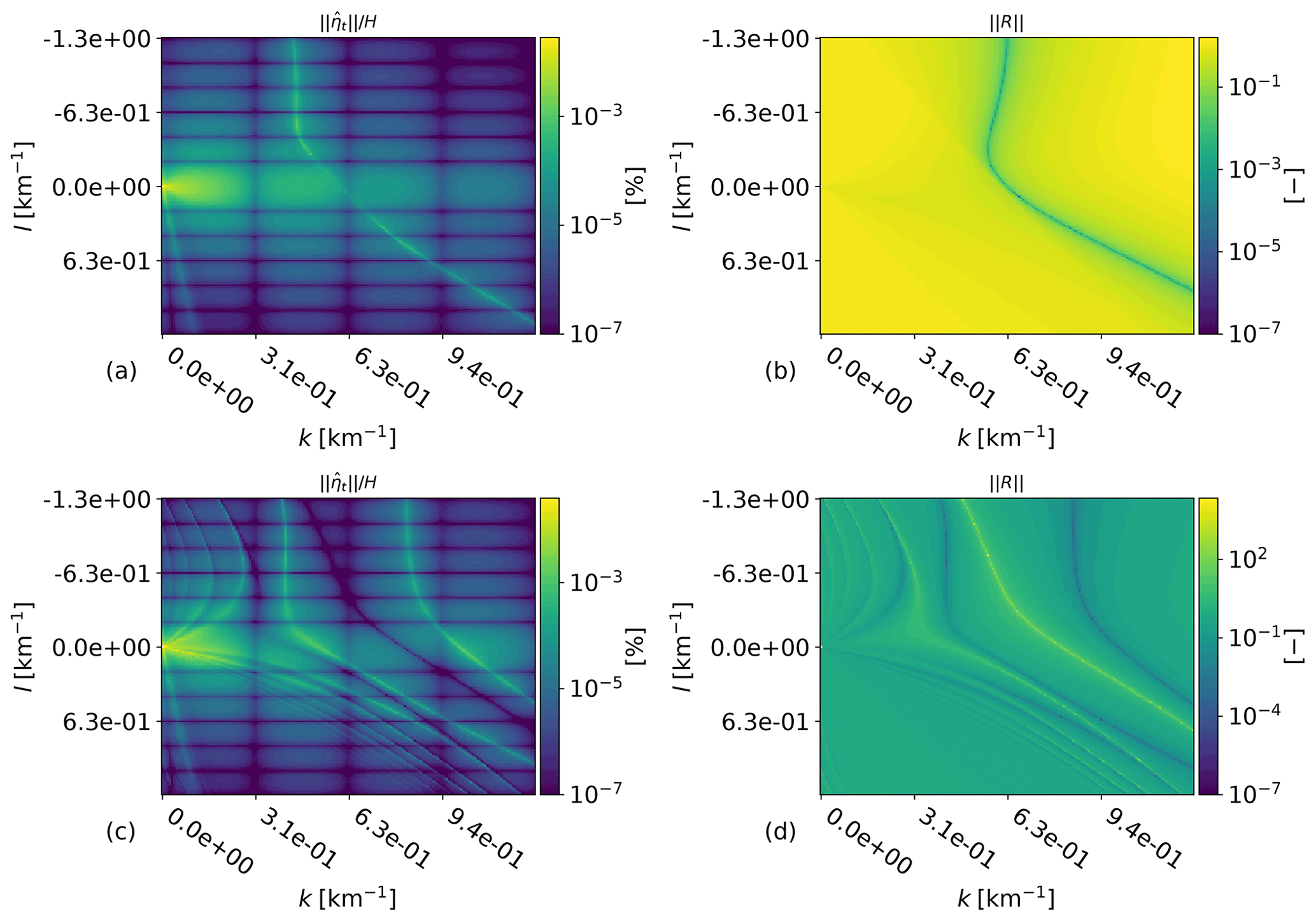
Figure 6 (a, c) and ||R|| (b, d) for the reference flow case with a uniform (a, b) and a non-uniform free atmosphere (c, d). Only the wavenumbers and are shown so that the important details are clearly visible. The left column shows parts of the Fourier transforms of the left column of Fig. 5.
While the above analysis explains how vertical variations in the atmospheric profile change the interaction between internal gravity waves and the ABL flow, it does not offer insight on how to predict the resulting impact on wind-farm performance. It is not clear what parameters could describe this. Extensive research has been done on internal gravity-wave resonance, with most of it focusing on flow around topographies. However, this has to be used with caution as the overall flow is then analyzed in the context of mountain wave drag, where the height displacement is given by the shape of the terrain (Teixeira, 2014). In contrast, the wind-farm forcing leads to this displacement through its interaction with the ABL. Additionally, it is itself influenced by the mesoscale effects it triggers, leading to an additional feedback loop. Parameters successfully describing internal wave resonance may therefore not be able to predict how vertical non-uniformity will impact the interaction with wind farms.
4.3 Overall impact
To determine the impact of varying wind speeds and stability on wind-farm energy production, we follow the approach of Allaerts et al. (2018) by simulating 1 year of wind-farm operation of the Belgian–Dutch wind-farm cluster. This analysis is performed with both uniform and non-uniform upper atmospheres, and the two are compared. The TLM input is based on ERA5 reanalysis data of the year 2016 from Hersbach et al. (2018), which are available at hourly frequency, resulting in 8784 flow cases. Like Allaerts et al. (2018), we use data from the grid point nearest to the wind-farm cluster, at 51.6∘ N, 3.0∘ E, and the same approach in determining the TLM input from the atmospheric data. We further assume that all turbines are DTU 10 MW reference turbines, a commonly analyzed model for which the power curve is readily available (Bortolotti et al., 2019), and place them within the same trapezoidal area as Allaerts et al. (2018). To ensure that we obtain the same total installed capacity of 3.8 GW, we scale the number of turbines and the turbine spacing from 475 and 7.36 to 380 and 8.23, respectively. The thrust coefficient of the turbines is set based on the height-averaged background velocity in the wind-farm layer of the TLM.
The simulations were performed on a 2000 by 2000 grid, on a 1000 km by 1000 km domain, the same grid density as in the previous sections. Variations in the atmospheric profiles were taken into account up to the tropopause. Within the troposphere, the potential temperature and velocity profiles were modeled as first- and third-order splines, respectively, through the ERA5 data points, around which the sublayers were spaced as well, resulting in 30 to 50 sublayers for each case. The tropopause altitude and the stratification in the stratosphere were determined with a two-line, piecewise-linear regression fit on the temperature profiles between the ABL height and 15 km. The velocity in the stratosphere was then determined by height-averaging the profile from the tropopause up to 15 km. As an example, Fig. 7 shows the profiles of θ, u, and v for the upper atmosphere at 00:00 GMT on 1 May 2016.
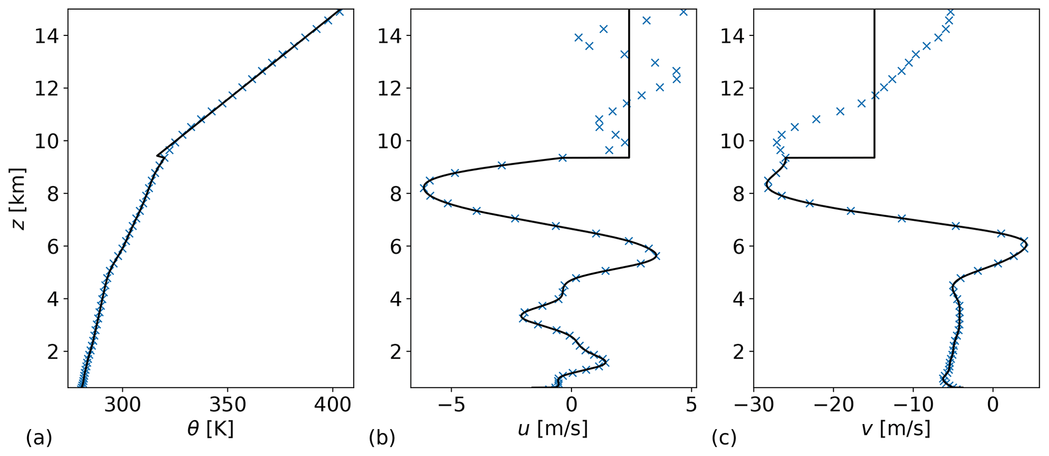
Figure 7The atmospheric profiles of potential temperature (a), velocity in the x (b) and y direction (c). The blue crosses are the ERA5 data, and the black lines are the inputs to the TLM, showing the piecewise-constant approximation made in the discretization.
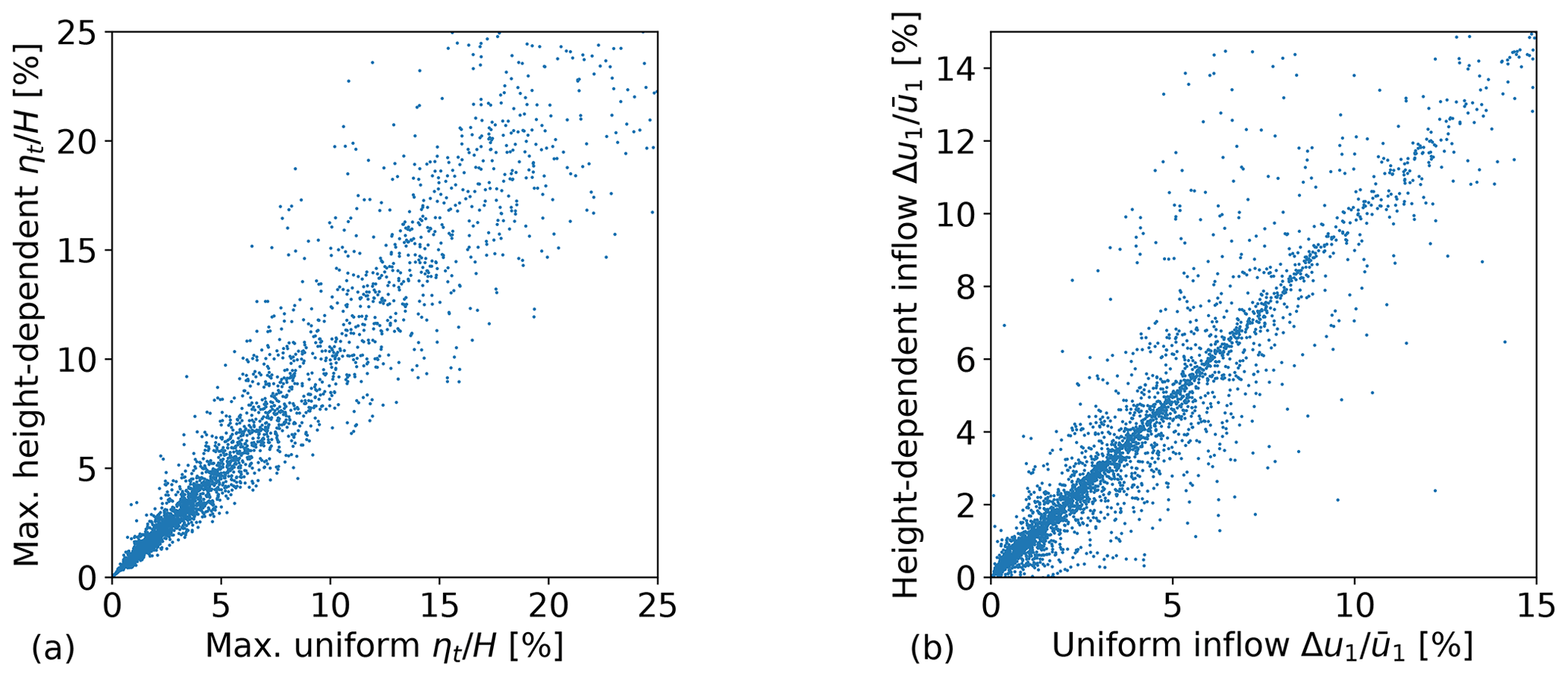
Figure 8The maximum capping inversion displacement (a) and the inflow velocity perturbation (b) for all analyzed cases with both uniform (x axis) and non-uniform (y axis) upper atmospheres.
From the 8746 cases, we only use those where the atmosphere is statically stable at every altitude in the free atmosphere. Additionally, the cases without capping inversion, (cf. earlier discussion following Eq. 10 in Sect. 2.2) or with a capping inversion situated lower than twice the turbine hub height were left out, leaving 3890 cases. This filtering was necessary as for the removed cases the assumptions made in the derivation of the model are not valid, as discussed in Sect. 2.2. The results of the simulations are shown in Fig. 8 and summarized in Table 4. On average, the difference between the results with non-uniform and uniform upper atmospheres is small. Despite this however, the impact on individual cases is often significant. In 16.6 % of the analyzed cases, the difference between the uniform and the non-uniform inflow perturbation was more than 30 % of the uniform perturbation case. We therefore conclude that vertical variations in the upper-atmospheric profiles are important to take into account when analyzing individual flow cases.
Table 4Average perturbations over all the analyzed flow cases for both uniform and non-uniform upper atmospheres.

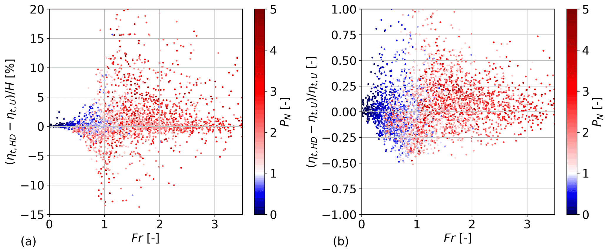
Figure 9The difference between the maximum capping inversion displacements in the non-uniform and uniform simulations as normalized by the ABL height (a) and the displacement in the uniform simulation (b), plotted against the parameters Fr and PN. The lack of a clear trend in both figures indicates that Fr and PN are not related to the impact of the vertical non-uniformity.
Figure 9 shows that the differences between the simulations seem to be independent from parameters that were good predictors of the TLM's behavior in previous studies, such as Fr and PN. We also investigated parameters that were found to correlate well with mountain wave drag in vertically non-uniform atmospheres, such as c1 as found by Klemp and Lilly (1975) (Eq. 16), but could not identify a meaningful correlation in our case. Directional shear effects, such as those investigated by Teixeira et al. (2008), might explain the discrepancy.
The goal of this study was to extend the applicability of a wind-farm gravity-wave model to vertically non-uniform free atmospheres. This was done by changing the expressions for the stratification coefficients to results derived from the internal wave equation for general stratified flows. By applying the well-known piecewise method with large numbers of sublayers, general stratification and velocity profiles can be incorporated into the model.
The effects of the variations in background wind and stability were studied by analyzing how free-atmospheric wave reflection influences the wave pressure feedback, the ABL flow, and overall wind-farm performance. Firstly, the stratification coefficients for the idealized atmosphere used by Wells and Vosper (2010) were compared to those for a uniform atmosphere based on it. The differences were found to be caused by constructive and destructive interference of the internal gravity waves in the free atmosphere. In a second step, this vertically non-uniform atmosphere was combined with a flow case used by Allaerts and Meyers (2019). An analysis of the appearance of resonant lee waves led to a qualitative understanding of the vertical non-uniformity's effects on the interaction between gravity waves and the ABL flow. Due to destructive internal wave interference, resonant lee waves can appear. On the other hand, internal gravity-wave resonance dampens inversion layer displacement for the wavelengths at which it occurs.
Finally, the extended TLM was used to simulate 1 year of operation of the Belgian–Dutch wind-farm cluster, repeating a similar analysis by Allaerts et al. (2018), in order to determine overall impact of variations in the atmospheric profiles on the interaction between the ABL flow and the gravity waves to be determined. While this impact was found to be small when averaged out over all flow cases, for individual flow cases it is often of the same order of magnitude as the total flow perturbation. In 16.6 % of the analyzed flows, the variations in the atmospheric profiles caused a relative difference in the upstream velocity reduction of more than 30 %. It is unclear how the effect of this non-uniformity for individual flow cases can be predicted since it does not simply scale with Fr or PN.
The results of this study show that vertical atmospheric non-uniformity could play a major role in the interaction between wind farms and gravity waves. This suggests that variations with altitude of the free atmosphere's wind and stability should be taken into account when simulating wind-farm operation in specific atmospheric conditions and may be important for the optimization of turbine control in the future (see, e.g., Lanzilao and Meyers, 2021b). In the future, we foresee further improvements of the TLM, among others, including hydrodynamic effects in the boundary layer and upgrading the wake model to include the improved wake merging model by Lanzilao and Meyers (2021a). Next to that, we plan further validation against detailed large-eddy simulations (similar to Allaerts and Meyers, 2019) and data from operational wind farms.
Adding more sublayers leads to a better approximation of the actual profiles of atmospheric variables. This would then also result in a better approximation of W(z). To estimate the rate of convergence, z* is defined as the altitude where . If n is sufficiently large, such an altitude exists in each sublayer. The error can then be written as a Taylor expansion around z*:
Using the above result, the change in error over the jth sublayer ΔjE can be written as
Because , with ΔjH the thickness of the jth sublayer, a maximum value for |ΔEj| is given by
If somewhere in the sublayer, substituting a Taylor expansion for m2 then directly leads to
From this analysis, it is clear that the piecewise-constant method has the best result when the distance to z* is minimized for all z. Therefore, when approximating a general continuously varying atmosphere, sublayers should be evenly spaced, and the atmospheric state should be evaluated halfway through each sublayer when calculating . In that case, the maximum error can be expected to scale with n|ΔjE| and , resulting in a second-order rate of convergence, as also found with a different derivation by Pütz et al. (2019). This is confirmed by comparison with a finite-difference solver.
It is notable that the above derivation is not limited to piecewise-constant methods but is valid for general piecewise methods. Therefore, as long as is not set up so that , the convergence rate will remain second-order. For example, we also developed a piecewise-linear methods using Airy functions instead of exponential functions that did not outperform the piecewise-constant one. This is because when linearly approximating a general function m2(z), and W(z*) will still not coincide. As a result, there is no improvement for general atmospheric profiles.
The code used for the simulations and the raw data of the simulation results can be provided by contacting the corresponding author. An open-source version of the code is planned to be released by the end of the year. The code used for the simulations is written in Python.
KD, LL, NvL, and JM jointly derived how to apply the piecewise method to the TLM and set up the verification and simulation studies. KD performed code implementations and carried out the simulations. SJ provided the optimization tool used to determine the altitude of the tropopause. KD, LL, SJ, NvL, and JM jointly wrote the manuscript.
At least one of the (co-)authors is a member of the editorial board of Wind Energy Science. The peer-review process was guided by an independent editor, and the authors also have no other competing interests to declare.
Publisher’s note: Copernicus Publications remains neutral with regard to jurisdictional claims in published maps and institutional affiliations.
The computational resources and services in this work were provided by the VSC (Flemish Supercomputer Center), funded by the Research Foundation Flanders (FWO) and the Flemish Government department EWI. The work of Hersbach et al. (2018) was downloaded from the Copernicus Climate Change Service (C3S) Climate Data Store. The results contain modified Copernicus Climate Change Service information from 2020. Neither the European Commission nor ECMWF is responsible for any use that may be made of the Copernicus information or data it contains.
This research has been supported by the Energy Transition Fund of the Belgian Federal Public Service for Economy, SMEs, and Energy (FOD Economie, K.M.O., Middenstand en Energie).
This paper was edited by Andrea Hahmann and reviewed by two anonymous referees.
Allaerts, D. and Meyers, J.: Boundary-layer development and gravity waves in conventionally neutral wind farms, J. Fluid Mech., 814, 95–130, https://doi.org/10.1017/jfm.2017.11, 2017. a
Allaerts, D. and Meyers, J.: Sensitivity and feedback of wind-farm-induced gravity waves, J. Fluid Mech., 862, 990–1028, https://doi.org/10.1017/jfm.2018.969, 2019. a, b, c, d, e, f, g, h, i, j, k, l, m, n, o, p, q, r, s, t, u, v, w, x, y, z, aa, ab, ac, ad
Allaerts, D., Broucke, S. V., Van Lipzig, N., and Meyers, J.: Annual impact of wind-farm gravity waves on the Belgian-Dutch offshore wind-farm cluster, J. Phys.-Conf. Ser., 1037, 072006, https://doi.org/10.1088/1742-6596/1037/7/072006, 2018. a, b, c, d
Baines, P. G.: Topographic effects in stratified flows, Cambridge monographs on mechanics, Cambridge University Press, ISBN 0-521-62923-3, 1998. a, b, c, d, e, f, g
Bastankhah, M. and Porté-Agel, F.: A new analytical model for wind-turbine wakes, Renew. Energ., 70, 116–123, https://doi.org/10.1016/j.renene.2014.01.002, 2014. a
Bleeg, J., Purcell, M., Ruisi, R., and Traiger, E.: Wind farm blockage and the consequences of neglecting its impact on energy production, Energies, 11, 1609, https://doi.org/10.3390/en11061609, 2018. a
Bortolotti, P., Tarres, H. C., Dykes, K. L., Merz, K., Sethuraman, L., Verelst, D., and Zahle, F.: IEA Wind TCP Task 37: Systems Engineering in Wind Energy – WP2.1 Reference Wind Turbines, technical report, https://doi.org/10.2172/1529216, 2019. a
Csanady, G. T.: Equilibrium theory of the planetary boundary layer with an inversion lid, Bound.-Lay. Meteorol., 6, 63–79, https://doi.org/10.1007/BF00232477, 1974. a
Durran, D. R.: Mountain Waves and Downslope Winds, American Meteorological Society, Boston, MA, 59–81, https://doi.org/10.1007/978-1-935704-25-6_4, 1990. a, b
Gill, A. E.: Atmosphere-Ocean Dynamics, International geophysics series 30, edited by: Donn, W. L., Academic Press, Inc., San Diego, USA, ISBN 0-12-283522-0, 1982. a, b, c, d, e, f, g, h, i, j
Gossard, E. E. and Hooke, W. H.: Waves in the atmosphere : atmospheric infrasound and gravity waves – their generation and propagation, Developments in atmospheric science 2, Elsevier Scientific Publishing Company, ISBN 0-444-41196-8, 1975. a, b, c, d, e, f
Hersbach, H., Bell, B., Berrisford, P., Biavati, G., Horányi, A., Muñoz Sabater, J., Nicolas, J., Peubey, C., Radu, R., Rozum, I., Schepers, D., Simmons, A., Soci, C., Dee, D., and Thépaut, J.-N.: ERA5 hourly data on pressure levels from 1979 to present, Copernicus Climate Change Service (C3S) Climate Data Store (CDS) [data set], https://doi.org/10.24381/cds.bd0915c6, 2018. a, b
Klemp, J. B. and Lilly, D. K.: Dynamics of Wave-Induced Downslope Winds, J. Atmos. Sci., 32, 320–339, https://doi.org/10.1175/1520-0469(1975)032<0320:TDOWID>2.0.CO;2, 1975. a, b, c
Lam, S. K., Pitrou, A., and Seibert, S.: Numba: A LLVM-Based Python JIT Compiler, in: Proceedings of the Second Workshop on the LLVM Compiler Infrastructure in HPC, LLVM '15, Association for Computing Machinery, New York, NY, USA, https://doi.org/10.1145/2833157.2833162, 2015. a
Lanzilao, L. and Meyers, J.: A new wake-merging method for wind-farm power prediction in the presence of heterogeneous background velocity fields, Wind Energy, 25, 237–259, https://doi.org/10.1002/we.2669, 2021a. a
Lanzilao, L. and Meyers, J.: Set-point optimization in wind farms to mitigate effects of flow blockage induced by atmospheric gravity waves, Wind Energ. Sci., 6, 247–271, https://doi.org/10.5194/wes-6-247-2021, 2021b. a, b
Leutbecher, M.: Surface pressure drag for hydrostatic two-layer flow over axisymmetric mountains, J. Atmos. Sci., 58, 797–807, https://doi.org/10.1175/1520-0469(2001)058<0797:SPDFHT>2.0.CO;2, 2001. a, b, c
Nappo, C. J.: An introduction to atmospheric gravity waves, Academic Press, ISBN 9780123852243, 2012. a, b
Niayifar, A. and Porté-Agel, F.: Analytical modeling of wind farms: A new approach for power prediction, Energies, 9, 1–13, https://doi.org/10.3390/en9090741, 2016. a
Nieuwstadt, F. T. M.: On the solution of the stationary, baroclinic Ekman-layer equations with a finite boundary-layer height, Boundary-Layer Meteorology, 26, 377–390, https://doi.org/10.1007/BF00119534, 1983. a
Pütz, C., Schlutow, M., and Klein, R.: Initiation of ray tracing models: evolution of small-amplitude gravity wave packets in non-uniform background, Theor. Comp. Fluid Dyn., 33, 509–535, https://doi.org/10.1007/s00162-019-00504-z, 2019. a, b, c, d, e, f, g
Sachsperger, J., Serafin, S., and Grubišić, V.: Lee waves on the boundary-layer inversion and their dependence on free-atmospheric stability, Front. Earth Sci., 3, 1–11, https://doi.org/10.3389/feart.2015.00070, 2015. a
Salomons, E. M.: Computational Atmospheric Acoustics, Springer, https://doi.org/10.1007/978-94-010-0660-6, 2001. a
Smith, R. B.: Linear theory of stratified hydrostatic flow past an isolated mountain., Tellus, 32, 348–364, https://doi.org/10.3402/tellusa.v32i4.10590, 1980. a
Smith, R. B.: Interacting mountain waves and boundary layers, J. Atmos. Sci., 64, 594–607, https://doi.org/10.1175/JAS3836.1, 2007. a
Smith, R. B.: Gravity wave effects on wind farm efficiency, Wind Energy, 13, 449–458, https://doi.org/10.1002/we.366, 2010. a, b, c, d, e, f, g, h
Smith, R. B., Skubis, S., Doyle, J. D., Broad, A. S., Kiemle, C., and Volkert, H.: Mountain waves over Mont Blanc: Influence of a stagnant boundary layer, J. Atmos. Sci., 59, 2073–2092, https://doi.org/10.1175/1520-0469(2002)059<2073:MWOMBI>2.0.CO;2, 2002. a, b, c, d
Teixeira, M. A.: The physics of orographic gravity wave drag, AIP Conf. Proc., 2, 1–24, https://doi.org/10.3389/fphy.2014.00043, 2014. a, b, c, d, e, f
Teixeira, M. A. and Argaín, J. L.: The dependence of mountain wave reflection on the abruptness of atmospheric profile variations, Q. J. Roy. Meteor. Soc., 146, 1685–1701, https://doi.org/10.1002/qj.3760, 2020. a
Teixeira, M. A. C., Miranda, P. M. A., and Argaín, J. L.: Mountain Waves in Two-Layer Sheared Flows: Critical-Level Effects, Wave Reflection, and Drag Enhancement, J. Atmos. Sci., 65, 1912–1926, https://doi.org/10.1175/2007JAS2577.1, 2008. a
Teixeira, M. A., Argaín, J., and Miranda, P.: Drag produced by trapped lee waves and propagating mountain waves in a two-layer atmosphere, Q. J. Roy. Meteor. Soc., 139, 964–981, https://doi.org/10.1002/qj.2008, 2013. a, b
Tjernstrom, M. and Smedman, A. S.: The vertical turbulence structure of the coastal marine atmospheric boundary layer, J. Geophys. Res., 98, 4809–4826, https://doi.org/10.1029/92JC02610, 1993. a
Tolstoy, I.: Wave Propagation, International Series in the Earth & Planetary Sciences, McGraw-Hill, ISBN 0-07-064944-8, 1973. a, b, c, d
Virtanen, P., Gommers, R., Oliphant, T. E., Haberland, M., Reddy, T., Cournapeau, D., Burovski, E., Peterson, P., Weckesser, W., Bright, J., van der Walt, S. J., Brett, M., Wilson, J., Millman, K. J., Mayorov, N., Nelson, A. R. J., Jones, E., Kern, R., Larson, E., Carey, C. J., Polat, İ., Feng, Y., Moore, E. W., VanderPlas, J., Laxalde, D., Perktold, J., Cimrman, R., Henriksen, I., Quintero, E. A., Harris, C. R., Archibald, A. M., Ribeiro, A. H., Pedregosa, F., van Mulbregt, P., and SciPy 1.0 Contributors: SciPy 1.0: Fundamental Algorithms for Scientific Computing in Python, Nat. Methods, 17, 261–272, https://doi.org/10.1038/s41592-019-0686-2, 2020. a
Vosper, S. B.: Inversion effects on mountain lee waves, Q. J. Roy. Meteor. Soc., 130, 1723–1748, https://doi.org/10.1256/qj.03.63, 2004. a, b, c, d
Wells, H. and Vosper, S. B.: The accuracy of linear theory for predicting mountain-wave drag: Implications for parametrization schemes, Q. J. Roy. Meteor. Soc., 136, 429–441, https://doi.org/10.1002/qj.578, 2010. a, b, c, d, e, f, g, h, i, j, k, l, m, n, o, p, q
WindEurope: Wind energy in Europe: Outlook to 2022, Annual report from 2018, 2018. a
Yu, C. L. and Teixeira, M. A.: Impact of non-hydrostatic effects and trapped lee waves on mountain-wave drag in directionally sheared flow, Q. J. Roy. Meteor. Soc., 141, 1572–1585, https://doi.org/10.1002/qj.2459, 2015. a
- Abstract
- Introduction
- Gravity-wave interaction with wind farms
- Extension to vertically non-uniform free atmospheres
- Effects of vertically varying wind and stability
- Conclusions
- Appendix A: Convergence analysis
- Code and data availability
- Author contributions
- Competing interests
- Disclaimer
- Acknowledgements
- Financial support
- Review statement
- References