High-fidelity aeroelastic analyses of wind turbines in complex terrain: fluid–structure interaction and aerodynamic modeling

This paper shows high-fidelity fluid–structure interaction (FSI) studies applied to the research wind turbine of the WINSENT (Wind Science and Engineering in Complex Terrain) project. In this project, two research wind turbines are going to be erected in the south of Germany in the WindForS complex-terrain test field. The FSI is obtained by coupling the CFD URANS–DES code FLOWer and the multiphysics FEM solver Kratos Multiphysics, in which both beam and shell structural elements can be chosen to model the turbine. The two codes are coupled in both an explicit and an implicit way. The different modeling approaches strongly differ with respect to computational resources, and therefore the advantages of their higher accuracy must be correlated with the respective additional computational costs. The presented FSI coupling method has been applied firstly to a single-blade model of the turbine under standard uniform inflow conditions. It could be concluded that for such a small turbine, in uniform conditions a beam model is sufficient to correctly build the blade deformations. Afterwards, the aerodynamic complexity has been increased considering the full turbine with turbulent inflow conditions generated from real field data, in both flat and complex terrains. It is shown that in these cases a higher structural fidelity is necessary. The effects of aeroelasticity are then shown on the phase-averaged blade loads, showing that using the same inflow turbulence, a flat terrain is mostly influenced by the shear, while the complex terrain is mostly affected by low-velocity structures generated by the forest. Finally, the impact of aeroelasticity and turbulence on the damage equivalent loading (DEL) is discussed, showing that flexibility reduces the DEL in the case of turbulent inflow, acting as a damper that breaks larger cycles into smaller ones.

1 Introduction

According to Renewable Energy Statistics 2020 of the International Renewable Energy Agency (IRENA, 2021), the global installed wind power capacity has increased by a factor of almost 83 in the last 20 years, from around 7.5 GW in 1997 to around 622 GW in 2019. In 2018 wind energy represented around 19 % of the total electricity produced by renewables worldwide. This makes wind energy the highest growing renewable power technology nowadays. One of the reasons for its extreme development is strong investment in the research of new materials and construction techniques in order to reach larger and lighter rotor designs. According to IEA, 2021, the global average cost of electricity from onshore fell from USD 76 per megawatt hour in 2016 to USD 53 per megawatt hour in 2019, and it is expected to decrease 15 % during 2020–2025, expanding the market of bankable projects to low-wind-speed areas and complex terrains. A complex terrain is a terrain where topology and roughness have a significant impact on the wind in the atmospheric boundary layer (ABL). For this reason, differently from an offshore wind turbine that is characterized by high inflow velocities and low turbulence intensity (TI), a complex terrain has exactly the opposite attributes. This makes it difficult to estimate the wind potential and consequently the performances of the installed wind turbine. Therefore high fidelity is necessary to simulate the site-specific wind field and turbulence. It needs to be considered that the produced power of a turbine is proportional to the cube of the velocity, and therefore a 3 % error in the velocity leads to a 9 % error in the power calculation. Those effects can already be mapped using RANS methods as in Brodeur and Masson (2008). On the other hand, higher-fidelity models such as hybrid RANS–large eddy simulation (LES) are needed to catch the effects on the turbulence of smaller vortices from the ground (Bechmann and Sørensen, 2010). The applicability of detached delayed eddy simulations (DDESs) for wind turbines was shown by Weihing et al. (2018), while DDES investigations of a complex terrain have been conducted by Schulz et al. (2016), focusing on the performance of the turbine. A widely studied complex terrain is the double ridge in Perdigão in Portugal, where a single turbine has been erected with consequent measurements campaigns in 2017 (Fernando et al., 2019). On the other hand, the increase in rotor sizes with the consequent necessity of slender blades makes it impossible to neglect aeroelastic effects, and that is why aeroelastic models based on different fidelity levels have been developed within the research community. DTU, for example, widely uses the fluid–structure interaction (FSI) coupling developed by Heinz et al. (2013) and known as HAWC2CFD between the CFD solver EllipSys3D (Sørensen, 1995; Michelsen, 1992) and the finite-element multibody serial solver HAWC2 (Larsen and Hansen, 2007). Heinz et al. (2016a) used it on the NREL 5 MW rotor and compared it to blade element momentum (BEM)-based calculations using HAWC2, too. Most discrepancies were shown when the turbine was at a standstill, although good agreement was found in uniform and yawed conditions. Li et al. (2017) used the same turbine, adding a turbulent inflow synthetically generated by the use of a Mann box, a multibody drivetrain and a control system. They showed that an active pitching control led to a more uniformly distributed wake even in turbulent inflow conditions, in comparison to a stall-regulated study. The same coupling has been used in Heinz et al. (2016b) to perform studies on vortex-induced vibrations (VIVs). In this case a single-blade model of the DTU 10 MW wind turbine has been take into account, finding that the conditions triggering VIVs are an angle of attack (AOA) of around 90^∘ and a flow inclination between 20 and 55^∘. Horcas et al. (2020) continued their work analyzing the effect of different tip configurations on the VIV phenomenon for the same turbine. Recently, the HAWC2CFD FSI coupling has been used by Grinderslev et al. (2021) to aeroelastically investigate the DANAERO 2.3 MW rotor using a new turbulence model, combining the Deardorff LES model for atmospheric flow with an improved detached delayed eddy simulation (IDDES) model for the near-rotor area. The authors found that for such stiff turbines, flexibility has only a marginal effect, while the loading was strongly affected by the inflow turbulence, underlining the importance of its modeling.

Santo et al. (2020a) used an FSI coupling between a CFD URANS model in Ansys and a structural shell model in Abaqus to analyze the effects of tilt, yaw, tower shadow and wind shear. The authors found that yaw leads to a lower deflection but a higher yaw moment on the hub. In Santo et al. (2020b), gusts were introduced showing that in the case considered, flow separation was occurring working as a passive load control.

Streiner et al. (2008), Meister (2015) and Klein et al. (2018) worked sequentially on an FSI coupling between the CFD code FLOWer and the multibody simulation (MBS) commercial solver SIMPACK. In Klein et al. (2018), the NREL 5 MW wind turbine was simulated, including the drivetrain torsion, the foundation flexibility and the controller for variation in revolutions per minute (rpm) and pitch angle, examining thereby the origin of low-frequency noise sources and seismic excitation. The same coupling was then used in Guma et al. (2021) to simulate the DANAERO wind turbine in both uniform and turbulent conditions, these ones synthetically generated by the use of a Mann box (Mann, 1994). Results in uniform inflow were compared to a consistent low-fidelity model, and analysis on the effects on the damage equivalent loading (DEL) have been carried out. Here it was demonstrated that for the specific inflow case, the deformations have only a marginal influence on the DEL, which is shown to be more affected by the inflow turbulence fluctuations. The same CFD solver was coupled by Sayed et al. (2016) to the CSD solver Carat$++$ and applied to a blade-only model of the DTU 10 MW generic rotor under uniform inflow conditions. Both beam and shell elements have been applied, showing that an evident error is made when geometric nonlinearities are not taken into account.

Dose et al. (2018) coupled the flow solver OpenFOAM to the FEM-based beam solver BeamFOAM to perform simulations of the NREL 5 MW rotor, showing that aeroelasticity is particularly important when a yaw misalignment is taken into account. The same rotor was adopted by Yu and Kwon (2014) using a loose CFD–CSD coupling with an incompressible CFD solver and nonlinear Euler–Bernoulli beam elements for the structure. The communication in this case was only once per revolution. The same turbine was also used by Bazilevs et al. (2011, 2012) by means of FSI between a low-order arbitrary Lagrangian–Eulerian variational multiscale (ALE-VMS) flow solver and a non-uniform rational basis spline (NURBS)-based structural solver. An isogeometric analysis (IGA) has been used in this case, which integrates FEM into the CAD tool so that no geometric approximation is needed. This increases its accuracy and simplicity, especially for form optimization chains.

Within the scope of the present study, a highly accurate CFD–FEM coupling has been built and a model has been created for a small research wind turbine to be erected in a complex-terrain location in the south of Germany. Two different structural models and coupling algorithms have been used to determine their impact in different inflow configurations. Starting from a single-blade model and a full model of the turbine in uniform standard conditions and moving to the turbulent inflow conditions in both flat and complex terrain, the difference in deformations, wake shape, loads and fatigue are analyzed. Considering the strong variation in computational costs within the different configurations, it is of particular interest to determine the respective fidelity requirements. Section 2 describes the methodology, from the CFD to the CSD models and the construction of the coupling. Section 3 shows the results firstly for a single-blade model and then for the full turbine, focusing on the wake shape, the impact of the terrain and effects on the fatigue loading.

2 Methodology

2.1 WINSENT research wind turbine

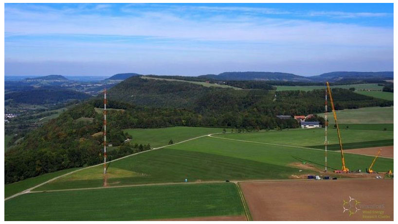
The project WINSENT (Wind Science and Engineering in Complex Terrain) is a German project (WindForS, 2016) involving different universities and research institutions in the south of Germany. The site is located in Stöttener Berg, a complex-terrain location in the Swabian Alb (Fig. 1), where two research wind turbines will be erected. These will be pitch-regulated and will each have around a 50 m diameter, a 70 m hub height, a tilt angle of 4^∘, a cone angle of 2.5^∘ and a rated power of around 750 kW, with a rated inflow velocity of 11 m s⁻¹ and a rotor speed of 26.5 rpm. They will be equipped with measuring technology for the validation of both high (presented in this work) and low fidelity. A computational chain has been developed within the project, starting from mesoscale simulations up to high-fidelity FSI calculations in the near field around the turbine. A large variety of measurement equipment has been used to characterize the local site-specific wind field, such as unmanned aerial systems (UASs), lidar instruments and met masts with ultrasonic anemometers. This has allowed us to validate CFD terrain calculations with the data from the met masts as prescribed in Letzgus et al. (2020).

Figure 1 WindForS test field in Stöttener Berg (from Testfield, 2017) with focus on the two met masts.

This paper focuses on the final part of the simulation chain, in which the CFD terrain calculations are used as inflow conditions to analyze the aeroelastic effects on the research wind turbine by means of high-fidelity FSI.

Starting from the CAD file provided and material properties, models with different degrees of fidelity have been built.

2.1.1 CFD model and inflow conditions

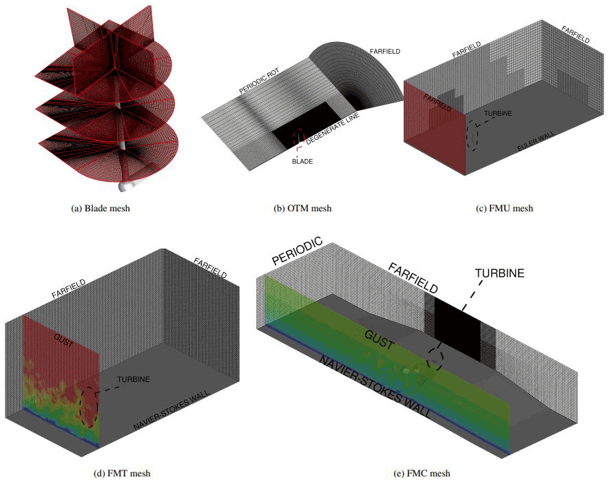
The CFD code used within this study is FLOWer (Raddatz, 2009). This was originally developed at the German Aerospace Centre (DLR), and for many years it has been expanded at the Institute of Aerodynamics and Gas Dynamics for helicopter and wind turbine purposes. It is a finite-volume URANS and DES code, using structured meshes. Both second-order central-cell-centered (Jameson et al., 1981) and fifth-order-weighted essentially non-oscillatory (Kowarsch et al., 2013) spatial discretization schemes are available. The second type is utilized in the background meshes in this study to reduce the turbulence dissipation. A dual-time-stepping integration scheme is applied, in which the number of inner iterations of a time step t is dependent on how close a guessed solution is to the final value, based on a prescribed tolerance. An artificial five-stage Runge–Kutta scheme is used as a time-stepping scheme. Up to three levels of multigrid can be utilized to accelerate convergence, although a complex-terrain mesh is not suited for this. Single meshes for each component need to be independently generated and then combined by means of the chimera technique. The shear-stress-transport (SST) k–ω model according to Menter (1993) with a fully turbulent boundary layer is used for the simulations in this study. URANS has been used here for all cases with uniform inflow conditions, while DDES has been activated when turbulence was involved. In this way the turbulence propagation is resolved by LES, while the areas close to the wall and therefore the boundary layer are resolved by URANS. Bangga et al. (2017) showed DDES combined with this turbulence model had the most stable and best results compared to measured data. The CFD model of the turbine has been built starting from the provided CAD files. A “watertight” outer surface has been extracted, and meshing has been performed with use of both Pointwise and in-house scripts. All components have been meshed ensuring $y^{+}\le \mathrm{1}$ of the wall-nearest cell. Mesh refinement studies of the blade have been done in Guma et al. (2018) and Schäffler (2019). According to these studies, different mesh properties, characteristics and sizes have been tested to optimize the profile and the trailing- and leading-edge resolutions, as well as the wake and pinion areas. Different time steps and numbers of iterations have been also tested, although always at rated conditions. For this reason the second-cheapest number of cells has been then chosen in order to remain conservative and in line with other similar works performed with the same code. The blade mesh in Fig. 2a has been generated with the following properties:

Figure 2 Details of the meshes.

• CH mesh,

• 193 sections over the blade with 257 points over each profile,

• 32 cells in the boundary layer with a growth rate of 1.11,

• a total of around 12 million cells for each blade.

Three different CFD models of the turbine have been built with the following characteristics and abbreviations:

• a one-third model with only one blade (OTM) and uniform inflow conditions (Fig. 2b),

• a full model of the turbine with a flat terrain with uniform (FMU, Fig. 2c) or turbulent inflow conditions (FMT, Fig. 2d),

• a full model of the turbine with a complex terrain (FMC) and turbulent inflow conditions (Fig. 2e).

Thanks to the chimera technique, the turbine CFD mesh is always the same for the different models, changing only the background grids.

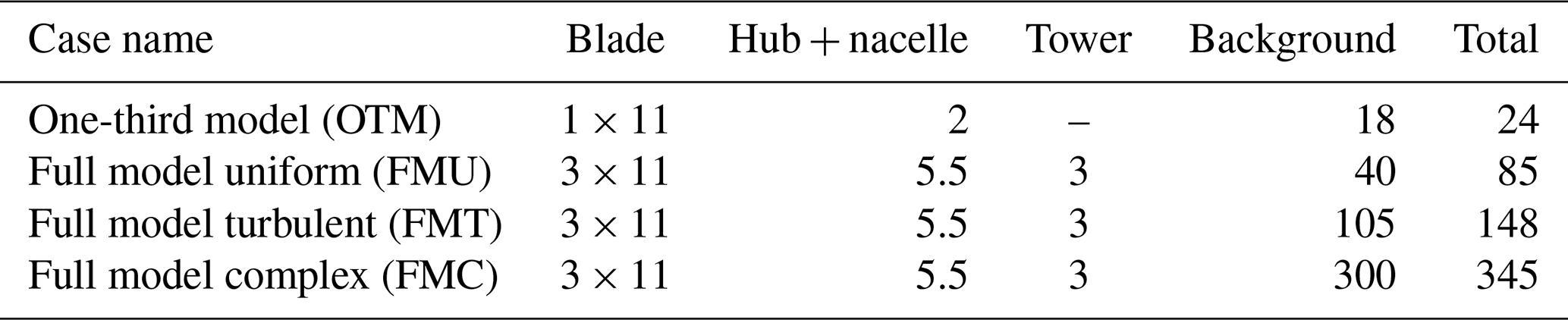
Table 1 gives a breakdown of the mesh sizes in the number of cells for the different setups (that consequently influence the costs of the calculations). The different boundary conditions and CFD models are depicted in Fig. 2. Additionally in Table 2 the dimensions of the different backgrounds are shown in terms of distances from the tower bottom. The complex-terrain mesh is clearly much wider than it is long, and this is done to avoid any influence of the interaction between the periodic boundary condition and the topography, as explained in Letzgus et al. (2021). The mesh discretization occurs via hanging grid nodes, ensuring a resolution of 0.25 m in the closest area to the turbine and increasing up to 2 m for a large area of the domain to ensure a sufficient physical resolution. In the following the meaning of the boundary conditions is clarified:

Table 1 Mesh sizes in millions.

• Navier–Stokes wall represents the ground and surface boundary conditions considering friction.

• Euler wall represents the ground boundary conditions with no friction.

• Farfield denotes where either a fixed velocity or zero extrapolation conditions can be set for the background border.

• Periodic and periodic rot are the symmetrical boundary conditions in the axial and rotational direction, respectively.

• Gust is the FLOWer boundary condition to use when a wind profile and turbulent fluctuations from experiments (or synthetic turbulence) have to be injected in the flow.

The flat terrain for FMU and FMT is different because in FMU no wind profile and no inflow turbulence are considered, and therefore it is possible to use a smaller background and increase the cell size, saving in this way computational time. Table 3 summarizes the operating conditions at which the simulations are run with the corresponding rpm and pitch angles of the turbine. No controller is considered in the simulations; i.e., both rpm and pitch angle are kept constant. OTM and FMU represent the rated conditions of the blade, while FMT and FMC are based on sheared turbulent inflow conditions extracted from real wind measurements on 31 March 2019 at 23:00 local time (Berlin).

The chosen time step is the same for all coupled simulations and is related to 1 azimuthal degree. This has been chosen to be stricter than for the only stiff simulation, which, for example, in the complex-terrain case was set to 2 azimuthal degrees. On the other hand, Sayed et al. (2016) showed that for the previous version of their coupling used, a 1-azimuthal-degree time step is necessary. The number of sub-iterations needs to be adapted according the coupling type, and this will be addressed in the following sections. The turbulence is injected in terms of fluctuations that are superimposed onto a sheared uniform inflow. The fluctuations have been extracted from experimental time series at the WINSENT test field from already-installed met masts. The spectra and standard deviations of all velocity components of the different measurement positions were extracted, and synthetic turbulence was then generated with the Mann model. The main focus was to match the measured turbulence as well as possible, especially at the hub height. It was then important to make the cases with flat and with complex terrain as consistent as possible. That is why, while the turbulence fluctuations were kept the same, the wind shear coefficient and the mean velocity had to be accordingly changed to keep the same shear and hub height velocity after the slope for both cases at the turbine position. This is necessary because the hill of the complex terrain has an acceleration effect on the flow, and therefore a lower reference velocity has to be taken into account upstream of the hill in order to obtain the same mean hub velocity between flat and complex terrain. In the observed time period the atmosphere was neutrally stratified. More information on how the turbulence is injected inside the computational domain is given in Letzgus et al. (2021). The CFD model of the complex terrain is depicted in Fig. 3, where the presence of the forest can also be noticed. The forest is modeled as additional grid structures by the use of the chimera technique in which force terms are added depending on the foliage density and tree height, as described in Letzgus et al. (2020). In this way the modeling can be very easily adjusted to the seasonal conditions and the form of the forest.

Table 2 Background dimensions in rotor diameters from the tower bottom. Values are approximated and referred to the tower center.

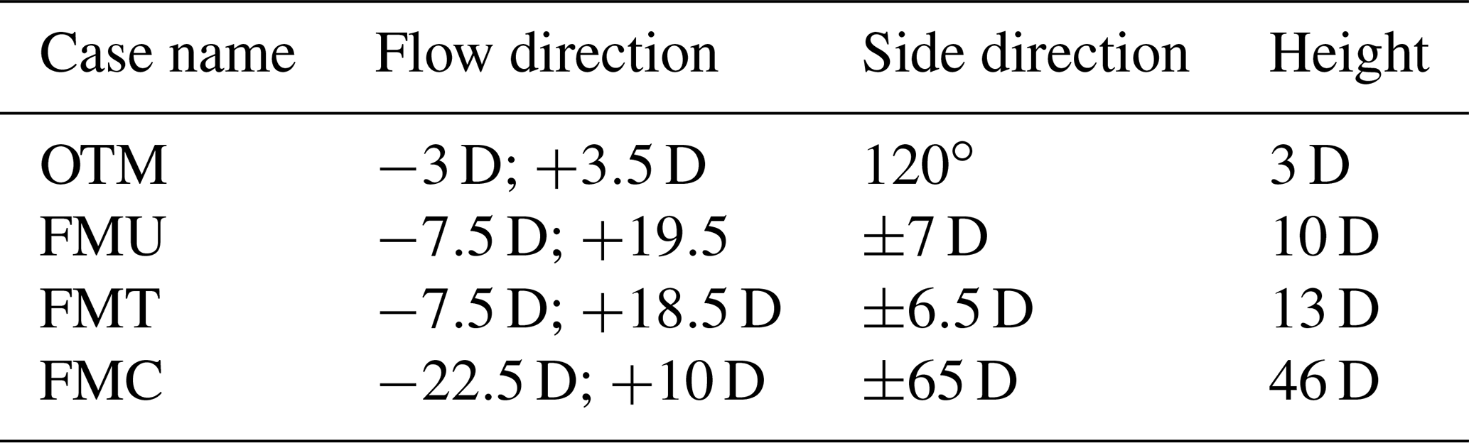
Table 3 Setup of the computed cases (effective conditions at the turbine position).

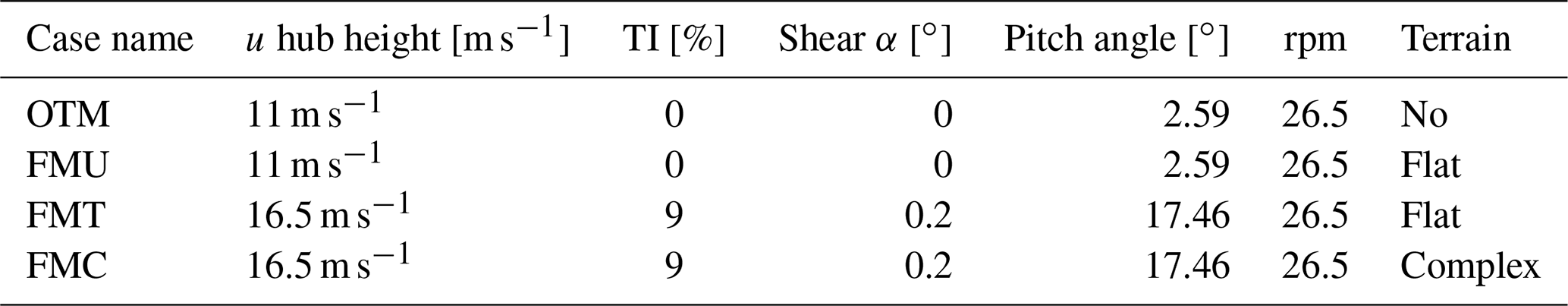
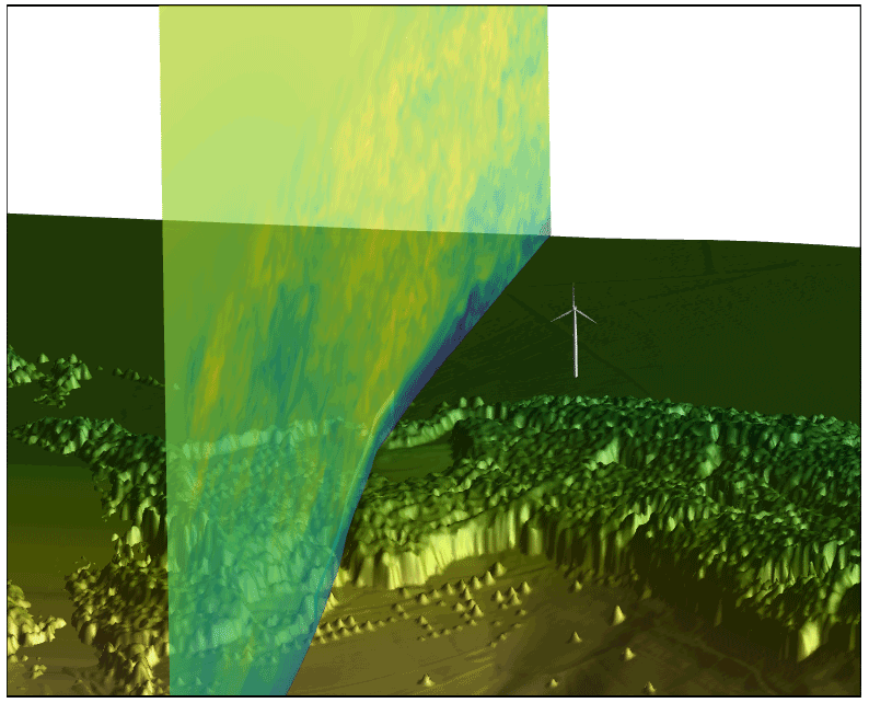
Figure 3 CFD model of the complex terrain considering the forest with a slice of the velocity field 2.5 D from the turbine on its right-hand side.

2.1.2 CSD models

The CSD code applied within this study is the solver Kratos Multiphysics (Dadvand et al., 2010). Kratos was utilized to both generate the structural models and calculate the structural response. Additionally, it served as coupling interface between the solvers.

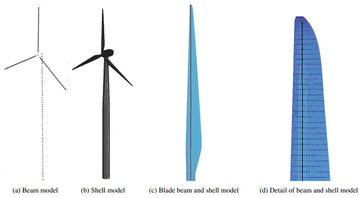
Two structural models have been created for the turbine, one with beam elements and one with shell elements, respectively. Both models take into account geometric nonlinearities, and nonlinear dynamic analysis is applied to solve the turbine structural model. The main physical differences between both models are that in a beam model the cross-section aerodynamic shape deformation is neglected. Secondly, the beam theory implemented in Kratos does not consider bend–twist coupling, while the shell theory contemplates it intrinsically. Rayleigh damping is used to model the damping properties of the turbine, adapting the coefficients to each coupled structure.

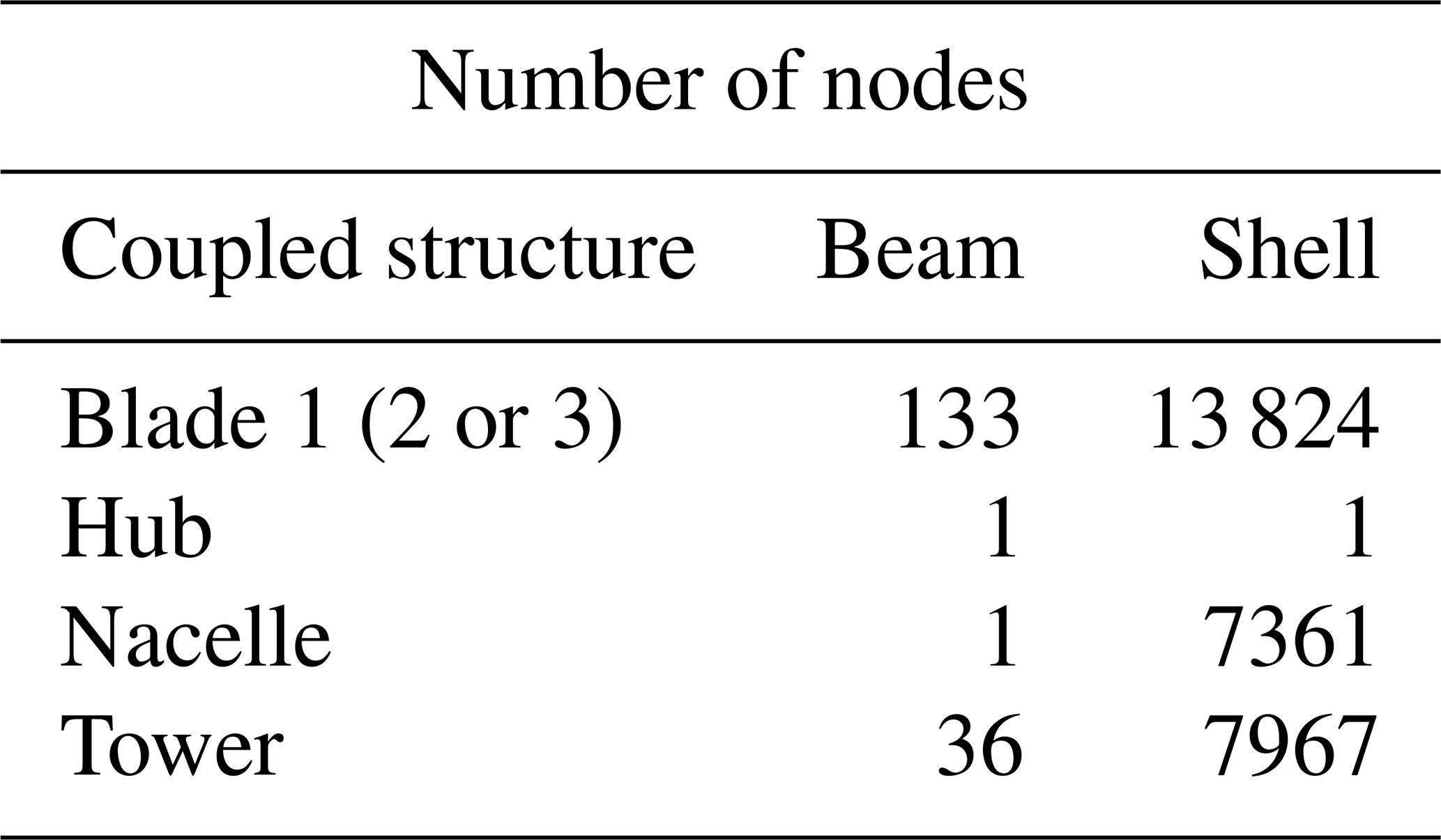
From a practical point of a view, a beam model and a shell model strongly differ in terms of the number of computational nodes, as shown in Table 4, in which it can be noticed that the hub has been modeled in both cases as a single point. This influences directly the computational time. Both structural models are depicted in Fig. 4c.

Table 4 Number of nodes/elements for each structure in both beam and shell models.

Figure 4 Beam and shell structural models.

The shell coupling needs a mapper to interpolate the loads between the CFD and CSD meshes. In this study the Mortar mapper (Wang, 2016) is chosen in Kratos, as it was before in Sayed et al. (2016). This is not necessary to map the deformations because these are directly communicated to FLOWer, which uses them as a cloud of points around the structures, deforming them according to a radial-basis-function (RBF) algorithm.

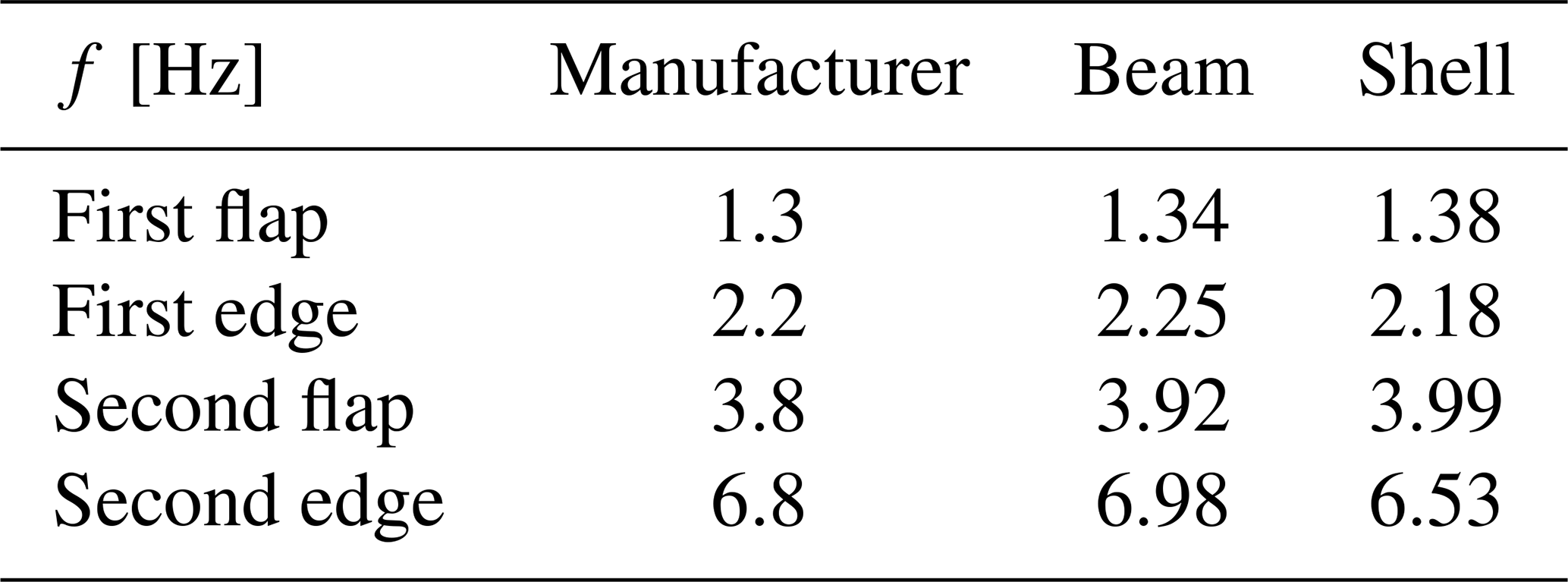
In Kratos it is possible to evaluate the eigenfrequencies of the structural model. The manufacturer delivered the first four eigenfrequencies of the blade, which are compared in Table 5 to the beam and shell models, respectively.

Table 5 Comparison of the first four eigenfrequencies of the blade.

The entire turbine is modeled in both beam and shell models, in which it is clear from Table 4 that the rotor represents around 90 % and 80 % of the total number of cells for the beam and shell, respectively. For more information about the structural models used within this study, please refer to Sayed et al. (2020) and Bucher (unpublished).

2.1.3 FSI coupling and performances

The FLOWer–Kratos coupling has been developed within the WINSENT project in cooperation with the Lehrstuhl für Statik of TUM. It is based upon the coupling employed by Sayed et al. (2016) within FLOWer and Carat$++$. It consists of a partitioned approach with both explicit and implicit algorithms; i.e., the communication between the two solvers happens once (explicit) or several times (implicit) per physical time step. Both nonlinear beam and shell elements can be coupled, and both rotating and non-rotating components can be taken into account, allowing us to consider the aeroelasticity of the complete turbine. The communication bases on FileIO and the logic tree are depicted in Fig. 5. The two solvers start independently, and a mesh initialization check takes place at the beginning to ensure a correct mapping of forces and deformations between the CFD and CSD meshes. Kratos is the first solver, sending either zero deformations (at the very first coupling time step) or the last-saved deformations. FLOWer deforms the surface and the surrounding meshes according to a radial-basis-function (RBF) algorithm. A direct application of the deformation occurs during the shell coupling because the deformations are mapped by Kratos directly on the real CFD surface grid. Afterwards, the time step calculation as prescribed in Sect. 2.1.1 takes place and the resulting aerodynamic forces are calculated. These are either the forces on the three directions in space over all surface cells (in the case of shell coupling) or three forces and three moments integrated according to the communication nodes (in the case of beam coupling). Kratos receives the input from FLOWer, maps it on the structural mesh, and adds the centrifugal and gravitational forces. The structural time step is then performed, and the resulting deformations are calculated. In the case of an explicit coupling, a new physical time step starts. If the chosen algorithm is implicit, the time step is repeated until reaching a predefined convergence criterion of the deformations.

Figure 5 Logic tree of the FSI coupling.

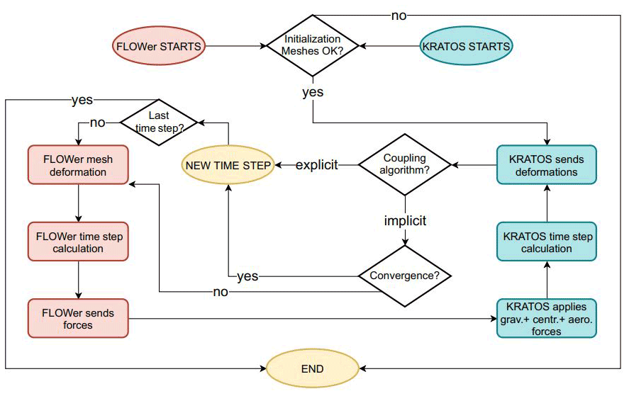
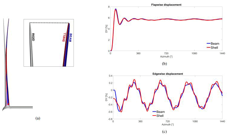
Figure 6 One-third model (OTM), rigid and deformed blade beam vs. shell. Deformations are normalized according to the blade radius and shown as a percentage of it.

One of the main differences between a beam and a shell coupling is the number of degrees of freedom (DOFs) necessary to fully describe the total deformation. A beam element needs 6 DOFs (three translations and three rotations) that are calculated in Kratos on prescribed nodes at the shear centers. On the other hand, a shell only requires three translations because the entire outer shape of the turbine is taken into account. The choice of the shear centers as communication nodes in the beam coupling is not random because a beam model in Kratos does not consider bend–twist coupling. The shear center is by definition the point on which a shear force causes no twist, and a torque moment causes no displacement of the shear center, as also described in Fedorov (2012). A shell model, on the other hand, considers intrinsically a bend–twist coupling. As shown in the structural model description in Sect. 2.1.2, a shell model has many more nodes than a beam model, and therefore its computational time is not negligible anymore as in the case of a beam model. All calculations have been run on the SuperMUC-NG supercomputer at the Leibniz-Rechenzentrum in Munich, and an example of the computational time for each configuration is given in Table 6. As it can be seen, FSI computations based on a beam model of the blade/turbine increase the computational time by around 50 %. The CSD calculation time is negligible in this case, and almost the entire computational time is driven by the CFD part. The increase in computational time is because the number of inner iterations per time step has to increase in order to reach the same convergence level as only CFD. Shell-based FSI calculations additionally have a longer computational time for the CSD solver due to the high number of structural elements, which results in CFD representing only ∼75 % of the average time step. The computational time of the case “full turbine” is considered for uniform inflow conditions, which is the cheapest case from the CFD side.

Table 6 Performance of the FSI coupling based on beam and shell elements in comparison to pure CFD calculations, in CPU per hour per time step (1 azimuthal degree) on average over one revolution.

All coupled simulations that will be analyzed in the following sections started from already-run stiff cases in order to accelerate the convergence in flexible conditions and reduce the transition times.

3 Results

3.1 One-third model (OTM) with laminar uniform inflow

An OTM calculation of a wind turbine is a highly efficient way to obtain a first insight into the turbine performances and, in the case of the development of a new FSI coupling, to test its functioning, capabilities and limitations. The rigid simulation of the OTM case has been firstly run for more than 20 revolutions to ensure the loads' convergence and the correct wake development. Afterwards, 5 revolutions have been computed with flexibility using a time step equivalent to 1 azimuthal degree with an explicit algorithm, reaching the complete convergence of the deformations. As described in Sect. 2.1.2, the two structural models are consistent within each other, and the tip deflection differs by less than 1 %. Linear models lead to a nonphysical elongation of the blade when bending. This drives to large errors in the deformation evaluation, especially when long blades are taken into account. In fact the elongation generates a larger surface of the blade with consequently higher loads and therefore larger bending deformations. This does not happen with the nonlinear models applied in this study, as can be seen in Fig. 6a.

Figure 7 Blade sections enlarged in the y direction and c_l calculations for $r/R=\mathrm{50}$ % and $r/R=\mathrm{95}$ %.

The tip deformations in flapwise and edgewise directions are depicted in Fig. 6b and c. The normalized root mean square deviation (NRMSD) is around 1 % and therefore negligible. Because the damping is implemented in exactly the same way in both models, this difference is to be associated with only the structural model. The sectional torsion has been calculated from the surface output files because the shell coupling communicates only the displacements in the three directions. A reference section at the tip of the rigid blade has been taken into consideration, and its indexes have been used to find the same section on the deformed blades. The deformed sections have been afterwards unrotated using Rodrigues' rotation formula to make them parallel to the rigid section. Aligning then the leading edges, it is possible to evaluate the torsion angle at the section. The average value of the torsion in the case of beam coupling is 0.1138^∘, while for the shell model it is 0.138^∘. The blade is very small, and that is why the torsion is negligible. The small difference between the beam and shell is to be reconnected to the neglecting of bend–twist coupling in the beam model.

An added value of a shell model is that airfoil deformation can be predicted. Although this can be very limited, noticeable changes in the camber can have an impact in terms of lift and drag coefficients of the airfoil (i.e., the polars). That is why two sections of the deformed and undeformed blade have been extracted, opportunely rotated to make them parallel within each other and analyzed with XFOIL (Drela, 1989) afterwards. Viscous polar calculations have been performed fixing $Re=\mathrm{4}\times {\mathrm{10}}^{\mathrm{6}}$ and Mach =0.19. The results are depicted in Fig. 7, and no difference could be detected in the outer region, while a light cambering in the middle blade region appeared, leading anyhow to only around a 1 % difference in the lift coefficient. It can be therefore concluded that for the applied inflow conditions (that are also the standard operating conditions), the usage of only a beam model for this turbine in comparison to a shell model leads to a negligible difference that does not justify the higher computational cost.

3.2 Impact of the structural model and coupling algorithm

In this section the use of beam and shell elements is compared for the turbulent inflow case in complex terrain (FMC) in Fig. 8. This has been chosen because it represents the most complex case from the aerodynamic point of view and therefore is of interest to studies about the structural impact. In these cases the entire turbine is considered flexible.

Figure 8 Flapwise (a) and edgewise (c) blade tip deformation over three revolutions, with comparison of beam and shell coupling. Panels (b) and (d) show the FFT over a 1 min simulation. A 1D moving-average filter has been applied for clearness. Dotted vertical lines are plotted at the first flapwise and edgewise eigenfrequency of the blade, respectively.

The choice of the structural elements shows on average a difference of 3.7 % of the root mean square (rms) value of the shell flapwise deformation, which is not negligible anymore in comparison to the OTM case. The difference becomes much stronger in the edgewise direction, where an average difference of 15 % of the rms value occurs. The higher-frequency oscillations are more strongly pronounced in the shell coupling, which can be traced back to the absence of coupling terms in the stiffness matrix of the beam model (bend–bend and bend–twist). On the other hand a complete modeling of the geometry is done in the shell model, justifying the differences that are occurring.

The FFT of the signals over 1 min is depicted in Fig. 8b and d. It can be seen that the first harmonic of the rotational velocity (commonly known as 1P) shows clearly the strongest peak in the case of the edgewise deformation, suggesting the importance of the weight effect for this deformation direction. On the other hand, the 1P frequency does not clearly deviate from the neighboring peaks in the flapwise direction, while the strongest peaks are only at higher frequencies. This shows that, in this case, the low-frequency spectrum of the flapwise deformation is mostly influenced by the turbulent inflow and not the blade–tower passage. The spectrum amplitude in the case of the shell coupling is always slightly higher than in beam coupling (especially in edgewise) although the rpm harmonics' amplitudes are always close to each other. This has been attributed again to the absence of some coupling terms in the stiffness matrix of the beam model and the higher accuracy of the shell model in which the entire geometry is taken into account. Only the rpm harmonic close to the edgewise eigenfrequency of the blade shows a higher amplitude in shell than in beam coupling. This suggests that in the case of particular excitation of the edgewise eigenfrequency, an aeroelastic instability could take place that the beam coupling would not recognize.

The improvement in accuracy by using an implicit coupling is now discussed. In this case the computational time increases due to the repetition of the time step. The implicit coupling has only been considered for the FMC case with shell coupling. A total of three revolutions with a time step equivalent to 1 azimuthal degree have been computed. In order to reach the predefined convergence, it was necessary to perform more coupling iterations per time step about 28 times per revolution. An FFT of the flapwise and edgewise tip deformation is depicted in Fig. 9. Almost no difference can be seen between the two algorithms in this application, and that is why all following investigations have been based on only an explicit algorithm.

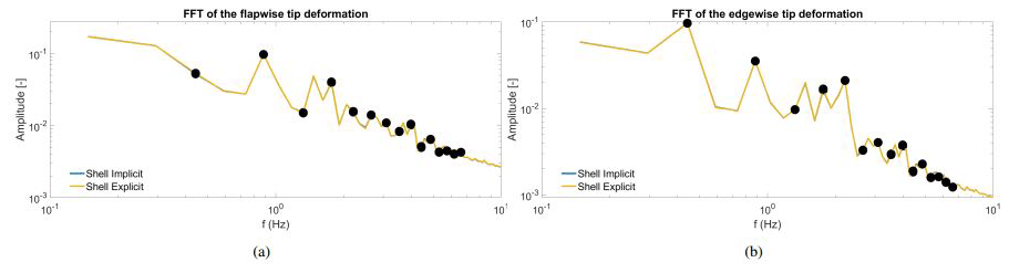
Figure 9 FFT of the flapwise and edgewise blade tip deformation using shell elements with an explicit and implicit coupling algorithm. Circle on the rpm harmonics.

3.3 Aeroelastic effects on the near wake

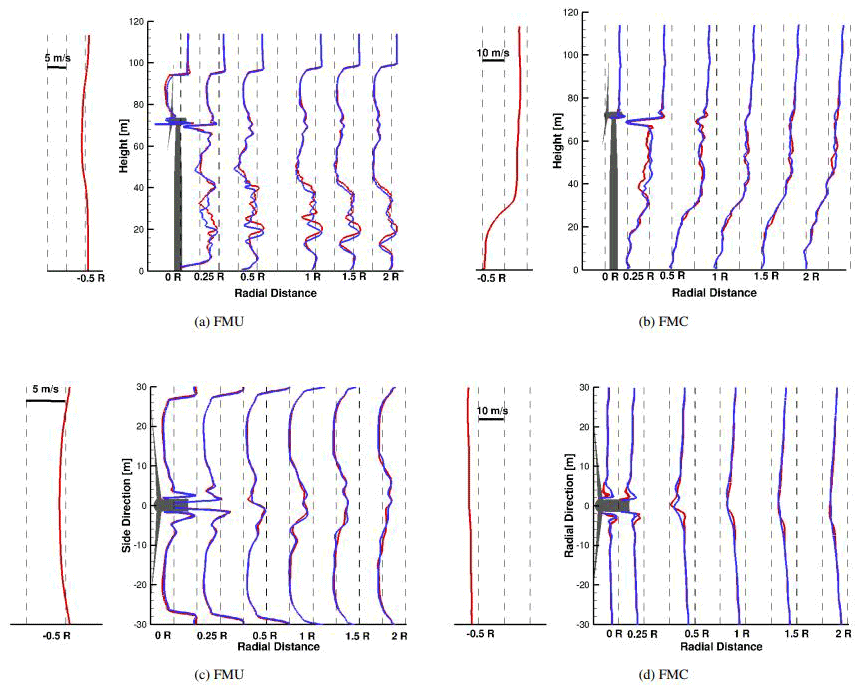
Figure 10 Profiles of the velocity component in the wind direction at different axial distances from the tower center. x–z (flow direction–height) slices in (a) and (b) and x–y (flow–side direction) slices in (c) and (d), including the averaged inflow slice. Red lines represent the rigid case and blue lines the beam-coupled case.

In this section the effects of flexibility on the near wake are analyzed. For this reason wind velocity profiles have been extracted at defined radial distances from the hub center and averaged over three revolutions. The rigid and coupled simulations have been run in parallel so that the same time series could be taken into consideration and averaged. The wind profiles have been extracted for two sections, an x–z (flow direction–height) plane through the tower axis and an x–y (flow and side direction) plane through the nacelle axis. The cases taken into consideration are FMU and FMC, comparing in both cases the rigid (red lines in Fig. 10) with the beam-based FSI simulation (blue lines). The first has been chosen because it is the uniform inflow case and therefore the simplest one and the second one because it is closest to reality. Because of the higher inflow velocity and the higher pitch in the FMC case, the induction of the rotor decreases. This can be seen in Fig. 10b, where the influence of the rotor presence on the wake shape is negligible. For both FMU and FMC the upper part of the rotor is shown to be less influenced by flexibility, where only a small shape discrepancy can be noticed in the section closest to the rotor. On the other hand, the lower part of the rotor wake mixes with the tower wake, showing different profile shapes up to a distance of 2 R in the area between 15 and 50 m height. The tower is very stiff, and especially in this region its deformation is negligible in comparison to the blade and cannot therefore change the wake shape. This suggests that the discrepancy has to be traced back to the blade–tower interaction. In FMU, where the velocity is kept constant, the blade–tower interaction has a strong impact, and that is why wake profile differences can be seen at up to 2 R distances. This effect is lower in Fig. 10b because the rpm harmonic peaks of the flapwise blade deformation are not much stronger than the turbulence peaks as seen in Sect. 3.2.

Figure 11 Vertical plane with interaction of the turbulent inflow in flat terrain (a) and complex terrain with forest (b). Average TI over 1 min in a plane 1 R upstream rotor position (c).

On the other hand, the y–z sections in Fig. 10a and b are extracted at the hub height and are therefore not influenced by the tower wake. As in the upper part of the rotor in x–z planes, no influence of the wake shape can be noticed independently of the blade pitch angle. Due to the oscillating movement of the nacelle, the hub region shows small discrepancies that already disappear after 2 R radial distances.

3.4 Difference between flat and complex terrain including flexibility

Both FMT and FMC consider the same turbulent inflow field as input at the inlet, propagating on a flat terrain and up a hill with a forest, respectively. This also means that the time needed by the flow to reach the turbine is not the same between the two cases, and therefore differences between flat and complex terrain can only be extrapolated from long simulations in a statistical way. Simulations of 1 min have been computed for all cases, as a compromise between computational time and statistical requirements. On the other hand, when the effects of aeroelasticity are of interest, it is possible to compare rigid and coupled simulations time step by time step as long as the real time series chosen coincide. Figure 11b shows the influence of the forest, leading to very low velocities especially for 40 % of the tower. Here a strong cut between a low-velocity and a high-velocity region occurs, which is completely absent in the case of the flat terrain, which only has shear effects (in addition to turbulence). Additionally, structures of the forest with low velocity and high TI reach the lower half of the rotor as shown in Fig. 11c, with direct consequences on loads and deformations.

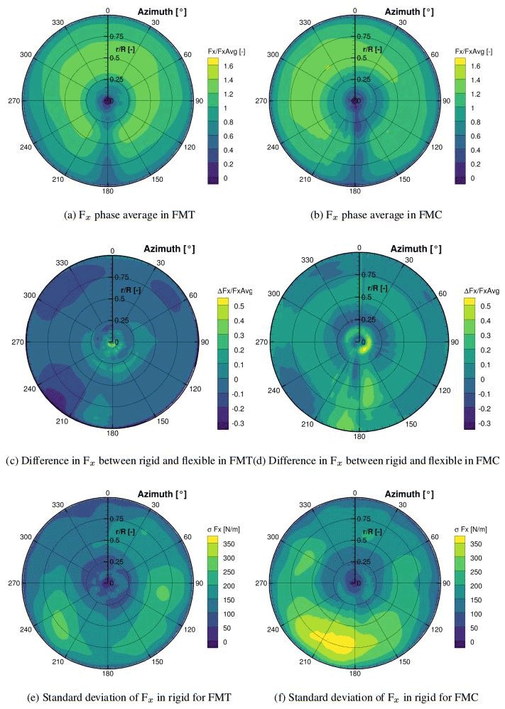
Figure 12 Phase average of the thrust force of one blade calculated over 26 revolutions. Loads are normalized according to the average in FMT and FMC, respectively. Difference is calculated as (F_x flexible)−(F_x rigid). Standard deviation is calculated for the rigid case.

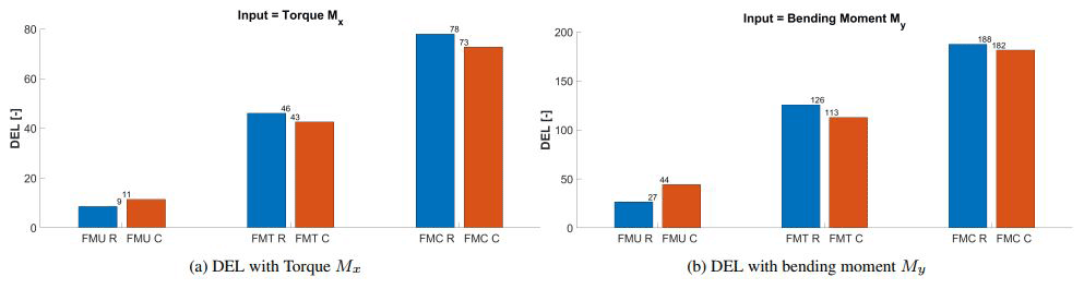
Figure 13 Normalized DEL calculation comparison between rigid (blue) and coupled (red) for the cases FMU, FMT and FMC.

The effect of the blade deformation on the blade loads is then analyzed for both FMT and FMC. As described in Sect. 2.1.1, those two cases use turbulence with a different shear coefficient and u_∞ to ensure the same hub velocity close to the rotor. The phase-averaged thrust force (F_x) calculated over 26 revolutions (about 1 real minute) for the rigid cases is shown in Fig. 12a and b. Figure 12c and d show the respective difference in the case of shell-coupled FSI simulations. Loads are normalized according to the respective average value in the rigid case. It can be seen that in flat terrain the load distribution is mostly symmetric, with lower loads during the tower passage. The tower passage effect can also be seen in the FMC case, although the load distribution between the upper and lower side of the rotor is not symmetric anymore. This is explained by the retreating blade effect (Letzgus et al., 2021) by which the blade faces an inclined flow due to escarpment of the orography. This is in phase with the blade movement on the left-hand side (LHS) of the rotor and opposite to the phase in the right-hand side (RHS) of the rotor. This effects leads to a higher AOA on the left-hand side of the plot than on the right-hand side. This phenomenon also influences the tower region, which is not symmetrical around the 180^∘ area anymore. When both cases are considered flexible, in the flat terrain the largest differences occur at the lower rotor half close to the hub and after the blade–tower passage. Directly after the tower region, i.e., between 180 and 230^∘, the effect of the blade–tower interaction can be depicted. Due to the inertia of the blade, the deformation's peak occurs between 20^∘ after the effective blade–tower passage. Between 180 and 200^∘ the blade faces lower deformation and moves therefore fast against the wind direction. The deformation velocity of the blade tip reaches up to ±3.5 m s⁻¹, which represents around 20 % of the reference velocity at the hub, with a consequent effect on the relative velocity faced by the blade and therefore loads. The opposite happens in the area between 210 and 240^∘, where the blade tip displacement increases again and moves therefore in the wind direction with a lower relative velocity. The same effect can be observed for the FMC case too (Fig. 12d), with a further uniform increase in the thrust in the region between 50 % and 75 % of the blade radius. Additionally from 160^∘ it can be seen that the flexible case develops higher loads. Any connection of this phenomenon with the blade tip deformation due to the blade–tower interaction can be excluded because it occurs at least 40^∘ later. The standard deviation of the thrust for the rigid case is shown in Fig. 12e and f. Here it can be noticed that in the flat case the lower rotor half shows a higher standard deviation, which is due to the presence of shear, while on the other hand the case with the complex terrain shows much higher values in the area between 140 and 250^∘. As shown in Fig. 11c, vortex structures from the forest have a strong influence on the lower rotor half, leading to local low velocities with high turbulence intensities. Summing the retreating blade effect and the forest impact leads to an asymmetrical tower shadow in the rigid case (Fig. 12b). On the other hand, when the blade is bending, the tower shadow impact is more pronounced, becoming again the dominant factor and making the area by 180^∘ more symmetrical again. Additionally, it needs to be considered that the blade presents a cone angle, and therefore bending deformation increases the rotor disk area, counterbalancing the lower velocities due to the forest wake.

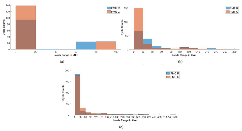
Figure 14 Cycle count using the bending moment M_y for the cases FMU, FMT and FMC, both rigid and shell-based coupled.

3.5 Aeroelastic effects on the damage equivalent loading (DEL)

The DEL is a constant load value that, applied over a defined number of cycles, leads to the same damage as a time-varying load. In this way it is possible to compare different load signals and analyze the factors that influence the fatigue on a structure. The approach is based on S–N curves (stress vs. number of cycles) of the material on a log–log scale and a rainflow algorithm that recognizes peaks, valleys and therefore fatigue cycles. The formulation used in this study is the one of Hendriks and Bulder (1995), which has also been applied in Guma et al. (2021) to the DANAERO rotor. Considering the conclusions from Sect. 3.2, shell-based FSI simulations have been used here to generate the DEL input. In order to consistently compare the cycle counts, 26 revolutions (around 1 min real time) have been taken into consideration. Two different input signals have been chosen, the flapwise (M_y) and edgewise (M_x) blade root moment. The first one is also called the “bending moment”, while the second represents the blade torque. Three cases are compared, FMU, FMT and FMC, and the results of the DEL calculations are depicted in Fig. 13. Both signals show similar results, and that is why only the cycle count of the M_y signals has been considered in Fig. 14. The case with uniform inflow is the one that always shows the lowest damage level and is also the only one in which flexibility slightly increases the damage level. Looking at Fig. 14a, it can be seen that flexibility is not only adding small perturbations to the signal (small cycles between 0–10 kN m) but also increasing the amplitude of the large cycles (the ones generated by the blade–tower passage). The two cases with turbulence always show larger DEL values compared to uniform inflow (FMU). This is a consequence of the much larger number of small cycles (oscillations due to turbulence) and to the presence of a few very large cycles (up to 500 kN m). The flexibility slightly reduces the DEL values, acting as a positive effect in a similar way for both FMT and FMC. In FMT, cycles with amplitudes between 60 and 90 kN m are damped, leading to a higher number of smaller cycles. Similarly in FMC, very few large cycles up to 420 kN m are damped to cause smaller cycles. That is why the DEL value slightly decreases, considering that the brighter the cycle, the larger its influence on the DEL value. It can be concluded that, in the case of turbulence where large cycles are detected, flexibility acts as a damper, reducing them to a higher number of smaller cycles and therefore smaller fatigue values.

Lastly, a comparison of the DEL for the same FMC case has been performed to confront the beam and shell coupling in Fig. 15. For both inputs, the DEL using the shell model is slightly higher because of a larger number of smaller cycles, which fits with the oscillations in the deformations shown in Sect. 3.2.

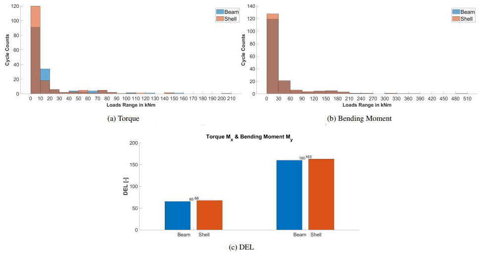
Figure 15 Cycle count using the torque (a) and bending moment (b) and resulting DEL (c). Comparison of beam and shell model by FMC.

4 Conclusions

In the present work, a high-fidelity fluid–structure interaction coupling between the CFD solver FLOWer and the CSD solver Kratos has been presented. The particular features introduced in this coupling are the possibility of using both beam and shell nonlinear structural elements for the entire turbine and of using both an explicit and an implicit coupling algorithm. This coupling has been used to calculate the aeroelastic response and effects of complex terrain on a small-sized wind turbine with around a 50 m rotor diameter and around 750 kW rated power. This turbine is going to be erected in Stöttener Berg in 2022, a complex terrain with the presence of a hill and a forest. The turbine has been therefore simulated by the use of models, increasing their complexity and computational costs from both the aerodynamic–structural and the coupling algorithm point of view. A one-third model of the turbine has been utilized to assess the consistency of both structural models, which shows less than 1 % difference in the case of uniform inflow conditions. The usage of nonlinear models avoided the nonphysical elongation of the blade typical of linear models. A shell model intrinsically considers bend–twist coupling, which is why differences in the predicted torsion occur between the two models, although this is negligible for such a small blade. The section's shape deformation also leads to negligible differences in the lift calculation, and therefore it has been concluded that in the case of single-blade calculations in uniform inflow conditions, a beam-based coupling is sufficient for such a small turbine. When the aerodynamic complexity increases, i.e., when the full turbine in complex terrain is considered, stronger differences occur by adopting either beam or shell structural elements, suggesting that more complicated cases require higher fidelity. Especially in the case that a complex flow combines with aeroelastic instabilities, the usage of only a beam model, which neglects possible occurring vibrations and the section deformation, can result in misleading results. On the other hand it is clear that for only a rough estimate of the loads, the shell model (especially for the entire turbine) is still too expensive from the computational (and pre-processing) point of view. On the other hand, the usage of an implicit coupling shows no advantage at all in comparison to a much cheaper explicit one. Afterwards, the effects on the near wake by means of velocity profiles' shapes have been analyzed for both the uniform inflow case (with a low blade pitch angle) and the case with complex terrain. Cuts at the hub height show that only the hub region is affected by flexibility in both cases. On the other hand, x–z cuts at the tower center show that flexibility only affects the velocity profile region behind the tower due to blade–tower interaction blade deformation peaks. These are more evident in the case of uniform inflow, while they are hidden by the turbulence frequencies in the complex-terrain case and therefore less evident. Then, the impact of the terrain on aeroelasticity has been discussed by means of phase-averaged thrust over a 1 min simulation. The same time series have been computed for both the rigid and the flexible turbine. The blade–tower passage shows here its effect changing the relative velocity between the blade and flow and therefore AOA. The flat terrain was shown to be mostly affected by the shear, while on the other hand, the complex terrain is influenced by low-velocity vortex structures generated by the forest. In this case flexibility already showed its impact directly before the tower passage, with an increase in the loads counterbalancing the lower velocities due to the forest wake.

Finally the effects of aeroelasticity and turbulence are analyzed by means of fatigue calculations (damage equivalent loading). In the uniform inflow case, flexibility leads to a higher number of small oscillations, increases the amplitude of the big cycles and therefore yields a higher DEL. On the other hand, the cases with turbulence show the opposite effect. This is because in the case of turbulent inflow, large cycles are detected and flexibility acts as a damper, breaking them into smaller cycles and therefore smaller fatigue values.

The possibility of making such high-fidelity calculations in feasible time opens new horizons to further topics such as aeroelastic instabilities, e.g., local buckling analysis and vortex-induced vibrations (VIVs), for which BEM-beam models still struggle to provide information. The next steps of this work will be the validation of the obtained results with the field data that will be produced after the building of the two research wind turbines in Stöttener Berg. Additionally it is foreseen that a controller will be introduced, which might have a strong influence on the results especially at high velocities. The way for reliable load prediction for design purposes is still challenging, but it is important to take one step at a time. It is the authors' hope that this work represents one of those steps.