Lidar-assisted model predictive control of wind turbine fatigue via online rainflow counting considering stress history

The formulation of parametric online rainflow counting implements the standard fatigue estimation process and a stress history in the cost function of a model predictive controller. The formulation is tested in realistic simulation scenarios in which the states are estimated by a moving horizon estimator and the wind is predicted by a lidar simulator. The tuning procedure for the controller toolchain is carefully explained. In comparison to a conventional model predictive controller (MPC) in a turbulent wind setting, the novel formulation is especially superior with low lidar quality, benefits more from the availability of wind prediction, and exhibits a more robust performance with shorter prediction horizons. A simulation excerpt with the novel formulation provides deeper insight into the update of the stress history and the fatigue cost parameters. Finally, in a deterministic gust setting, both the conventional and the novel MPC – despite their completely different fatigue costs – exhibit similar pitch behavior and tower oscillations.

1 Introduction

Fatigue is damage of a material caused by cyclic application of mechanical stress. For wind turbines, fatigue has a large impact on lifetime, for example, of tower, blades, and drivetrain and is a main design driver. Model predictive controllers (MPCs) enable optimal control of turbines by utilizing predictions of the incoming wind by a light detection and ranging (lidar) device (Bottasso et al., 2014; Schlipf et al., 2013). Based on these input predictions, stress time series at crucial spots in the turbine structure can be predicted. Rainflow counting (RFC) is the standard method for the decomposition of stress time series for fatigue estimation. Until recently, RFC could not be implemented in MPCs (Barradas-Berglind and Wisniewski, 2016) and could only be used for post-processing of measured and simulated data. In Loew et al. (2020a), an MPC formulation was presented that externalizes the RFC evaluation and includes its results back into the MPC via time-varying parameters. Therefore, this formulation is referred to as “parametric online rainflow counting” (PORFC). PORFC allows for the direct and rigorous incorporation of fatigue in the cost function or constraints of MPCs.

In PORFC, fatigue is calculated based on stress information from the prediction horizon of the MPC, which is in the order of a few seconds. However, fatigue is a long-term effect in which stress cycles are usually defined on much longer time spans. Therefore, in Loew et al. (2020b) PORFC was combined with a systematic incorporation of historic stress samples (“residue”). In the same work, this formulation was simulated in an idealized setting in which only a few degrees of freedom (DOF) in the plant turbine model were activated and in which full information about the incoming wind and the turbine states was assumed.

The main goal of the present work is to thoroughly assess the formulation in a more realistic simulation scenario. Particularly, a mismatch is introduced between the MPC-internal and the plant models, a moving horizon estimator provides initial state estimates for the MPC, and a lidar simulator is utilized to generate a realistically imperfect wind estimate. The assessment is performed in several turbulent as well as deterministic gust scenarios.

This paper is organized as follows. In Sect. 2, the phenomenon of fatigue and cycle identification are reviewed. This analysis is the basis for an application-focused description of PORFC in Sect. 3. In Sect. 4, a moving horizon estimator is formulated. In Sect. 5, the controller toolchain and the tuning of each of its elements are presented. Finally, PORFC is compared to a conventional MPC and to a conventional proportional integral derivative (PID) controller in the above-mentioned simulation scenarios.

2 Review of fatigue estimation

In the following, fatigue is defined, cycle identification is explained, and the concept of residue is presented.

2.1 Definition of fatigue

In the following, the phenomenon of fatigue is defined for conditions and assumptions that apply to the wind energy domain: namely mechanical fatigue, normal ambient temperatures, neglection of irreversible strain effects, and invariance with respect to time. In this setting, fatigue is damage of a material caused by cyclic application of mechanical stress. Without loss of information, the fatigue impact of a given stress-trajectory can be analyzed solely based on its extrema or “reversals”. This implies that the shape and contained frequencies of the original continuous stress trajectory are considered to be irrelevant for fatigue estimation (Barradas-Berglind et al., 2015). Therefore, the fatigue impact of a reversal sequence is fully determined by its contained individual stress cycles. Each stress cycle can be represented by a cosine function. A stress trajectory typically contains full cycles, which are cosines of a full period, and half cycles, which are cosines of only a half period. Half cycles therefore represent either a rising or falling transient. Instead of storing three (full cycle) or two (half cycle) stress samples, it is common to store two stress samples and a weight, which is valued w_c=1 (full cycle) or w_c=0.5 (half cycle). The two stress samples can be the cycle stress maximum and minimum or the stress amplitude σ_a, c and mean σ_m, c. Instead of stress amplitude, stress range ${\mathit{\sigma }}_{\mathrm{r},c}=\mathrm{2}{\mathit{\sigma }}_{\mathrm{a},c}$ is frequently used as well.

Typically, fatigue impact of a stress cycle mainly correlates with its stress amplitude: a positive stress mean increases whereas a negative stress mean decreases fatigue impact. Quantitatively, this mean stress effect is expressed by the Goodman equation (Haibach, 2006) (p. 184), which leads to the equivalent stress σ_eq, c. Consequently, equivalent stress is used to calculate the number of cycles to failure,

$$\begin{array}{}\text{(1)}& N_c=f_{\mathrm{SN}}^{-\mathrm{1}}\left({\mathit{\sigma }}_{\mathrm{eq},c}\right),\end{array}$$

via the inverse S–N or “Woehler” curve, which typically has a piecewise definition over the stress axis. Fatigue damage of a given stress cycle,

$$\begin{array}{}\text{(2)}& D_{\mathrm{fatigue},c}=\mathrm{1}/N_c,\end{array}$$

is obtained by the reciprocal of the number of cycles to failure. Total damage of the given stress trajectory is obtained by linear accumulation $D_{\mathrm{fatigue}}={\sum }_c{D}_{\mathrm{fatigue},c}$ of damages of individual stress cycles according to the Miner–Palmgren rule (Miner, 1945).

2.2 Cycle identification via the rainflow algorithm

Cycle identification is straightforward if, for example, a simple sinusoid is analyzed. There, amplitudes, mean values, and number of cycles are obvious. However, realistic stress trajectories usually are highly complex and contain stress cycles that can be nested (“nested cycles”). Additionally, half and full cycles can be present, as stated above. The most widely accepted algorithm for cycle identification from complex trajectories is the rainflow(-counting) algorithm (RFC) (ASTM International, 1985). A flowchart of the rainflow algorithm is displayed in Fig. 1.

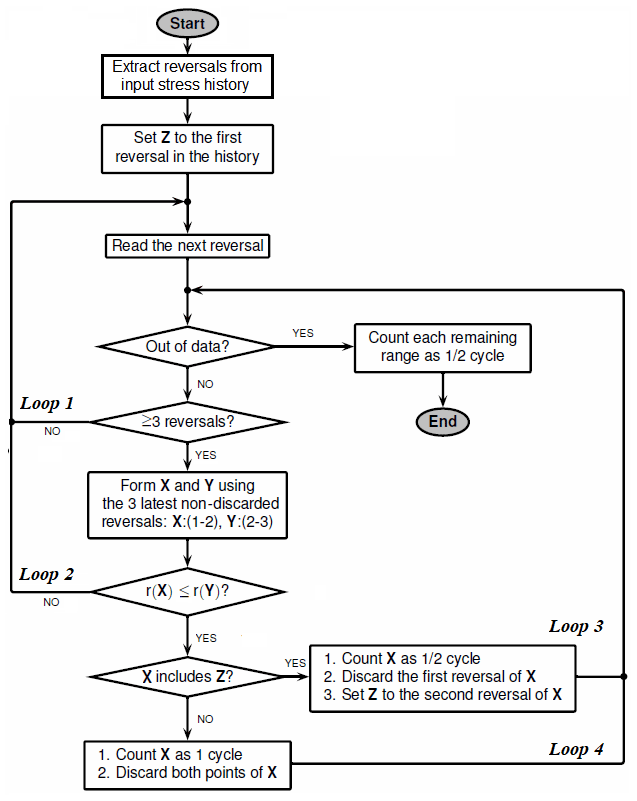
Figure 1 Flowchart of the MATLAB implementation rainflow() of the three-point algorithm (simplified from The MathWorks Inc., 2018). Stress extrema are called “reversals”. The range $r\left(\mathit{X}\right)=\left|X\right(\mathrm{2})-X(\mathrm{1}\left)\right|$ of a stress value pair X is the absolute value of the difference between both stresses.

At the beginning of the algorithm, RFC receives as input a stress trajectory and extracts its reversals (extrema). Throughout the algorithm, reversals are read consecutively from left to right. Each new reversal is stored in an operational memory. From this memory, cycles are identified based on a triplet of reversals. The Rainflow algorithm contains four main loops. Loop 1 initiates the reading of a new reversal sample if fewer than three reversals are in the operational memory. Loop 2 initiates the reading of a new reversal if, based on the current operational memory, no cycle could be identified. Loop 3 and Loop 4 initiate the subsequent check for a cycle in the current operational memory and are triggered after identification of a half or full cycle, respectively. A more comprehensive explanation of the algorithm can be found in The MathWorks Inc. (2018).

As shown above, the Rainflow algorithm contains algorithmic branches and loops. Thus, a crucial property of the Rainflow algorithm is its discontinuous output behavior. Furthermore, the number N_c of identified cycles is not known before execution but bounded by the number of extrema.

The characteristics of the identified cycles that are output by RFC for each cycle c are stress range σ_r, c [Pa], stress mean σ_m, c [Pa], sample index of cycle start k_start, c [–], sample index of cycle end k_end, c [–], and cycle weight w_c [–]. In the present work, these characteristics will be used in a converted form of stress amplitude σ_a, c [Pa], stress mean σ_m, c [Pa], sample index of cycle maximum k_max, c [–], sample index of cycle minimum k_min, c [–], and cycle weight w_c [–].

2.3 Batchwise cycle identification and residue

As shown in Loew et al. (2020b), wind turbine stress trajectories can contain long-term cycles. Thus, the Rainflow analysis has to be carried out over the entire length of an available stress trajectory. For offline purposes, this mode is perfectly adequate. However, for online monitoring and control, a complete Rainflow analysis for each newly measured stress sample is computationally infeasible. As a solution, Heinrich et al. (2019) showed that Rainflow analysis can be performed batchwise if a so-called “residue” is used for carrying along the half-cycle stress samples. Residue, therefore, denotes a set of stress samples that occurred in the past and have not formed full cycles as yet.

Depending on the stress signal, a high number of samples can be accumulated in the residue. The maximum possible length of the residue vector results from diverging and converging stress time series because they generate a large number of half cycles (Köhler et al., 2012). However, long-term diverging series are unrealistic because unstable machine behavior typically is counteracted by the controller or an emergency shutdown. Long-term converging series are irrelevant since very low-amplitude cycles can be discarded without significant errors in fatigue estimation. To conclude, the length of the residue vector is finite and remained well below 100 in practical tests (Loew and Obradovic, 2020).

3 Fatigue in model predictive control of wind turbines

Wind turbine fatigue is usually implemented in MPC within the cost function. Common cost types in MPC are stage cost and terminal cost. Stage costs comprise a summation of state samples or a time integral of state trajectories over the prediction horizon and are preferred for the present application. Terminal costs are defined as a function of the sole state samples at the end of the prediction horizon (Grüne and Pannek, 2017). Alternatively, fatigue can also be used as a constraint, for example, to express a desired lifetime goal.

3.1 Indirect fatigue metrics in MPC

Several approaches reported in the literature involve indirect fatigue metrics (Barradas-Berglind and Wisniewski, 2016; Gros and Schild, 2017; Evans et al., 2015). However, indirect fatigue metrics have two main disadvantages:

• Instead of actual damage, only a damage-related value is obtained and optimized.

• Indirect fatigue terms have different units from harvested energy. Thus, weighting both terms in the cost function is not straightforward.

When considering tower fatigue, the most common approach involves the quadratic penalization of tower tip deflection rate ${\dot{d}}_{\mathrm{T}}$. This also can be interpreted as a penalization of kinetic energy of the lumped tower mass m_T, averaged over the prediction horizon T_horiz. In the present work, therefore, the stage cost,

$$\begin{array}{}\text{(3)}& J_{\mathrm{fatigue},\mathrm{TTVP}}=\underset{t_{\mathrm{0}}}{\overset{t_{\mathrm{end}}}{\int }}{\displaystyle \frac{\mathrm{1}}{\mathrm{2}{T}_{\mathrm{horiz}}{P}_{\mathrm{g},\max }}}{m}_{\mathrm{T}}{\dot{d}}_{\mathrm{T}}^{\mathrm{2}}\mathrm{d}t,\end{array}$$

is used for comparison and referred to as “tower tip velocity penalization” (TTVP). An additional division by rated power P_g, max is used for scaling the cost, which is beneficial for optimization.

3.2 Direct fatigue metrics in MPC

In contrast to indirect fatigue metrics, direct fatigue metrics return actual damage. As shown in Sect. 2, direct fatigue estimation involves the Rainflow algorithm. Implementation of RFC within a gradient-based optimization seemed impossible until now due to the following obstacles:

• RFC is a function of all stress samples. Therefore, the concept of neither stage nor terminal cost applies.

• RFC contains branches. Therefore, it exhibits discontinuous outputs and is not continuously differentiable.

• RFC contains “while” loops, which lead to a changing function execution structure depending on the stress input.

Thus, in all known references, the Rainflow algorithm is approximated to some extent. In Sanchez et al. (2015), a version of simple range counting is applied, which is standardized in ASTM International (1985). In Barradas-Berglind et al. (2015), hysteresis operators are used to adapt parameters of a cost function in MPC. This cost function penalizes deflection rates, comparable to TTVP. In Luna et al. (2020), damage estimation including standard RFC is performed on a large number of stress time series, which are used to train a surrogate artificial neural network (ANN). The latter seems to be very promising in terms of correct damage estimation. However, the approach involves a high a priori effort in setting up the ANN, as well as a significantly increased computational load in the MPC (Luna et al., 2020).

Stress history is not included in any of these approaches. In Barradas-Berglind et al. (2015), the hysteresis operators only have memory of damage evolution. Similarly, in Luna et al. (2020), only the previous fatigue rate output of the ANN is memorized until the next evaluation.

3.3 Parametric online rainflow counting - concept

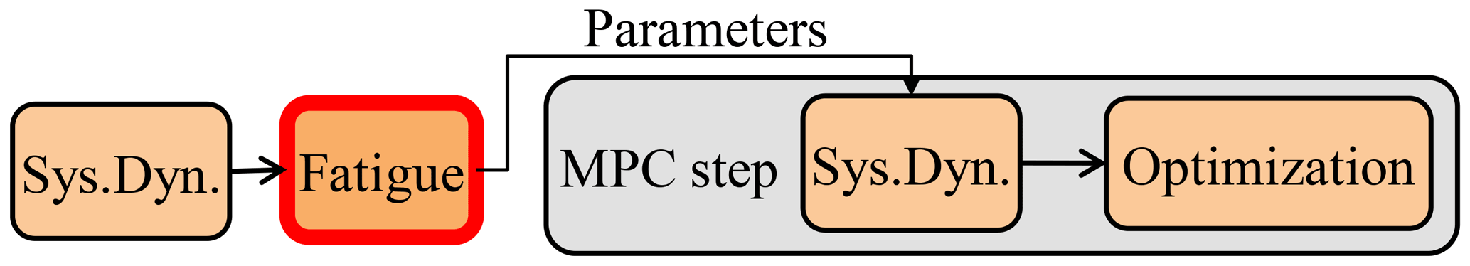
The above-mentioned obstacles for a direct implementation of RFC in MPC are overcome by the method of parametric online rainflow counting (PORFC). In PORFC, all discontinuous parts of the fatigue estimation procedure are carried out before each execution of the MPC algorithm, as shown in Fig. 2. Additionally, the stress history is incorporated via a residue, which is inspired by the batchwise cycle identification in Sect. 2.3. The algorithmic workflow is as follows.

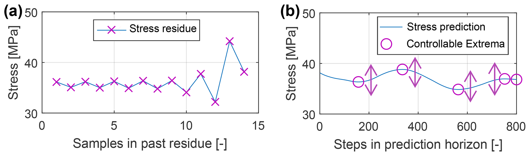
• Simulation. The reduced wind turbine model is simulated over the prediction horizon using the current measured states as initial values to produce a stress prediction, as visualized in Fig. 3b.

• Merge. The residue (see Fig. 3a) is merged with the stress prediction.

• Rainflow. The rainflow algorithm is used to identify stress cycles over this merged trajectory. Consequently, it is assumed that the structure of identified cycles does not change within the next optimization. The term “structure” denotes here positions (k_min, c, k_max, c) and weights (w_c) of cycles. As shown in Fig. 3b, this assumption implies that the controllable extrema in the prediction horizon only can be shifted vertically (i.e., in the values but not in their positions) by the optimization.

• Residue update. Stress cycles can be composed by stress samples only from residue or prediction or by a combination of both (“mixed cycle”). However, only the samples within the prediction horizon can be controlled by the optimization. Particularly the measured initial value at prediction step 0 cannot be controlled and, therefore, is added to the residue. If a full cycle is detected entirely within the residue, both contributing values are discarded from the residue. The reason for this is that also in the future they will never again form a cycle with a sample from the prediction and, therefore, are irrelevant for the MPC.

• Time-varying parameters. Information from cycle identification is used to fill vectors of time-varying parameters, which are forwarded to the cost function of the MPC. Details on this step are provided in Sect. 3.4.

• Optimization/MPC. In the cost function of the MPC, the parameters are used to time-continuously calculate fatigue cost over the horizon and accumulate it via integration. Finally, the optimization problem is solved, and the resulting control variables are applied to the wind turbine plant.

Figure 2 Externalization of fatigue estimation (Rainflow algorithm) from the MPC.

Figure 3 Stress residue from the past (a). Stress prediction into the future (b).

3.4 Parametric online rainflow counting – time-varying parameters and cost function

3.4.1 Distribution of damage over time

Since information from cycle identification is forwarded to the MPC via parameters, which are varying over the prediction horizon, the total fatigue damage has to be distributed over the prediction horizon, as visualized in Fig. 4b. Therefore, the damage of each stress cycle is split into two halves, which are allocated to the two contributing stress samples. For example, cycle 4 is formed by samples k=4 and k=8. Their fatigue cost terms therefore are allocated to these samples, as shown by the blocks in Fig. 4b. This example also shows an important property of the Rainflow algorithm, which identifies cycle 4 even though it is interrupted by the nested cycle 2, as shown in Fig. 4a. If, for a given stress sample, the complementary stress sample is not controllable (i.e., lies in the residue), all damage is allocated to the given sample. Here, this is the case for cycles 1 and 3, in which all damage is allocated to sample k=2 and k=4, respectively.

3.4.2 Setup of the time-varying parameters

Figure 4a visualizes the generation of the time-varying parameters. Since each stress extremum belongs to one or two stress cycles (Shi et al., 2018), one or two stress references are set per extremum. These stress references are considered as optimization or tracking references for the current MPC step. If both stress samples of a cycle lie in the prediction, mean stresses (M2, M4) become the stress references. If the complementary stress sample of a cycle lies in the uncontrollable residue (“mixed cycle”), this complementary stress value (C1, C3) becomes the stress reference for the considered sample in the controllable prediction. However, in many cases, a mixed cycle is crossing the level of the initial stress σ(t₀). In this case, the best possible tracking reference is this initial stress value itself (R1, R3) since zero oscillation in the prediction corresponds to zero fatigue cost. A more detailed derivation and explanation can be found in Loew et al. (2020a).

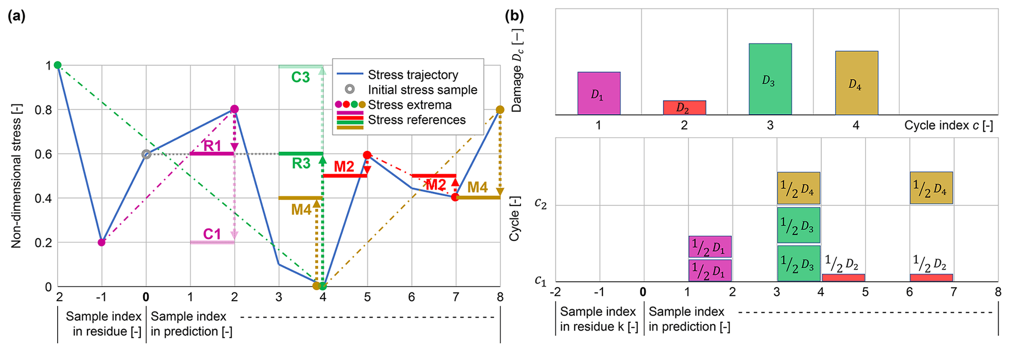
Figure 4 Stress trajectory (blue), its initial value at t₀ (grey circle), its extrema (colored dots), sequence of samples that form a cycle (dash-dotted), generated time-varying reference stresses (solid purple, red, green, yellow), and optimization goals (dotted arrows) for PORFC (a). Corresponding distribution of damage over the prediction horizon (b). Both figures are modified from Anand (2020).

3.4.3 Cost function

The fatigue cost function is defined by an integral over two cost terms, each one representing one potential cycle contribution of a stress sample, i.e.,

$$\begin{array}{}\text{(4)}& \begin{array}{rl}& J_{\mathrm{fatigue},\mathrm{PORFC}}\left(\mathit{\sigma },\stackrel{\mathrm{‾}}{\mathit{p}}\right)=\\ & {\displaystyle \frac{\mathrm{1}}{T_{\mathrm{cntrl}}}}\underset{t_{\mathrm{0}}}{\overset{t_{\mathrm{end}}}{\int }}\left(J_{\mathrm{fatigue},c}\right(\mathit{\sigma }\left(t\right),{\widehat{\stackrel{\mathrm{‾}}{\mathit{\sigma }}}}_{\mathrm{ref},c\mathrm{1}}\left(t\right),{\widehat{\stackrel{\mathrm{‾}}{w}}}_{c\mathrm{1}}\left(t\right))+\\ & J_{\mathrm{fatigue},c}\left(\mathit{\sigma }\right(t),{\widehat{\stackrel{\mathrm{‾}}{\mathit{\sigma }}}}_{\mathrm{ref},c\mathrm{2}}(t),{\widehat{\stackrel{\mathrm{‾}}{w}}}_{c\mathrm{2}}(t\left)\right))\mathrm{d}t\text{[EUR]}.\end{array}\end{array}$$

The notation $\widehat{(\cdot )}$ means fixed for one MPC step, while $\stackrel{\mathrm{‾}}{(\cdot )}$ means sampled on the control intervals of the prediction horizon. The cost terms are “switched on” by nonzero cycle weights ${\widehat{\stackrel{\mathrm{‾}}{w}}}_{c\mathrm{1}/\mathrm{2}}\left(t\right)$. Reference stresses ${\widehat{\stackrel{\mathrm{‾}}{\mathit{\sigma }}}}_{\mathrm{ref},c\mathrm{1}/\mathrm{2}}\left(t\right)$ and cycle weights ${\widehat{\stackrel{\mathrm{‾}}{w}}}_{c\mathrm{1}/\mathrm{2}}\left(t\right)$ are collected in the parameter vector,

$$\begin{array}{}\text{(5)}& \stackrel{\mathrm{‾}}{\mathit{p}}=\left(\begin{array}{c}{\widehat{\stackrel{\mathrm{‾}}{\mathit{\sigma }}}}_{\mathrm{ref},c\mathrm{1}},{\widehat{\stackrel{\mathrm{‾}}{\mathit{\sigma }}}}_{\mathrm{ref},c\mathrm{2}},{\widehat{\stackrel{\mathrm{‾}}{w}}}_{c\mathrm{1}},{\widehat{\stackrel{\mathrm{‾}}{w}}}_{c\mathrm{2}}\end{array}\right),\end{array}$$

which is defined as piecewise constant over the control intervals of the prediction horizon. The cost of individual cycles is defined by

$$\begin{array}{}\text{(6)}& J_{\mathrm{fatigue},c}={\widehat{\stackrel{\mathrm{‾}}{w}}}_{c\mathrm{1}/\mathrm{2}}\left(t\right)a_{\mathrm{m}}\left|\mathit{\sigma }\right(t)-{\widehat{\stackrel{\mathrm{‾}}{\mathit{\sigma }}}}_{\mathrm{ref},c\mathrm{1}/\mathrm{2}}(t){|}^m,\end{array}$$

where the fatigue coefficient a_m and the fatigue exponent m are derived from the damage curve of Eq. (2).

3.5 Optimization problem for TTVP and PORFC

The rigorous inclusion of fatigue into an MPC formulation described up to now is completely general and can be used to formulate different cost functions. The same formulation can be readily adjusted to include fatigue damage as an MPC constraint.

To exemplify the use of PORFC in a practical case, here the following economic optimization problem is considered:

$$\begin{array}{}\text{(7)}& \begin{array}{rl}& \underset{\stackrel{\mathrm{‾}}{\mathit{u}},\stackrel{\mathrm{‾}}{\mathit{s}}}{min}(-{\mathit{\alpha }}_{\mathrm{revenue}}{J}_{\mathrm{revenue}}+{\mathit{\alpha }}_{\mathrm{fatigue}}{J}_{\mathrm{fatigue}}+\\ & \underset{t_{\mathrm{0}}}{\overset{t_{\mathrm{end}}}{\int }}({\mathrm{10}}^{-\mathrm{1}}{\dot{\mathit{\beta }}}_{\mathrm{b}}^{\mathrm{2}}+{\mathrm{10}}^{-\mathrm{2}}{\dot{T}}_{\mathrm{g}}^{\mathrm{2}}+{\mathrm{10}}^{\mathrm{7}}{\stackrel{\mathrm{‾}}{s}}_{\mathit{\omega }}^{\mathrm{2}}+{\mathrm{10}}^{\mathrm{7}}{\stackrel{\mathrm{‾}}{s}}_{\mathrm{P}}^{\mathrm{2}})\mathrm{d}t).\end{array}\end{array}$$

The problem seeks the maximization of the revenue J_revenue and the minimization of the fatigue J_fatigue, which is represented by Eq. (3) for TTVP and Eq. (4) for PORFC. The constants α_revenue and α_fatigue are weighting factors. Instead of generated electrical energy, harvested aerodynamic energy J_revenue is maximized to avoid a greedy extraction of rotor kinetic energy by the MPC (“turnpike effect”), as suggested by Gros and Schild (2017). Furthermore, pitch rate ${\dot{\mathit{\beta }}}_{\mathrm{b}}$, torque rate ${\dot{T}}_{\mathrm{g}}$, and slack variables for rotational speed ${\stackrel{\mathrm{‾}}{s}}_{\mathit{\omega }}$ and generator power ${\stackrel{\mathrm{‾}}{s}}_{\mathrm{P}}$ are penalized (see their use in the constraints below). The optimization variables are the demanded pitch angle and torque rate $\stackrel{\mathrm{‾}}{\mathit{u}}=({\stackrel{\mathrm{‾}}{\mathit{\beta }}}_{\mathrm{b},\mathrm{d}},{\stackrel{\mathrm{‾}}{\dot{\mathit{T}}}}_{\mathrm{g},\mathrm{d}})$, as well as the slack variables $\stackrel{\mathrm{‾}}{\mathit{s}}=({\stackrel{\mathrm{‾}}{\mathit{s}}}_{\mathit{\omega }},{\stackrel{\mathrm{‾}}{\mathit{s}}}_{\mathrm{P}})$. For both TTVP and PORFC, revenue is weighted by the current electricity price α_revenue=p_elec [EUR W⁻¹ s⁻¹] to match the monetary nature of Eq. (4). The fatigue weight α_fatigue remains free and will be determined later in this work.

It should be noted that the balance of revenue and tower fatigue, despite being common in wind turbine MPC research (Gros, 2013; Evans et al., 2015; Luna et al., 2020), does not fully reflect the true economic goals of wind turbine operators, nor does it capture the complex interrelations among power capture, damage to the various turbine components, and its effects on operation and maintenance costs, on lifetime, on actuator duty cycle, and others. Therefore, the novelty of the present contribution is on how fatigue is treated in a modern control framework and not on the specific formulation of the cost function. A more realistic industrial application should embed damage into a more complex business-oriented scenario-dependent cost function or constraint. This aspect of the problem is extremely relevant and very interesting, but it is considered as out of the scope of the present work.

The optimization problem is subject to

• the system dynamics of a reduced turbine model $\dot{\mathit{x}}=\mathit{F}\left(\mathit{x}\right(t),\mathit{u}(t),\mathit{d}(t\left)\right)$, whose six states

  $$\begin{array}{}\text{(8)}& \mathit{x}\left(t\right)=\left({\mathit{\omega }}_{\mathrm{r}}\right(t),d_{\mathrm{T}}(t),{\dot{d}}_{\mathrm{T}}(t),{\mathit{\beta }}_{\mathrm{b}}(t),{\dot{\mathit{\beta }}}_{\mathrm{b}}(t),T_{\mathrm{g}}(t){)}^T\end{array}$$

  are rotational speed of the rotor noted ω_r, tower tip deflection d_T, tower tip velocity ${\dot{d}}_{\mathrm{T}}$, pitch angle β_b, pitch rate ${\dot{\mathit{\beta }}}_{\mathrm{b}}$, and generator torque T_g; more details about the model are given in Löw and Obradovic (2018);

• inequality constraints over the horizon to keep rotational speed, tower deflection (yield strength), pitch angle, pitch rate, generator torque, and generator power within their limits (in order to maintain feasibility of the optimization despite model uncertainties and temporary constraint violations, the constraints on rotational speed and generator power are augmented by slack variables, as suggested by Gros, 2013);

• box constraints on control and slack variables.

4 Moving horizon estimator

The MPC-internal system model only comprises the six states defined by Eq. (8), while the plant model in OpenFAST (including the actuators but excluding the yaw mechanism) comprises 33 states (eight tower states, six states for each of the three blades, two states for drive-shaft torsion, two states for rotor rotation, two states for the collective blade pitch actuation, one state for the generator torque actuation) (Jonkman et al., 2009). Thus, the MPC-internal model is only a reduced representation of the plant model. Furthermore, both the tower deflection and velocity of the MPC-internal model cannot be measured directly on a real turbine. Only rotor speed, tower tip fore–aft acceleration ${\ddot{d}}_{\mathrm{T}}\left(t\right)$, and the actuator states can be measured by onboard sensors. Consequently, a state estimator is required to provide initial value estimates for the MPC-internal model based on the available measurements from the plant and the lidar system.

Kalman filters are widely used for the estimation of structural wind turbine states (Bottasso and Croce, 2009; Ritter, 2020). However, they have some disadvantages compared to the more sophisticated moving horizon estimators (MHEs). First, Kalman filters are minimum-variance state estimators for linear dynamic systems with Gaussian noise; although assumptions on linearity and Gaussian noise behavior can be relaxed, MHEs are formulated as more general nonlinear optimization problems over a time horizon, which represent a natural complement to the similarly general nonlinear optimization-based formulations behind MPCs. Second, the inclusion of constraints in state estimation problems can be important to prevent non-physical results. The inclusion of state constraints is possible in Kalman filters, but not straightforward, and nonlinear constraints lead to loss of optimality of the filter and may generate different results, depending on the formulation (Simon, 2010). In contrast, state constraints can be explicitly and readily set in an MHE (Rawlings et al., 2017). Although state constraints are not employed in the estimator used in the present work, this feature may become relevant in future research. Third, Kalman filters are one-step recursive estimation methods and thus have to start operation with only one measurement time sample. In the case of large initial state errors, this can lead to inaccurate estimation and possibly to the divergence of the filter (Rawlings et al., 2017). MHEs are less vulnerable to this danger since, right from the start, they take into account an estimation horizon comprising numerous measurement samples. An advantage of the recursive nature of Kalman filters is their significantly lower computational effort compared to MHEs. However, in the present context, the computational effort of an MHE is low enough if suboptimal optimization methods such as the “real-time iteration” (Gros et al., 2013) are utilized. Because of these advantages of MHEs over Kalman filters, the former are chosen for the present work.

4.1 Formulation of the MHE

The cost function of the MHE,

$$\begin{array}{}\text{(9a)}& \begin{array}{rl}& \underset{\stackrel{\mathrm{‾}}{\mathit{v}}}{min}\underset{t_{\mathrm{0}}-T_{\mathrm{horiz},\mathrm{est}}}{\overset{t_{\mathrm{0}}}{\int }}(\Vert {\mathit{y}}_{\mathrm{est}}(t)-{\mathit{y}}_{\mathrm{meas}}(t){\Vert }_{{\mathit{W}}_{\mathrm{meas}}}^{\mathrm{2}}+\\ & \Vert {\mathit{x}}_{\mathrm{est}}\left(t\right)-{\mathit{x}}_{\mathrm{est},\mathrm{prev}}\left(t\right){\Vert }_{{\mathit{W}}_{\mathrm{prev}}}^{\mathrm{2}}+\Vert \mathit{v}\left(t\right){\Vert }_{{\mathit{W}}_v}^{\mathrm{2}})\mathrm{d}t,\end{array}\end{array}$$

penalizes differences in the current estimates from the measurements, differences in the current estimates from the previous estimates, and noise v(t) (Huang et al., 2010; Gros et al., 2013). The term x_est, prev(t) indicates the state trajectories that were estimated at the previous MHE execution, assumed as piece-wise constant and shifted backward in time by one time step. This second term of the cost function penalizes deviations over the course of consecutive MHE steps and has been added to obtain a smoother estimation output. The noise term $\stackrel{\mathrm{‾}}{\mathit{v}}$ is also assumed to be piece-wise constant. Within the vectors of estimated

$$\begin{array}{}\text{(9b)}& {\mathit{y}}_{\mathrm{est}}=\left(\begin{array}{c}{\mathit{x}}_{\mathrm{est}}\left(t\right)\\ {\ddot{d}}_{\mathrm{T},\mathrm{est}}\left(t\right)\end{array}\right)\end{array}$$

and measured variables

$$\begin{array}{}\text{(9c)}& {\mathit{y}}_{\mathrm{meas}}=\left(\begin{array}{c}{\mathit{x}}_{\mathrm{meas}}\left(t\right)\\ {\ddot{d}}_{\mathrm{T},\mathrm{meas}}\left(t\right)\end{array}\right),\end{array}$$

the states x are defined as in the reduced system given by Eq. 8. The estimated tower acceleration ${\ddot{d}}_{\mathrm{T},\mathrm{est}}\left(t\right)$ is obtained by the nonlinear output equation

$$\begin{array}{}\text{(9d)}& {\ddot{d}}_{\mathrm{T},\mathrm{est}}\left(t\right)={\displaystyle \frac{\mathrm{1}}{m_{\mathrm{T}}}}\left(F_{\mathrm{T}}\left(t\right)-c_{\mathrm{T}}{\dot{d}}_{\mathrm{T},\mathrm{est}}\left(t\right)-k_{\mathrm{T}}{d}_{\mathrm{T},\mathrm{est}}\left(t\right)\right),\end{array}$$

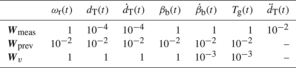
with lumped tower mass m_T, damping c_T, and stiffness k_T. The diagonal weighting matrices W_meas, W_prev, and W_v will be tuned in Sect. 5.2.4.

The optimization problem is only subject to the system dynamics,

$$\begin{array}{}\text{(9e)}& {\dot{\mathit{x}}}_{\mathrm{est}}=\mathit{F}\left({\mathit{x}}_{\mathrm{est}}\right(t),{\mathit{d}}_{\mathrm{est}}(t\left)\right)+\mathit{v}\left(t\right),\end{array}$$

with the additive optimization variable represented by the process noise v(t) (Huang et al., 2010). The external input

$$\begin{array}{}\text{(9f)}& {\mathit{d}}_{\mathrm{est}}\left(t\right)=\left(V_{\mathrm{w}}\right(t),{\mathit{\beta }}_{\mathrm{b},\mathrm{d}}(t),{\dot{T}}_{\mathrm{g},\mathrm{d}}(t){)}^T\end{array}$$

comprises the lidar-estimated wind speed V_w, as well as the pitch angle β_b,d and torque rate demands ${\dot{T}}_{\mathrm{g},\mathrm{d}}$, which have been set by the MPC and thus are fixed for the present MHE step. Notably, there is no equality constraint for the initial states ${\mathit{x}}_{\mathrm{est}}(t_{\mathrm{0}}-T_{\mathrm{horiz},\mathrm{est}})$, which thus are freely varied by the optimization algorithm.

After the execution of the MHE, the terminal states at the end of the MHE estimation horizon become the initial states at the beginning of the MPC prediction horizon:

$$\begin{array}{}\text{(10)}& \mathit{x}\left(t_{\mathrm{0}}\right)={\mathit{x}}_{\mathrm{est}}\left(t_{\mathrm{0}}\right).\end{array}$$

In the present controller setup, the optimized noise v(t) of the MHE is not utilized in the MPC, and its role is limited to the improvement of the quality of the estimates by taking into account process noise (which, in this context, also includes model errors).

4.2 Initialization of the MHE

The MHE requires information about the measurements over its entire estimation horizon. Therefore, the past measurements y_meas are buffered.

As mentioned above, the tower deflection and velocity are not measured. However, the MHE optimization benefits from meaningful measurement values as tracking reference. Therefore, a static wind-to-tower deflection mapping is interpolated over the lidar wind estimate in order to generate a proxy tower deflection trajectory d_T, meas. Tower velocity ${\dot{d}}_{\mathrm{T},\mathrm{meas}}$ is obtained by the numerical time derivative of the deflection trajectory. These quantities are termed “lidar-based references” in the remainder of this work.

5 Simulation setup, tuning, and results

In the following, the simulation setup is presented, each element of the controller toolchain is tuned, and the simulation results are discussed.

5.1 Simulation setup

5.1.1 Plant model

Various controller formulations are tested with the National Renewable Energy Laboratory (NREL) 5 MW onshore reference turbine (Jonkman et al., 2009) in the aeroelastic simulator OpenFAST. This turbine has a hub height of 110 m and a rotor diameter D=126 m. All mechanical degrees of freedom (DOF) are activated.

5.1.2 Wind model

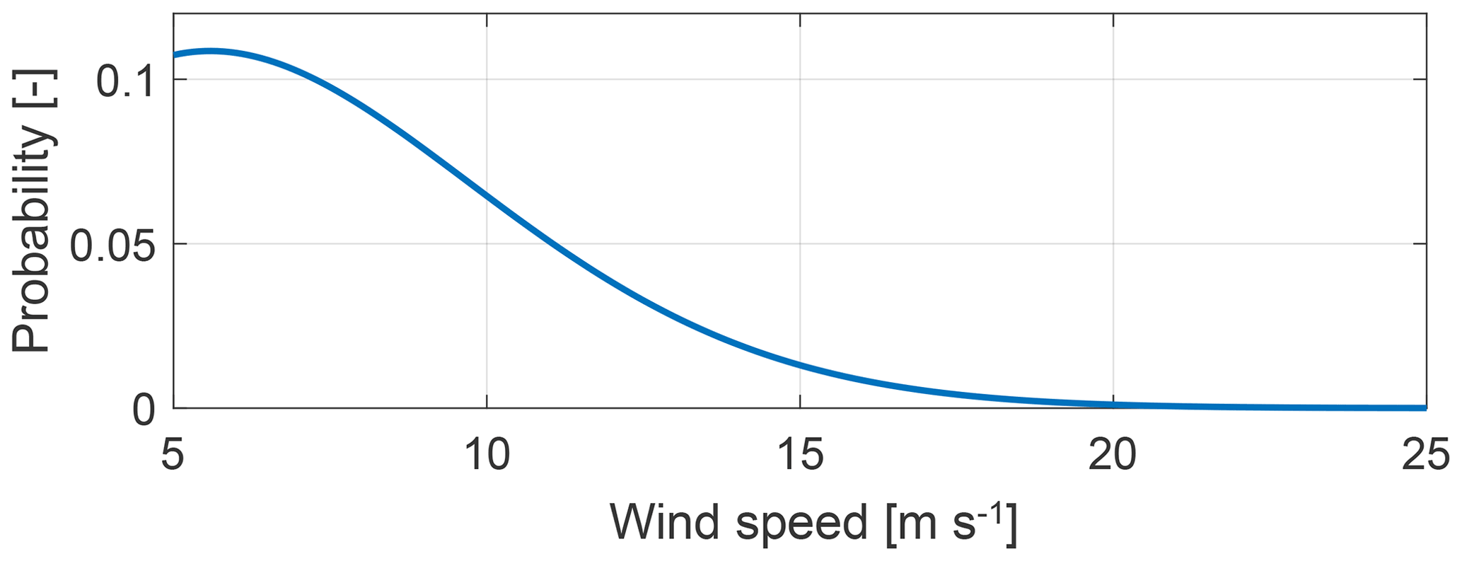
All turbulent results in this work are mean values of 12 simulations (each with a different seed) of 600 s length in DLC 1.2 with category A turbulence. For the chosen turbine with a hub height of 110 m and coastal onshore setting, a mean annual wind speed of $V_{\mathrm{w},\mathrm{mean}}=\mathrm{7}$ m s⁻¹ can be assumed (Hau, 2017). Thus, in the turbulent simulations the probability of wind speed is assumed to follow the Rayleigh distribution

$$\begin{array}{}\text{(11)}& p\left(V_{\mathrm{w}}\right)={\displaystyle \frac{\mathit{\pi }}{\mathrm{2}}}\left({\displaystyle \frac{V_{\mathrm{w}}}{V_{\mathrm{w},\mathrm{mean}}^{\mathrm{2}}}}\right)\exp \left[-{\displaystyle \frac{\mathit{\pi }}{\mathrm{4}}}{\left({\displaystyle \frac{V_{\mathrm{w}}}{V_{\mathrm{w},\mathrm{mean}}}}\right)}^{\mathrm{2}}\right],\end{array}$$

as shown in Fig. 5. The Rayleigh distribution is a variant of the Weibull distribution with the simplification of having only a single parameter (Manwell et al., 2002).

Figure 5 Rayleigh probability density function for a mean wind speed of $V_{\mathrm{w},\mathrm{mean}}=\mathrm{7}$ m s⁻¹.

5.1.3 Lidar simulator

The model of a pulsed lidar with four beams is employed. The model is implemented in the lidar simulator from sowento GmbH, which generates lidar wind estimates offline, and thus independently from the wind turbine simulation suite (Raach and Schlipf, 2018). Considered physical effects are the limitation to line-of-sight wind speeds, spatial averaging via a Gaussian range weighting function, discrete scanning, and “unfrozen” wind evolution. Particularly the wind evolution can be parameterized by an exponential decay constant; here, a higher value results in higher variation in the wind during its convection towards the rotor. Finally, the spatially distributed measurements are converted to rotor-effective wind speed by wind field reconstruction.

5.1.4 MHE and MPC framework

The MHE and MPC are implemented in the state-of-the-art acados framework (Verschueren et al., 2021), using the interior-point solver HPIPM for the underlying quadratic programs (QPs).

5.1.5 Controller variants

In the following, the performance of five MPC formulations and the baseline conventional controller (CC) from NREL (Jonkman et al., 2009) are compared. The MPCs involve the conventional formulation of TTVP (see Sect. 3.1) and the novel formulation of PORFC (see Sect. 3.3). For PORFC, a fatigue exponent of m=2 (see Eq. 6) is utilized that, resulting in quadratic cost functions, is particularly suited for quadratic programming. This case is assessed in combination with (named PORFC-2R) and without (named PORFC-2) the use of residue. Additionally, a fatigue exponent of m=5 is also tested (named PORFC-5) because this value is present at low stress amplitudes in the actual S–N curve of the tower material. However, this parameterization in combination with residue (which would be named PORFC-5R) has not led to satisfactory results and thus is not considered further.

5.1.6 Performance indicators

Considered performance indicators are revenue (analogous to energy), fatigue cost derived from damage at tower base (based on tower capital expenditures (CAPEX) and a realistic piecewise S–N curve), a simplified definition of profit (revenue minus fatigue cost), pitch travel, and torque travel. It should be noted that these definitions of fatigue cost and profit have various limitations:

• A change in tower damage can have further implications, e.g., on maintenance costs, which are not considered here.

• Changes in the pitch and torque utilization affect fatigue on other components, such as the blades and drivetrain, an effect that is not considered here.

• The computation of the actual profit of the operator is potentially much more complex and scenario-dependent than the simple model considered here.

However, the focus of the present work is on the demonstration of the rigorous inclusion of fatigue in an MPC framework rather than the solution of a realistic business case. Therefore, the results shown here should not be interpreted as being capable of providing business-critical decision support.

Another important remark is that the standard baseline CC is based on a controller design whose major objective has been neither the reduction of fatigue nor the maximization of a profit metric. Therefore, benefits of the MPCs with respect to the CC in regard of these metrics are to be expected and should not be considered as key findings of the present work. This CC is utilized here because it has been used for similar comparisons in previous publications (Schlipf et al., 2013; Luna et al., 2020) and therefore allows for some cross-comparisons to these other works. The more sophisticated – and thus relevant – comparison controller formulation is the TTVP MPC, which also has been utilized in other publications (Schlipf et al., 2013; Gros et al., 2013; Luna et al., 2020).

5.2 Tuning

Each element of the controller toolchain (lidar simulator, lidar processing, moving horizon estimator, model predictive controller) comprises a set of tunable parameters, which all impact the control performance. A comprehensive overview of these parameters is provided in Schlipf et al. (2018). Instead of tuning all parameters at once (monolithic approach), the sequential approach of Schlipf et al. (2018) is pursued. Here, the elements are tuned sequentially according to their individual performance criteria.

5.2.1 Tuning of lidar simulator

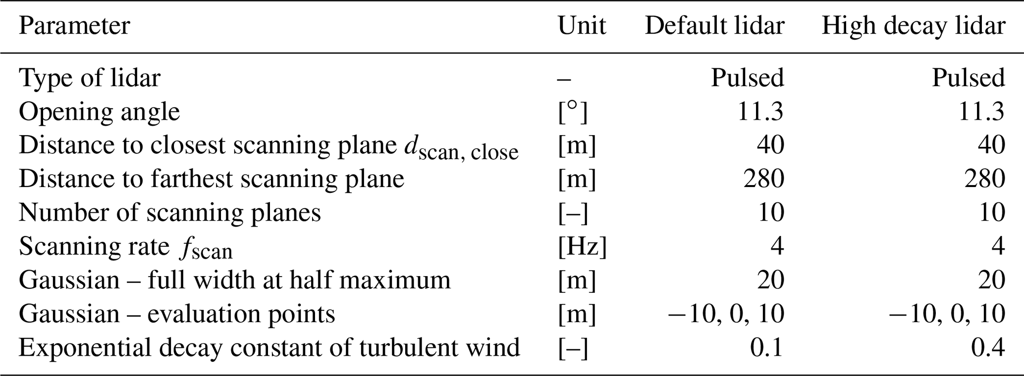
In Schlipf et al. (2018), the same wind turbine plant model (NREL 5 MW onshore) and lidar simulator are used as in the present work. There, the parameters of the lidar simulator are tuned in order to maximize the measurement coherence bandwidth for the rotor-effective wind speed. In other words, the smallest detectable eddy size is maximized, reaching a value of $D_{\mathrm{eddy},\min }=\mathrm{1.58}D=\mathrm{199}$ m. Since control of fatigue – and not lidar tuning – is the focus of the present work, the parameters of the lidar simulator in Table 1 are adopted from Schlipf et al. (2018). This “default lidar” scenario with a low decay constant of 0.1 is accompanied by a “high decay lidar” scenario, in which the exponential decay constant is increased to 0.4 (Schlipf, 2016).

Table 1 Parameters of lidar simulator for the “default lidar” and “high decay lidar” scenarios.

5.2.2 Tuning of lidar processing

The raw rotor-effective wind speed from the lidar simulator has to be buffered in order to compensate for time delays and filtered to remove uncorrelated high-frequency information. The buffer and filter parameters have to be tuned. In Schlipf et al. (2018), the tuning of the lidar processing is performed using the reduced wind turbine model as the plant model for performance reasons. However, simulations in Loew et al. (2019) have shown that unrealistically high fatigue reduction is possible if the MPC-internal and the plant models are matching. Thus, in the present work, the mid-fidelity OpenFAST model is used for tuning the lidar processing in order to benefit from its more realistic fatigue behavior.

Buffering

Inspired by Schlipf (2016), the raw rotor-effective wind speed is buffered by an adaptive buffer time span of

$$\begin{array}{}\text{(12)}& T_{\mathrm{buffer}}\left(t\right)=T_{\mathrm{travel}}\left(t\right)-\mathrm{0.5}{T}_{\mathrm{scan}}-T_{\mathrm{filter}}.\end{array}$$

Here, the traveling time $T_{\mathrm{travel}}\left(t\right)=d_{\mathrm{travel}}\left(t\right)/V_{\mathrm{mean}}\left(t\right)$ from the closest scanning plane to the rotor is obtained by the traveling distance d_travel and the current mean wind speed V_mean. The traveling distance $d_{\mathrm{travel}}\left(t\right)=d_{\mathrm{scan},\mathrm{close}}+d_{\mathrm{T}}\left(t\right)$ is the nominal distance corrected by the current tower tip deflection. The total scan time $T_{\mathrm{scan}}=\mathrm{1}/f_{\mathrm{scan}}$ is obtained from the scanning rate. The filter delay T_filter is zero here since a zero-phase filter is utilized.

Filtering

Since the lidar correlation varies with wind speed (Schlipf, 2016), the uncorrelated high-frequency information has to be processed by a low-pass filter, which is adaptive as well. In order to avoid the above-mentioned filter-delay compensation, only zero-phase algorithms have been considered. Particularly, a zero-phase forward–backward infinite impulse response (IIR) filter based on a first-order Butterworth filter (function filtfilt in MATLAB) has been compared to a central moving mean filter (function movmean in MATLAB). For this purpose, the lidar simulator parameterization from Sect. 5.2.1 and a reasonable initial parameterization of the MHE and MPC have been utilized in turbulent simulations. Despite its simplicity, with different MPC formulations and horizon lengths, the moving mean filter has exhibited superior performance and thus has been chosen for the present application. It should be noted that this superiority of the moving mean filter has only been observed for the present lidar and wind turbine configuration and cannot be generalized. Thus, for another configuration, the comparison should be repeated. Beneficially, the moving mean filter only requires tuning of its window length. The empirical formula

$$\begin{array}{}\text{(13)}& T_{\mathrm{movmean}}\left(t\right)={\displaystyle \frac{D_{\mathrm{eddy},\min }}{V_{\mathrm{mean}}\left(t\right)}},\end{array}$$

which is based on the smallest detectable eddy size and the current mean wind speed, has led to a very good adaptive tuning for the present setup.

Due to its nature, the central moving mean filter requires sufficient information from the past and future. Except for the beginning of a simulation, the amount of past information is typically sufficient and even growing in the course of the simulation. In contrast, sufficient future information beyond the prediction horizon is only ensured if the inequality

$$\begin{array}{}\text{(14)}& T_{\mathrm{pred}}\left(t\right)-\mathrm{0.5}{T}_{\mathrm{movmean}}\left(t\right)\ge T_{\mathrm{horiz}}\end{array}$$

holds, where half the moving mean filter length T_movmean subtracted from the lidar-predicted time T_pred exceeds the MPC horizon length T_horiz. The lidar-predicted time $T_{\mathrm{pred}}\left(t\right)=d_{\mathrm{scan},\mathrm{far}}/V_{\mathrm{mean}}\left(t\right)$ depends on the distance of the farthest scanning plane to the rotor and the current mean wind speed. As shown in Fig. 6, the inequality typically holds and is only slightly violated at V_mean>22 m s⁻¹.

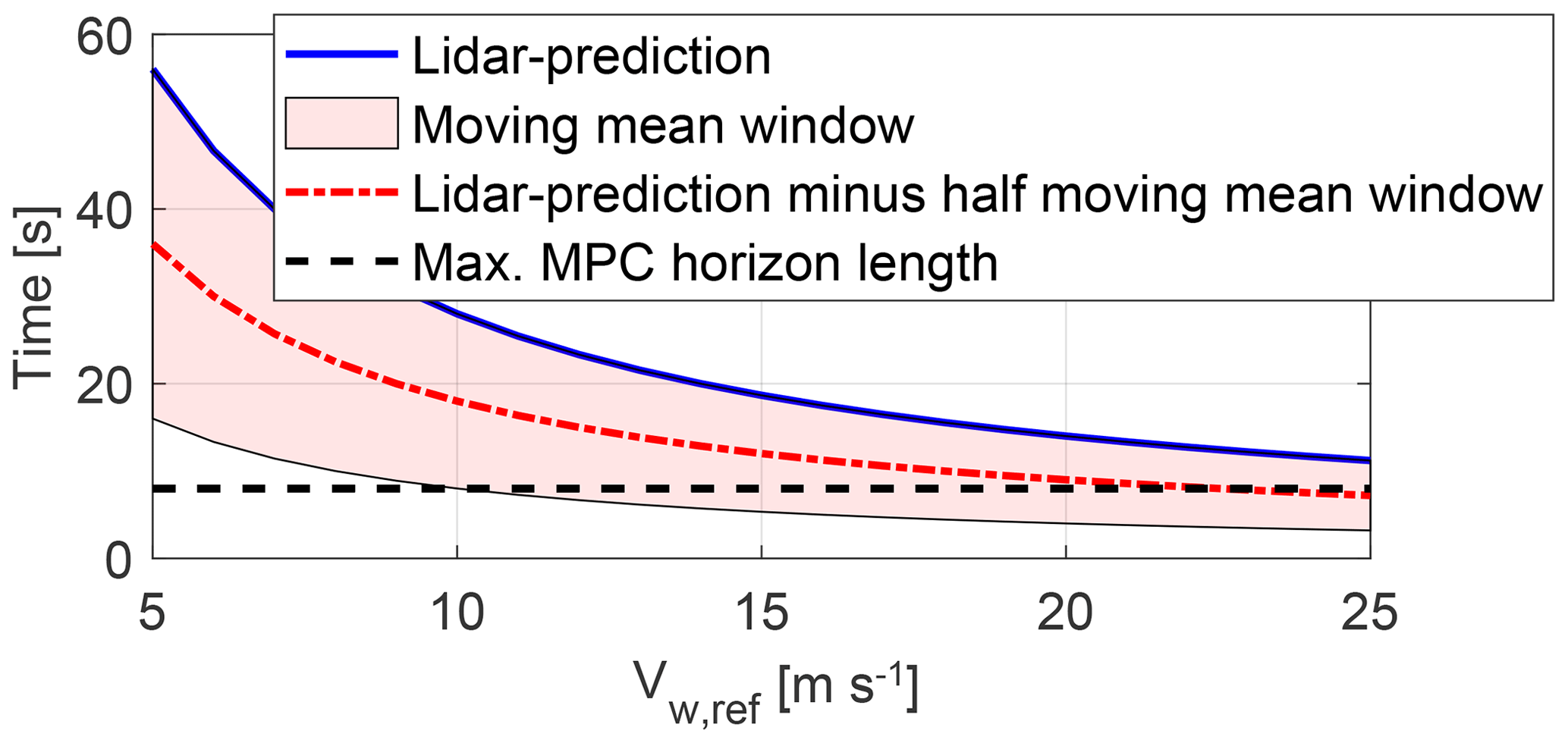
Figure 6 Comparison of the effectively available filtered prediction information (dash-dotted red) to the MPC horizon length (dashed black).

Further scaling of buffer and filter parameters

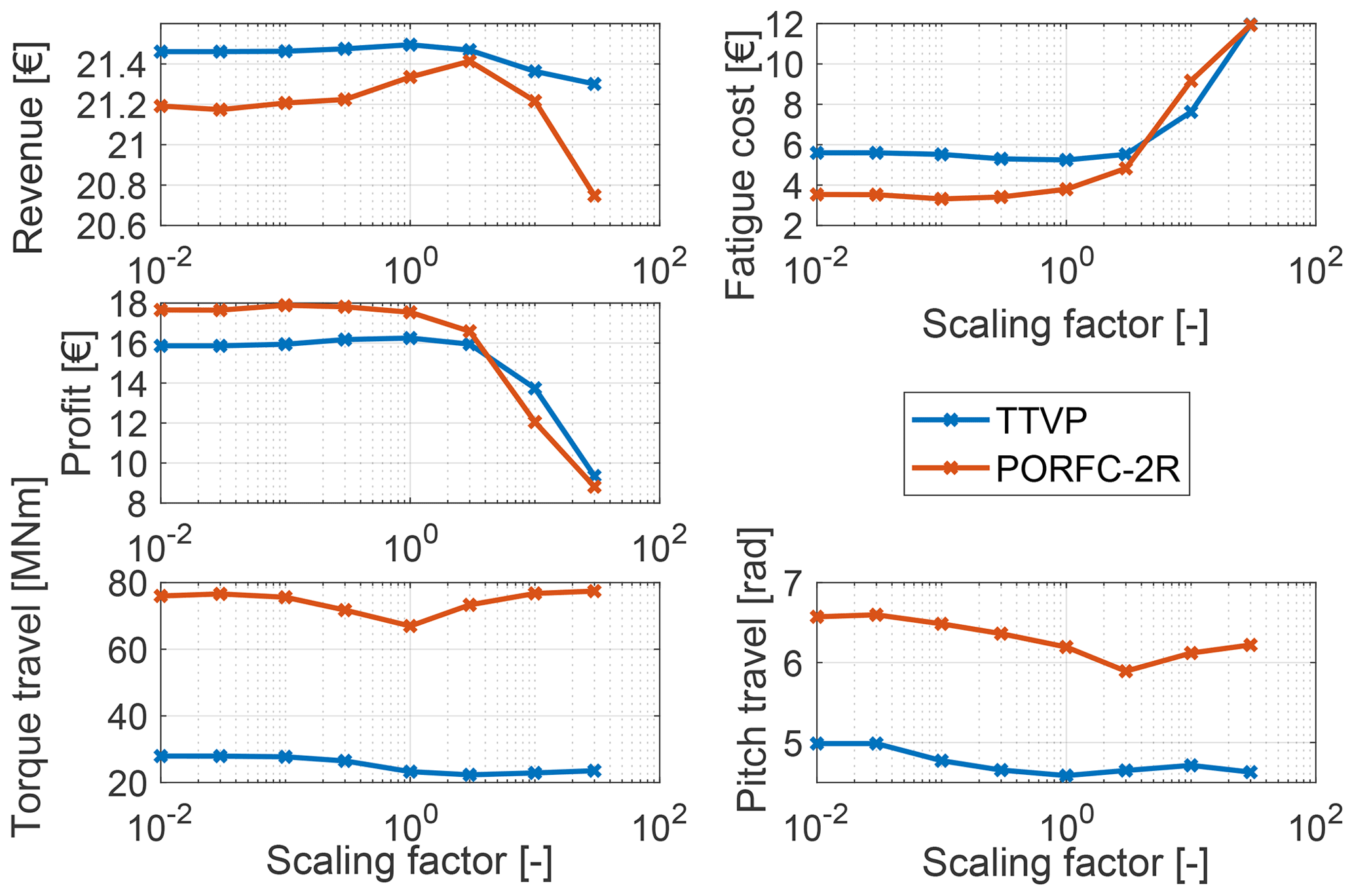
In order to verify the above adaptation formula, simulations have been executed in which these buffer and filter window lengths are increased or decreased. These results are generated for the “high decay lidar” scenario, in which lidar data quality is lower, and thus correct filtering is more important. The simulations reveal that the above adaptation laws lead already to high revenue and low fatigue cost. As shown for the filter window length in Fig. 7, for both TTVP and PORFC with scaling factors of 1, a high revenue is maintained while achieving low fatigue cost. Lower scaling factors (shorter filter windows) have a tendency towards higher actuator usage, while higher scaling factors dramatically increase fatigue cost. Consequently, scaling of the buffer and filter parameters is not applied in the present work.

Figure 7 Variation in KPIs depending on the scaling of moving mean filter window length.

5.2.3 Tuning of the MHE algorithm

The MHE is set up with an estimation horizon length of 8 s and a sample time of 0.1 s, which are fixed for all MPC configurations.

5.2.4 Tuning of the MHE cost weights

Practical experience has shown that the goal of the MHE should not be an accurate reconstruction of the unmeasured true plant states of tower tip deflection and velocity, as shown in Fig. 8. In fact, an accurate reconstruction would contain high frequencies from the plant higher-order degrees of freedom that, not being matched by corresponding degrees of freedom of the MPC-internal model, would spill over and pollute its lower-order degrees of freedom.

Instead, the MHE should provide low-frequency initial states for the low-frequency MPC-internal model (“estimated initial” states). Consequently, the MHE is tuned to estimate state trajectories that best fit the behavior of the reduced model. This is achieved by setting low weights for the tower variables in the weighting matrix W_meas, as shown in Table 2. These low weights allow for significant deviations from the measured tower acceleration and the lidar-based references and thus for a greater focus on the reduced model dynamics. For tower deflection and velocity, very low values of 10⁻⁴ are chosen since these quantities are not measured. For tower acceleration, an intermediate value of 10⁻² is chosen since it is measured, but its trajectory does not need to be tracked carefully.

The estimated tower deflection in Fig. 8 exhibits a significant steady-state offset from the unmeasured true tower deflection. This can be possibly attributed to the inaccurate system model since this offset also pertains in the MPC prediction, which is based on the same system model.

Figure 8 Wind turbine tower quantities ordered by occurrence in the estimation and control process: measured, unmeasured, lidar-based reference (see Sect. 4.2), estimated, and predicted. Negative time samples are estimation horizon of the MHE; positive time samples are prediction horizon of the MPC.

By the intermediate weights in the weighting matrix W_prev, the current state trajectories are only loosely tied to the previous ones.

In the weighting matrix W_v, significant noise is only permitted for the pitch angle and torque rate in order to enable a close match of pitch and torque estimations with their already accurate measurements.

Table 2 Diagonal elements of the weighting matrices W penalizing the corresponding entries of the estimation y_est and noise v vectors.

5.2.5 Tuning of the MPC algorithm

The controller sample time is set to 0.1 s like in Bottasso et al. (2014) and Gros and Schild (2017). The maximum horizon length of $T_{\mathrm{horiz},\max }=\mathrm{8}$ s is chosen based on the findings of Loew et al. (2020b), which indicate that a considerable portion of the plant stress cycles will be contained in this prediction horizon. However, since horizon length has a substantial impact on performance and since, moreover, the longest horizon is not always the best, shorter horizons of $T_{\mathrm{horiz}}=\mathit{\{}\mathrm{4};\mathrm{2};\mathrm{1}\mathit{\}}$ s will be tested throughout all turbulent studies.

One QP is solved per MPC step. The Hessian matrix is automatically convexified to account for possible numerical issues due to the highly non-standard cost formulation of PORFC. Practical experience has shown that performance is improved if the Newton step length of the QP is reduced from 1 to 0.1. This can be explained by the frequently changing optimization problems, especially for PORFC. In this case the initialization of the QP might not be sufficiently close to the optimum, and full Newton steps could leave the region of validity of the quadratic approximation of the nonlinear program (Diehl and Gros, 2020).

5.2.6 Tuning of the MPC cost weights

As shown in Sect. 3.5, all weights in the cost function except for the fatigue weight α_fatigue are pre-defined for simplicity. Thus, only the fatigue weight has to be tuned in the following. Tuning is executed at a single reference wind speed of $V_{\mathrm{w},\mathrm{ref}}=\mathrm{9}$ m s⁻¹. This wind speed is chosen since, for the conventional controller CC, the highest profit contribution occurs there, as shown in terms of profit density in Fig. 9. Profit density represents the incremental contribution to total cumulative profit at a certain wind speed. Other meaningful criteria for a suitable tuning wind speed would be the wind speed at which half of the total cumulative profit is reached or where the highest revenue contribution occurs.

Figure 9 Normalized profit density and cumulative profit. The latter is normalized with respect to the total profit of the conventional controller.

The variation in important key performance indicators (KPIs) with fatigue weights is shown in Fig. 10. For brevity, only the results for the maximum MPC horizon length of 8 s are shown. All variants of PORFC are able to maintain high revenue levels while decreasing fatigue cost with increasing fatigue weights. In contrast, the revenue of TTVP declines rapidly above a certain fatigue weight. Thus, the tuning of PORFC can be considered as less critical than that of TTVP. Since in most cases torque travel and pitch travel increase with fatigue weight, low fatigue weights should be preferred as long as fatigue cost is not harmed significantly. Following this strategy, the fatigue weights are determined for all controller formulations and horizon lengths, as shown in Table 3.

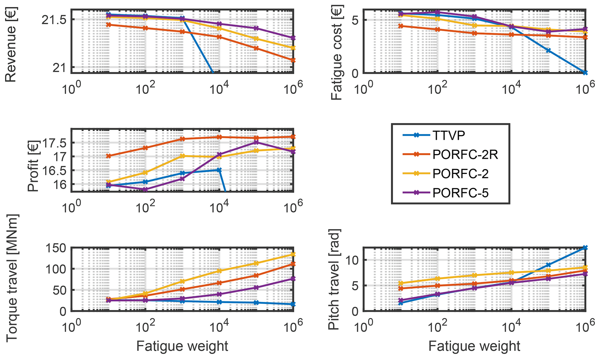
Figure 10 Variation in KPIs for different fatigue weights and a prediction horizon length of T_horiz=8 s.

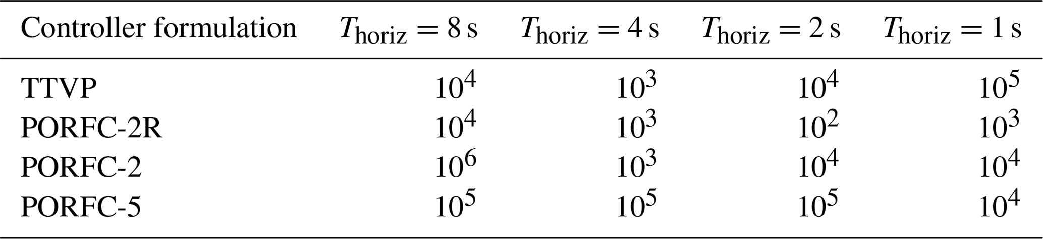
Table 3 Optimum fatigue cost weights α_fatigue for different controller formulations and prediction horizon lengths.

5.3 Results of turbulent simulations

5.3.1 Comparison of controller formulations in the “default lidar” scenario

As a next step, the optimal tuning weights from Sect. 5.2.6 are fixed, and simulations at different reference wind speeds $V_{\mathrm{w},\mathrm{ref}}=\mathit{\{}\mathrm{5};\mathrm{7};\mathrm{\dots };\mathrm{25}\mathit{\}}$ m s⁻¹ are performed for each controller formulation and prediction horizon length. The simulations result in the Weibull-weighted cumulative KPIs shown in Fig. 11.

For all MPCs, revenue is at least slightly below the one of the CC. However, especially for PORFC-2R and PORFC-5 with a prediction horizon of T_horiz≥2 s, the revenue losses remain moderate. In contrast, all MPCs with T_horiz≥2 s exhibit substantially lower fatigue cost than the CC. As a rough indication of the combined effect, the changes in revenue and fatigue cost can be assessed in terms of the simplified profit indicator. The highest profit gain is achieved by PORFC-2R at maximum prediction horizon, which surpasses CC by 30 % and the best TTVP by 2.5 %. At least for the present setting, very short horizons of 1 s cannot be recommended since they significantly decrease revenue and greatly increase fatigue.

Over different horizon lengths, PORFC-2R exhibits very stable revenue and fatigue levels. In contrast, for the PORFC formulations without residue (PORFC-2, PORFC-5), a shorter horizon of T_horiz=4 s exhibits higher profit than T_horiz=8 s. This phenomenon may be explained by a higher influence of the prediction errors: due to model errors and wind evolution, the predicted states at the end 4 s $<t\le \mathrm{8}$ s of a long horizon may be affected by large errors. Since PORFC-2 and PORFC-5 have to rely solely on the predictions, their performance may suffer from long horizons.

For all MPCs, the fatigue reduction with respect to CC comes at the price of a higher pitch travel. Here, TTVP exhibits around 6 times the pitch travel of CC. Since in the literature more moderate increases (e.g., by a factor of 2) are reported (Luna et al., 2020), further studies on pitch penalization should be conducted. For PORFC, pitch travel is even slightly higher and is somewhat reduced by a reduction in horizon length. Torque travel exhibits different behavior in that several MPC formulations have a lower torque travel than CC.

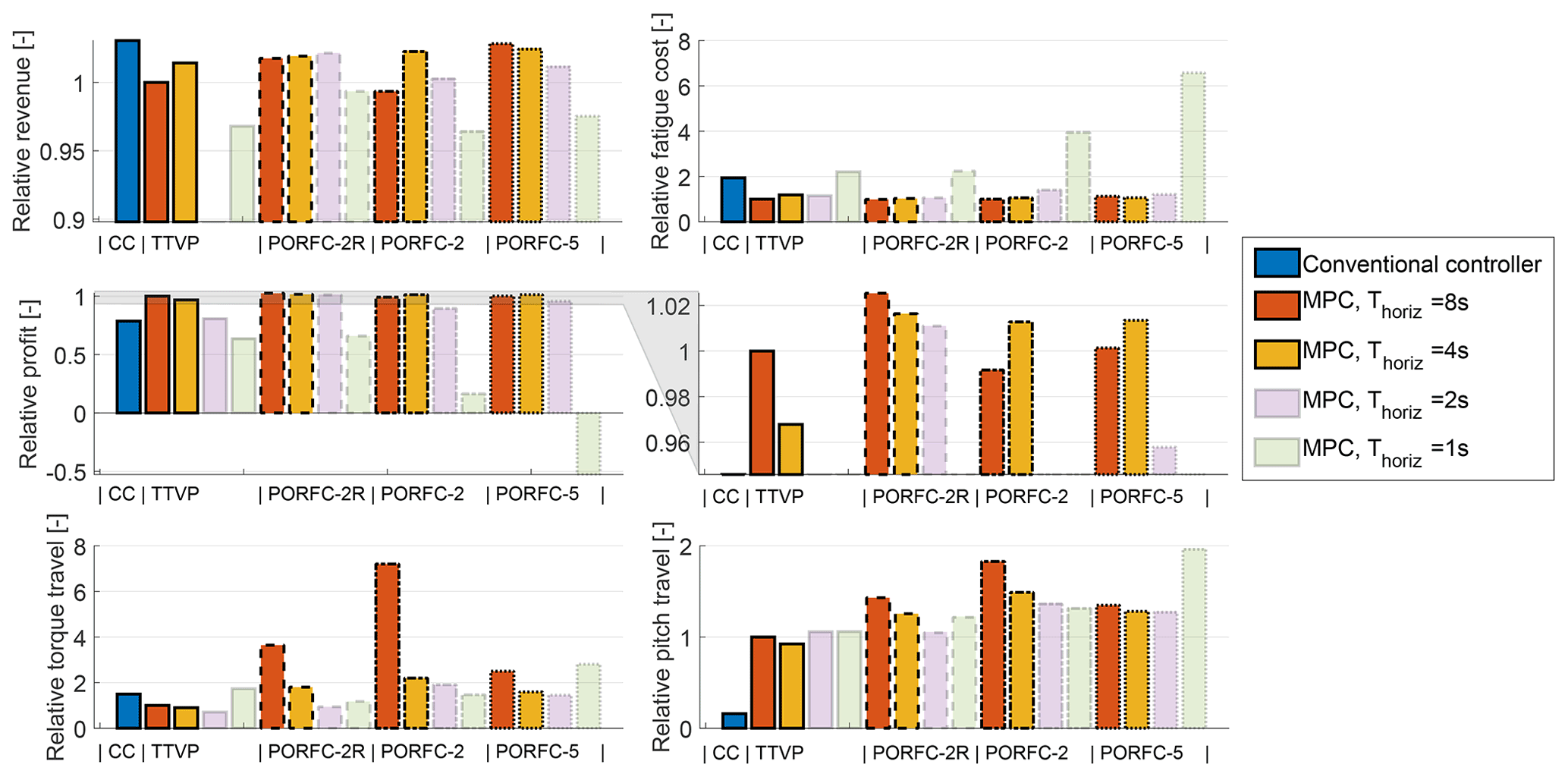
Figure 11 “Default lidar” scenario. Weibull-weighted KPIs for different controller formulations (indicated by edge style) and MPC prediction horizon lengths (indicated by color). The results for the shorter horizons are transparent in order to focus the attention on the more important longer horizons. Results are normalized with respect to the best TTVP configuration with a prediction horizon length of T_horiz=8 s. Middle row, right: zoomed version of profit plot.

A look at the profit density and cumulative profit in Fig. 9 shows that both MPC formulations (TTVP, PORFC) “earn money” very similarly over wind speed. Compared to CC, the MPC fatigue reduction strategies lead to profit benefits at very low and at intermediate wind speeds. With the present tuning, TTVP has a slight extra advantage at very low wind speeds, while PORFC-2R is superior over a broad range of intermediate wind speeds.

5.3.2 Performance in the “high decay lidar” scenario

The “default lidar” scenario of the previous sections can be considered as very favorable for lidar-assisted control since the wind does not change very much between the lidar measurement planes and the rotor. Thus, the lidar provides a fairly good estimate of the true incoming wind. In order to challenge the MPCs even more, a further assessment is performed for the “high decay lidar” scenario (see Table 1).

Despite the significant reduction in lidar signal quality, the profit benefit of the MPCs over CC decreases only slightly, as shown in Fig. 12. Particularly, the best-performing PORFC-2R (T_horiz=4 s) still surpasses CC by 26 % for the “high decay lidar” scenario, in comparison to the above-mentioned 30 % for the “default lidar” scenario.

The profit benefit of 5.1 % of the best PORFC-2R (T_horiz=4 s) over the best TTVP (T_horiz=8 s) shows that PORFC-2R is particularly strong in handling situations of low lidar data quality. In a direct comparison using the same horizon length (T_horiz=4 s), PORFC-2R is superior by almost 9 %. Just like in the “default lidar” scenario, PORFC-2R exhibits better revenue stability over the horizon lengths $T_{\mathrm{horiz}}=\mathit{\{}\mathrm{8};\mathrm{4};\mathrm{2}\mathit{\}}$ s but also exhibits excessive fatigue cost at T_horiz=1 s.

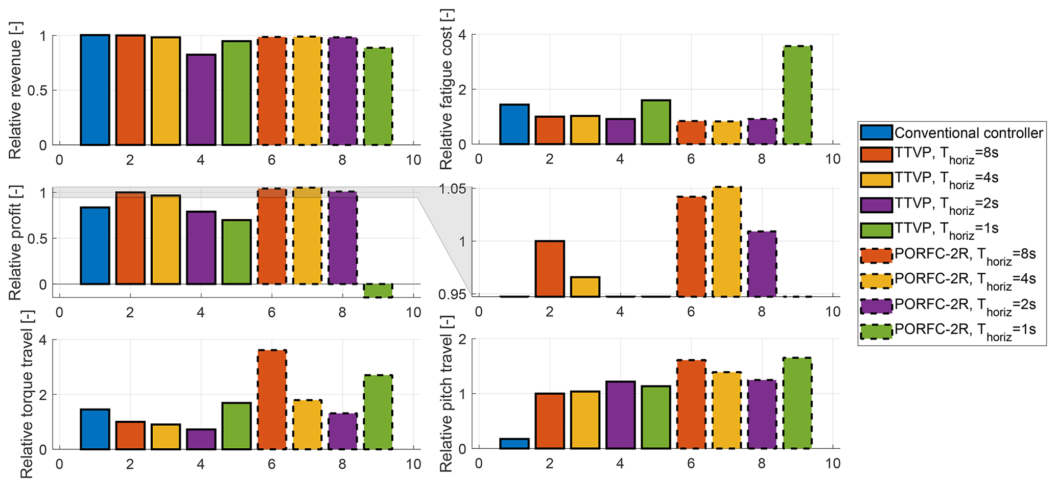
Figure 12 “High decay lidar” scenario. Weibull-weighted KPIs for different controller formulations and prediction horizon lengths. Results are normalized with respect to the best TTVP configuration with a prediction horizon length of T_horiz=8 s. Middle row, right: zoomed version of profit plot.

5.3.3 Performance in the “perfect prediction” scenario

The increasing benefit of PORFC-2R with respect to TTVP with lower lidar data quality conversely suggests decreasing benefits with very high lidar data quality. This hypothesis is actually partially confirmed by the extreme scenario of a perfect wind prediction (without lidar errors). As shown in Fig. 13, as expected, fatigue cost can be reduced by TTVP and PORFC-2R even further than in the “default lidar” scenario of Sect. 5.3.1. However, relative to TTVP, the advantage of PORFC-2R decreases significantly. For the maximum horizon length, the profit of TTVP even slightly surpasses PORFC-2R by 0.4 %. On the other hand, as revenue and fatigue cost of PORFC-2R are more stable for shorter horizons, this formulation retains a significant advantage there.

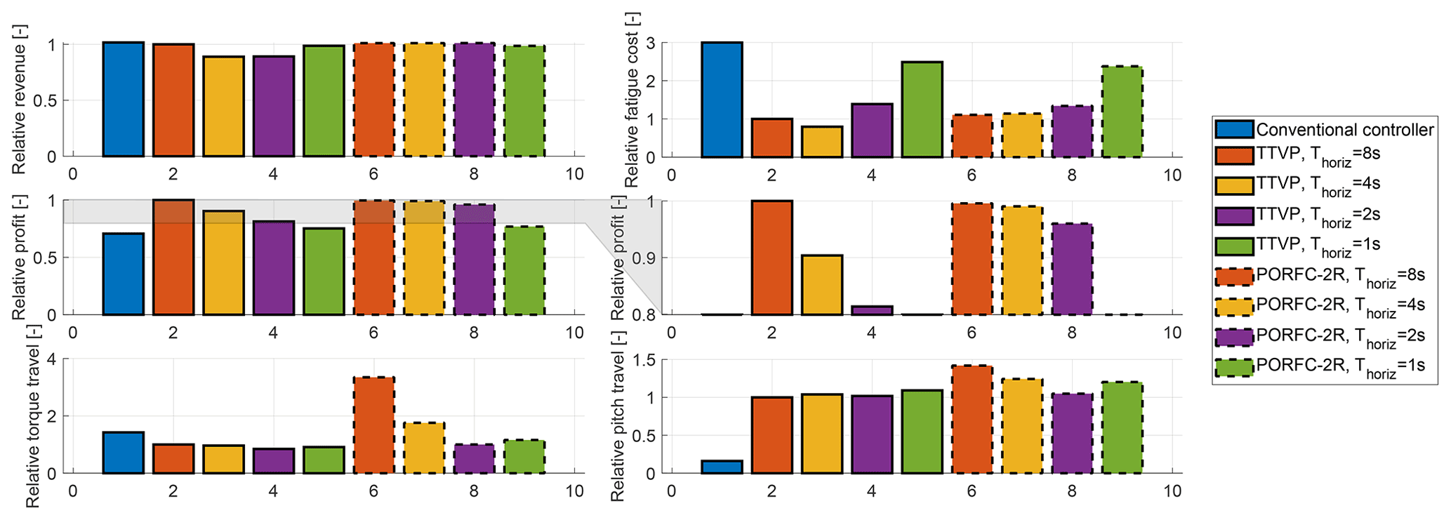
Figure 13 “Perfect prediction” scenario. Weibull-weighted KPIs for different controller formulations and prediction horizon lengths. Results are normalized with respect to the best TTVP configuration with a prediction horizon length of T_horiz=8 s. Middle row, right: zoomed version of profit plot.

5.3.4 Benefit of “perfect prediction” vs. “perfect persistence”

All previous scenarios assumed a wind preview. However, to date, lidar systems can still account for a significant portion of the capital and operational expenditures of wind turbines (Canet et al., 2020). In order to avoid lidar-related costs or effort, some studies are directed towards predictive control without explicit preview measurement (Evans et al., 2015; Jassmann et al., 2016). In this case, the wind prediction over the MPC horizon can for instance be generated via constant extrapolation of the instantaneous wind estimate at the rotor (persistence). This motivates an analysis of how the novel PORFC MPC actually benefits from a predictive preview compared to a persistent preview.

Since the design of a rotor-effective wind speed estimator is out of scope of the present work, a “perfect persistence” scenario is employed and compared to the above “perfect prediction” scenario.

As shown in Fig. 14, all MPC formulations significantly benefit from prediction (instead of persistence). For all formulations, this is primarily achieved by high fatigue reduction. At the same time, actuator usage is moderately decreased or even increased at some horizon lengths for TTVP but is significantly decreased for PORFC-2R if T_horiz≥2 s.

These results further indicate the technical benefit of lidar-assisted control and motivate further studies comparing the realistic lidar wind preview with a sophisticated wind speed estimator.

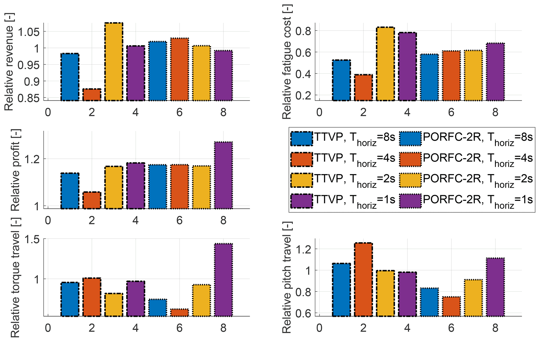
Figure 14 Weibull-weighted KPIs of the “perfect prediction” scenario normalized with respect to the individually corresponding KPIs of the “perfect persistence” scenario with the same MPC formulation and horizon length.

5.4 Insights into PORFC

In order to gain deeper insight into the behavior of PORFC, short time periods within a turbulent simulation in the “default lidar” scenario are analyzed.

5.4.1 Evolution of residue

Figure 15 shows a situation where the stress prediction at the initial value σ(t₀) turns from a mildly rising slope (MPC step 1) to a mildly falling slope (MPC step 2). Consequently, a new stress maximum is formed and added to the “right-hand side” of the residue set at MPC step 2, as shown in Fig. 15a. In the following steps 3 to 5, the size of the residue set remains constant; only the right-hand-side value is updated by the current initial stress value.

5.4.2 Evolution of PORFC parameters

As shown in Fig. 15b, the change in extrema in the stress prediction over the course of MPC steps leads to frequent changes in the PORFC stress references (see Sect. 3.4.2) or, more in general, in the PORFC parameter structure (see bars in Fig. 15b). However, since many of the emerging or vanishing stress cycles are small in amplitude, also their corresponding stress reference values are close to the stress prediction trajectory (compare bars to the solid blue line) and thus have low impact on the overall optimization problem.

Since by nature of MPC the stress trajectory is shifted to the left-hand side with each simulation step, also the PORFC parameter samples are shifted. This becomes even more clear in Fig. 16, where stress reference 1 is plotted over the prediction horizon and over MPC steps (simulation time). Here, over the course of MPC steps, the stress reference pattern is evolving smoothly towards the beginning of the prediction horizon. While some references emerge within the prediction horizon, many references originate at the end and do not vanish before reaching the beginning of the prediction horizon.

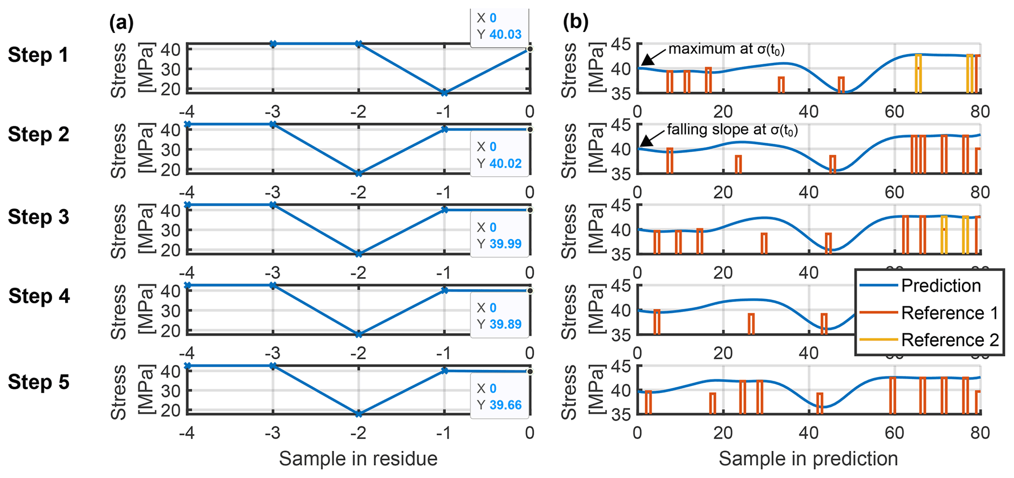
Figure 15 Stress trajectories for PORFC-2R in turbulent wind 10 s after the start of the simulation. Top-down: five consecutive MPC steps. Residue set of variable size, in which the values of the last stress samples are labeled (a). Stress prediction of the MPC and stress references as part of the PORFC parameter set (b).

Figure 16 PORFC stress reference over the prediction horizon of 80 samples for 100 consecutive MPC steps.

5.5 Results of deterministic gust simulations

According to the current standards (IEC, 2005), a central qualification criterion for controllers is their reaction to deterministic gusts. Previous literature already has shown that deterministic gusts are an easy but unrealistic task for predictive controllers like MPCs (Schlipf and Raach, 2016), resulting in too optimistic conclusions regarding extreme load reduction. Besides, extreme loads are not even always design-driving for some wind turbine components (Canet et al., 2020). Nonetheless, the study of gust scenarios sheds additional light on the controller dynamic behavior.

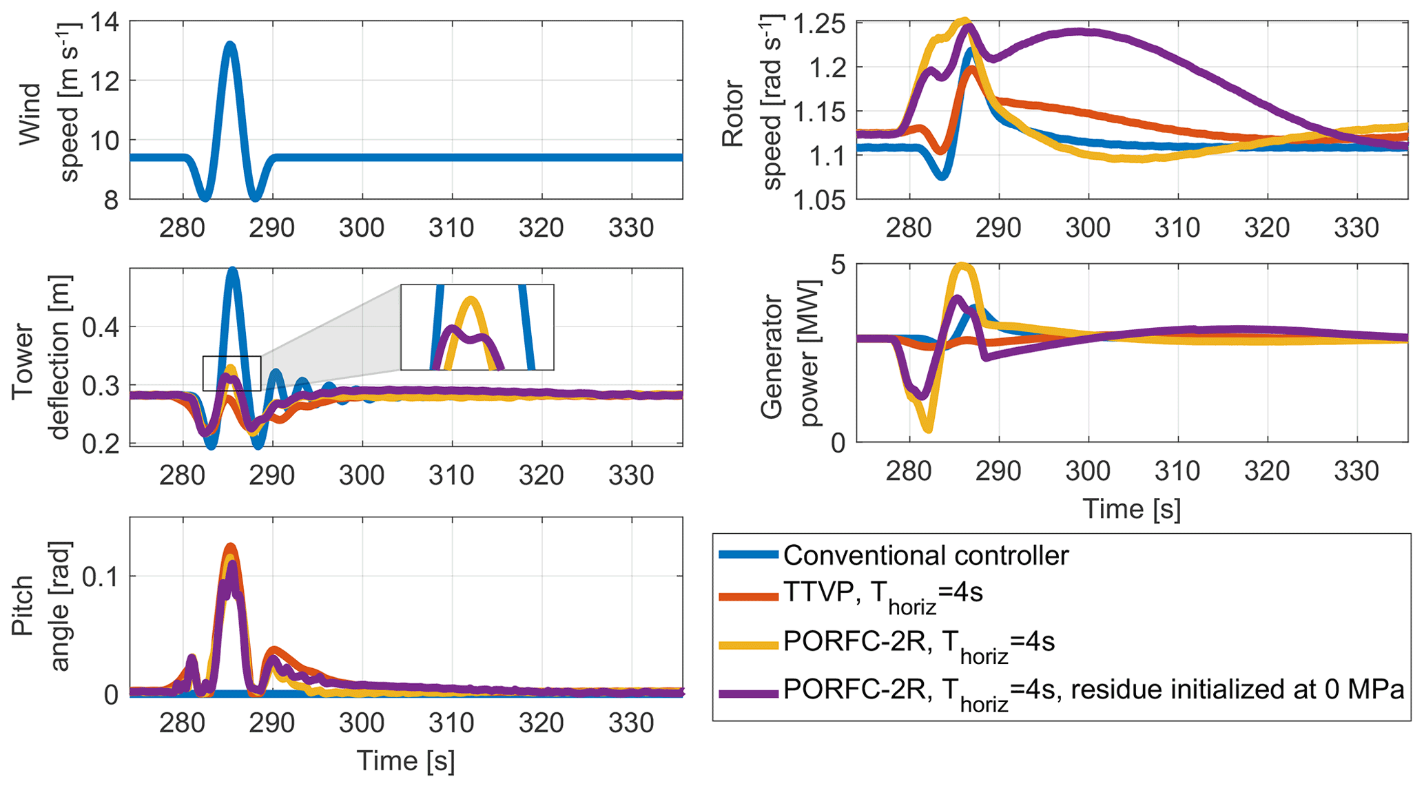
Thus, in the following, the conventional controller is compared to the MPC formulations of TTVP and PORFC-2R in an “extreme operating gust” scenario (IEC, 2005), with a duration of 10.5 s and an initial wind speed that is 2 m s⁻¹ below rated wind speed (V_rated=11.4 m s⁻¹). In order to test the MPCs with partial knowledge of the gust, a prediction horizon of 4 s is chosen. Besides this limited horizon, a perfect wind prediction without lidar errors is assumed.

As shown in Fig. 17, even during the gust, for all controllers the rotor speed remains below the rated speed of 1.267 rad s⁻¹. As a result, the conventional controller remains at the minimum pitch angle, and the tower deflection freely follows the gust wind speed, which leads to a high positive excursion. After the gust, the tower oscillation quickly vanishes due to aerodynamic damping.

In contrast, the MPCs anticipate the incoming gust and react to a significant extent by pitching the blades. Interestingly, despite their different fatigue cost formulations, the MPCs exhibit very similar pitching behavior. As expected, the TTVP and the PORFC-2R MPC attenuate very effectively the tower excursion and dampen the oscillation immediately. However, PORFC-2R puts less priority on the attenuation of the tower excursion. Since the tower deflection has been flat prior to the gust, the stress residue of PORFC-2R contains only stress values around the steady state. Consequently, PORFC-2R assumes only a small stress cycle with low damage potential during the gust. This behavior is changed if the stress residue is initialized with 0 MPa, which corresponds to an undeflected tower prior to operation. Due to this stress memory, PORFC-2R identifies a large half cycle and consequently tries to further limit the maximum tower excursion by peak shaving, as shown by the purple trajectory in Fig. 17.

Clear differences of PORFC-2R with respect to TTVP can be seen in the rotor speed and generator power dynamics. At the beginning of the gust, the generator power is reduced in order to achieve a high rotor speed during the gust. This behavior can be attributed to an attempt at harvesting the energy of the gust and also has been observed for an MPC where 5 QPs (instead of 1 QP) have been solved per MPC step for better convergence. For the PORFC-2R MPC with the 0 MPa residue, the rotor speed remains at a high level for a longer time frame, which is an unusual behavior and requires more investigation. Finally, it can be noted that the steady-state rotor speed is slightly higher for the MPCs than for the conventional controller, as seen before the gust. Assuming perfect tracking of optimal rotor speed by the conventional controller, this difference can be attributed to the MPC plant–model mismatch. However, as shown in Fig. 17, the rotor speed difference does not result in significant suboptimality of the steady-state power capture.

Figure 17 Extreme operating gust at $V=V_{\mathrm{rated}}-\mathrm{2}$ m s⁻¹.

6 Conclusions and outlook

6.1 Conclusions

The present work represents a significant step in assessing the benefits of the MPC formulation of PORFC. For this purpose, the simulation setup of Loew et al. (2020b) has been extended by a realistic lidar simulator, lidar processing, and an MHE.

First, the PORFC formulation has been presented in an application-focused way. It has been highlighted how PORFC directly incorporates mechanical fatigue in predictive wind turbine control. Since fatigue requires long observation windows, stress history has been considered in a consistent manner by carrying along a residue (PORFC-2R).

Second, the formulation of the MHE has been explained, in which the lidar wind estimate has been used to generate an initialization for the unmeasured tower states.

Third, a sequential tuning approach has been employed for the lidar simulator, lidar processing, MHE, and MPC:

• For the lidar simulator, parameters from the literature have been utilized, which maximize the measurement coherence bandwidth.

• For the lidar buffering and filtering, simple adaptive tuning laws have been employed. Simulations have revealed that they result already in good performance and that no further tuning seems to be required.

• For the MHE, instead of accurately reconstructing the plant states, the cost weights have been tuned to estimate only the low-frequency state information that can be handled by the MPC-internal model.

• For the MPC, four different prediction horizon lengths have been employed throughout the study since no single horizon length has led to the best performance in all scenarios. In the MPC cost function, the fatigue weight has been tuned systematically for each controller formulation and horizon length.

Finally, extensive economic and dynamic simulation results have been presented for turbulent and gust wind settings:

• In the “default lidar” scenario, all MPCs are able to significantly reduce fatigue cost with respect to a conventional PID controller, while PORFC-2R has to sacrifice less revenue than a conventional MPC. For shorter horizons, especially the PORFC formulation with residue has shown a more robust performance than the conventional MPC.

• In the “high decay lidar” scenario with a lower lidar prediction quality, the advantage of PORFC-2R over the conventional MPC even increases. This suggests that PORFC-2R is a recommended solution especially for lower lidar prediction quality.

• In the “perfect prediction” scenario, both MPCs have exhibited similar results. A comparison with a wind persistence setting has shown that PORFC-2R benefits more from the availability of this high-quality prediction than the conventional MPC.

• In all considered turbulent scenarios, MPCs with a very short prediction horizon of 1 s have obtained only modest results.

• An excerpt of a turbulent simulation with PORFC-2R has demonstrated how the residue is updated and that the parametric stress references evolve smoothly following an expected pattern.

• In an extreme operating gust setting, both MPCs have shown a similar pitching behavior and the effective attenuation of tower excursion. During the gust, PORFC-2R has shown a higher variability in the rotor speed.

6.2 Outlook

The MPC formulation of PORFC still has several aspects worth investigating:

• For the MHE tuning, an automated but still computationally tractable approach should be developed.

• The MHE- and MPC-internal system model has a significant error with respect to the plant system. Thus, online model adaptation promises further benefits.

• In the MPC cost function, economic terms for the actuator, blade, and drivetrain damage should be included.

• In certain business cases, the goal may not be to minimize fatigue but simply to keep the fatigue rate on average below certain thresholds or to keep the cumulative damage below a threshold by the end of service. To assist these goals, the PORFC cost function could be modified, and fatigue could be added as a parametric constraint in the MPC. Alternatively, an outer control loop based on structural health monitoring could be added (Do and Söffker, 2020) which adapts the MPC cost function weights. More in general, other scenario-based more sophisticated and comprehensive cost functions should be considered to better capture the complex interactions of fatigue damage with the economic utilization of wind assets.

• Instead of the NREL baseline controller (Jonkman et al., 2009), the MPCs could be compared to a more modern reference controller, as for example the one of Abbas et al. (2022).

• The novel PORFC MPC has been extensively simulated and is ready for application on real systems. Consequently, just like for conventional MPCs in Sinner et al. (2021) and Dickler et al. (2021), the novel PORFC MPC should be assessed on scaled and full-scale wind turbines.

Appendix A

Table A1 Nomenclature.