Parameter analysis of a multi-element airfoil for application to airborne wind energy

Multi-element airfoils can be used to create high lift and have previously been investigated for various applications such as in commercial aeroplanes during take-off and landing and in the rear end of Formula One cars. Due to the high lift, they are also expected to have high potential for application to airborne wind energy (AWE), as confirmed by recent studies. The goal of this work is to investigate a multi-element airfoil for application to AWE via a parametric study in order to further the understanding and improve the knowledge base of this high-potential research area. This is done by applying the computational fluid dynamics code OpenFOAM to a multi-element airfoil from the literature (the “baseline”), set up for steady-state 2D simulations with a finite-volume mesh generated with snappyHexMesh. Following a grid dependency study and a feasibility study using simulation data from the literature, the angle of attack with the best performance in terms of E²C_L (E is the glide ratio; C_L is the lift coefficient) is identified. The maximum E²C_L is found to be approximately 7 times larger than that of a typical single-element AWE airfoil, at an angle of attack of 17^∘. Having found the ideal angle of attack, a parametric study is carried out by altering the relative sizes and angles of the separate airfoil elements, first successively and then using promising combinations. The limits of these changes are set by the structural and manufacturing limitations given by the designers. The results show that E²C_L can be increased by up to 46.6 % compared to the baseline design. Despite the increased structural and manufacturing challenges, multi-element airfoils are therefore promising for AWE system applications, although further studies on 3D effects and drone–tether interactions, as well as wind tunnel measurements for improved confidence in the results, are needed.

1 Introduction

1.1 Introduction to airborne wind energy systems

To address climate change and accelerate the energy transition from fossil fuels, renewable energy generation technologies are required. They have to be reliable, efficient and scalable and provide sufficient low-cost energy to satisfy current and future demands. Amongst other novel technologies for producing electricity from renewable sources, a new class of wind energy converters has been conceived under the name of airborne wind energy (AWE) systems. In the late 1970s, Miles L. Loyd had the idea of building a wind generator without a tower, using a flying wing connected to the ground by a tether, much like a kite (Loyd, 1978). The idea of harnessing wind energy at higher altitudes than conventional wind turbines, up to 600–1000 m above ground level (a.g.l.), has garnered significant interest in the last 10 years. Wind speed generally increases with altitude – at 500–1000 m a.g.l., the average wind power density is 4 times higher than at 50–150 m, where a conventional wind turbine typically generates power. Marvel et al. (2013) estimate that a maximum of 1800 TW of kinetic power might be produced from winds that blow through the whole atmospheric layer, harvesting wind with both regular turbines and high-altitude wind energy converters. This shows that harnessing wind power at elevations beyond the reach of conventional wind turbines could lead to a breakthrough in wind energy generation.

AWE systems are typically composed of two major components – a ground system and at least one aircraft – that are mechanically linked by tethers. Three different concepts can be distinguished among the various AWE solutions: “ground-gen systems with fixed ground station”, in which mechanical energy is converted into electrical energy on the ground and the ground station is fixed; “ground-gen systems with moving ground stations”, which include kite-driven vehicles on a track; and “fly-gen systems”, in which the conversion is performed directly on the aircraft (Vermillion et al., 2021). Besides the overall concept, the type of flight plays an important role. Different concepts include soft-kite designs, rigid-wing designs with crosswind motion, auto-gyro concepts and lighter-than-air concepts (Vermillion et al., 2021).

Although a large amount of progress has been made in developing prototypes and demonstrators for these different types of AWE concepts, several challenges still remain. These include challenges related to launch and control strategies (Fagiano and Milanese, 2012), flight dynamics (Cherubini et al., 2015; Vander Lind, 2013; Cherubini, 2012), aerodynamic optimisation (Fagiano and Milanese, 2012), structural optimisation (Lütsch, 2015), tether design (Bosman et al., 2013; Schneiderheinze et al., 2015; Inman and Davis, 2012), and reduction of the flying mass (Argatov et al., 2009; van der Vlugt et al., 2019; Vander Lind, 2013). This paper focuses on the aerodynamic optimisation.

1.2 Multi-element airfoils

Multi-element airfoils can produce significantly higher lift than conventional airfoils due to the high curvature that can be reached compared to single-element airfoils, which are limited in their maximum curvature due to manufacturing constraints (Aiguabella Macau, 2011). As well as this, the flow around multi-element airfoils generally stalls at higher angles of attack. This is because the deceleration of the velocity over the airfoil takes place in stages, allowing well-designed multi-element airfoils to withstand adverse pressure gradients to a greater degree than single airfoils (Ragheb and Selig, 2011). For AWE applications, this could improve manoeuvrability and allow the kite to operate in a wider space, which is a key characteristic of an efficient AWE generator (Fagiano and Milanese, 2012). Moreover, there is high potential to optimise the performance thanks to the numerous geometrical parameters that can be varied. The number of conceivable configurations for a four-element airfoil can easily be in the billions (Misegades, 1981).

Multi-element airfoils have been studied for various applications extensively. According to the flow characteristics and aerodynamic forces analysis in Vimal Chand et al. (2016), a multi-element airfoil with flaps can have higher aerodynamic efficiency than a standard airfoil under certain conditions, particularly for sub-sonic flow. Multi-element airfoils are already used in a variety of engineering areas. Mostly they find their use in aircraft during take-off and landing stages (Sóbester and Forrester, 2014) or in the automotive industry to increase downforce by the rear wing (Aiguabella Macau, 2011). Several optimisation efforts for the application of multi-element airfoils to the aircraft industry had already been started in the 1980s. Along with the increasing demand for faster, more fuel-efficient and more resilient aircraft, the design of multi-element airfoils became more complex. During that time, computer programmes were still in their initial stages and the optimisation process was carried out using an empirical method, e.g. Misegades (1981). A decade later, it was already possible to perform automated optimisation processes. For example, Landman and Britcher (1996) used the computer software LabVIEW for this purpose. The real-time first-order “method of steepest ascent” algorithm to optimise the lift coefficient (C_L) vs. the flap vertical and horizontal position at a fixed angle of attack was successfully applied (Fox, 1971). This research also found its application in commercial aviation.

More recent papers on the application of multi-element airfoils to conventional wind turbines were published around the 2010s, when the wind energy capacities installed worldwide grew rapidly (Dorrell and Lee, 2020). Investigations including Ragheb and Selig (2011), Narsipur and Selig (2012), and Ribeiro et al. (2012) showed the potential use and optimisation of multi-element airfoils on conventional wind turbines. This opens up new perspectives in terms of aerodynamic and structural characteristics (Narsipur and Selig, 2012). For instance, thanks to the replacement of blade root airfoils with multi-element airfoils, wind turbine performance in terms of the maximum lift-to-drag ratio $C_{\mathrm{L}}/C_{{\mathrm{D}}_{\max }}$ was found to be increased by 82 % (Ragheb and Selig, 2011).

The high potential of multi-element airfoils to increase the aerodynamic performance of AWE systems has been demonstrated recently in Bauer et al. (2018), who showed that a very high C_L of above 5 can be achieved. As well as this, multi-element airfoils have been used previously by companies such as Makani Power (Vander Lind, 2014). Despite the increased drag of multi-element airfoils, they therefore seem particularly promising for application to AWE systems due to the relative importance of lift in producing power (Loyd, 1980). Further research on the topic would be beneficial for building up a solid knowledge base on the topic in the community and for understanding further optimisation possibilities in more detail.

1.3 Goal of this work

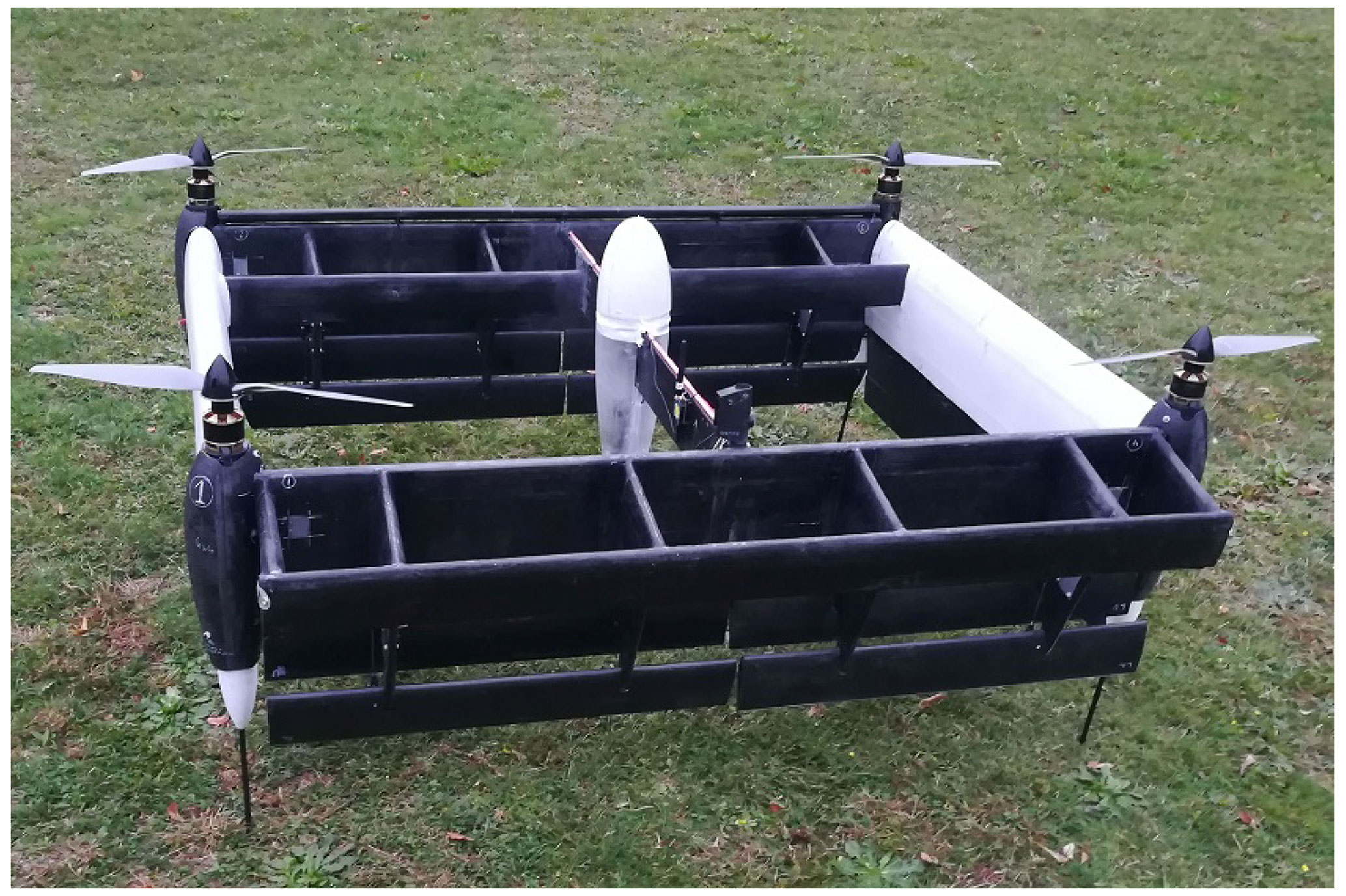
The goal of this paper is to investigate and optimise multi-element airfoils for application to AWE systems. The work aims to contribute to the existing knowledge base on the topic, which has been recently initiated. This is done by carrying out 2D steady-state computational fluid dynamics (CFD) simulations of a baseline multi-element airfoil in OpenFOAM for checking the simulation feasibility and then optimising the geometry by varying a range of geometrical parameters. The baseline simulations are shown in Sect. 2, and the optimisation is discussed in Sect. 3. The conclusions are drawn in Sect. 4. This work is carried out as part of a project with the Swiss company Skypull AG, who are developing a box-wing double-wing AWE system with multi-element airfoils as shown in Fig. 1. This real application introduces constraints related to the overall mass of the drone and its structural integrity, which have an influence on the aerodynamic design.

Figure 1 The drone of Skypull AG.

2 Baseline simulations

In this section, the details of the baseline geometry are presented, including the meshing and feasibility studies.

2.1 Geometry

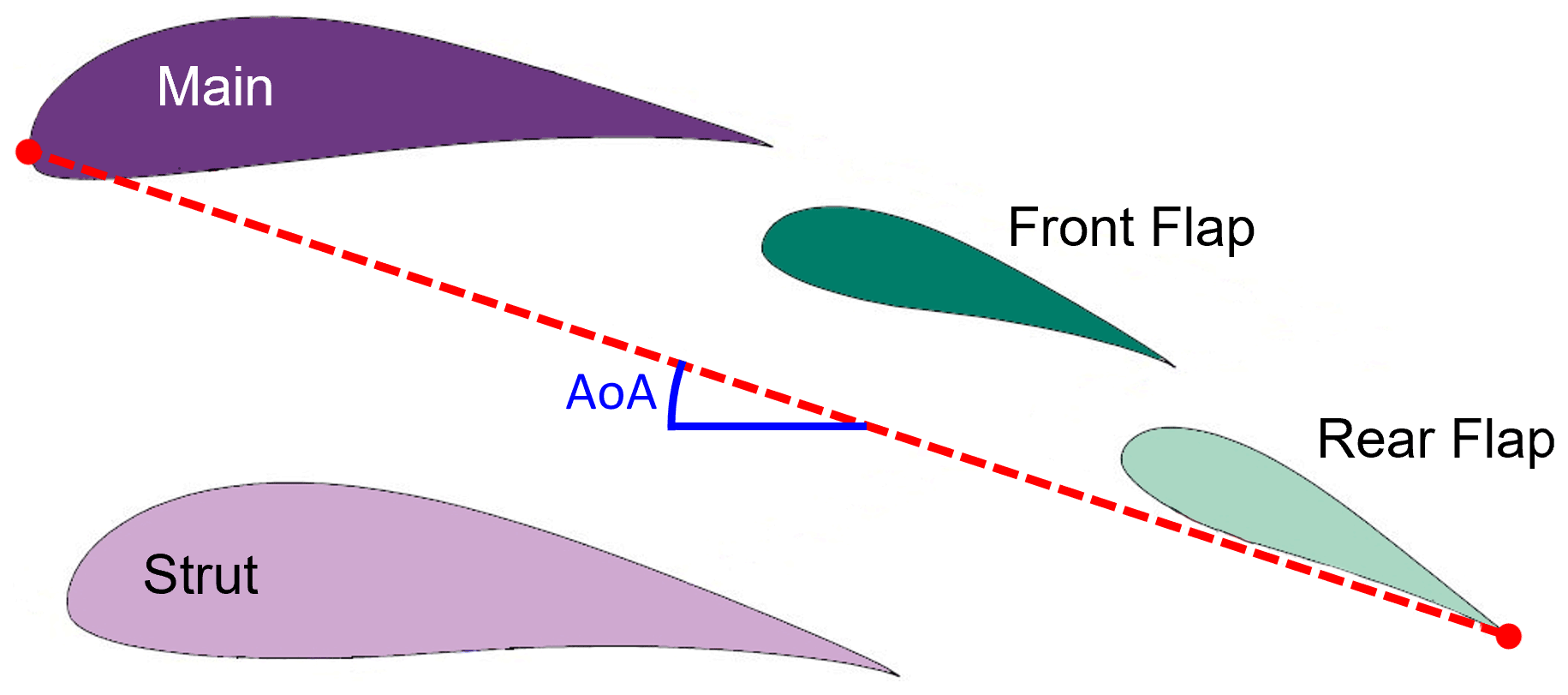
For the baseline simulations, an existing multi-element airfoil developed for conventional wind turbine applications called MFFS-018 was used (Ragheb and Selig, 2011). This airfoil was designed by converting the outer geometry of an existing wind turbine airfoil (DU 00-W-401) into several different multi-element airfoils using trial and error and estimating the resulting C_L and C_D using the multi-element airfoil analysis programme MSES (Ragheb and Selig, 2011; Drela, 2007). MSES supports the analysis and design of multi-element airfoils by solving the Euler equations with the finite-volume method. This allows a large range of different conditions to be captured, including predicting transitional separation bubbles and trailing-edge separation (Drela, 2007). The MFFS-018 airfoil demonstrated the highest C_L and was therefore chosen as the baseline in the present paper. The geometry was obtained for use in this work by manually scanning and digitalising the drawing of the airfoil in Ragheb and Selig (2011) to create a STEP file. The airfoil is divided into four sub-airfoils (or elements), called main, strut, front flap and rear flap as shown in Fig. 2. The dashed red line shows the overall chord, starting from the leading edge of the main airfoil and ending at the trailing edge of the rear flap. The definition of the angle of attack (AoA) used in the present work is also marked.

Figure 2 MFFS-018 multi-element airfoil baseline geometry (Ragheb and Selig, 2011).

2.2 Simulation set-up

In this work, the CFD code OpenFOAM (Version 6) was applied to the baseline multi-element airfoil, set up for steady-state 2D RANS (Reynolds-averaged Navier–Stokes) simulations. OpenFOAM was chosen due to its ability to capture separated flow with reasonable computational power. It is recognised that 3D effects may have an influence on the results due to skewed inflow conditions, interactions between the box-wing sections and effects of the airfoil mounting devices (see Fig. 1). This is the subject of ongoing work.

Figure 3 (a) CFD domain. (b) Refinement zone around the profile. (c) Refinement layers around the elements.

Figure 4 Influence of cell sizes on (a) C_L and (b) C_D at AoA = 17^∘.

The mesh was designed via a grid dependency study, which involved successfully decreasing the cell size until C_L and C_D were not affected by the mesh itself. As a reference length a chord length of 1 m as defined in Fig. 2 was used to calculate C_L and C_D. By iteratively refining a starting mesh and morphing the resulting split-hex mesh to the surface, the mesh approximates the surface. This allowed us to mesh the airfoil in an efficient and automated manner – required later for the parametric study. The results of the mesh dependency study are shown for an AoA of 17^∘ in Fig. 4, where it can be seen that reducing the initial cell size (the size of the cell that was not manipulated by the snappyHexMesh utility, which is located far away from the airfoil) of the domain increased C_L until it became constant below about 20 mm. As well as this, reducing the initial cell size decreased C_D until it became constant below 20 mm. Studies at other AoAs showed consistent results. Therefore, an initial cell size of 20 mm has been chosen as optimal in this work. The Reynolds number was chosen to be Re=10⁶ in order to reflect realistic conditions corresponding to a relative wind speed of 15 m s⁻¹ and chord length of 1 m. The Spalart–Allmaras turbulence model (Nordanger et al., 2015) was chosen because no significant differences between different turbulence models were found and the one-equation model is comparatively efficient. For this study, it was assumed that the boundary layer was fully turbulent over the entire airfoil due to the high Reynolds number applied. Future work could investigate lower-Reynolds-number effects such as boundary layer transition models similarly to the work from Folkersma et al. (2019), but this is a secondary priority. In the end, each separate airfoil was refined with five mesh layers within the boundary layer, resulting in a domain containing 50 000 cells with maximal dimensions 0.3 m by 0.3 m. In order to describe how velocity behaves from the near-wall region, the y-plus term was introduced. The set-up resulted in a y-plus value of 30 with nutUSpaldingWallFunction (García-Rodríguez and Chacón Velasco, 2020), which indicates that the wall region was resolved properly (Pas, 2016). The resulting mesh, shown in Fig. 3, consists of hexahedrons and was created by the snappyHexMesh utility.

2.3 Simulation verification

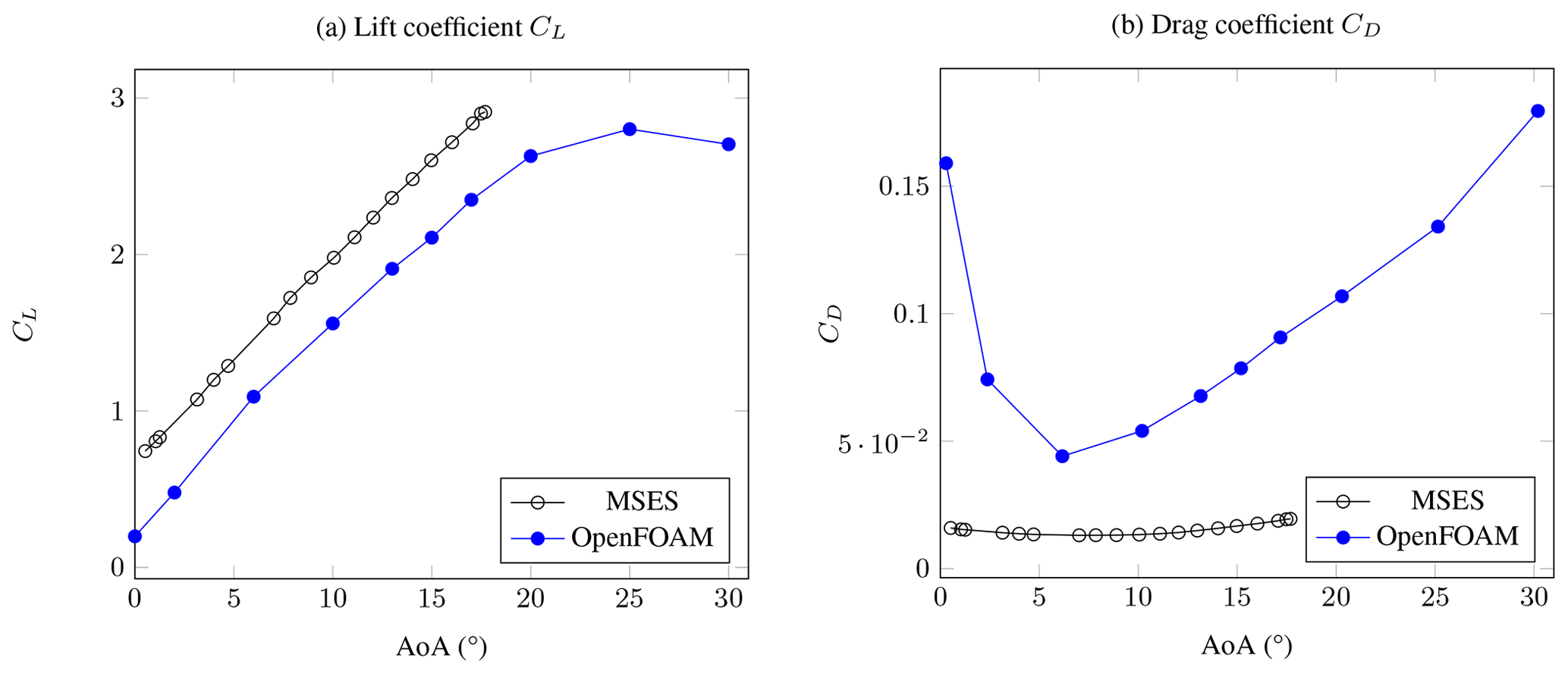
In order to verify the quality of the simulations in OpenFOAM, simulations for a range of AoAs were compared with MSES simulations from the original study as described in Sect. 2.1 above (Ragheb and Selig, 2011). A true validation could not be done because higher-fidelity simulations or wind tunnel measurements are not available to the authors' knowledge. The results are shown in Fig. 5. The C_L-vs.-AoA plot shows that the MSES and the OpenFOAM simulations match fairly well, except around the separation point, as expected, because the MSES results were obtained with natural transition, whereas the OpenFOAM simulations were carried out for a fully turbulent boundary layer. The small offset may be due to different definitions of the zero AoA, which was not clear in Ragheb and Selig (2011). The C_D-vs.-AoA plot shows that MSES under-predicts the drag compared to OpenFOAM quite significantly. This is also to be expected as CFD takes pressure drag due to flow separation into account (Vinh et al., 1995), whereas MSES does not. As well as this, the discrepancy could be due to the fact that the MSES results were obtained with natural transition, whereas the OpenFOAM simulations were carried out for a fully turbulent boundary layer. Even at low AoA values, some flow separation can be observed over multiple airfoils (as discussed later in Sect. 2.4). High-quality wind tunnel tests are required in order to fully assess the accuracy of both the CFD and the MSES simulations correctly. This is the topic of ongoing work. Thus, with the information available for this study, the set-up was therefore deemed suitable for further studies, although the absolute values of C_L and C_D should not yet be used directly for AWE designs.

Figure 5 Comparison of (a) C_L and (b) C_D with different AoAs between MSES and OpenFOAM.

2.4 Simulation results

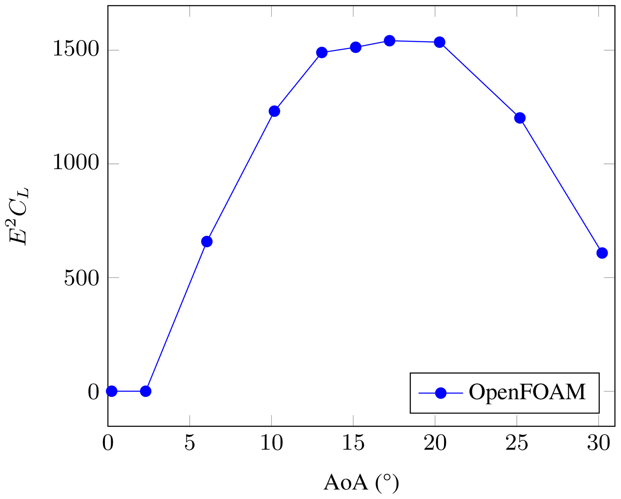
For this work, instead of C_L, the ratio E²C_L has been chosen as the optimisation parameter, where $E=C_{\mathrm{L}}/C_{\mathrm{D}}$, which is the glide ratio, and C_L and C_D are the total lift and drag coefficients of the drone. This variable was chosen since the power of an AWE system is proportional to $E_{\mathrm{eq}}^{\mathrm{2}}{C}_{\mathrm{L}}$ (Loyd, 1980), where C_L is the effective system lift coefficient and $E_{\mathrm{eq}}=C_{\mathrm{L}}/C_{{\mathrm{D}}_{\mathrm{eq}}}$ is the effective system glide ratio, including the drag of the tether (Bauer et al., 2018). In this work, however, the drag of the tether has not been yet included due to its expected small contribution to the overall drag; $E_{\mathrm{eq}}=C_{\mathrm{L}}/C_{\mathrm{D}}$ has been used, where C_L and C_D refer to the total lift and drag coefficients of the drone, respectively. Ongoing work involves comparing the results with and without tether drag.

The baseline OpenFOAM results in terms of E²C_L are shown in Fig. 6, calculated from the values of C_L and C_D from Fig. 5. It can be seen that the optimum E²C_L lies at AoA = 17^∘.

Figure 6 Performance of the baseline airfoil in terms of E²C_L vs. AoA simulated in OpenFOAM.

In order to examine the flow behaviour in more detail, plots of the pressure coefficient (C_p) vs. distance from the main leading edge in the overall chord direction along the airfoil and streamline visualisations are shown for AoA = 0^∘ in Fig. 7, for AoA = 6^∘ in Fig. 8, for AoA = 10^∘ in Fig. 9, for AoA = 17^∘ in Fig. 10 and for AoA = 25^∘ in Fig. 11. The C_p distribution has been calculated for each airfoil element using the local normal pressure force acting along the surface and the relative chord length of the individual elements, defined in Fig. 2. The total chord length is 1 m. The x axis represents the distance from the main leading edge in the main chord direction along the airfoil. The designation in the legend has been abbreviated for front flap and rear flap as F-Flap and R-Flap, respectively. Furthermore, the following C_p diagrams of the individual elements are subdivided into suction and pressure side, and this is also noted in the legend.

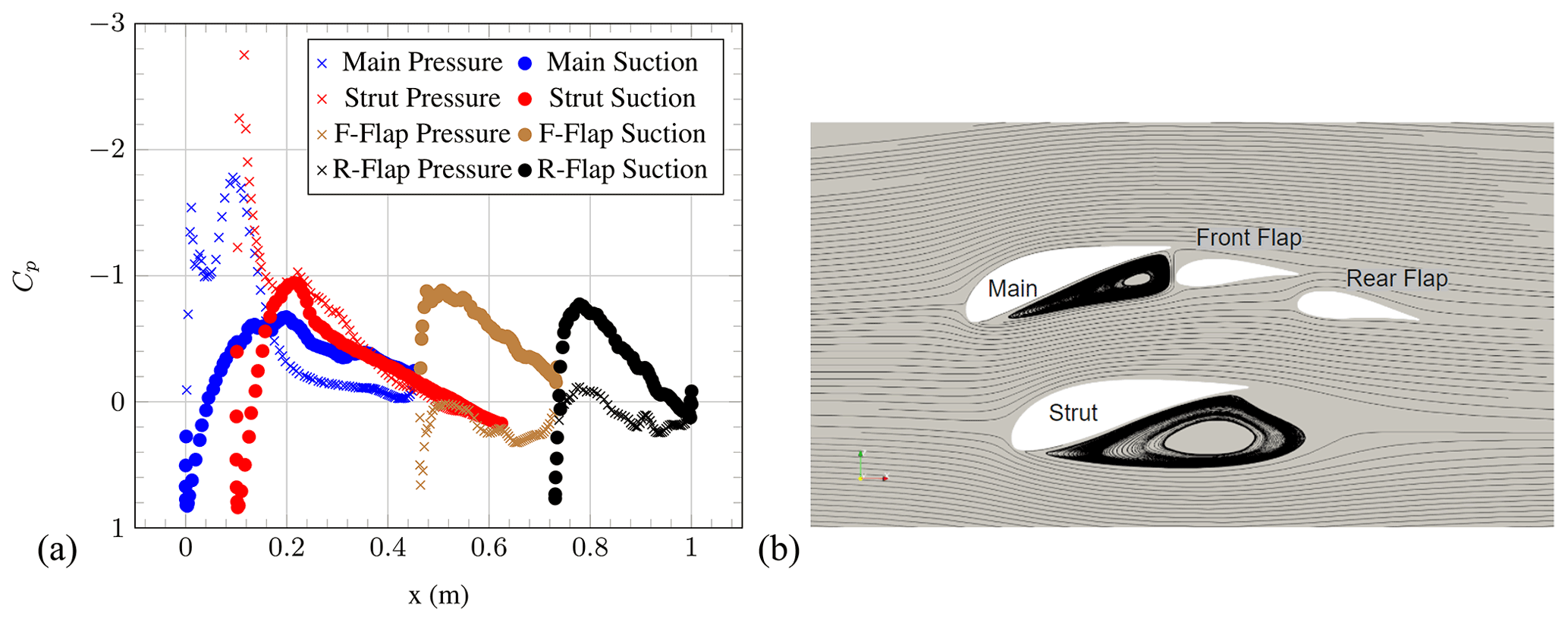
Figure 7 (a) Pressure coefficient of the individual element airfoils and (b) streamlines at AoA = 0^∘ (OpenFOAM simulations).

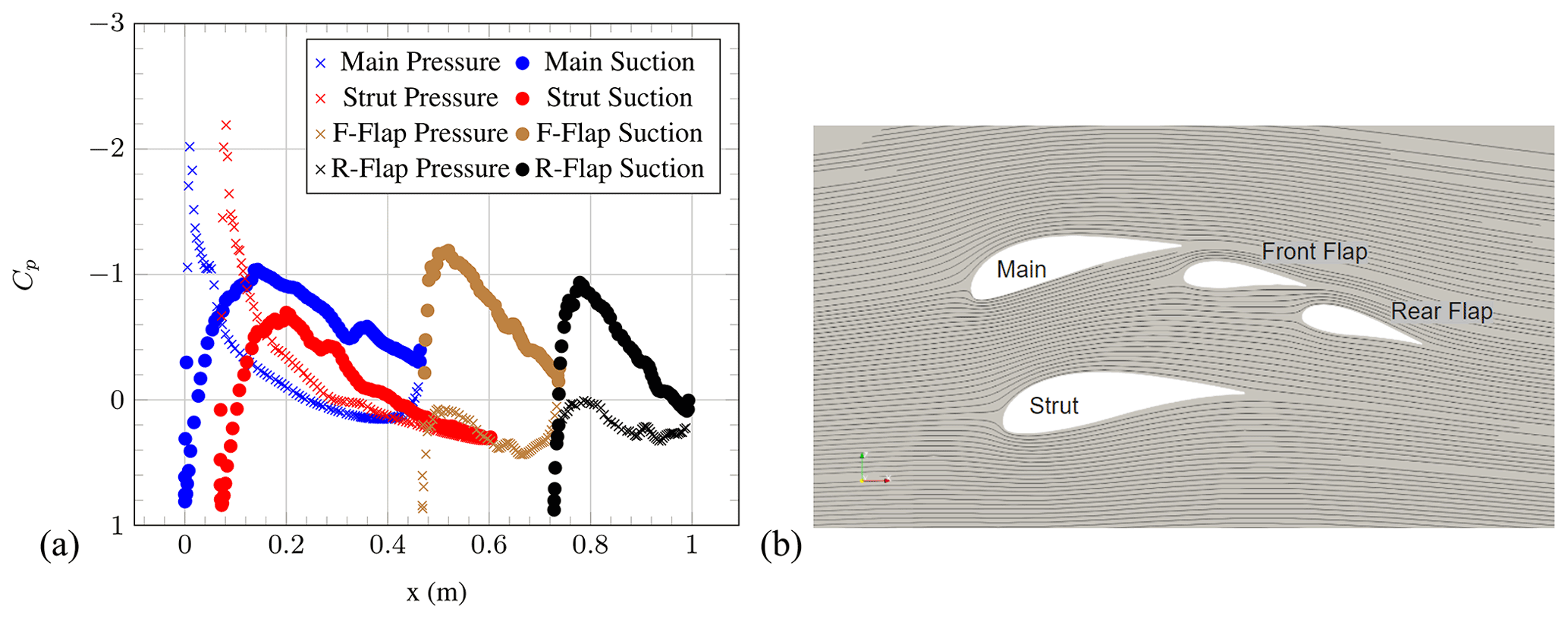
Figure 8 (a) Pressure coefficient of the individual element airfoils and (b) streamlines at AoA = 6^∘ (OpenFOAM simulations).

Figure 9 (a) Pressure coefficient of the individual element airfoils and (b) streamlines at AoA = 10^∘ (OpenFOAM simulations).

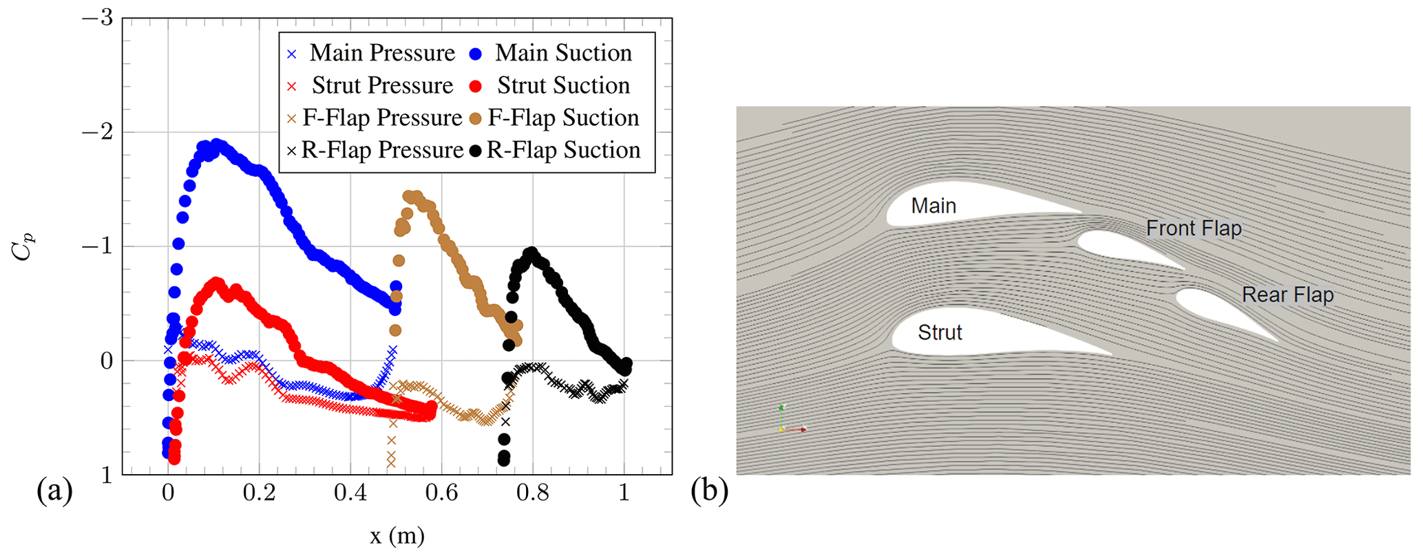
Figure 10 (a) Pressure coefficient of the individual element airfoils and (b) streamlines at AoA = 17^∘ (OpenFOAM simulations).

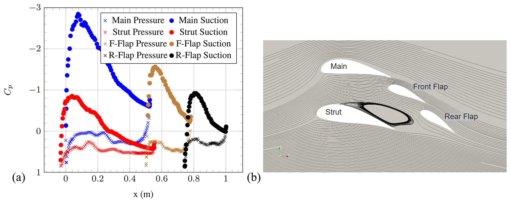
Figure 11 (a) Pressure coefficient of the individual element airfoils and (b) streamlines at AoA = 25^∘ (OpenFOAM simulations).

At AoA = 0^∘, a substantial pressure-side flow separation can be observed at the main and strut elements. The flow separation is caused by the (local) negative AoA of the main and strut elements, although the overall airfoil AoA is zero. Furthermore, a small counter-rotating re-circulation zone at the front of the front flap can be seen. The expected counter-rotating re-circulation zone behind the strut to match the opposing streamline direction cannot be observed on the streamline plot. Further investigations are under way. However, the C_p distributions of the front flap and rear flap seem to be mostly unaffected by flow separation. An increase in AoA to 6^∘ leads to a disappearance of the flow separation, although the C_p distributions for the main and strut elements still indicate small separated regions. Ongoing work is investigating the exact point at which this disappearance of flow separation takes place.

The same behaviour can be observed at AoA = 10^∘. At AoA = 17^∘, the C_p distribution indicates a lack of flow separation over all of the airfoil elements. As well as this, the airfoil configuration appears to generate the greatest area under the curves, agreeing with the fact that C_L is highest at this AoA. Suction-side flow separation for the strut element can be seen at AoA = 25^∘. This is visible in the streamline visualisation as well as in the C_p distribution plot. This leads to a decrease in C_p. In general, it is important to notice that this flow behaviour could be affected by both 3D effects and the Reynolds number. Possible 3D effects include slight sweep angles that may result from the drone's flight path offset from the oncoming wind, edge effects near to the corners of the box wind and effects of the airfoil mounting structures. The high Reynolds number chosen implies fully turbulent flow; however, if the relative wind speed were to reduce below the value at which laminar–turbulent transition is expected (on the order of 10⁵), the drag could increase significantly.

3 Airfoil parametric study

In this section the parametric study is carried out. For that, several parameters of the multi-element airfoil were changed and the impact on E²C_L quantified. The limits of these changes were set by the structural and manufacturing limits given by the designers.

3.1 Parametric study strategy

For the parametric study, the effects of certain geometry changes on the airfoil performance were first investigated for the optimal AoA of 17^∘. For this purpose, individual parameters were changed and simulated and the result in terms of C_L, C_D and E²C_L were compared with the baseline performance. The AoA was not chosen as an input variable in this study in order to reduce the number of simulations carried out, although it is recognised that this could lead to a local maximum being missed and is the topic of ongoing work.

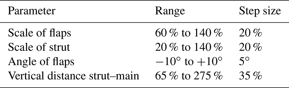
The parameters that were investigated are summarised in Table 1. The “relative scale” refers to the relative change in size of an individual airfoil element compared to the original geometry in both x and y directions equally; i.e. an increase in chord length increases the thickness equally to maintain the shape of the airfoil. A value of 100 % refers to no change compared to the baseline. The total chord length of the multi-element airfoil is maintained at all times, meaning that a relative increase in the size of one airfoil leads to a reduction in the size of the others. The “relative angle” refers to the rotation in degrees relative to the baseline angle, with an axis of rotation at the leading edge of the element in question. The “vertical distance of strut” refers to the relative distance between the centrelines of the strut and the main airfoils compared to the baseline of 100 %. When these parameters were changed, it was taken care that the “overhang” and “gap” between the main and the front flaps as well as between the two flaps remained the same (see Fig. 12). If an AoA variation were to be included in the future, the changes in these parameters due to changing AoA would have to be taken into account. The reference point was always the leading edge of the elements. The ranges and step sizes of the different configurations simulated in this work are also given in the table. The ranges were defined by the designers of the AWE system due to their structural and manufacturing constraints. These constraints were introduced by the drone designers, who carried out separate calculations in order to obtain the maximum allowable mass and thickness of the components. The parametric study matrix represents 576 discrete parametric combinations. Simulating all these combinations would have been beyond the scope of this work and will be part of following studies. For this reason, only the influences of the individual changes were assessed.

Table 1 Summary of varied parameters; 100 % refers to the baseline case.

Figure 12 Definition of overhang and gap.

Figure 13 Effect of relative scale of front and rear flap on (a) C_L, (b) C_D and (c) E²C_L.

For each simulation, the airfoil and mesh were re-created manually in OpenFOAM. Automated optimisation algorithms such as the gradient descent method (Ruder, 2016; Zhang et al., 2021) and the efficient global optimisation (EGO) algorithm (Jones et al., 1998) were considered, but the manual method was used for this initial study because this approach has the potential to help us understand the aerodynamics of multi-element airfoils for this application better. Automated optimisation procedures could be applied in the future, but it is preferable to first have a detailed understanding of the problem. Ongoing work involves the application and testing of various optimisation algorithms. However, this does mean that the optimum may have been missed because not all combinations of all parameters were studied.

3.2 Parametric study results

Each geometry modification was found to have a different impact on the performance, as discussed in the following sections.

3.2.1 Relative scale of flaps

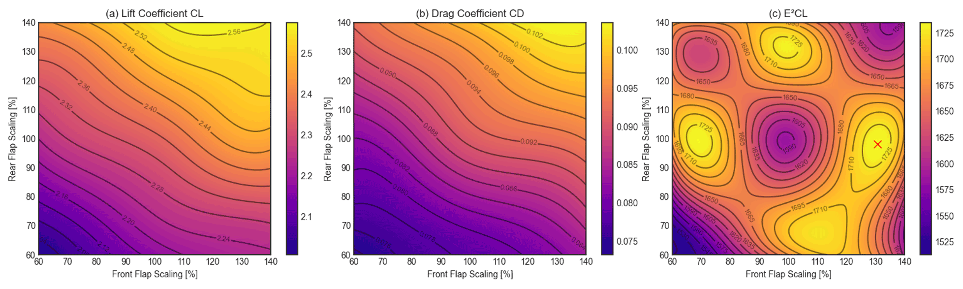
Figure 13 shows how the relative scales of the rear and front flaps influence the aerodynamic performance of the airfoil. For each plot, the relative scale of the front flap is shown on the x axis and the relative scale of the rear flap on the y axis. The colours refer to the absolute values of C_L, C_D and E²C_L. A cubic interpolation between the simulated points spaced every 0.1 % is carried out using the Python package “scipy.interpolate”. It can be seen that larger relative scales of the front flap and rear flap result in higher C_L and C_D values, leading to a non-linear variation in E²C_L with a maximum improvement of 7.7 % compared to the baseline, at a front-flap scaling factor of 131 % and a rear-flap scaling factor of 98 %. However, it should be noted that the effect of the front-flap scaling is quite symmetrical – reducing the scale by 30 % has a similar positive influence on the results to increasing it by 30 %. In this case, the manufacturer chose the larger value to ease manufacturing, but the lower value should be checked in the future. In Fig. 18 at the end of this section a comparison between the baseline geometry (a) and the geometry with the optimal front-flap scale (b) is shown.

Figure 14 Effect of relative strut scale on (a) C_L, (b) C_D and (c) E²C_L.

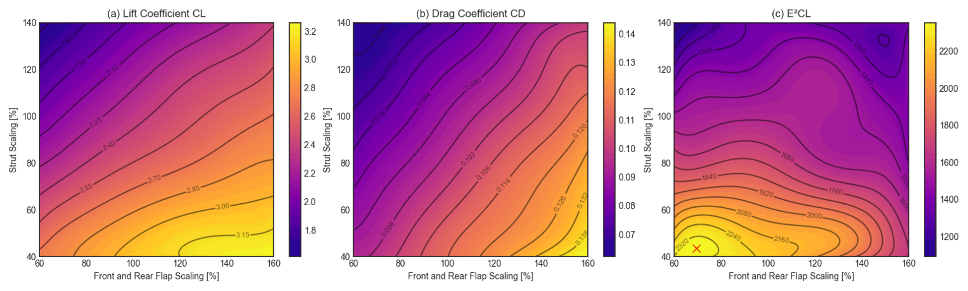
Figure 15 Effect of relative strut and flap scale altered together on (a) C_L, (b) C_D and (c) E²C_L.

3.2.2 Relative scale of strut

As shown in Fig. 14, a different effect can be seen when varying the relative scale of the strut element. Reducing the relative scale of the strut element leads to higher C_L and only a slightly higher C_D. The reason for this is that the flow around the strut disturbs the flow around the main profile less if it is relatively small. This leads to the fact that E²C_L can only be improved by decreasing or neglecting the relative scale of the strut element. Extrapolating this result leads to the conclusion that the strut element is not beneficial in this aerodynamic system and should be removed unless required for structural reasons. Within the range varied in this study, the smallest relative scale of 20 % resulted in an improvement in E²C_L of 39.9 %. In Fig. 18 at the end of this section a comparison between the baseline geometry (a) and the geometry with the optimal strut scale (c) can be seen. Although it is not thought to affect the conclusions of this work, note that the behaviour of the interpolations at the turning points of the graphs in Fig. 14 could be improved in the future with alternative, shape-preserving optimisation techniques.

3.2.3 Combined scaling of flaps and strut

In order to consider the aerodynamic interactions between the flaps and the strut element, the strut, front-flap and rear-flap scales were varied together. For that, the front and rear flaps were always scaled equally. The results in Fig. 15 show a clear interaction between the flap and strut scales. In order to achieve the same C_L, a smaller strut was required for small flaps, while a larger strut was needed for larger flaps. The same applied to C_D but in a different ratio. Therefore, it was not advantageous to make the flaps larger than 120 % or the strut larger than 60 % because above this size the optimal range could no longer be achieved. A maximum improvement in E²C_L of 46.6 % at a strut scaling of 43 % and a flap scaling of 69 % could be reached. Due to the mesh inaccuracies, a slight discrepancy occurs between the optimum value of this combination and the sum of the separate optimum values of strut and flaps. Furthermore, it must be noted that in the combined variant both flaps were simulated with the same scaling. The reason for this is the simplified presentation of the results and the greater impact on the understanding of the geometry changes.

3.2.4 Relative angles of flaps

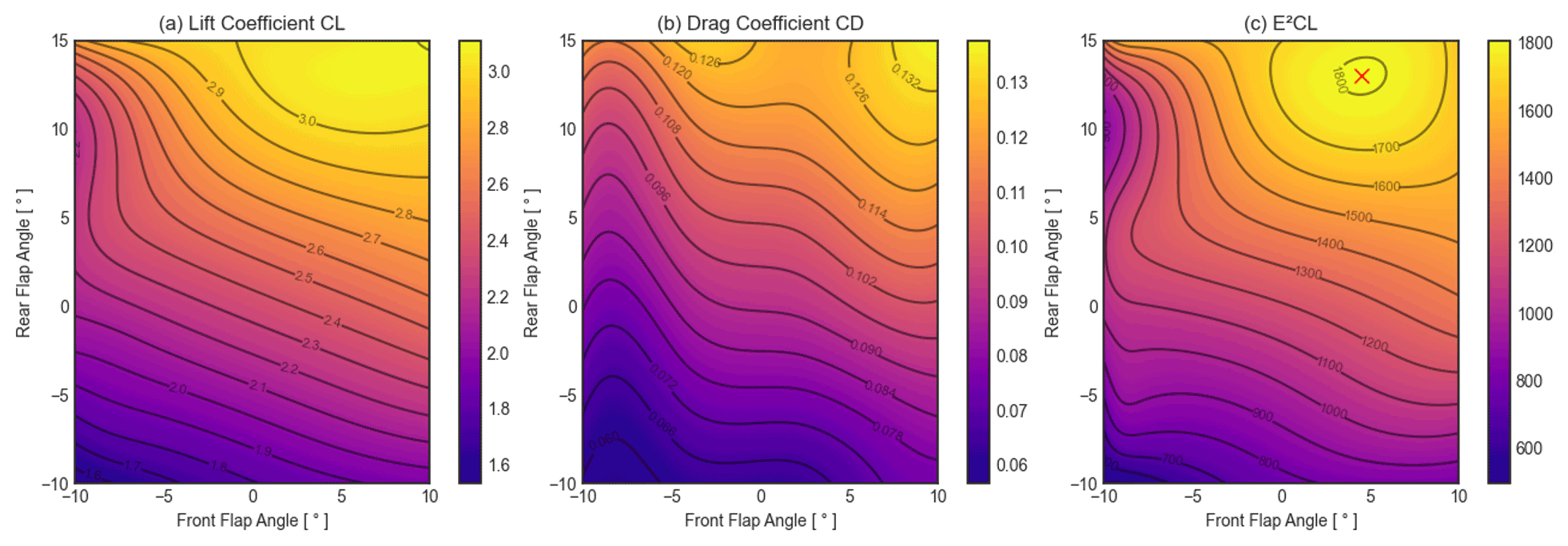
In a further step, the relative angle of the front flap and rear flap was studied. For that, the relative angles of both flaps were varied independently, as shown in Fig. 16. The result shows that the front flap has to be adjusted less steeply than the rear flap in order to improve E²C_L by 11.9 %. This gives the airfoil a more streamlined overall shape, which helps to deflect the flow in stages and avoid flow separation. In Fig. 18, a comparison between the baseline geometry (a) and the geometry with a rotated rear flap (d) is shown.

Figure 16 Effect of relative flap angles on (a) C_L, (b) C_D and (c) E²C_L.

Figure 17 Effect of strut's vertical distance on (a) C_L, (b) C_D and (c) E²C_L.

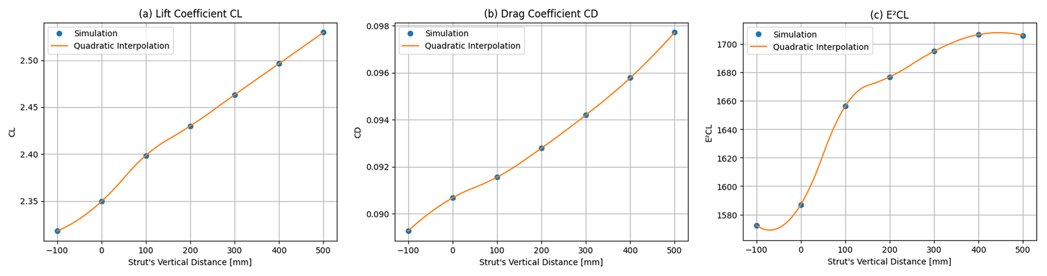
3.2.5 Relative vertical distance of strut

The last optimisation is the modification of the vertical distance of the strut element relative to the main element. The results in Fig. 17 show that it is most beneficial to increase the distance between the main and strut elements, meaning shifting the strut element further down. This result shows once again that the strut element is aerodynamically not beneficial since it disturbs the flow around the main airfoil. It can be seen that the E²C_L value stagnates at higher vertical distances, meaning that no further increase can be achieved by moving it further away. This makes sense since the strut element at some point is not part of the aerodynamic system and airfoil anymore and does not disturb the flow. The maximum possible improvement in E²C_L is only 7.5 %. In Fig. 18, a comparison between the baseline geometry (a) and the geometry with a greater distance between strut element and main airfoil (e) is visible.

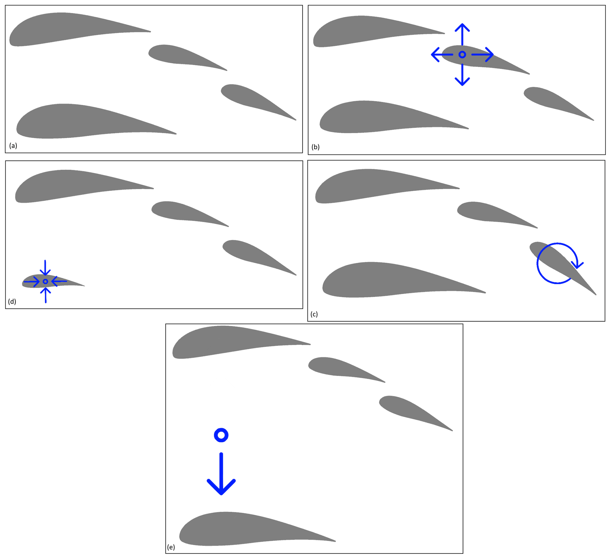
Figure 18 (a) Original geometry; (b) example of geometry with greater front-flap scale (140 %); (c) example of geometry with steeper rear-flap angle (−10^∘); (d) example of geometry with smaller strut scale (40 %); (e) example of geometry with greater distance between main element and strut (275 %).

3.3 Optimal choice of geometry

The results above have shown that the optimal geometry for maximising E²C_L within the given manufacturing and structural constraints and within the constraints of this parametric study has the following properties compared to the baseline:

• The relative scale of the front flap is 131 %.

• The relative scale of the rear flap is 98 %.

• The relative scale of the strut is 20 %.

• The relative angle of the front flap is 5^∘.

• The relative angle of the rear flap is 13^∘.

• The relative vertical distance of the strut is 500 mm.

The resulting geometry could increase the E²C_L by 50 % in total compared to the baseline geometry. The aerodynamics of the baseline and the optimal geometry can be compared by examining the wake region, as shown in Fig. 19. For that, four different slices in the wake region were chosen: Position 1 refers to a distance of 5 % of the chord length (0.05c) downstream of the trailing edge of the rear flap, Position 2 to 0.1c, Position 3 to 0.15c and Position 4 to 0.2c. The example in Fig. 19 shows a wake analysis with a distance of 0.2c after the trailing edge. The white line represents the y axis of the following Fig. 20, and 0 means the beginning and 1 the end of the y axis, respectively.

Figure 19 An example of the position of one of the vertical lines through the wake.

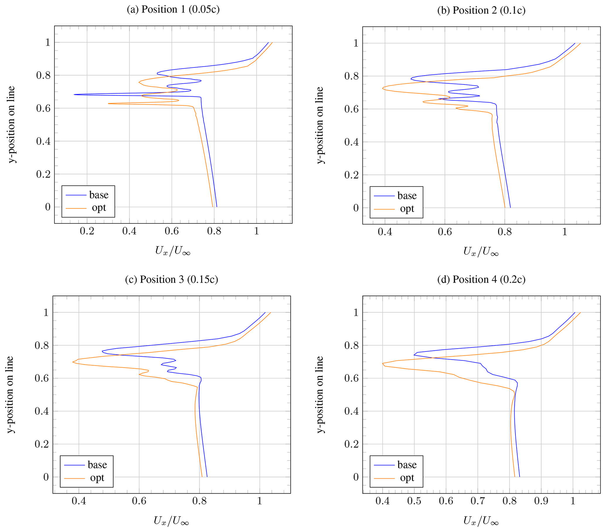
Figure 20 Velocity profile in wake region at (a) Position 1 (0.05c), (b) Position 2 (0.1c), (c) Position 3 (0.15c) and (d) Position 4 (0.2c).

Figure 20 shows the velocity profiles along a vertical line through the wake at these four positions for the baseline (blue) and optimal (orange) geometries. It can be seen that the wake of the baseline geometry has a much lower minimum velocity directly downstream of the trailing edge of the rear flap (Position 1). At Positions 2–4, however, the velocity profile of the optimised geometry forms a smooth U-shaped profile more quickly, whereas the baseline geometry still contains the wakes of the separate elements. This indicates that the overall drag is higher. This agrees with previous work – according to Pomeroy (2016), the type of wind speed profile seen here for the optimised geometry indicates better wake properties. However, it should be noted that even more improvements could be obtained with an optimisation process that does not miss out any combination of geometries.

3.4 Suitability of multi-element airfoils for AWE systems

Previous work indicated that the performance (in terms of E²C_L) of AWE systems with multi-element wings can be increased by up to 720 % compared to AWE systems with conventional wings (Ragheb and Selig, 2011). The present work used CFD and showed that this geometry could be improved aerodynamically within the structural and manufacturing constraints by 46.6 %, by altering the relative scaling and angles of the individual elements. Therefore our work supports the hypothesis that multi-element airfoils have high potential for application to AWE systems and shows that their performance can be enhanced even more by a parametric study.

However, the study was limited to 2D CFD and only involved manual variations. The consideration of 3D effects will increase the drag and therefore reduce the performance. However, more advanced optimisation methods could help identify some improved optimisation geometries. As well as this, inclusion of the tether drag in the optimisation process is expected to improve the results.

It should also be noted that despite the improved aerodynamic performance, these types of airfoil could pose some structural and manufacturing difficulties. This study did take into account the limitations of one company, but the details need to be examined further. For example, the distances between the individual profiles are limited because space is needed for production and otherwise there is no room for the tool. Future work could therefore involve taking into account the limitations connected with the use of manufacturing tools in the optimisation process in the future. Additionally, a coupled aerodynamic and structural solver would be beneficial, as well as 3D CFD simulations and accompanying wind tunnel tests.

4 Conclusions

In this study, the application of multi-element airfoils to AWE systems was investigated. This was done by carrying out 2D steady-state computational fluid dynamics simulations of an existing multi-element airfoil from the literature in OpenFOAM and then optimising the geometry by varying various geometrical parameters until the best improvements in performance were found. In order to quantify and improve the airfoil performance, the term E²C_L was used, where E is the glide ratio and C_L is the lift coefficient of the drone.

An existing multi-element airfoil designed for conventional wind turbines was used as the baseline. Following a grid dependency study, baseline simulations were compared to existing simulations using the software MSES, an Euler solver. Although the lack of wind tunnel data or higher-fidelity simulations did not allow a formal validation to be carried out, this comparison did confirm the feasibility of the simulations.

For the parametric study, the optimum angle of attack for the baseline geometry was first identified as 17^∘. Next, several geometrical features including the relative scale and angle of the individual airfoil elements were varied separately and in combination in order to identify the optimal configuration. The constraints were given by manufacturing and structural limits of the AWE system designer. This showed that significant improvements of up to 46.6 % in E²C_L are possible. Further optimisations would be possible using automatic optimisation algorithms rather than adjusting the geometry manually. Additionally, an optimisation strategy that took into account the structural properties and the manufacturing limitations would be beneficial in the future. Further investigations into 3D effects and tether–drone interactions are ongoing.