the Creative Commons Attribution 4.0 License.
the Creative Commons Attribution 4.0 License.
 | 08 Sep 2022
FarmConners wind farm flow control benchmark – Part 1: Blind test results
Filippo Campagnolo
Thomas Duc
Irene Eguinoa
Søren Juhl Andersen
Vlaho Petrović
Lejla Imširović
Robert Braunbehrens
Jaime Liew
Mads Baungaard
Maarten Paul van der Laan
Guowei Qian
Maria Aparicio-Sanchez
Rubén González-Lope
Vinit V. Dighe
Marcus Becker
Maarten J. van den Broek
Jan-Willem van Wingerden
Adam Stock
Matthew Cole
Renzo Ruisi
Ervin Bossanyi
Niklas Requate
Simon Strnad
Jonas Schmidt
Lukas Vollmer
Ishaan Sood
Johan Meyers
Wind farm flow control (WFFC) is a topic of interest at several research institutes and industry and certification agencies worldwide. For reliable performance assessment of the technology, the efficiency and the capability of the models applied to WFFC should be carefully evaluated. To address that, the FarmConners consortium has launched a common benchmark for code comparison under controlled operation to demonstrate its potential benefits, such as increased power production. The benchmark builds on available data sets from previous field campaigns, wind tunnel experiments, and high-fidelity simulations. Within that database, four blind tests are defined and 13 participants in total have submitted results for the analysis of single and multiple wakes under WFFC. Here, we present Part I of the FarmConners benchmark results, focusing on the blind tests with large-scale rotors. The observations and/or the model outcomes are evaluated via direct power comparisons at the upstream and downstream turbine(s), as well as the power gain at the wind farm level under wake steering control strategy. Additionally, wake loss reduction is also analysed to support the power performance comparison, where relevant. The majority of the participating models show good agreement with the observations or the reference high-fidelity simulations, especially for lower degrees of upstream misalignment and narrow wake sector. However, the benchmark clearly highlights the importance of the calibration procedure for control-oriented models. The potential effects of limited controlled operation data in calibration are particularly visible via frequent model mismatch for highly deflected wakes, as well as the power loss at the controlled turbine(s). In addition to the flow modelling, the sensitivity of the predicted WFFC benefits to the turbine representation and the implementation of the controller is also underlined. The FarmConners benchmark is the first of its kind to bring a wide variety of data sets, control settings, and model complexities for the (initial) assessment of farm flow control benefits. It forms an important basis for more detailed benchmarks in the future with extended control objectives to assess the true value of WFFC.
- Article
(9855 KB) - Full-text XML
- BibTeX
- EndNote


Wind farm flow control (WFFC) promises to mitigate the losses due to aerodynamic turbine–turbine interactions and can potentially provide several benefits to reduce the cost of energy in the design and operation of wind farms. Its most prominent benefits are the potential increase in power production and/or alleviation of turbine structural loading at wind farms by reducing wake losses and encouraging energy entrainment into the farm. The phenomenon has been thoroughly investigated, with lower-order and high-fidelity flow and structural response models (e.g. Gebraad et al., 2016; Munters and Meyers, 2018; Duc et al., 2019; Hulsman et al., 2020), wind tunnel tests (e.g. Rockel et al., 2017; Bastankhah and Porté-Agel, 2019; Campagnolo et al., 2020; Bottasso and Campagnolo, 2021), and field experiments (e.g. Fleming et al., 2017; Annoni et al., 2018; Doekemeijer et al., 2021; Bossanyi and Ruisi, 2021; Simley et al., 2021). A comprehensive review of the power maximization through WFFC is presented in Kheirabadi and Nagamune (2019) and Andersson et al. (2021). To realize those benefits, the control strategy might be
-
axial induction control, in which some upstream turbines will lower their energy capture (also referred to as curtailment, down-regulation, or derating), hence increasing the wind velocity and reducing the turbulence downstream;
-
wake steering, in which some of the turbines will be misaligned to redirect the wake away from the other turbines, hence mitigating the wake effects; and
-
wake mixing where upstream turbines are dynamically up-regulated and down-regulated on short timescales to induce additional wake mixing and wake recovery, minimizing the losses further downstream.
A number of control-oriented models with different levels of complexity have been proposed in literature to implement those control strategies, but uncertainty remains high and a systematic validation and comparison under different control settings have been lacking. Validation and industrial implementation, in fact, is identified as one of the four key challenges within the WFFC field and thoroughly discussed in Meyers et al. (2022), where an in-depth review of the relevant studies is also presented.
In order to assess the performance of the WFFC technology, the capabilities of WFFC models should be evaluated. Accordingly, the FarmConners consortium (FarmConners, 2019) has launched a common benchmark for code comparison, where high-fidelity simulation results, wind tunnel experiments, and field data measured at a full-scale wind farm are brought together. This unique database combines the efforts of the connected WFFC projects of different sizes all over Europe and consists of four blind tests in total: (1) SMARTEOLE Sole du Moulin Vieux (SMV) field measurement campaign (Duc et al., 2019), (2) CL-Windcon wind tunnel experiments (CL-Windcon, 2016), (3) CL-Windcon large-eddy simulations (LESs) (CL-Windcon, 2016), and (4) TotalControl LES (TotalControl, 2018). Every data set is divided into a “calibration” and a “blind test” period to resemble field application of WFFC models. The calibration period involves both input and output features which can be used to calibrate the participating models under normal operation and limited control set points. In the blind test period, the calibrated models are to be run “blindly”, where only the input features are provided and their outputs are compared against the validation data set or the blind test reference, as well as each other.
Promoting data sharing and standardization for validation processes as well, one of the most relevant exercises with similar structure is Wakebench (Rodrigo et al., 2014; Moriarty et al., 2014), focusing on wind farm flow modelling under normal operation. Although sharing similar goals, the FarmConners benchmark blind tests conduct the performance evaluation exclusively under controlled operation. Therefore, the two benchmarks diverge in terms of test cases, quantities of interests and the validation metrics. However, the lessons learned from the extensive Wakebench experience (Doubrawa et al., 2020) is attentively taken into consideration while preparing the framework, aiming to extend the standard verification and validation (V&V) practices to include WFFC in wake research, globally.
The FarmConners benchmark is launched in TORQUE 2020 (Göçmen et al., 2020a), and in the end, 13 participants have submitted the results from their models, taking part in different blind tests. The overview of participants among the benchmark blind tests is presented in Table 1, and it should be noted that some participants have provided results from several models. The primary quantities of interest used in the model evaluations are the direct power comparisons at upstream and downstream turbines, as well as the power gain at the wind farm level by applying wake steering control strategy. Additional analysis on the wake loss reduction has also been presented to support the evaluation of the power performance, where relevant. It should be noted that the potential of the structural load alleviation, which was originally a quantity of interest in the benchmark, has been excluded from this study. This is due not only to the limited number of participating models capable of providing the necessary channels, but also to keep the focus on the most important benefit of the WFFC technology, as reported in the expert elicitation survey (van Wingerden et al., 2020). Similarly, scenarios with axial induction control that were included in the majority of the blind tests originally are also omitted due to limited participating model results. All the data collected for the benchmark can potentially be made available upon request for researchers; see Data availability section for details. The notebooks, including data snippets, where the blind test results are produced are also publicly available; see Code availability section for details.
Table 1Overview of the FarmConners benchmark participants (participant IDs P3–P20) per test case, per blind test. WFFC-oriented model comparison is performed separately for each column. The participants are colour coded for easy access through the article, where CL-Windcon wind tunnel experiments blind test results are discussed in Part 2 of the series.

The analysis and discussion of the results of the benchmark are divided into two parts. Here in Part I, the modelling of the large-scale rotors (blind tests 1, 3, and 4) is investigated, and in Part 2 the blind test results of the wind tunnel experiments are presented. Accordingly, Sect. 2 describes the SMV field campaign and presents the participating model results for single- and multiple-wake scenarios under upstream wake steering. High-fidelity simulations being a key enabler for the industrial implementation of WFFC, the subset of the extensive CL-Windcon LES database used for the FarmConners benchmark is detailed in Sect. 3. The participating models for the CL-Windcon LES blind tests are then evaluated for three and nine-turbine wind farm configurations, with 5- and 7-diameter (D) spacing respectively. Similarly, Sect. 4 utilizes up to eight-turbine subsets of a 32-turbine layout of a reference wind farm developed under the TotalControl project and compares the participating model results with the reference LES database under upstream wake steering.
Here in this article, we present the results from the large-scale rotor analysis of the FarmConners benchmark. The analysis is broken down into blind-test-specific, relatively stand-alone sections with limited cross-references and can be read separately if preferred.
The wind farm field data come from the Sole du Moulin Vieux (SMV) wind farm, located in the northern part of France (approximately midway between Paris and Lille) and operated by ENGIE Green. It consists of seven Senvion MM82 wind turbines (diameter of 82 m, nominal power of 2050 kW, hub height of 80 m; see Duc et al. (2019) for power and thrust coefficient, CT curves), organized in an irregular single row layout and labelled SMV1 to SMV7 from north to south. This wind farm has been used for the field tests of the French national project SMARTEOLE, whose results have been presented in Ahmad et al. (2017) and Duc et al. (2019) for field campaign 1 and in Simley et al. (2021) for field campaign 3. The layout of the wind farm is shown in Fig. 1, and the long-term wind rose observed at the site is presented in Fig. 2.
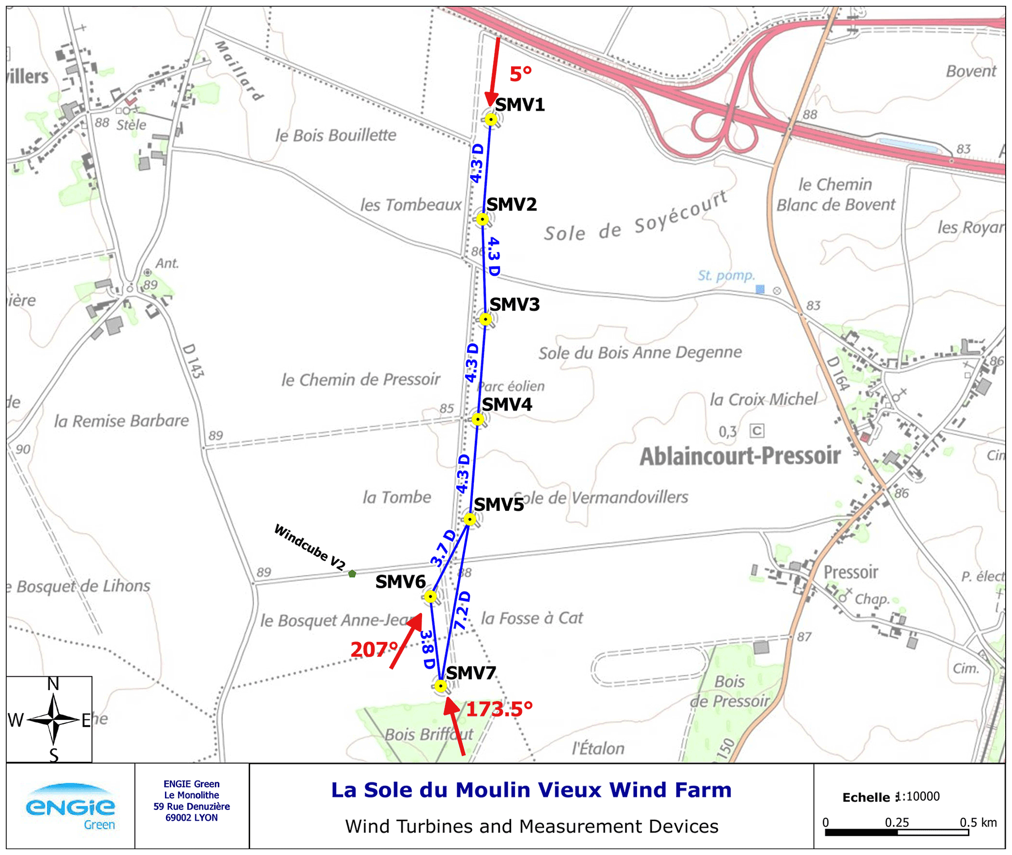
Figure 1Layout of SMV wind farm. Distances between wind turbines (normalized by their rotor diameter D = 82 m) and directions related to SMV6 and SMV5 are also shown. The location of the Windcube v2 sensor used for field campaign 2 is also indicated.

Figure 2Long-term wind rose for the SMV wind plant at hub height (80 m). It was obtained through a correlation process between short-term met-mast measurements on-site and long-term reference wind data (ERA5 reanalysis data). Taken from Simley et al. (2021).
The data set used for this benchmark exercise corresponds to the experiments carried out during field campaign 2, between May 2017 and March 2018. A ground-based lidar Windcube v2 was installed specifically for these field tests; its location close to SMV6 is displayed in Fig. 1.
Between 12 August 2017 and 3 October 2017, the SMV6 wind turbine was constantly misaligned for all wind directions. The averaged value of the turbine yaw offset during this 7-week period was −13.3∘ (turbine rotated anticlockwise when viewed from above), as illustrated in Fig. 11 below. This misalignment creates a wake steering that affects the downstream turbines, mostly SMV5 for wind directions between 200 and 215∘ and more slightly SMV4 to SMV1 for wind directions below 200∘.
2.1 Calibration and blind test data sets
A total of 12 months of normal operation data, from 1 October 2016 to 30 November 2017 (removing the 2 months for which the wake steering tests were conducted) were provided to the benchmark participants to help them calibrate their wake models. The calibration data consist of 10 min statistics (average, minimum, maximum, and standard deviation) of 10 of the most important variables of supervisory control and data acquisition (SCADA) data, including active power, wind speed and direction, yaw angle, pitch angle, outdoor temperature, and rotor and generator speed.
The data were filtered to keep only timestamps when all wind turbines were operating at the same time. Any timestamps when curtailments were detected in one of the turbines were also removed from the data set. Yaw angle and direction data were corrected for north alignment issues, making sure those signals were consistent over the full period. One turbine experienced a modification of its blade aerodynamic properties during the period. The effect of this change on turbine performance or anemometer wind speed measurement is unknown and could not be corrected.
The available data set for the wake steering experiment was unfortunately limited and could not be split into calibration and blind test subsets. Consequently the participants could only calibrate their wake deficit and superposition models and did not have any data to adjust either the parameters of their wake deflection models or the yaw loss function of the misaligned turbine.
The blind data set was prepared using the same procedure as for the calibration data set. The only difference is that the active power signal was removed for all turbines, and the wind speed signal was removed for all but the upstream turbines (SMV6 for south, south-westerly and SMV1 for northerly directions, indicated in Table 2). The Windcube data provided to the participants cover the full wake steering period and part of the calibration data, starting on 31 May 2017 and ending on 23 January 2018. All heights of measurements, ranging from 40 to 200 m, were kept in the data set. The participants were left free to use these data to calibrate any onsite atmospheric parameters, such as the turbulence intensity or the wind shear.
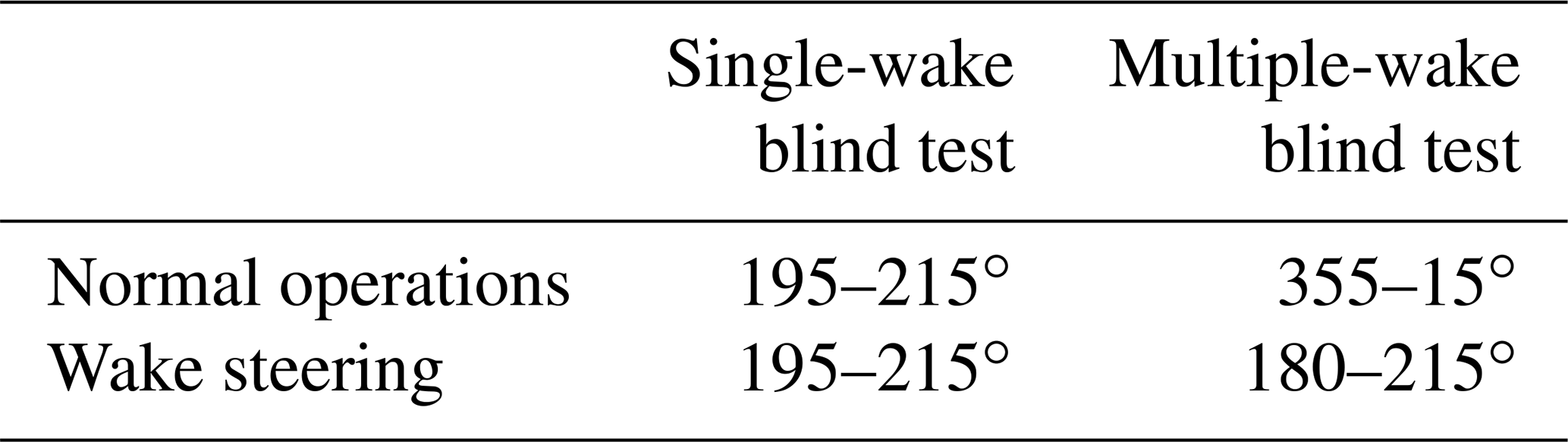
Table 2Summary of wind direction ranges for each of the blind tests.
2.2 Participating models
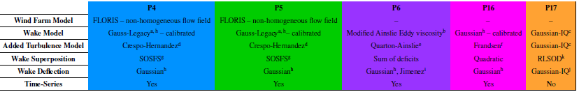
Within the FarmConners benchmark, in total five participants (IDs = P4, P5, P6, P16, P17) have taken part in the SMV wind farm field data blind test. The participating models cover a relatively broad range of assumptions, approximations, and parameters representing the flow behind a steered turbine. Here in this section, these participating models are briefly described, and implemented parameters are listed when relevant. Table 3 summarizes the prominent characteristics of the participating models. However, it should be noted that a seemingly identical model applied by the participants is likely to be calibrated differently, resulting in different performance in their predictions. This is further discussed in the detailed model descriptions per participant and highlighted in the blind test results later in the section.
Table 3Overview of the participating WFFC-oriented models, wind farm field data blind test. a Bastankhah and Porté-Agel (2014). b Ainslie (1988). c Ishihara and Qian (2018). d Crespo and Hernández (1996). e Quarton and Ainslie (1990) – with sum of difference. f Frandsen (2007) – IEC 2019 standard. g SOSFS – sum of squares free-stream superposition. h Bastankhah and Porté-Agel (2016). i Jiménez et al. (2010). j Qian and Ishihara (2018). k RLSOD – rotor-based linear sum of deficits.
2.2.1 P4
Wind speed and turbulence intensity. The wind speed was defined using nacelle anemometers at each wind turbine. The turbulence intensity was calculated using the mean and standard deviation of the anemometer data for each wind turbine.
Wind direction. It has been assumed that the average of the directions indicated by turbines' wind vanes was a good estimate of the free wind. The multiple-wake simulations used the average of all wind turbines measurements, and the single-wake simulations averaged SMV5 and SMV6 direction data.
Heterogeneous flow. The non-homogeneous flow field in the steady simulation was obtained through speed factors between turbines in free sectors (Vg – velocity factor, TIg – turbulence intensity factor). The factors were obtained using the wind turbine anemometer measurements, and they were applied regardless of the wind direction. These factors were defined with respect to the reference free wind turbine (SMV1 in multiple-wake case – Table 4 and SMV6 in single-wake case – Table 5).
Table 4P4: non-homogeneous factors for the multiple-wake case.
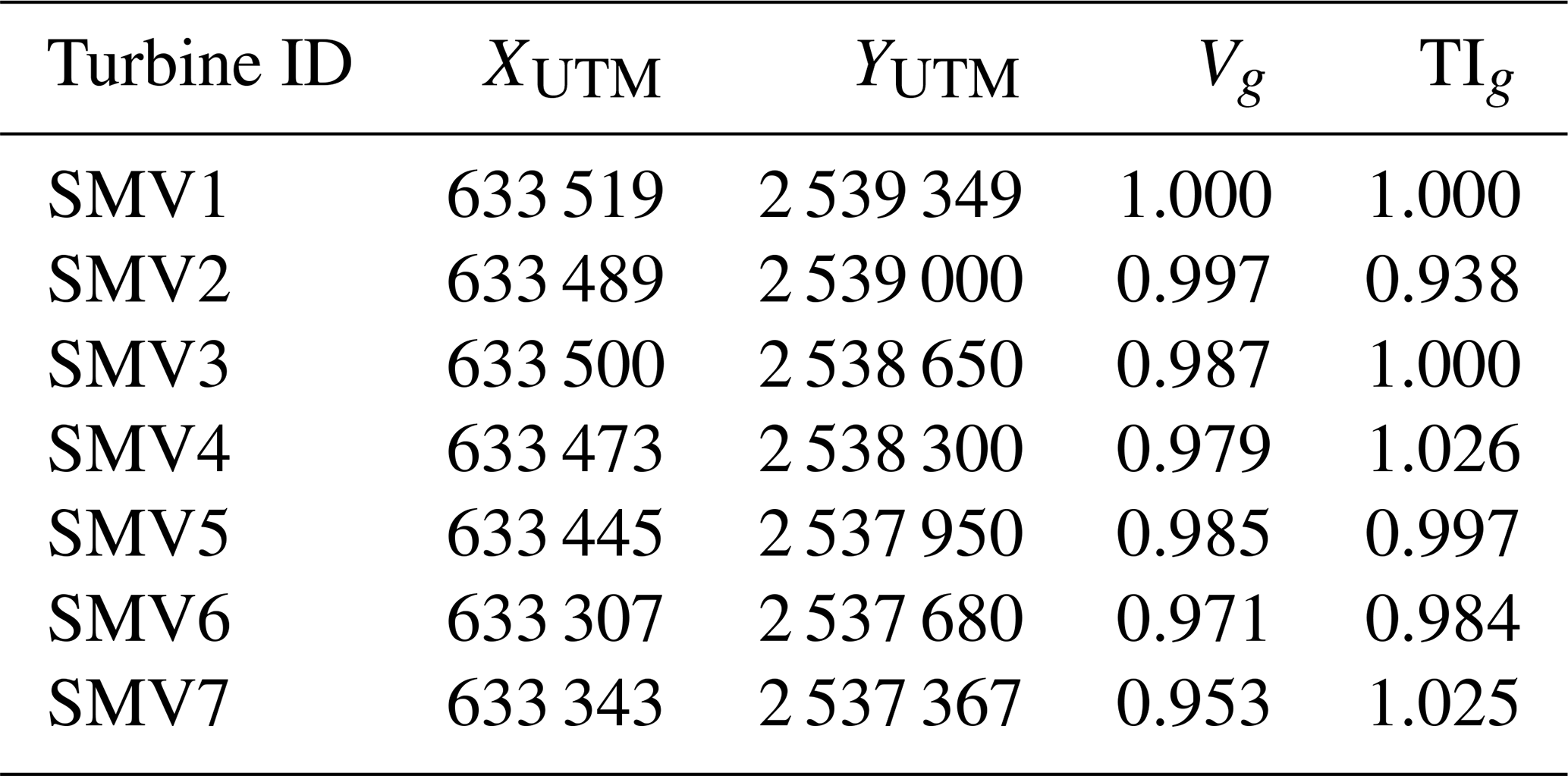
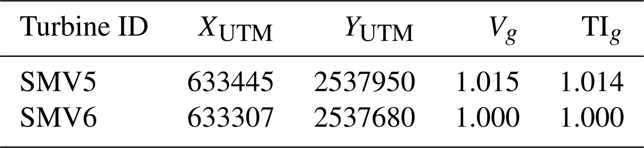
Free-stream wind speed and turbulence. The free-stream turbine conditions for the blind test simulations were determined by the free-stream turbines (SMV1 in multiple-wake case and SMV6 in single-wake case). For calibration, the free-stream wind speed and turbulence intensity were obtained averaging the free-stream turbines depending on the orientation. The heterogeneous factors were taken into account in order to refer the magnitudes to SMV1 (reference wind turbine for the multiple wake).
Wake model. The calibration performed by P4 was based on the FLORIS model, using the Gaussian velocity deficit model by Bastankhah and Porté-Agel (2014), and wake-added turbulence was modelled with the Crespo-Hernández model (Crespo and Hernández, 1996). The combination model selected was “SOSFS”, which uses sum of squares free-stream superposition to combine the wake velocity deficits to the base flow field (Katic et al., 1986). The yaw steering is represented by the deflection model Bastankhah and Porté-Agel (2016).
Calibration. The calibration process was performed using normal operation with multiple-wake data. The data were discretized with respect to the assumed wind direction (average of all wind turbines, bin size = 5∘) and free wind speed bins (bin size = 2 m s−1). From these data, a calibration matrix was created, by extracting mean values for velocity, turbulence intensity, and power in each wind turbine. Only cases where there is a wake effect were included in the calibration matrix. The calibration was performed using a genetic algorithm to obtain wake velocity and wake turbulence parameters. The parameters obtained in this process are presented in Table 6.
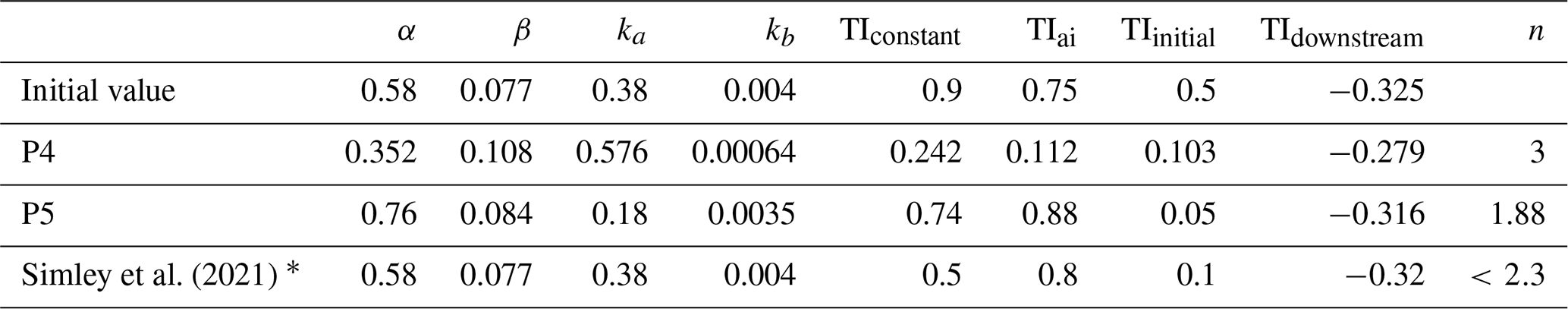
Simley et al. (2021)Table 6Calibrated parameters of the used velocity and turbulence sub-models of the relevant models used by participants P4 and P5, where α and β; ka and kb; and TIconstant, TIai, TIinitial, and TIdownstream are model parameters in FLORIS (NREL, 2021), and n is the yaw loss exponent in Eq. (1). * In Simley et al. (2021), the wake model fitting was realized by tuning the ambient turbulence intensity value rather than updating the model parameters. Within FLORIS (NREL, 2021), the Gauss velocity model (Bastankhah and Porté-Agel, 2014, 2016; Blondel and Cathelain, 2020; King et al., 2021) was used rather than the Gauss legacy model (Bastankhah and Porté-Agel, 2014, 2016) as for P4 and P5.
The comparison between the original experimental data, the average values used for calibration, and the simulation with the final calibrated parameters can be observed for specific wind conditions in Figs. 3 and 4, as illustrative examples. The original experimental data are shown as a boxplot, representing the median of the magnitudes and the dispersion of the data. The calibration values and the final simulation are represented by points for each wind turbine. Figure 3 presents the results for the bin centred in direction = 210∘ and wind speed = 10 m s−1, where the wake is evident for wind turbine SMV5 (single-wake sector). The agreement in the values in terms of velocity, turbulence intensity, and power is evident for wind turbine SMV5. Figure 4 presents results for the bin centred in direction = 185∘ and wind speed = 6 m s−1, where wind turbine SMV7 shows higher power and wind velocity than the rest of the turbines. The agreement in terms of velocity, turbulence intensity, and power is clear.

Figure 3P4: the y axes show (a) velocity (m s−1), (b) turbulence intensity (TI, –), and (c) power (P, kW). Comparison per SMV wind turbine (turbine numbering SMV1–SMV7 in x axis) between experimental data (boxplot), average values used for experimental calibration (ExpCalibration, blue circles), and simulation with calibrated parameters (P4, red circles). Bin direction = 210∘; bin wind speed = 10 m s−1. Empty black circles represent outliers.

Figure 4P4: the y axes show (a) velocity (m s−1), (b) turbulence intensity (TI, –), and (c) power (P, kW). Comparison per SMV wind turbine (turbine numbering SMV1–SMV7 on the x axis) between experimental data (boxplot), average values used for experimental calibration (ExpCalibration, blue circles), and simulation with calibrated parameters (P4, red circles). Bin direction = 185∘; bin wind speed = 6 m s−1. Empty black circles represent outliers.
FLORIS deflection parameters were not calibrated: the default parameters were used during calibration and subsequent simulation of the results. On the steered turbine, the power loss due to misalignment was modelled via the yaw loss function in Eq. (1), where Ψ is the steering control setting and n is the yaw loss exponent, as stated in Table 6. There are several values proposed for n depending on the experimental setup and the turbine type, where n=3 is typically considered based on blade element momentum (BEM) theory as well as numerous wind tunnel experiments (Krogstad and Adaramola, 2012; Bartl et al., 2018b, a), n=1.8 is proposed by other wind tunnel experiments (Schreiber et al., 2017) and LES (Draper et al., 2018), n=1.88 was considered in Gebraad et al. (2016), and n=1.4 was used in Fleming et al. (2014). Further discussion on varying n within the wind farm (based on upstream and downstream turbine configurations) can be found in Liew et al. (2020b).
The yaw loss exponent could not be calibrated, and the value for the simulations was set as n=3. In the blind test simulations, the yaw misalignment time-series data were used instead of using the intervals or average values.
It should be noted that the potential effects of atmospheric stability, shear, and veer were not taken into account in the P4 simulations, and tilt angle of the wind turbines was neglected. The parameters listed in Table 6 follow the abbreviation convention in the FLORIS repository (NREL, 2021).
2.2.2 P5
The baseline engineering flow model FLORIS (NREL, 2021) was adapted to the site by introducing parametric correction terms, which are learned from the available training SCADA data.
Preparation of the calibration data set. The tuning of the engineering model was performed using the provided calibration data set. As FLORIS is a steady-state model, some of the SCADA data were discarded by looking at the nacelle position measurements, with the aim of only using data characterized by fairly steady and uniform inflow and operating conditions. Specifically, a 10 min SCADA data point was discarded if
-
the variation in the nacelle orientation of any turbine between two consecutive timestamps exceeds 20∘, so as to discard data measured under strongly varying wind direction;
-
the deviation of the nacelle orientation of any turbine from the average pointing direction of the entire wind farm exceeds 20∘, so as to discard data measured under highly non-homogeneous wind direction;
-
the standard deviation of the nacelle orientation of any waked turbine was not null, so as to discard data recorded while one of the waked turbines was yawing during the 10 min period.
Determination of the ambient wind conditions. Once the data were prepared, it was possible to estimate the ambient wind conditions to be used as input to the engineering model. First, the ambient wind direction in each timestamp was calculated by computing the average of the wind directions measured with the turbines' wind vanes. Only observations within the southern 175–220∘ and northern 350–20∘ sector were kept. Overall, 5329 data points (≈ 15.4 % of the calibration subset) for each of the seven turbines were used for calibrating the flow model.
Free-stream turbines were used to determine inflow wind speed and turbulence. The wind speed was reconstructed from the turbine power, while the turbulence was computed using the mean and standard deviation values of the nacelle anemometer recordings. The determination of whether a turbine operates in free stream or not was based on the wind farm layout and inflow wind direction, thus following the recommendations given in International Electrotechnical Commission (2005). For wind directions in the sector between 345–25∘, measurements from SMV1 were therefore used. Measurements from SMV6 were instead used for wind directions between 195–225∘. For wind directions between 170–195∘, corrected measurements from SMV7 were used, since it was expected that its sensed wind speed would be affected by the nearby forest. In detail, a third-order polynomial function was best fit to the ratio between the wind speed measured by the Windcube v2 at 80 m and the wind speed measured by the SMV7 anemometer, while both were operating in free-stream conditions. Details of the fit are specified in Fig. 5. The resulting correction, scheduled as a function of the SMV7 anemometer measurement, was then applied to both the calibration and blind test subsets.
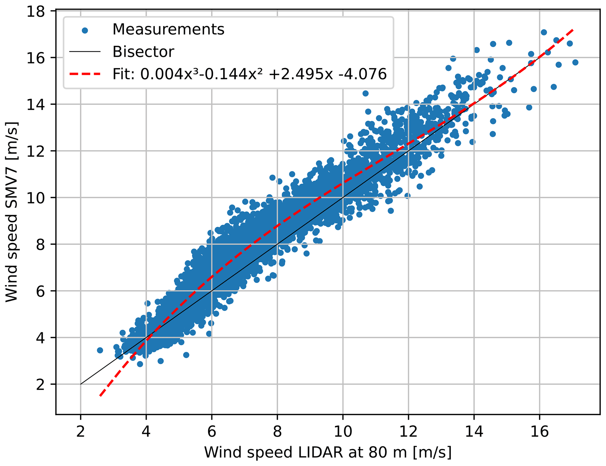
Figure 5Comparison of wind speed measured by the Windcube lidar at 80 m height and the nacelle wind speed of SMV7 in the sector 170–195∘. Fit statistics performed by P5: R2 = 0.94, σ=0.54 m s−1.
As for the wind shear, a constant value of 0.25 was used, which corresponds to the average of the shears measured by the Windcube v2.
Finally, the complete data set was binned over wind speed and wind direction in bins of 1 m s−1 and 1∘ respectively so as to further reduce the measurement noise and speed up the tuning process.
Tuning parameters and process. The velocity deficit was modelled with the kinematic Gaussian velocity deficit model by Bastankhah and Porté-Agel (2014) and the root sum of squared deficits superposition model (Katic et al., 1986). Wake-added turbulence was modelled with the Crespo and Hernández (1996) turbulence model and deflection through the Bastankhah and Porté-Agel (2016) deflection model. The model calibration parameters that describe the wake velocity and wake turbulence models were further corrected in the tuning process, whereas for the wake deflection model the default FLORIS values were used. In addition to that, the exponent n of the cosine law (Eq. 1) used to model the power losses of yawed turbines was set to 1.88, i.e the value adopted by Gebraad et al. (2016).
As the incoming wind is permanently affected by the local orography and vegetation, it is necessary to account for the long-term spatial variability of both wind speed and wind direction. To achieve that, a heterogeneous flow field is parameterized in terms of shape functions and associated unknown speed-up (ΔWS) and wind direction (ΔWD) nodal values (Schreiber et al., 2020). The nodes were placed at the coordinates of the turbines, and the resulting mesh was further discretized for five different inflow wind directions. This resulted in seven nodes for each of the considered inflow wind directions (WD-20∘, WD-175∘, WD-195∘, WD-220∘, and WD-350∘), leading to a total of 35 speed-up and 35 wind direction nodes. The desired flow correction is then obtained by mapping the nodal values, with associated linear shape functions, to the locations of interest. The distribution of the nodes in terms of location and direction can be seen in Fig. 6a, which also depicts the resulting background flow field for an inflow speed of 7.56 m s−1 and a wind direction equal to 214.7∘.

Figure 6(a) Wind speed and direction node locations within the cluster. (b) Identified speed-up (ΔWS) nodal values. (c) Identified wind direction (ΔWD) nodal values.
The intrinsic parameters of the adopted wake and turbulence sub-models were identified together with the heterogeneous flow nodal quantities, resulting in a site-specific coupled simultaneous correction and tuning of the model. This ill-conditioned optimization problem was solved by mapping the unknown parameters into an orthogonal space via the singular value decomposition (SVD), solving the identification by a maximum likelihood estimation in the reduced space and then mapping back the solution to the physical space (Schreiber et al., 2020). The identified, tuned parameters for the wake model are shown in Table 6, while Fig. 6b and c show the identified speed-up and wind direction nodal values. For further details on the description of model parameters, see NREL (2021). For further discussion on the significance of such a parameterization, see e.g. van Beek et al. (2021).
2.2.3 P6
Atmospheric conditions at the site. The provided SCADA data covering the calibration period were used to model the site’s characteristics and perform preliminary comparisons.
Wind direction. The wind rose obtained from the calibration period data is similar to the one shown in Fig. 2 and contains a large portion of data for which no yaw offset is reported (about 65 %), whereas the remaining 12046 data points report a yaw offset. The ranges of wind direction that occurred during the provided blind test SCADA data are reported in Table 2. The yaw offsets during the calibration phase (calculated as the difference between the Windcube v2 lidar directional data at hub height and turbine SMV6’s nacelle-corrected heading) have a mean value of −13.3∘, with values ranging from −26 to +30∘.
Wind speed. The only available source of wind speed for both the calibration data set and the blind test data set is the nacelle-mounted anemometers at each turbine, if the Windcube v2 lidar is excluded. Preliminary correlations between the lidar's and turbine SMV6's wind speed signals showed a non-linear relationship and significant amount of scattering, suggesting the underestimation of wind speeds by the nacelle-mounted anemometers, especially for wind speeds lower than 10 m s−1 (as measured by the lidar). As explained in the next section, transfer functions have been used to convert wind speeds from anemometers to free-stream wind speeds using the measured active power and the provided warranted power curve. Additionally, directional correlations between different turbines have been used to obtain a table of wind speed corrections that represent the variation in wind speed at the site (also known as speed-ups). It is also stressed that any estimation of the wind farm blockage effect has not been attempted.
Atmospheric turbulence intensity. The variation in turbulence intensity with wind speed is shown in Fig. 7 as measured from both the lidar and turbine SMV6. Both the mean and the P90 turbulence levels in the two plots show some similarities, especially for wind speeds above approximately 7.5 m s−1. Although the correlation between the wind speed standard deviation at the lidar and SMV6’s nacelle-mounted anemometers shows significant scattering (not shown here), using the 10 min averaged wind standard deviation from the SCADA data is considered to be broadly suitable in this case for the purpose of wake modelling, as also pointed out in Duc et al. (2019). It is noted that the SCADA wind speed standard deviation data have not been used to obtain any turbine-specific turbulence intensity correction across the site, as was done for the wind speeds.

Figure 7Turbulence intensity (%) measured by (a) Windcube v2 at 80 m and (b) turbine SMV6 vs. wind speed (m s−1).
Air density. Historical atmospheric data have been obtained from ERA5 and NEWA reanalysis data sets at the closest available nodes to the site. The long-term averaged air density at the site was found to be 1.23 kg m−3, with values ranging between 1.13 and 1.35 kg m−3. These values have been used to correct the power curve in the simulations (see below).
Wind shear. The lidar measurements were provided at different heights and for a period of about 8 months. The two measurements closest to the low tip and high tip of the rotor (40 and 120 m respectively) have been used to estimate the average shear profile across the turbine rotor. Assuming the directional wind shear estimations at the lidar location are representative for all turbine locations (except for the directions with the wake effects), power-law exponents 0.178 and 0.268, respectively corresponding to wind direction bins centred at 0 and 210∘, have been used for the blind test simulations based on each case's wind direction range (see Table 2).
Calibration of turbine characteristics. The first step for the calibration process was to focus on data representative of normal operations only by filtering out any data recorded when yaw misalignment was present. The variation in wind speeds across the turbine locations was pragmatically estimated from correlations between the turbines' SCADA data, only from the two main directions of interest for the blind tests, in Table 2. In order to exclude the sectors with the wake effects and have enough data points, the SCADA wind speed signals at each turbine were filtered for broader directional sectors around the aligned directions with the wake effects. By using SMV1 and SMV6 as reference turbines for the north and the south wind direction cases respectively, correlations between each turbine and each reference turbine were performed for the filtered wind directions, in order to find speed-up factors describing the local variation in free wind speeds for the directions of interest. The obtained values were used to define these effects for the excluded directions with the wake effects, by averaging the valid directional values. An example of this approach is given in Fig. 8.
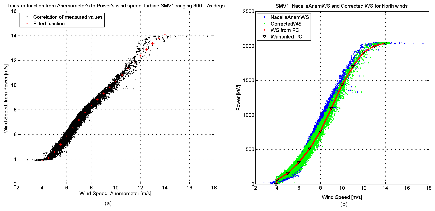
Figure 8(a) Rotor effective vs. nacelle anemometer wind speed (m s−1): Fitting between anemometer and power-based wind speeds at turbine SMV1 for northern wind speeds under rated power. (b) Power (kW) vs. wind speed (m s−1): comparison at turbine SMV1 between warranted power curve (PC), power based on anemometer wind speeds, and corrected power curve using the transfer function as described.
The turbine’s wind speed standard deviation values were assumed to be representative of the free atmospheric conditions, as described in the previous section, and have therefore been used for the definition of turbulent intensity.
Plotting the active power against the wind speeds from the nacelle-mounted anemometers for each turbine, large differences emerge when compared to the provided warranted power curve. The wind speed could be back-calculated from the active power SCADA signal; however, this signal is only provided for the calibration data set and not as part of the blind test package. Since at least one turbine’s SCADA wind speed signal was made available for each blind test scenario, the available calibration data set was used to create a transfer function linking nacelle anemometers' measurements and wind speeds back-calculated from active power, exclusively for the wind directions of interest. This was achieved, for each turbine, by using a sixth-order polynomial fitting process for SCADA wind speeds ranging between cut-in and rated wind speeds, hence covering the whole wind speed range in all the blind test scenarios analysed.
In order to calibrate the power curves from the available data recorded when yaw misalignment was present, the data were binned for different yaw angle ranges. Due to the limited amount of data recorded during the yaw misalignment tests, it was decided to focus specifically on three misalignment angles, −7, −13.3, and −18∘, deemed to be representative of the distribution of measured yaw misalignment angles during the blind tests. A power curve for each of these angles was obtained by fitting the data clustered in these three bins, and the thrust curves were also adapted to the yawed cases by applying the same wind speed shift found for the power curves. It is noted that the commonly used approach of modifying the power and thrust values by multiplying these by a factor such as cos(Ψ)n (where n is a positive real number and Ψ is the turbine yaw angle, as shown in Eq. 1) has not been used in this instance, also due to the large uncertainty given by the large range of exponent values found in literature. For completeness, a comparison between the calibrated power and thrust curves and the best-fitting cosine exponents (respectively being found to be 1.7 and 1.2) is shown in Fig. 9 for wind speeds of 6, 7, and 8 m s−1.
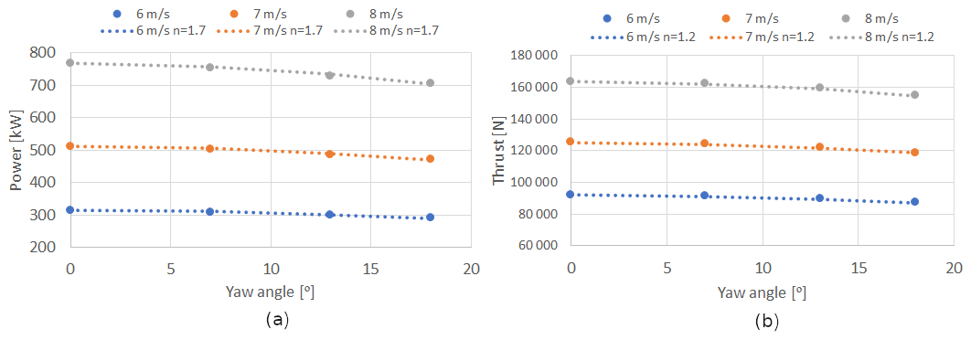
Figure 9(a) Power and (b) thrust values obtained from data calibration at three wind speed values and at four yaw misalignment settings, compared to a cos(Ψ)n function.
Wake modelling. Different wake modelling approaches have been tested for this specific site. The chosen steady-state model utilized, in a time-series fashion, for producing the results presented in this report is based on the Ainslie model (Ainslie, 1988), including modifications suggested by Anderson (2009) and Ruisi and Bossanyi (2019). The wake-added turbulence was modelled using the Quarton and Ainslie (1990) model, and for the superposition of wake effects the sum of deficits method is used for the velocity deficits, and sum of variances is used for turbulence superposition. The time series of air densities has been used to correct the power curve during simulations, as prescribed by the IEC standards. The rotor-averaged quantities have been calculated by taking into account the directional wind shear across the rotor, as explained in the previous section. Furthermore, it is noted that the effects of wind farm blockage, atmospheric stability, and veer have not been taken into account for the purpose of wake modelling at this site.
The model used for this simulation is the one by Bastankhah and Porté-Agel (2016), where the four numerical parameters used in the model were not calibrated (hence were kept the same as reported in the original article); however an additional factor of 2 is added to the formula predicting the skew angle in Eq. (6.12) in Bastankhah and Porté-Agel (2016) (as implemented also in FLORIS NREL, 2021). This version of the model was preferred to the same model with the exclusion of this additional skew factor, or the model by Jimenez (Jiménez et al., 2010) for which the characteristic parameter k was set to 0.05 (as opposed to 0.15, as suggested in the original article), based on previous experience with other calibration data sets.
2.2.4 P16
P16 results are obtained using an in-house wake modelling code. The calculations are based on single-wake superposition with the Bastankhah and Porté-Agel (2016) wake model, capable of modelling yaw deflection. The model parameters are optimized based on the provided calibration data set under normal SMV wind farm operation, using the SGA optimizer of the “pygmo” library (Biscani and Izzo, 2020). For the optimization run, the data were filtered for wind directions coming from the north, reflecting the multiple-wake case. Influences of orography and forest, resulting in an in-homogeneous wind field, were not taken into account. Wind speed, wind direction, and TI values from the upstream turbine (SMV1) were directly used for the definition of the ambient wind field. The parameters of the wake model were obtained by minimizing the sum of the average quadratic differences between power measurements and simulated power at every turbine of the wind farm. The following parameters were results of the optimization and used for further modelling: ka=0.234, kb=0.0037 and α = 4.967, β=0.0015. Those are principally the same model parameters as described for the other participants in Table 6, described in detail in Bastankhah and Porté-Agel (2016), but implemented in a different framework than FLORIS. Measurement uncertainties were not taken into account for the model calibration. We expect the high value of α, compared to literature studies, to be a reflection of the general uncertainty, especially of the wind direction measurement. As a large α leads to quite short near-wake lengths, which are essential for the magnitude of wake deflection in the deflection model, we expect the wake deflection with these parameters to be quite inefficient. For the yawed turbine, the power loss is modelled via Eq. (1) with n=1.88, and the change of CT with yaw is modelled analogously with an exponent of n = 1. This assumption was made due to the unknown behaviour of the turbine in yaw and based on Fleming et al. (2014).
Since there is no general agreement in literature, we expect the modelling of the turbine performance in yaw to be a large uncertainty factor. The multiple wakes are superposed via the quadratic sum of their deficits, and the rotor effective wind speed is calculated as the weighted sum at 19 points over the rotor. The wake-added turbulence intensity is modelled with the Frandsen (2007) model. Figure 10 shows the relative power of SMV2 compared to SMV1 for the data which were used for calibration of the model. In general, the mean wake losses show a good agreement with the measured data considering that the spread of the measured data is naturally higher due to measurement uncertainties.

Figure 10Comparison of measurements and P16 model outputs for calibration period, SMV2 compared to SMV1. The y axis shows relative power of SMV2 and SMV1, and the x axis indicates the incoming wind direction in (∘). Solid lines are the binned average of the measurements and model results indicated as scatters.
2.2.5 P17
Wake model description. A modified Gaussian wake model named Gaussian-IQ, which provides three-dimensional wake characteristics including wake width, velocity deficit, added turbulence (Ishihara and Qian, 2018), and wake deflection caused by yaw offset (Qian and Ishihara, 2018), is utilized by P17. Parameters that govern the evolution of wake in the Gaussian-IQ model are determined as the function of thrust coefficient and local hub-height turbulence intensity. No additional calibration of model parameters has been added, and the default values were utilized. To combine velocity deficits of multiple wakes, the rotor-based linear sum (RLS) is employed. For turbulence intensity in the multiple wakes, it is formulated based on the principle of a linear sum of square (LSS) with an additional correction term to consider the effects of wake interaction (Qian and Ishihara, 2021).
Turbine model description. The theoretical power and thrust curves of Senvion MM82 at the site are used to determine the turbine performance under normal operating conditions for an air density of 1.225 kg m−3. For the steered turbine, to model the power loss and thrust force change due to the yaw misalignment, an effective wind speed is introduced to power and thrust look-up tables, following the approach recommended by Ruisi and Bossanyi (2019), feeding into Eq. (1) as , where Ψ is the yaw offset angle and n is the yaw loss exponent set to 1.88, which is the value suggested by Gebraad et al. (2016).
Simulation process. The wind farm simulation is performed in steady state, and results are provided via a data set binned over wind speed and wind direction (WD) in bins of 1 m s−1 and 5∘ respectively. For each wind speed, the binned values with respect to, for example WD = 5∘, are obtained by taking the average of the results from 10 simulations of WD = 2.5∘. The wind speed, wind direction, and turbulence intensity (TI) in the axial direction are assumed to be homogeneously distributed in the wind farm. A wind shear profile following the power law with a constant exponent of 0.15 is applied to the inflow wind speed. As shown in Fig. 7, the variation in turbulence intensity with wind speed measured by the free-stream turbine SMV6 is quite stable for wind speeds above approximately 4 m s−1. Thus, the ambient turbulence level at hub height is set to be constant with the mean value of TI = 0.11.
2.3 Validation data pre-processing
The wind farm field data blind tests are prepared as single and multiple wakes, where the upstream turbine SMV6 was steered with −13.3∘ mean with respect to the incoming south-westerly wind. The results are evaluated in terms of balanced energy gains, as defined in Fleming et al. (2019). Since the experiments were not realized in the form of a toggle test, the baseline case is taken by considering two 2-month periods before and after the field tests, as shown in Fig. 11.
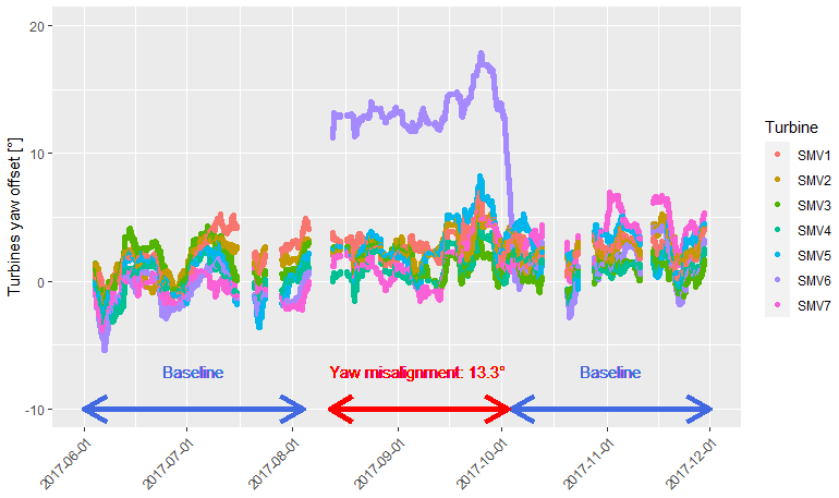
Figure 11Evolution of the yaw offset of all turbines in the farm during the period of the analysis. The reference wind direction is taken from the Windcube lidar. To smooth out the time series, a moving average of 3 d was applied. The periods corresponding to the baseline case and the wake steering case are marked by the arrows. The averaged misalignment angle on the SMV6 turbine is indicated.
The wind speed and direction reference signals for computing the energy ratios come from the Windcube v2. Due to the proximity of this sensor with the controlled turbine, the atmospheric conditions measured should be very similar to the ones faced by SMV6. The reference power signal is issued from the SMV7 wind turbine, which is the only remaining upstream turbine for the southerly wind sector. However, SMV7 is located very close to the forest and therefore experiences a much disturbed wind compared to SMV6. Consequently the SMV7 active power signal must be corrected to be representative of SMV6 in the baseline situation. This is done following the same procedure as explained in Simley et al. (2021); namely under normal operation, SMV6 and SMV7 active power signals are binned against wind speed (1 m s−1 bins) and wind direction (calculated every degree on overlapping 10∘ bins). Then, a transfer function is estimated by dividing the SMV6 averaged power by SMV7 averaged power in each bin. Finally this transfer function is applied to SMV7 power time series to generate a reference power signal used in both the baseline and the wake steering cases for the computation of the energy ratios.
2.4 Single-wake results
For the single-wake case, the estimated and observed performance of the SMV6–SMV5 turbine pair is investigated within a narrow wind sector of 200–215∘ (i.e. ±7.5∘ around the perpendicular direction), where the upstream turbine SMV6 is misaligned for 13–15∘ anticlockwise (negative misalignment with mean ∘). The final data set within that sector for wake steering consists of 216 10 min data points, while the normal operation data set used to calculate the baseline wake effect is made of 1120 10 min data points (484 recorded in June and July 2017, 616 recorded in October and November 2017).
2.4.1 Time-series comparison
For the submitted time-series results from P4, P5, P6, and P16, the predicted and observed power values at the upstream and downstream turbines are compared in Fig. 12. The root-mean-square errors are normalized (NRMSE) by 2050 kW rated power of the turbines. For the upstream turbine, SMV6, with wake steering control (or yaw misalignment) of −13.3∘ mean anticlockwise, P4 and P16 are seen to underestimate the power production for lower wind speeds. On the other hand, P5 seems to overestimate the SMV6 turbine power for higher wind speeds, around the transition between Regions II and III. P6, however, is seen to have a very good agreement with the observed power at the controlled SMV6 turbine upstream, though potentially with a slight under-estimation.
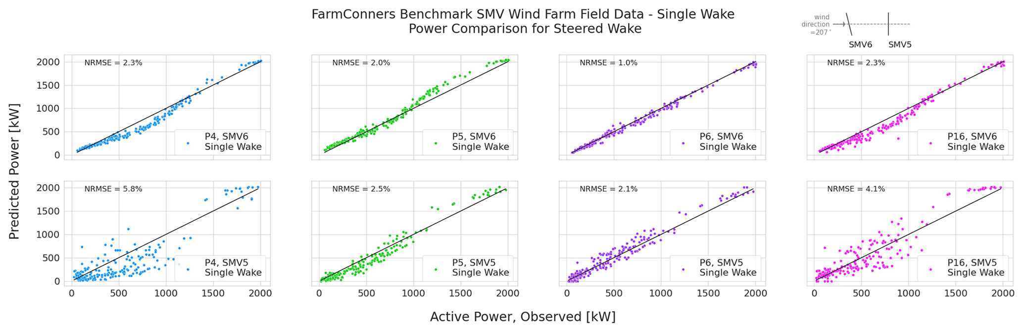
Figure 12SMV wind farm (WF) field data, single wake under wake steering power comparison per participant. Upstream (top row) turbine power under wake steering control of −13.3∘ misalignment, downstream (bottom row) turbine power under the steered wake – field observations vs. participating model predictions. Representative layout with corresponding yaw control set point is illustrated at the upper right corner.
At the downstream turbine under a steered wake, SMV5, the variance around the power predictions is notably higher for the steady-state models, potentially driven by the wake-added turbulence. The underestimation trend by participants P4 and P16 continues at SMV5 power comparisons as well, although a lesser discrepancy is observed for P16 results.
As stated earlier, the calibration data set the participants were provided for the wind farm field blind tests is limited to normal operation conditions. The limited calibration data surely affect the performance of all the participating models. This impact is arguably the most visible for P4 and P5, where the same WFFC-oriented platform is utilized. Between P4 and P5, the difference in the comparison for both the upstream and downstream power predictions is expected to be driven by the prior calibration and the final selection of the parameters for the controlled periods. Specifically, the implemented yaw loss exponents n = 3 for P4 and n = 1.88 for P5 (see Table 6) are argued to be the main factor for the difference observed in the upstream power predictions, especially compared with the recent field calibration at the same site under WFFC, discussed in Simley et al. (2021) where wind-speed-dependent (or indirectly CT) values of n≈2.2–2.3 for wind speeds between 4 and 8 m s−1, n≈1.3–1.35 for 8–12 m s−1, and n≈0.36 for 12–14 m s−1 are reported. In that regard, Fig. 12 highlights the sensitivity of the widely adopted WFFC-oriented models to the employed parameters and the importance of comprehensive calibration data and process. It also shows the significance of clear parameter descriptions for overall reproducibility of the results.
2.4.2 Binned quantities of interest: energy ratio and power gain
To analyse the effect of wake steering on the two-turbine wind farm (SMV6 as upstream, SMV5 as downstream), a similar methodology to that described in Fleming et al. (2019) is followed. Accordingly, both the observed power and the estimations by the participating models are distributed over ±0.5 m s−1 wind speed and ±2.5∘ wind direction bins. Per bin, the energy ratio, REnergy, is calculated via Eq. (2) with weighted summation, where N is the total number of wind speed bins per sector, ωi represents the weights per bin, is the mean of the total wind farm power per bin (either the normal operation/baseline power or power under wake steering WFFC) and for the single-wake case , and is the gross production averaged per bin, i.e. the power of the wind farm without the wake losses ( for single-wake case).
The weights per wind speed bin, ωi, aim to compensate for the non-equivalent number of samples within the “yaw misalignment” and “baseline” periods (see Fig. 11) in energy ratio estimation. Accordingly, they are assigned via the relative density of the samples within the respective bins. Therefore, the wake observed under normal operation (referred to as “Normal Wake : baseline”) and the gross production PRef have identical weights (both sampled under baseline period), where the observed and estimated wakes under WFFC have higher weights to compensate for a shorter yaw misalignment period in the data set. As an indication of uncertainty around the energy ratios, the standard deviation of the total power per wind speed bin is propagated, assuming the numerator and denominator of Eq. (2) are uncorrelated. Detailed description of the weighting strategy and the energy ratio calculation as well as the simplified uncertainty propagation can be found at the post-processing notebook published at the open-access FarmConners benchmark repository (Göçmen et al., 2021). It should be underlined that the resulting distribution of the model results considers only the variance in the time-series samples within the bin and is therefore simplistic and potentially conservative. A comprehensive analysis including input and model (parameter) uncertainties and their propagation is left as future work.
Figure 13 shows the energy ratio, REnergy, during the normal operation (or baseline) as well as under wake steering WFFC as observed on the field or estimated by the participating models (P4, P5, P6, P16, P17), per wind direction bin. Especially in the close-to-perpendicular wind sector, where , it can be seen that the steered wake is observed and estimated to be more energetic (i.e. higher REnergy), indicating a positive energy gain. The behaviour and the scale of the observations are in line with the recent field test results from the same SMV wind farm (Simley et al., 2021). For the participating models, the agreements are significantly better in the close sector. However, the variations notably increase at the wake border around 215∘. For the first wind sector centred around 200∘, all the models are seen to overestimate the energy ratios compared to the observations. The overall agreement becomes much better closer to the wake centre at the 205∘ bin, where P16 has a slight over-estimation. In line with the power scatter plots in Fig. 12, P4 notably underestimates the energy ratio for the remaining two sectors, where P5 and P6 have similar and overall very good agreement with the observations, and P16 has mostly good agreement except of the significant under-estimation around the wake border at 215∘. Note that for P17, where only the pre-binned quantities of interest were submitted, Fig. 13 includes only the mean REnergy. Based on the mean quantities, P17 is observed to slightly overestimate the energy ratios for almost all the sectors analysed.
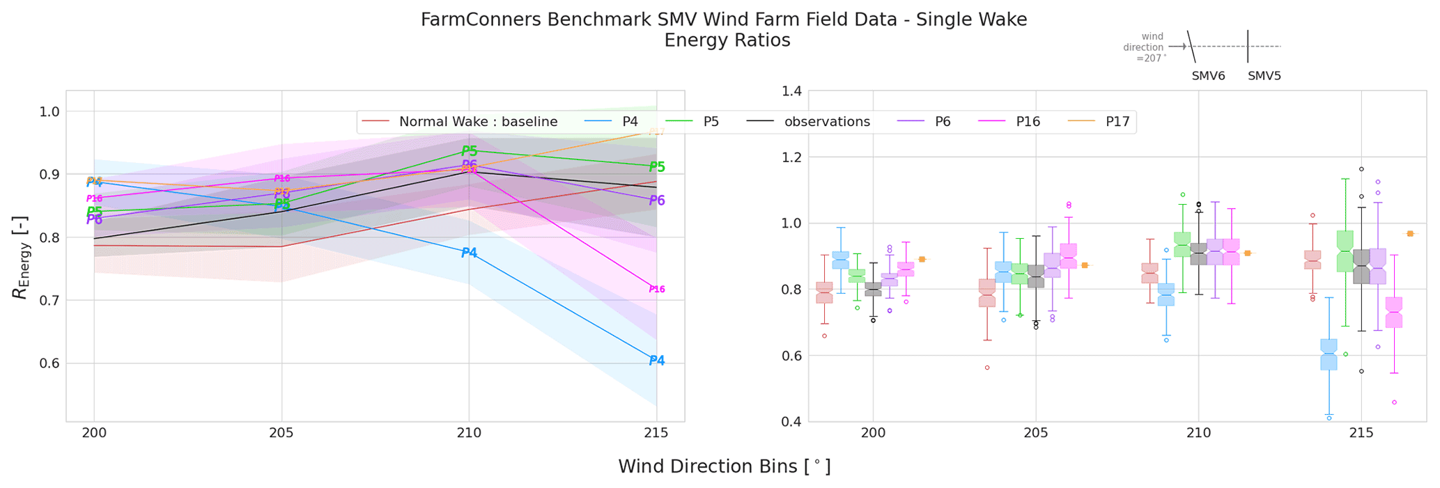
Figure 13SMV WF field data, single wake under wake steering – energy ratio comparison under wake steering control with −13.3∘ upstream misalignment. Representative layout with corresponding yaw control set point is illustrated at the upper right corner.
The power gain observed at the field and estimated per participant in the blind test is then calculated following Eq. (3), where the energy ratio computed in Eq. (2) during normal operation, is subtracted from the energy ratio under wake steering flow control . The uncertainty around the power gain is quantified via propagating the uncertainties of and estimated in Eq. (2).
Figure 14 compares the power gain under wake steering WFFC observed at the SMV wind farm and estimated by the participating models in the blind test. The boxplots show that for the close wake sector, i.e. , a positive power gain with 13–14∘ yaw control at the upstream turbine has above 75 % likelihood. In fact, the likelihood of more than 5 % gain in power exceeds 50 % in the same wind sector. However, around the borders of the wake, for the bins centred at 200 and 215∘, loss of power is equally as likely as a potential gain, indicating the importance of uncertainties for the risk assessment of WFFC implementation, also as underlined in Hulsman et al. (2020). Observably, the participating model behaviours for the power gain estimations follow the discussions on REnergy for Fig. 13. However it should be noted that P17 power gain now has a variation around its estimation, driven from the standard deviation of the energy ratio for the normal operation, in Eq. (2). With that, the over-estimation trend is down-scaled, and a better agreement can be argued for larger sectors >200∘.
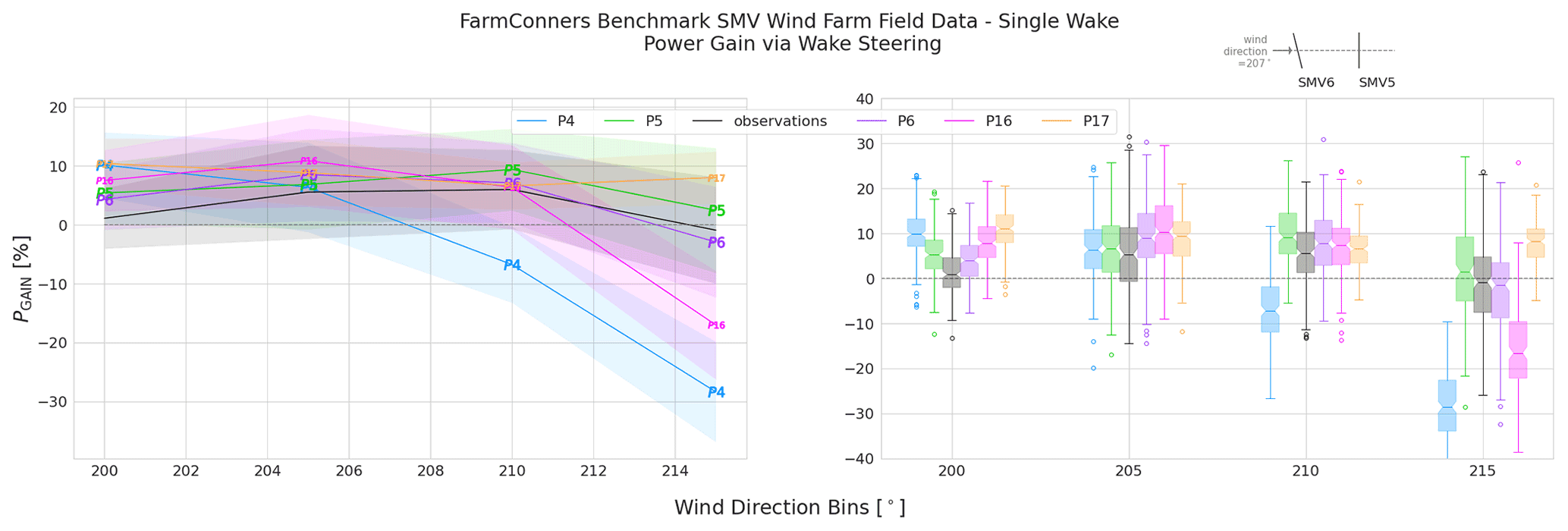
Figure 14SMV WF field data, single wake under wake steering – power gain comparison under wake steering control with −13.3∘ upstream misalignment. Representative layout with corresponding yaw control setting is illustrated at the upper right corner.
2.5 Multiple-wake results
For the multiple-wake case, the estimated and observed performance of the SMV6–SMV1 downstream turbines is investigated within a larger wind sector starting from 180∘ up to 215∘, so that effects of the wake steering at SMV6 can also be observed at the turbines further downstream of SMV5. Due to the imperfect alignment of the farm layout, it must be noted that this does not correspond to a multiple full wake effect; instead it is most probably a combination of overlapping partial wakes. Furthermore, for wind directions close to 180∘, the misaligned turbine SMV6 is in the wake of SMV7. Given the uncertainty in the evaluation data set, mainly driven by the layout of the wind farm, the multiple-wake results of the wind farm field data blind tests are presented in Appendix A.
2.6 Summary of the wind farm field data blind test
Although it is the key priority for advancing wind farm control technology (van Wingerden et al., 2020), the field test and validation for WFFC-oriented models are significantly challenging due to the stochasticity, non-stationarity, high variability, and overall uncertainty. Specifically for the FarmConners benchmark, the highlights of the participating model performance for the wind farm field data blind test can be summarized as below.
-
Similar models, disparate behaviour. In this blind test, several participants implemented similar models to resolve the wake behaviour behind a steered turbine (as listed in Table 3). However, even for the same framework utilized by P4 and P5, the results are seen to notably differ. This indicates high model sensitivity to the employed parameters and emphasizes the importance of the calibration procedure, as also analysed for another wind farm by van Beek et al. (2021). It also underlines the significance of clear methodology description and parameter listing for reproducible and credible estimations of the potential benefits of the technology.
-
Importance of the calibration data set. In the wind farm field data blind test, the calibration data were confined to the normal operation periods. This was mainly due to the limited availability of the controlled operation, which is typically the case for the majority of the operating wind farms. However, the blind test results show how crucial the information regarding the power loss at the controlled turbine(s) and basic downstream behaviour is to be able to customize the low-cost, control-oriented models under low observability of inflow conditions and turbine response.
-
A better wake steering implementation at the field. Given the high sensitivity of the parameters on the prediction of the gains observed, it can be concluded that the wake steering solution in practice would/should not be designed solely based on normal operation data. It would/should rather follow an iterative process in which a priori strategy can be developed and implemented based on normal operation tuning or standard, recommended, or off-the-shelf parameter values. After a certain period of data collected (e.g. a few months), the model parameters could be updated and a posteriori strategy (with a new set of optimal yaw control set points) can then be defined. Such a process could continue until a satisfactory agreement is reached between the model results and the observations.
This blind test builds upon a set of high-fidelity simulations performed in the context of the European R&D project CL-Windcon (CL-Windcon, 2016). They were performed with NREL's open-source SOWFA simulation package (NREL, 2012), which is a set of computational fluid dynamics (CFD) solvers based on OpenFOAM (2013), boundary conditions, and turbine models represented through the OpenFAST simulation tool (Jonkman, 2017). The scenarios consist of two different layouts (see Fig. 15), for the 10 MW INNWIND.EU reference turbine (INNWIND.EU, 2013): (i) three turbines with a 3 × 1 configuration (3WT) and 5 D distance among turbines where the third turbine has 0.5 diameters (D) lateral displacement with respect to the flow, and (ii) nine turbines with a 3 × 3 configuration (9WT) and 7 D distance among the turbines. The numerical verification tests are presented in Doekemeijer et al. (2018), and further details on the simulation setup can be found in Gomez-Iradi et al. (2019) and Doekemeijer et al. (2019).
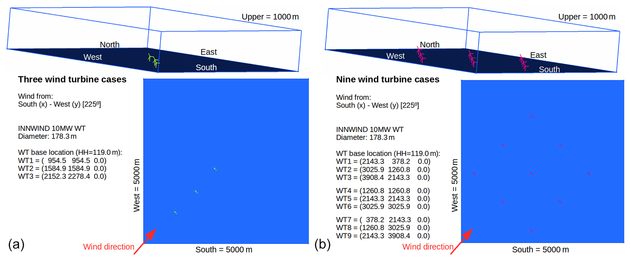
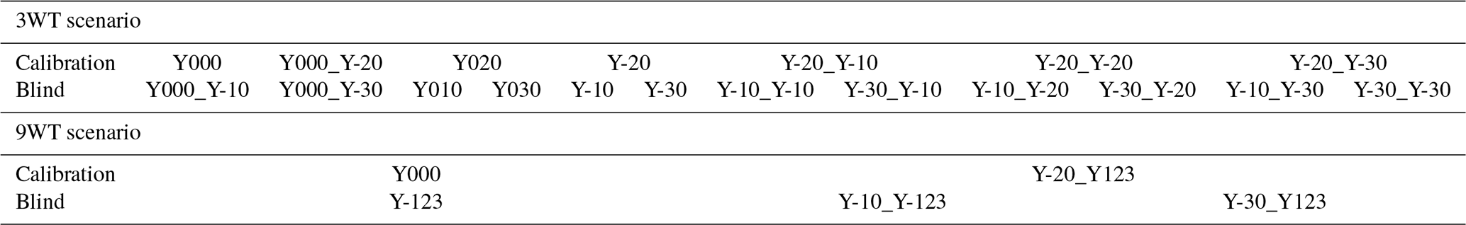
For the whole data set, combinations of three wind speeds, turbulence intensities, and roughness lengths were applied together with varied wind turbine control settings. However, for the specific blind test in FarmConners benchmark, an inflow corresponding to an average wind speed of 7.7 m s−1, turbulence intensity of 5.39 %, and roughness length of 0.001 m was selected (referred to as A4 in the original database CL-Windcon, 2019). The CL-Windcon LES blind test is among the most diverse and comprehensive in terms of the wake steering control strategies applied within the FarmConners benchmark. The yaw misalignment was varied in the range of ±30∘ for the first and/or the second row of turbines; see Table 7 for particular control settings among the 3WT and 9WT scenarios. The direction for the yaw convention, as well as the distribution of the control set points among the turbines, is illustrated per investigated case in the presentation of the results later in Sect 3.2 and 3.3.
Table 7Yaw misalignment control settings for the calibration and blind test for CL-Windcon LES cases. Yxxx: the downstream turbines are not misaligned where xxx [∘] indicates the yaw misalignment of the upstream turbine(s) (WT1 for 3WT scenario; WT1, WT4, and WT7 for 9WT scenario). Yxxx_Yyyy: upstream and the first downstream turbines are misaligned, where xxx [∘] and yyy [∘] indicate the yaw misalignment of the upstream and downstream turbines respectively. For 9WT scenario, xxx or yyy = −123 indicates −10, −20, and −30∘ yaw setting at turbines WT2, WT5, and WT8 respectively.
Targeted test cases explore a single full wake and multiple wakes under wake steering WFFC. Available data cover power production, hub-height, and/or rotor effective wind speeds at the turbines, as well as several structural loading variables, namely flap-wise root bending moment, total shaft bending moment, and total tower bottom bending moment. However, the load channels are excluded from the analysis in this study, and the participating models are evaluated based on the reported power production with and without WFFC.
3.1 Participating models
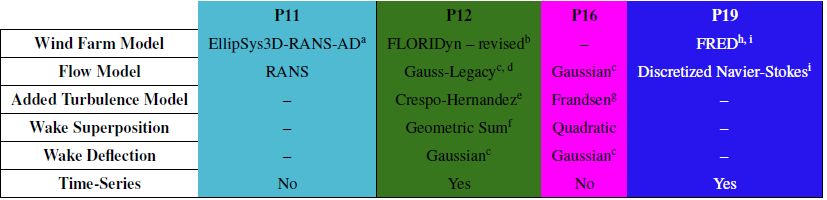
Within the FarmConners benchmark, the CL-Windcon LES blind test has had four participating models in total (IDs = P11, P12, P16, P19). Two steady-state and two (quasi-)dynamic models have been utilized for the exercise, covering a wide range of model fidelity. Table 8 lists their main characteristics for an easy comparison, especially for the lower-fidelity models. Further details of the implemented models are presented in the following sections.
Table 8Overview of the participating WFFC-oriented models, CL-Windcon LES blind test. a Sørensen (1995). b Becker et al. (2022a) and Becker et al. (2022b). c Bastankhah and Porté-Agel (2016). d Bastankhah and Porté-Agel (2014). e Crespo and Hernández (1996). f Shao et al. (2019). g Frandsen (2007) – IEC 2019 standard. h van den Broek (2021). i van den Broek and van Wingerden (2020) and van den Broek et al. (2022).
3.1.1 P11
P11 uses PyWakeEllipSys (DTU Wind Energy, 2021), which consists of the elliptic Reynolds-averaged Navier–Stokes (RANS) solver EllipSys3D (Sørensen, 1995). The numerical setup is similar to the one in Larsen et al. (2020), where the wake deflection was also studied. The turbines are modelled by Joukowsky actuator disks (no nacelle or tower is modelled), and the disc-averaged normal velocity is used to control each turbine using 1D momentum theory. The wind turbine data needed for the AD model, i.e. CT(UH,∞), CP(UH,∞), and TSR(UH,∞), are taken from the DTU 10 MW report by Bak et al. (2013).
Turbulence is modelled with the closure of van der Laan et al. (2015), and the inflow follows neutral atmospheric surface layer profiles. These profiles are prescribed to match the free-stream velocity and total turbulence intensity at hub height: UH,∞ = 7.7 m s−1 and IH,∞ = 5.4 % (the “A4” wind case of the CL-Windcon campaign used in the FarmConners benchmark).
3.1.2 P12
The parametric WFFC model used for this benchmark study by P12, also detailed in Becker et al. (2022a) and Becker et al. (2022b), will be referred to as FLORIDyn (FLOw Redirection and Induction Dynamics model). The central idea of FLORIDyn is to approximate the dynamic wake behaviour of wind turbines in a wind farm with low computational cost by piece-wise updating the steady-state flow field with a new steady-state description which fits the new states. This update from the precursor FLORIS model (see Doekemeijer et al. (2020)) is driven by observation points (OPs), which are created and updated at the rotor plane for each time step. They represent the influence of the turbine state travelling downstream. Within FLORIDyn, the steady-state wake is modelled via FLORIS (NREL, 2021), which is then propagated through the wind farm, instantly affecting turbines downstream. For instance, when the yaw angle of the turbine changes, the new generation of OPs will copy the new angle while old OPs still travel according to the previous angle. In the case of overlapping wakes, an OP travels into the wake of another turbine. It locates the closest upstream and downstream OPs from the foreign wake and interpolates their reduction factor at its location. The calculation of CT and CP is based on the lookup table generated via SOWFA (NREL, 2012) high-fidelity simulations for the reference turbine in the blind test. For the current benchmark study, the statistical properties of the wind field are matched (mean wind speed and turbulence intensity); however, no specific calibration to match to the CL-Windcon LES wake data was performed. Calibration using uncertainty quantification is intended to form part of a future publication.
3.1.3 P16
For the P16 results, the same in-house wake modelling tool as described in Sect. 2.2.4 is used. It consists of a Gaussian-based wake model (Bastankhah and Porté-Agel, 2016) with a quadratic single-wake superposition model. Based on the calibration data provided, the wake model parameters , and βd are also optimized with the SGA optimizer of the “pygmo” library (Biscani and Izzo, 2020) and the same loss function, i.e. the sum of the average quadratic differences between the calibration states power and simulated power at every turbine of the wind farm. However, the optimization procedure is different compared to the SMV wind farm field data blind test. Instead of using a single global wake model parameter for all turbines, here each turbine has independent wake model parameters which are determined by the optimizer. The power loss and the dependency of CT on the yaw angle are modelled by factors (cos Ψ)n, with the same values for n=1.88 as described in Sect. 2.2.4 and Eq. (1). For the power and thrust curves a lookup table that was derived from the BEM model of the 10 MW DTU reference turbine is used.
3.1.4 P19
The dynamic WFFC model used for this benchmark study by P19, currently under development (van den Broek, 2021), will be referred to as FRED (Framework for wind farm flow Regulation and Estimation with Dynamics). For the sake of brevity, a concise description is presented here, and interested readers may refer to van den Broek and van Wingerden (2020) and van den Broek et al. (2022). The model is based on Navier–Stokes equations that are discretized in time and a finite-element method that is used for spatial discretization with the Taylor–Hood element (Wieners, 2003). Dirichlet boundary conditions (Givoli and Keller, 1989) prescribe the inflow velocity. The inflow boundaries are dynamically chosen based on the wind direction. For example, for the current blind benchmark case where the wind flows from the south-west direction, the south and west boundaries are marked as inflow. The other boundaries are given Neumann conditions (Givoli and Keller, 1989), by default. The model is initialized with a uniform flow field given by initial velocity and a constant pressure. A generalized mixing length (Morgan et al., 1977) model is used to model the sub-grid-scale eddy viscosity. The wind turbine forcing on the flow is approximated using an actuator disc model. For the current benchmark study, the statistical properties of the wind field are matched (mean wind speed and turbulence intensity); however, no specific calibration to match to the CL-Windcon LES data was performed. Calibration is intended to form part of our future works.
3.2 Single-wake results
To have a generic comparison for both the single and multiple-wake results for two time series and two steady-state results submitted, exclusively the mean quantities of interests estimated by the participating models are presented in the CL-Windcon LES blind test results. Accordingly, the mean power per turbine, PTi, submitted by the participants under WFFC and normal operation are used to calculate the power difference per turbine, ΔPTi, and power gain, PGAIN, by Eqs. (4) and (5) respectively:
where P is the power and Ti is the turbine ID within the wind farm configuration (T0 for upstream, T1 for downstream in the single-wake case).
Figure 16 shows ΔPTi and PGAIN for a single wake with 5 D spacing where the upstream turbine, T0, is misaligned +10∘ (Y010), −10∘ (Y-10), +30∘ (Y030), and −30∘ (Y-30). For PGAIN in Fig. 16, the boxplots represent the distribution of the reference high-fidelity simulations at each control setting, where the mean PGAIN estimated by the participating models is illustrated on top. For ±10∘ misalignment at T0, CL-Windcon LES shows that the likelihood of power loss (up to more than 5 %) is higher than the gain for the investigated two-turbine configuration. This is relatively well captured by P11, P16, and P19, where P12 overestimates the potential of the control strategy. However, for larger upstream misalignment, the agreement between the participating models and the validation data set generally declines. For +30∘ steering at T0 (clockwise rotation), the low likelihood of the power gain is closely estimated by P16, and P11 and P19 indicate over-estimation of the wake losses, and the general trend of high-gain predictions from P12 continues. The asymmetry in the wake behaviour is significant when investigating the −30∘ steering set point, which is likely to be caused by wake rotation and/or wind veer combined with the upstream misalignment. This is, although less pronounced, also observable for ±10∘ and not represented by the participating models for either of the control settings. For the −30∘ upstream steering, the potential of the power gain exceeds 5 % in CL-Windcon LES results, which is relatively well captured by P12 and significantly underestimated by the other models. These rather pessimistic gains reported at −30∘ steering can be further analysed by ΔPTi in Fig. 16. There, it is seen that the upstream power loss is represented fairly well by all the participating models (within ±1 standard deviation bounds), but the wake losses behind a misaligned turbine are overestimated by the majority of the models, except for P12. This can potentially be explained by the less wake deflection produced by the models, as e.g. studied previously for P11 (Larsen et al., 2020). The same trend is visible in the other high-fidelity simulations within the benchmark as well, as can be seen in the TotalControl LES blind test in Sect. 4.2, for high degrees of upstream misalignment in P11 and P16 results.
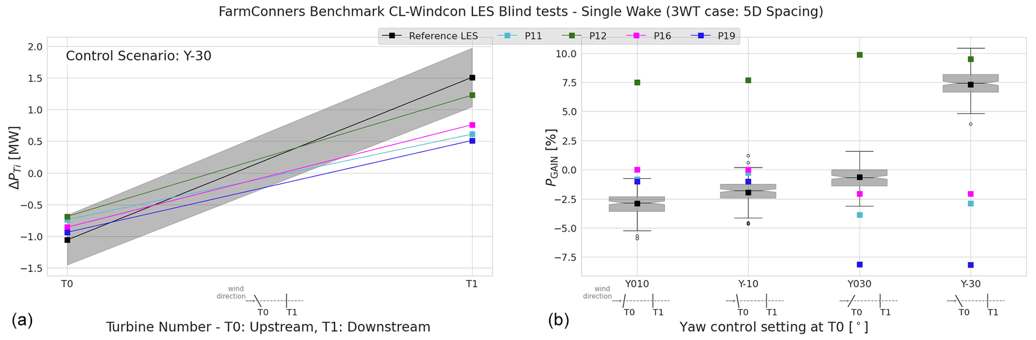
Figure 16CL-Windcon LES blind tests, single wake under wake steering for the three-turbine configuration (3WT) with 5 D spacing. (a) Power difference (mean) in absolute values (MW) per upstream (T0) and downstream (T1) turbine, when T0 is −30∘ misaligned (Y-30). (b) Power gain (mean) for the two-turbine subset of the wind farm (T0 + T1). Boxplots represent the distribution of the reference CL-Windcon LES time series per control setting where T0 is steered +10∘ (Y010), −10∘ (Y-10), +30∘ (Y030), and −30∘ (Y-30). Representative layouts with corresponding yaw control settings are illustrated along the x axes.
Figure 17 investigates ΔPTi and PGAIN for a single wake, this time for the 9WT scenario with 7 D spacing where the upstream turbine, T0 is misaligned −10∘ (Y-10), −20∘ (Y-20), and −30∘ (Y-30). It should be noted that the control settings presented here in the 9WT single-wake cases are the subset of the Y-123 settings under the blind tests reported in Table 7, based on each row of turbines in Fig. 15. PGAIN in Fig. 17 shows an interesting trend where −10 and −30∘ upstream misalignments result in positive power gain but −20∘ indicates a potential power loss for the investigated two-turbine configuration in the reference CL-Windcon LES results. Compared to 5 D spacing in Fig. 16, −10∘ upstream misalignment produces more power at the 7 D downstream turbine, hence the positive power gain which is slightly underestimated by the participating models. The agreement for −20∘; however is significantly better for the majority of the models, which could be due to the same upstream control setting in the calibration data set, though the downstream yaw setting(s) are different (i.e. Y-20_Y123 in Table 7). The upstream power loss due to misalignment is more than compensated for by the −30∘ yaw setting in CL-Windcon LES results, as also seen in ΔPTi behaviour. However the downstream power gain is significantly underestimated by all the models, as also observed and discussed for 5 D spacing in Fig. 16 as well as under similar upstream control settings applied in TotalControl LES in Sect. 4.2 where P11 and P16 also participated.
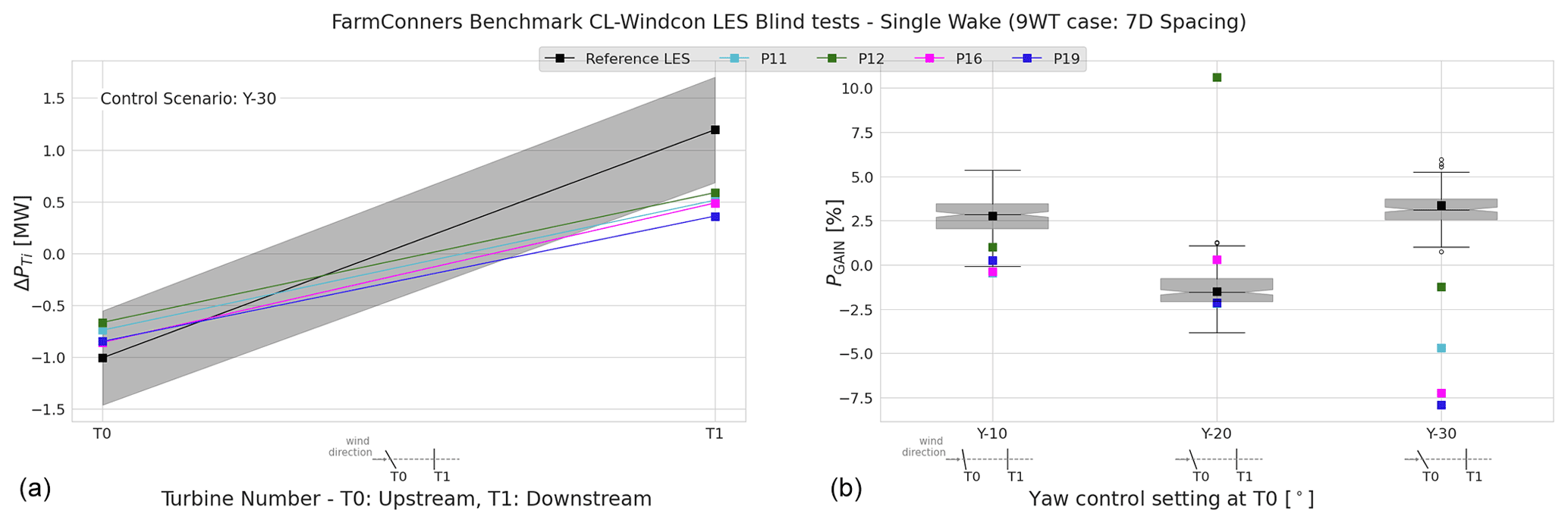
Figure 17CL-Windcon LES blind tests, single wake under wake steering for the nine-turbine configuration (9WT) with 7 D spacing. (a) Power difference (mean) in absolute values (MW) per upstream (T0) and downstream (T1) turbine, when T0 is −30∘ misaligned (Y-30). (b) Power gain (mean) for the two-turbine subset of the wind farm (T0 + T1). Boxplots represent the distribution of the reference CL-Windcon LES time series per control settings where T0 is misaligned −10∘ (Y-10), −20∘ (Y-20), and −30∘ (Y-30). Representative layouts with corresponding yaw control settings are illustrated along the x axes.
3.3 Multiple-wake results
Similar to the single-wake results, the mean power estimated by the participating models is compared with the CL-Windcon LES blind test database for the multiple-wake cases. Accordingly, the power difference per turbine and the wind farm level power gain via Eqs. (4) and (5) are presented in Figs. 18 and 19. The turbine IDs for multiple-wake cases, however, are WT1, WT2, and WT3 for the three-turbine configuration and WT1, WT2, …, WT9 for the nine-turbine configuration. The representative layouts as well as the turbine-specific control settings within the investigated wind farm configuration are illustrated on the x axes of Figs. 18 and 19.
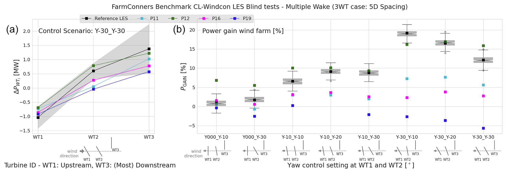
Figure 18CL-Windcon LES blind tests, multiple wake under wake steering for the three-turbine configuration (3WT) with 5 D spacing. (a) Power difference (mean) in absolute values (MW) per turbine, when WT1 and WT2 are both −30∘ misaligned (Y-30_Y-30). (b) Power gain (mean) per control setting in the three-turbine wind farm. Boxplots represent the distribution of the reference CL-Windcon LES time series per control setting listed in Table 7. Representative layouts with corresponding yaw control settings are illustrated along the x axes.
Figure 18 shows ΔPTi and PGAIN for three turbines with 5 D spacing (where WT3 is laterally 0.5 D apart) for several upstream and (first) downstream yaw control settings for the CL-Windcon blind tests listed in Table 7. For the investigated configuration, Fig. 18 indicates that the power gain is mainly driven by the control setting applied at the upstream turbine, WT1, where the misalignment of WT2 has a relatively lower impact. This is in line with other LES studies that investigate multi-turbine wake steering (e.g. Archer and Vasel-Be-Hagh, 2019). Especially with the lateral spacing of WT3, all the control cases where WT1, is misaligned indicate positive power gain up to more than 20 % in CL-Windcon LES runs. For all the participating models except P12, this trend is highly underestimated, and the agreement gets gradually worse with higher wake deflection. P12, however, estimates the behaviour relatively well, especially when WT2 is also misaligned. This can potentially be attributed to the high levels of wake deflection embedded in P12 model parameters. ΔPTi enables a closer look at the power difference at the individual turbine level for the highest degrees of control settings at WT1 and WT2, −30∘ each. There, similar to the single-wake analyses, it can be seen that the upstream losses observed in reference CL-Windcon LES at WT1 are relatively well represented by the participating models, but potential gain at the controlled downstream turbine (WT2) is underestimated by the majority. In addition to the under-representation of the wake deflection compared to the CL-Windcon LES, the difference in the power yaw loss exponent, n in Eq. (1), for the misaligned turbine in the wake can also play a role here, as demonstrated in Liew et al. (2020b). For the laterally spaced most downstream (WT3) turbine, the overall behaviour in the power performance is seemingly captured by all the participating models. However, significantly higher fluctuation in the expected power gain at WT3 should also be noted with approximately ±1 MW.
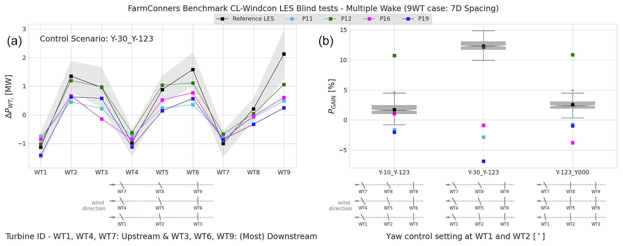
Figure 19CL-Windcon LES blind tests, multiple wake under wake steering for the nine-turbine configuration (9WT) with 7 D spacing. (a) Power difference (mean) in absolute values (MW) per turbine, for the control case Y-30_Y123 as shown in Table 7. (b) Power gain (mean) per control setting in the nine-turbine wind farm. Boxplots represent the distribution of the reference CL-Windcon LES time series per control setting listed in Table 7. Representative layouts with corresponding yaw control settings are illustrated along the x axes.
Figure 19 illustrates ΔPTi and PGAIN for the nine-turbine configuration with 7 D spacing in a regular layout consisting of three rows with WT1, WT4, and WT7 as upstream turbines. Similar to the previous results of the CL-Windcon LES blind test, the highest yaw control setting at the upstream turbines (Y-30_Y123) is observed to produce the highest PGAIN in the validation data set, up to 15 % for the nine-turbine layout. Again, PGAIN is underestimated by all the participating models except for P12, this time at higher discrepancies with up to 20 % less in the mean values. ΔPTi illustrates the disagreements in the power difference per turbine for that control setting, and the upstream power loss at −30∘ steered turbines WT1, WT4, and WT7 is reproduced well. The error in the most downstream power predictions, however, is significantly higher for all except P12 at the turbines WT3, WT6, and WT9. This is also in line with the behaviour previously discussed for the other configurations in the blind test where the upstream yaw setting is −30∘. As opposed to P12, the wakes behind less steered turbines (Y-10_Y-123 and Y-123_Y000) are better captured by P11, P16, and P19, with overall less sensitivity to the yaw setting at the second turbines in the rows WT2, WT5, and WT8. This also implies an overall stronger wake deflection reported in the CL-Windcon LES reference data set than the majority of the participating models.
3.4 Summary of the CL-Windcon LES blind test
Due to its capability of representing significant features of wind-farm flows, LES is an ideal choice for proof-of-concept studies regarding WFFC strategies. In that regard, with many control settings included, the CL-Windcon LES blind test provides a broad overview for the initial comparison of participating models. The highlights can be summarized as follows.
-
Higher steering, higher disparity. Although −20∘ upstream misalignment was in the calibration data set for the CL-Windcon LES blind tests, the overall participating model agreement is seen to be better for −10∘ upstream steering than −30∘. Further analysis indicate the main cause of this disparity to be due to deflected wake modelling rather than the upstream power loss at the controlled turbine(s). As the reference LESs suggest a higher likelihood of power gain for those control settings, the need for better deflection models and/or (even) a more comprehensive calibration data set with higher deflection angles should be considered.
-
Most upstream misalignment is the main driver for the expected power gains. Within the FarmConners benchmark, the CL-Windcon blind test provides a unique opportunity with its diverse control settings, including the misalignment of the downstream turbine(s). For the investigated layouts with 3 × 1 and 3 × 3 turbine configurations, however, it is seen that the misalignment of the second row of turbines has a relatively lower impact on the expected power gains, compared to the most upstream. Similar results are reported in other LES studies with multi-turbine yaw misalignment (e.g. Archer and Vasel-Be-Hagh, 2019).
-
Take all the conclusions with a grain of salt. As indicated earlier, high-fidelity simulations are very well suited for the proof-of-concept studies. Although it has many advantages, one of the main drawbacks of the reference CL-Windcon LES data set is its limited simulation period of 10 min. The impact of steering reported here and the overall model comparison (especially for the steady-state models), therefore, should be read as an initial comparison, not a comprehensive validation. Further discussion on the code comparison based on high-fidelity simulations is provided in the next section with the TotalControl LES blind test results.
This blind test is based on an extension of high-fidelity simulations performed as part of the Horizon2020 project TotalControl (TotalControl, 2018). The high-fidelity simulations have been performed using EllipSys3D (Michelsen, 1992, 1994; Sørensen, 1995), which is a finite-volume Navier–Stokes solver. The wind turbines are modelled using the actuator line method (Sørensen and Shen, 2002; Sørensen et al., 2015), which is fully coupled to the aeroelastic tool Flex 5 (Øye, 1996).
TotalControl defined a virtual reference wind farm (Andersen et al., 2018), which consists of 32 DTU10MW turbines (Bak et al., 2013) in an 8×4 grid with every other row offset in the streamwise direction. LESs were performed for different atmospheric conditions and wind directions, and a subset of the data is publicly available (Andersen and Troldborg, 2020). The selected case corresponds to a conventionally neutral boundary layer with a geostrophic wind of G = 12 m s−1, a roughness length of m, and a Coriolis parameter of s−1, which represents a latitude of 43.43∘; see additional details in Andersen et al. (2019). The resulting mean velocity at hub height is approximately 10.4 m s−1.
The wind farm layout for the two blind tests is shown in Fig. 20, where the turbine spacing is marked in red and the intentionally yawed turbines are marked in green boxes.
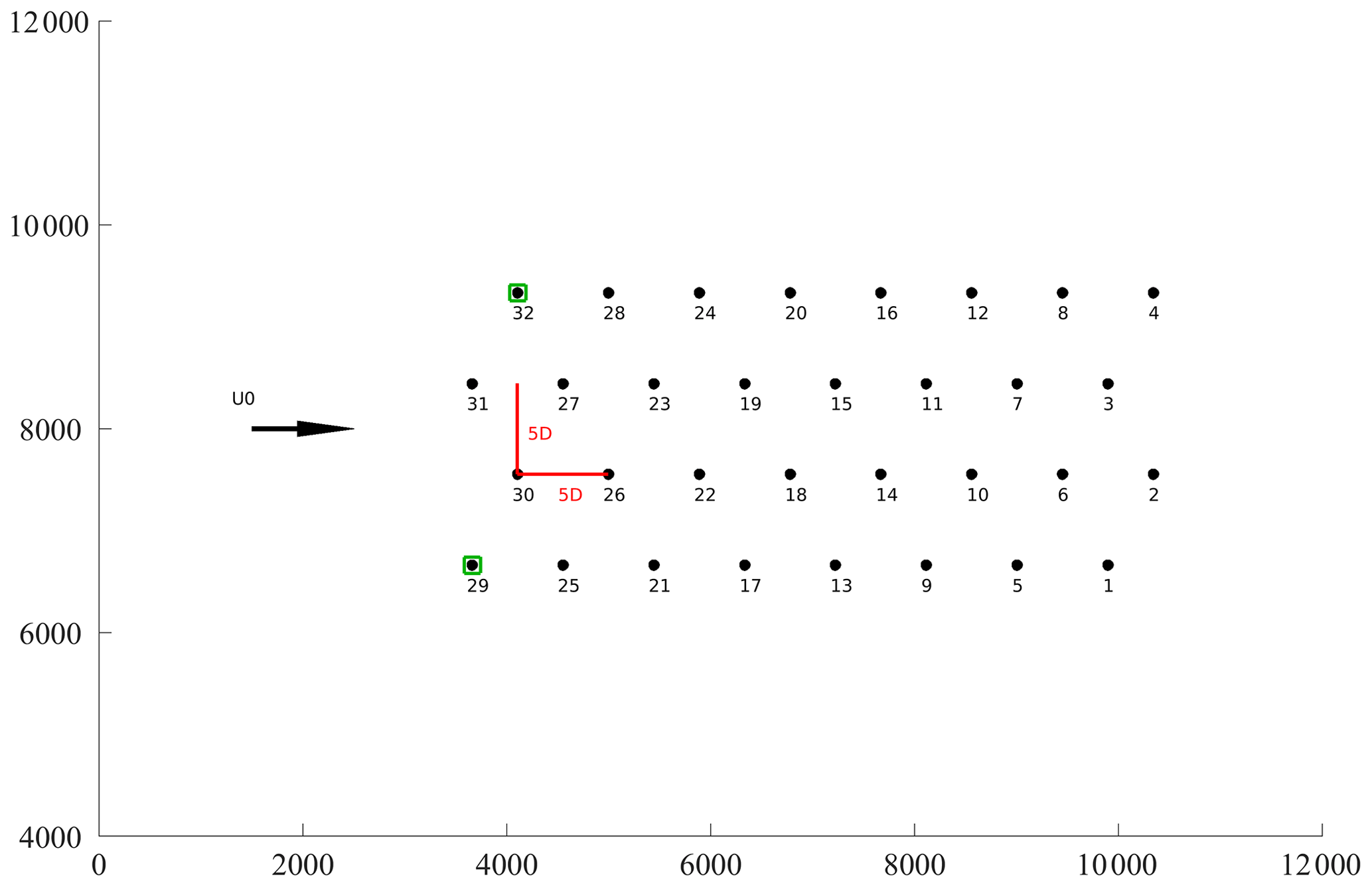
Figure 20Layout of the TotalControl reference wind farm with a wind direction of 90∘. Green squares mark yawed turbines. The turbine IDs are referred to as WT1, WT2, …, WT32 throughout the rest of the section.
An additional simulation was performed for the FarmConners blind test by intentionally yawing turbines WT29 and WT32 under the exact same inflow conditions. All simulations have been run for a total of 4500 s, where the initial 900 s of transient has been removed to have 3600 s of operation for the blind test.
Figure 21 shows a comparison of the power production during normal operation (in black) and steering (in red) for the two turbines in the single-wake scenario corresponding to a wind direction of 90∘. Clearly, the power production is reduced on the upstream turbine, when steering, while the power production increases for the downstream turbine operating in the steered wake. It is also evident how the normal operating turbines frequently reach rated power. Hence, this scenario is particularly challenging for a blind test as it is close to rated wind speed of the turbine of 11.4 m s−1, where correct representation of the turbine control is essential.
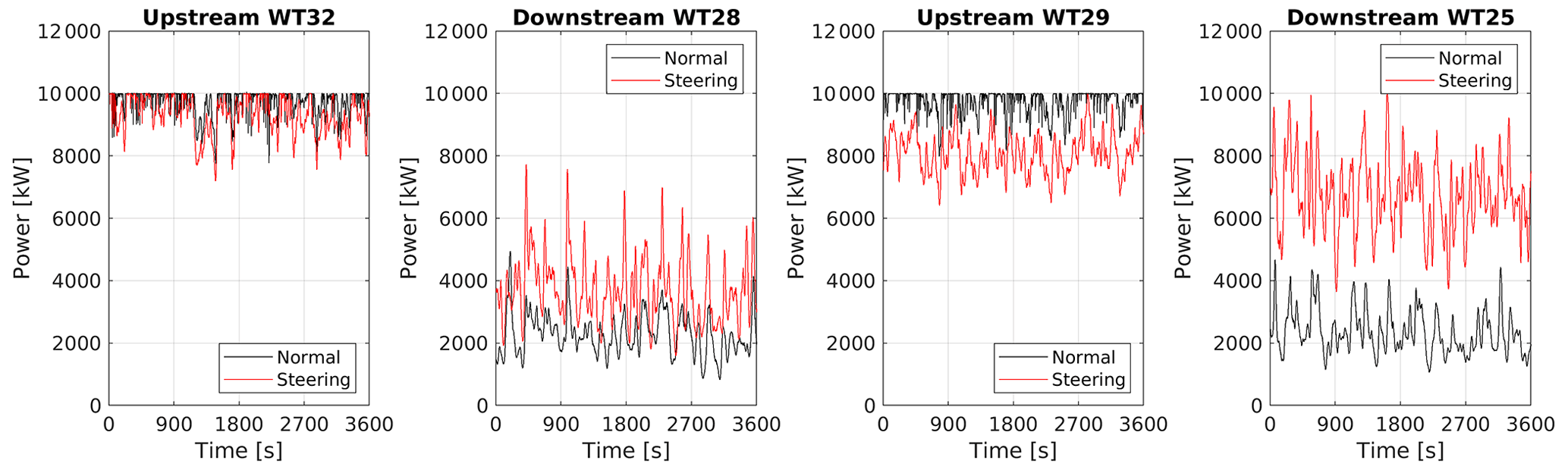
Figure 21Power time series for the single-wake scenario in the TotalControl LES blind test for the four turbines: WT32–WT28 and WT29–WT28. Black corresponds to normal operation, while red is power production during wake steering.
4.1 Participating models
Within the FarmConners benchmark, in total five models (P8, P10, P11, P16, P20) have participated in the TotalControl LES blind test. The participating models cover a range of fidelities for both the flow modelling and the turbine representation. The participating models and their calibration processes are briefly described in this section, where Table 9 summarizes the main characteristics of the models.
Table 9Overview of the participating WFFC-oriented models, TotalControl LES blind test. a Larsen et al. (2008) and Madsen et al. (2010). b Larsen et al. (2020). c Bastankhah and Porté-Agel (2016). d Poushpas (2016). e Niayifar and Porté-Agel (2016). f Frandsen (2007) – IEC 2019 standard. g Calaf et al. (2010), Allaerts and Meyers (2015), and Munters and Meyers (2018). h Sørensen (1995).
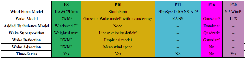
4.1.1 P8
The P8 methodology uses a preliminary version of HAWC2Farm to perform dynamic wind farm simulations on the blind test case. HAWC2Farm leverages the aeroelastic wind turbine software HAWC2 (Larsen and Hansen, 2007; Madsen et al., 2020) with the dynamic wake meandering (DWM) model (Larsen et al., 2008; Madsen et al., 2010). While HAWC2Farm typically uses HAWC2 as the underlying wind turbine software, this preliminary implementation uses HAWCStab2 data (Verelst et al., 2018) to synthesize a dynamic turbine model, from which the dynamic rotor induction is fed into the DWM model to generate the wakes. A flexible version of the DTU10MW is used to calibrate the rotor induction model to ensure the wake deficit is not overestimated, as described by Liew et al. (2020a). The wake passive tracers advect in all spatial directions based on large-scale turbulence. Wake deflection is modelled using a modified version of the DWM model, using a Hill's vortex method to simulate the lateral wake deflection. This method has shown good agreement with other wake deflection models as well as full-scale experiments (Larsen et al., 2020). The added wake turbulence model as defined by Larsen et al. (2008) was not activated in this investigation due to the absence of turbine loads; however, the wake dissipation model was adjusted continuously based on a windowed turbulence intensity sensor with a length of 500 s. Wake summation is performed by using only the dominant wake (i.e. largest wake deficit) at any point in space, followed by a further adjustment which was calibrated using the blind test data:
where and are the adjusted and unadjusted longitudinal wind speeds at location respectively; α(N) is a calibrated factor as a function of the number of upstream turbines, N; and ΔUi is the wind speed wake deficit of the ith turbine.
4.1.2 P10
The P10 model consists of wind turbine models based on the work of Neilson (2010), augmented with an individual blade model based on the work by Gala-Santos (2018). The wind turbine model is validated against DNV Bladed in Gala-Santos (2018). As an input, the wind turbine requires rotor-averaged effective wind speeds, which can be generated from input criteria of mean wind speed and turbulence intensity. The requirement for an effective wind speed rather than a point-wise wind speed means that the wind data are not identical as a time series to that used by the TotalControl LES results. However, the statistical properties of the flow are matched. A lateral wind speed is also generated that informs the meandering of wakes (see Poushpas, 2016). Whilst previous work involving the P10 model has used the Frandsen wake model (Frandsen, 2007), the wake modelling was recently updated using a the Gaussian wake model of Bastankhah and Porté-Agel (2014, 2016), adapted for effective wind speed modelling (including load impacts) via a similar methodology to the wind shear and tower shadow modelling in Gala-Santos (2018). Further additions are made to account for wake steering effects, though these use an empirical method. It is assumed that the reduction in power from a wake is cos 1.9(ϕ) based on Simley et al. (2020) (where ϕ is the yaw misalignment). In order to model this change in power via wind speed, an adjustment to the wind speed of with k=1.25 is applied. Though crude, this method has good agreement with the cos 1.9 power adjustment up to yaw angles of between 20 and 30∘. Beyond ensuring that the statistical properties of the wind field are matched (the same turbulence and mean wind speed), no specific calibration to match to the TotalControl LES data was performed. Note that the new wake model is intended to form part of a future publication.
It should also be noted that the controller used for the wind turbine differs from the DTU controller typically used for this turbine. Compilation issues prevented the DTU controller from being used, and so the turbine control strategy and basic controller detailed in Recalde-Camacho et al. (2020) are used instead.
4.1.3 P11
The numerical model, code, and turbine data are the same as described in Sect. 3.1.1. Free-stream velocity and total turbulence intensity at hub height used m s−1 and . These values are based on time and plane averages of the LES data in the region upstream of the wind farm. To save computational time and simplify the simulation, the whole TotalControl reference wind farm was not simulated (32 turbines as seen in Fig. 20), but only the relevant row of turbines (WT2, WT3, and WT8 respectively, depending on the case); hence lateral blockage effects are neglected in our simulations.
4.1.4 P16
For the P16 results, the calibration procedure is identical to the procedure described in Sect. 3.1.3 for the CL-Windcon results. More details on the wake models can be found in Sect. 2.2.4. The mean value of the time-series wind speed was used as input to our model, and the TI was derived from the mean and standard deviation.
4.1.5 P20
The P20 model is SP-Wind, an in-house large-eddy simulation code built on a high-order flow solver developed over the last 15 years at KU Leuven (Calaf et al., 2010; Allaerts and Meyers, 2015; Munters and Meyers, 2018). SP-Wind solves the three-dimensional, unsteady, and spatially filtered Navier–Stokes momentum and temperature equations, with wind turbines contributing to the forcing terms in the equations. Spatial discretization is performed in the horizontal and span-wise directions by using pseudo-spectral schemes while vertical fourth-order energy-conservative finite differences are used in the vertical direction. The equations are marched in time using a fully explicit fourth-order Runge–Kutta scheme, and grid partitioning is achieved through a scalable pencil decomposition approach. The turbines in the flow domain are parameterized using the aeroelastic actuator sector method (AASM) (Vitsas and Meyers, 2016). Subgrid-scale stresses are modelled with a standard Smagorinsky model with Mason and Thomson wall damping (Allaerts and Meyers, 2015).
Wind farm simulations are run for a period of 75 min, which includes a 15 min start-up period for the settling of initial transients. A previously developed inflow database (Munters et al., 2019a, b, c, d) is utilized to provide the inflow conditions for the wind farm through the concurrent precursor method (Stevens et al., 2014; Munters et al., 2016), and the entire wind farm is rotated in the flow domain to simulate different wind directions. The structural and aerodynamic properties of the DTU 10 MW turbine tower and blades and the DTU Wind energy controller are used to simulate the turbine operation (Bak et al., 2013).
4.2 Single-wake results
For the single-wake case within TotalControl LES blind tests, the model performances are compared for two-turbine subsets of the TotalControl reference wind farm in Fig. 20, with WT32–WT28 and WT29–WT25 for 90∘ incoming wind direction. In these two-turbine subsets, the upstream turbines WT32 and WT29 are misaligned for 20 and 30∘ anticlockwise respectively. The blind tests include 1 h simulations where the wake loss reduction, Δu in Eq. (7), and power gain, PGAIN in Eq. (8), are compared among the participating models. Note that both Δu and PGAIN are evaluated per model via the submitted controlled (WFFC) and normal operation results of the participating models.
where U is either the hub height or rotor effective wind speed that represents the spatially averaged wind speed over the rotor at the upstream, Uup, and downstream turbine(s), Udown.
where P is the power and i is the turbine ID in the investigated subset of the layout (two turbines for single-wake and eight turbines for multiple-wake analysis behind the controlled turbines WT29 and WT32 in Fig. 20).
Figure 22 shows the wake loss reduction for both WT32–WT28 and WT29–WT25 turbine pairs with −20 and −30∘ upstream misalignment (anticlockwise) respectively. The time series on the left is illustrated at the frequency of the wind speed signals for all the (quasi-)dynamic models, including the validation data set TotalControl LES. Notably high fluctuations are seen for both of the control settings in the validation data set, which are very well captured by P8 with 5 s resolution. P20 is also in relatively good agreement, where the observed dynamics in the validation data set is closely followed. For P10, the rotor effective wind speed is used throughout the model, resulting in much lower fluctuations compared to other dynamic models due to spatial averaging of the point-wise wind speed variation. Figure 22 boxplots indicate that all the models, including steady-state P11 and P16, suggest a better recovery when the upstream turbine is −30∘ yawed compared to −20∘, with up to 40 % reduction in median wake losses relative to normal operation. The uncertainty, however, should also be noted with large fluctuations in the dynamic simulations with WFFC in the two-turbine configuration with 5 D spacing.
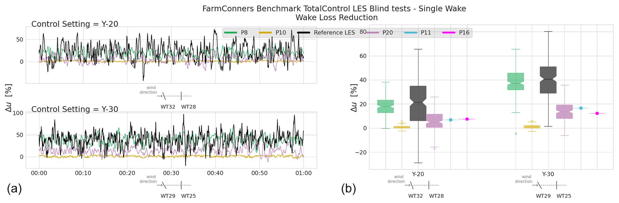
Figure 22TotalControl LES blind tests, wake loss reduction, Δu, for single wake under wake steering for two-turbine configurations with 5 D spacing (WT32–WT28 with 20∘ yaw and WT29–WT25 with 30∘ yaw at the upstream turbines). (a) Time series of Δu, illustrated at the submitted frequency by the participants, for both control scenarios. (b) The distribution of the Δu within the 1 h blind test period for both 20 and 30∘ anticlockwise yaw misalignment WFFC scenarios.
The transition from the wake loss reduction to the power gain comparison is highly affected by the turbine representation and the controller implementation of the participating models. Figure 23 highlights that clearly, especially considering the higher sensitivity of the power surface to the investigated wind speed interval around the rated region (as illustrated in Fig. 21). Although the wake recovery is captured very well by P8 as seen in Fig. 22, the positive reduction in wake losses does not translate to positive power gains for either of the control settings. Similar to P10, the power loss at the upstream turbine due to misalignment exceeds the power gain observed at the downstream turbine. The trend is further emphasized for higher-degree steering and potentially reinforced by under-representation of the power curve under normal operation downstream (shifted to the right). Here, it should be underlined again that the controlled settings were not included in the calibration data set distributed to the participants, and the mismatch in the upstream power loss can partially be attributed to that. See Appendix B for further analysis and illustration of the power difference per upstream and downstream turbine.
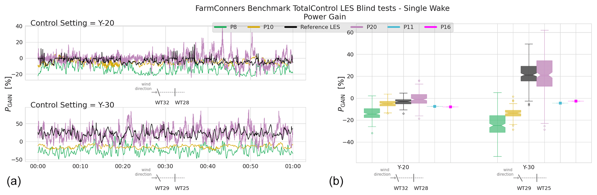
Figure 23TotalControl LES blind tests, power gain, PGAIN, estimations for single wake under wake steering for the two-turbine configurations with 5 D spacing (WT32–WT28 with 20∘ yaw and WT29–WT25 with 30∘ yaw at the upstream turbines). (a) Time series of PGAIN, illustrated at the submitted frequency by the participants, for both control scenarios. (b) The distribution of the PGAIN within the 1 h blind test period for both 20 and 30∘ anticlockwise yaw misalignment WFFC scenarios.
Figure 23 also shows that the only participating LES, P20, predicts similar levels of power gain overall with TotalControl LES, for both of the control scenarios. Although the reduction of the wake losses is underestimated in comparison, it is compensated for by lower power losses estimated at the controlled turbine upstream (see Fig. B1 in Appendix B for further details). The time series in Fig. 23 also indicate a faster controller response in P20, which results in a much larger spread around the reported PGAIN.
The steady-state results from P11 and P16 are in relatively good agreement for the lower degrees of misalignment at −20∘, but they underestimated the power gain likelihood for higher steering. This is indeed in line with their behaviour for similar control scenarios under CL-Windcon LES blind tests discussed in Sect. 3.2, where less wake deflection is produced by the models at higher steering as also observed in the wake loss reductions results in Fig. 22 above.
4.3 Multiple-wake results
Similar to the single-wake cases, 20 and 30∘ anticlockwise upstream yaw misalignment control scenarios for 90∘ incoming wind direction are investigated for the multiple-wake results in TotalControl LES blind tests. This time, eight-turbine subsets with 5 D spacing within the TotalControl reference wind farm are analysed, namely the rows WT29, WT25, …, WT1 and WT32, WT28, …, WT4 in Fig. 20. The layouts of these subsets as well as the corresponding control settings are illustrated in the presented results, i.e. the x axes in Fig. 24.
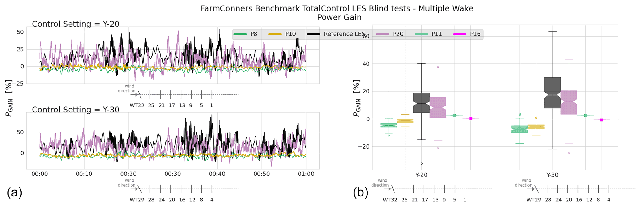
Figure 24TotalControl LES blind tests, power gain estimations, PGAIN, for multiple wakes under the upstream wake steering for the eight-turbine configurations with 5 D spacing (WT32–WT4 with 20∘ yaw and WT29–WT1 with 30∘ yaw at the upstream turbines). (a) Time series of PGAIN, illustrated at the submitted frequency by the participants. (b) The distribution of the PGAIN within the 1 h blind test period, for both 20 and 30∘ anticlockwise upstream yaw misalignment WFFC scenarios.
Figure 24 shows the power gain, PGAIN, of the eight-turbine, 5 D spacing wind farms under 20 and 30∘ anticlockwise upstream yaw misalignment WFFC scenarios. Compared to the single-wake results in Fig. 23, the fluctuation is seen to be much larger in the validation data set for multiple wakes, reaching up to 30 %. However, the trend in the median is similar with positive power gains for both of the WFFC scenarios, indicating higher likelihood under −30∘ upstream misalignment. This is closely captured by the other LES, P20, with highly correlated time series. Conversely, the other (quasi-)dynamic models underestimate the power gain, with a larger discrepancy for the higher steering. At least for P8, the overestimated power loss at the controlled turbine is argued to be the underlying reason, as also observed in the comparison of the single-wake results in Sect. 4.2 and Appendix B. Similarly for the steady-state models P11 and P16, the under-estimation of the power gain perseveres. However, the difference is less prominent as the effect of under-represented upstream wake deflection fades out with an increasing number of turbines along the row.
4.4 Summary of the TotalControl LES blind test
With additional participants, longer time series, simpler layouts, and focused control scenarios, the TotalControl LES blind test provides interesting comparison and supplementary discussion for model performance. Its highlights can be summarized as below.
-
Similar trends in the high-fidelity models. The TotalControl LES blind test hosts a unique comparison of two separate LES frameworks developed in different institutes. As stated earlier, comparison of lower-cost models against such tools (often referred to as numerical validation) is seen as a pre-requisite for their implementation in the field. Therefore, it is reassuring for the further adoption of the WFFC technology to have relatively good agreement with correlated dynamics between the two methodologies, as was observed in the TotalControl blind test, especially for the power gain results with different control scenarios in single and multiple-wake analysis.
-
Turbine representation and controller implementation. The TotalControl LES blind test showcases the sensitivity of the results to the turbine representation and the implementation of the controller. This was particularly emphasized via the translation of potential wake loss reduction to the power gains under WFFC. A prior study to compare (and calibrate if relevant) the power surfaces and controller operation under uniform flow is recommended for similar blind tests or numerical validation studies in the future.
-
Uncertainties and risk. Although it has longer time series compared to CL-Windcon LES blind tests, the TotalControl LES also replicates the conventionally neutral boundary layer. It does not include severe variability that might be observed in the field (e.g. Göçmen et al., 2020b) and corresponding uncertainties particularly for the wind direction. For the investigated scenarios, higher likelihood of benefits via wake steering control is estimated by the majority of the models in the blind tests. However, in particular the high-fidelity models indicate significant risk of inducing additional losses, given the probability of the power gain based on instantaneous values. Such trends are also discussed in Kheirabadi and Nagamune (2019), and their implications to operational risks under WFFC should be further evaluated by the end-users of the technology.
Here in this article we present Part I of the results of the FarmConners benchmark for code comparison under controlled operation. The benchmark brought together four data sets generated under several European WFFC projects: (1) SMV wind farm field data, (2) CL-Windcon wind tunnel experiments, (3) CL-Windcon LES, and (4) TotalControl LES databases, where data sets 1, 3, and 4 focusing on the large rotors are investigated in this study. The wind tunnel experiments are the focus of Part 2 of the series.
Although the original benchmark included more control strategies (i.e. axial induction) and quantities of interest (i.e. load channels), the analysis presented here is limited to wind speed and power behaviour under wake steering WFFC.
The results from 11 participating models in total are then presented separately under these three blind tests. The highlights of the blind test exercises are summarized individually in their corresponding sections through the article. A compilation of the observations/reference simulations and participating model trends for the overall benchmark is listed below.
-
Customizable WFFC-oriented models. The overwhelming majority of the participating models in the FarmConners benchmark are parametric, typically modular frameworks, indicating their popularity within the field. Using similar approaches to resolve the wake behaviour, the main difference among them is the calibration procedure. Accordingly, the importance of variety in terms of control set points in the calibration data set is underlined in all the blind tests. Similarly, a clear description of the calibration procedure with a list of parameters when disseminating the results is crucial for reproducible and credible assessment of the potential gains via WFFC.
-
Beyond flow modelling. The FarmConners benchmark also highlights the importance of turbine representation and controller implementation in realizable power gains via wake steering WFFC. A separate comparison and calibration of the power surfaces and controller operation for isolated cases are recommended prior to field implementation, as well as future blind tests or validation studies.
-
Overall a good agreement. Especially for well-calibrated models with a relatively good representation of the dynamics, the participating model agreement to the observations/reference simulations is seen to be reasonable for all the blind tests. This is particularly the case for smaller yaw control set points and lower (temporal and/or spatial) fluctuations in the inflow. Within the benchmark, two separate LES frameworks developed in different institutes are also compared, and high correlation observed in their results is found to be reassuring for the technology readiness level (TRL) of WFFC where high-fidelity simulations are considered to be the key enabler for further field implementation.
Although an already extensive analysis, the presented FarmConners benchmark results are limited in the applied control strategy and the investigated quantities of interest. It should therefore be read as the first step on which other benchmarks can be built. With increasing availability of field tests, wind tunnel experiments, and reference high-fidelity simulation databases, future work should include larger wind farms, different control strategies, and other control objectives such as potential load alleviation and profit maximization.
As discussed in Sect. 2.5, the multiple-wake cases for the SMV wind farm blind test results are deemed to be inconclusive. The main difficulty is the wind farm layout orientation and several partial wake scenarios included in the wider sector behind the controlled turbine. Nevertheless, the analysis is presented here for the interested parties, where the main outcomes in terms of the participating model performances are in line with the single-wake analysis of the same blind test presented in Sect. 2.4.
Due to its wider wind direction sector, the filtered data set for wake steering consists of 579 10 min data points (including the 216 points already used for the single-wake case), while the normal operation data set used to calculate the baseline wake effect is made of 1849 10 min data points (841 recorded in June and July 2017, 1008 recorded in October and November 2017).
A1 Time-series comparison
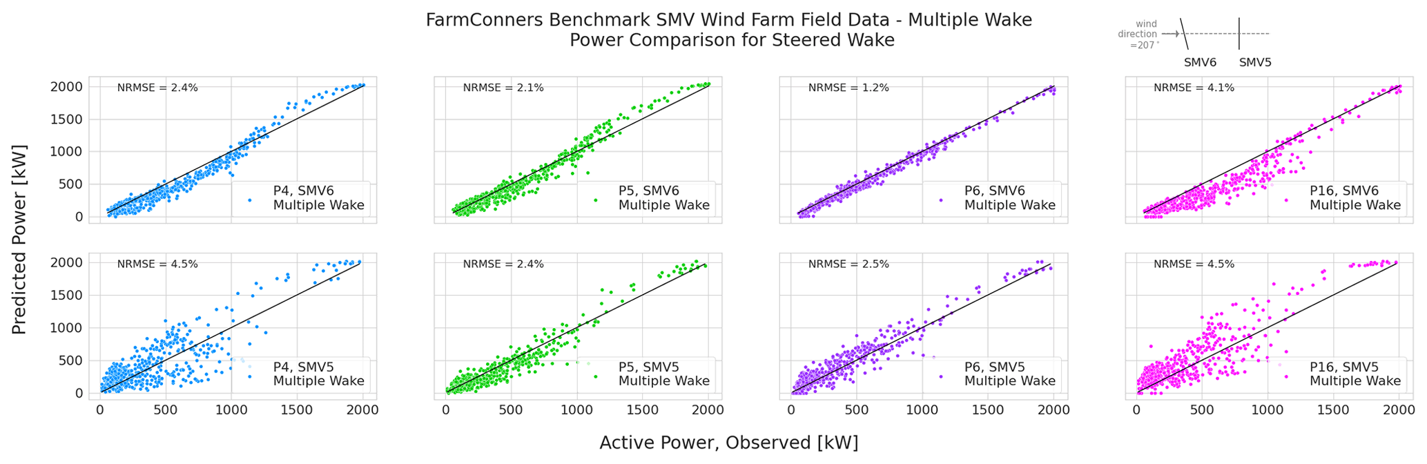
Figure A1SMV WF field data, multiple wake under wake steering WFFC with −13.3∘ upstream misalignment – power comparison. Representative layout with corresponding yaw control setting is illustrated at the upper right corner.
A2 Binned quantities of interest: energy ratio and power gain
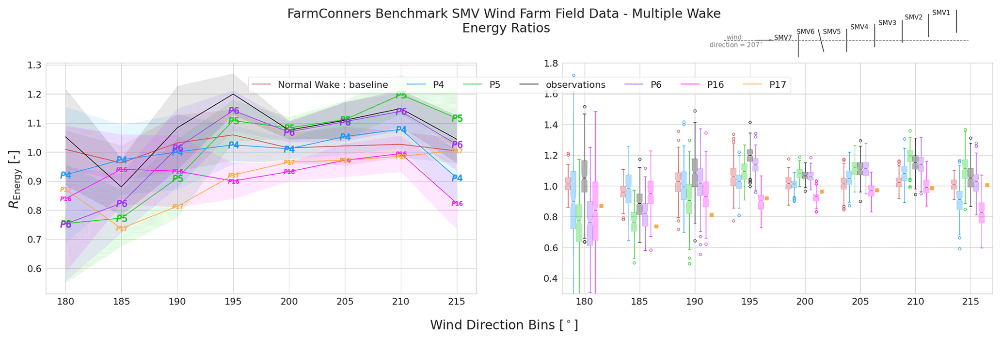
Figure A2SMV WF field data, multiple wake under wake steering WFFC with −13.3∘ upstream misalignment – energy ratio comparison. Representative layout with corresponding yaw control setting is illustrated at the upper right corner.
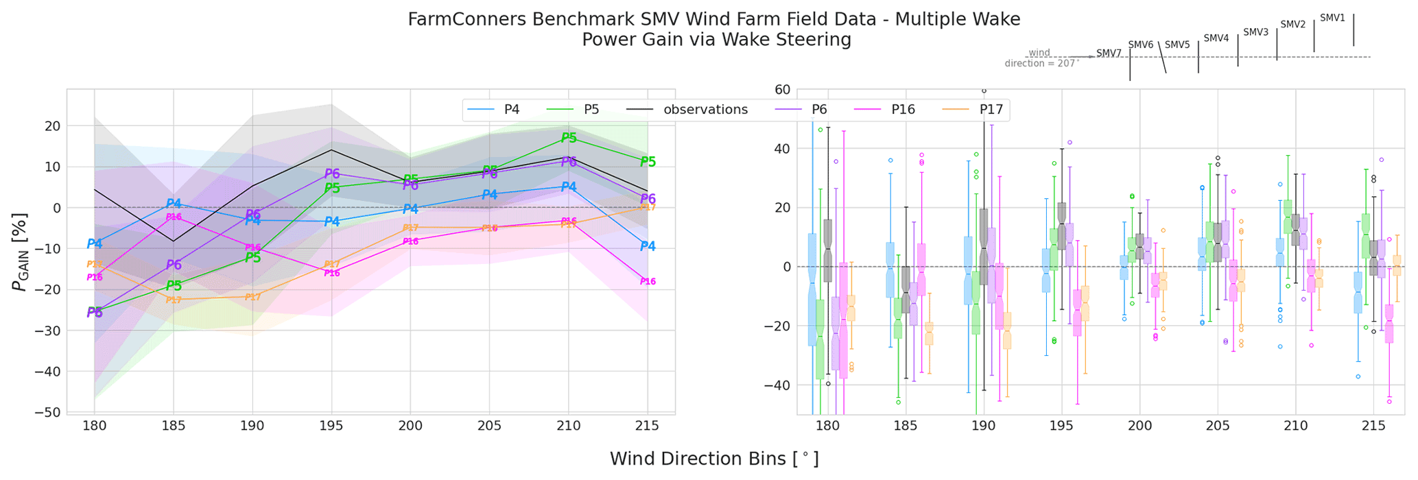
Figure A3SMV WF field data, multiple wake under wake steering WFFC with −13.3∘ upstream misalignment – power gain comparison. Representative layout with corresponding yaw control setting is illustrated at the upper right corner.
In order to analyse the participating model behaviours further, power difference, ΔP in Eq. (4), per turbine is compared for upstream (WT32 and WT29) and downstream (WT28 and WT25) turbines and is illustrated in Figs. B1 and B2 below respectively. They show the differences in the representation of the controlled and normal operation turbine power surface, where the former was not included in the calibration data set. This analyses supports the discussions carried out under Sect. 4.2 and aims to distinguish the underlying reasons of the model behaviours in terms of power gain, particularly in Fig. 23. It further highlights the differences in the controller implementation and turbine representation, given the sensitivity of the results to the blind test. It should also be noted that P10 submitted the time series for Pratio directly and is therefore excluded in the illustrations below.
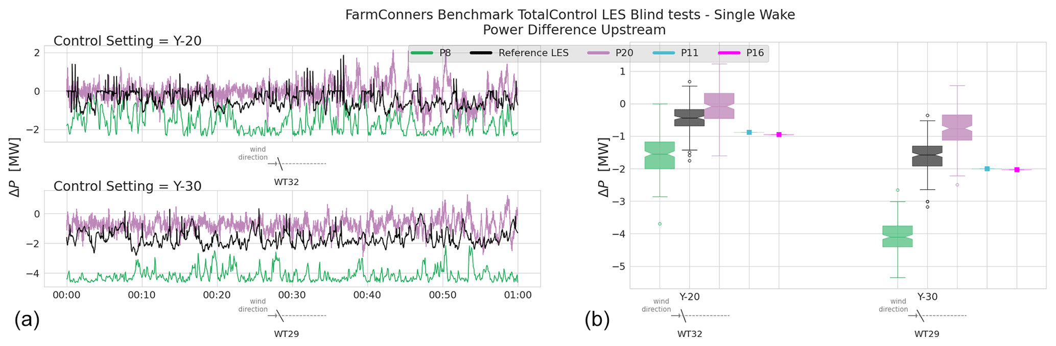
Figure B1TotalControl LES, single wake under wake steering power difference, ΔP, comparison for the upstream turbines WT32 (−20∘ yaw) and WT29 (−30∘ yaw). (a) Time series of ΔP at the upstream turbines illustrated at the submitted frequency by the participants. (b) The distribution of ΔP within the 1 h blind test period. For both 20 and 30∘ anticlockwise yaw misalignment WFFC scenarios.
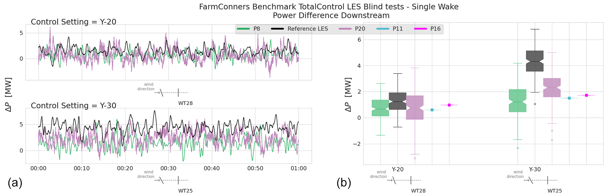
Figure B2TotalControl LES, single wake under wake steering power difference, ΔP, comparison for the downstream turbines WT28 (behind −20∘ yawed turbine) and WT25 (behind −30∘ yawed turbine). (a) Time series of ΔP at the downstream turbines illustrated at the submitted frequency by the participants. (b) The distribution of ΔP within the 1 h blind test period. For both 20 and 30∘ anticlockwise yaw misalignment WFFC scenarios.
The notebooks for the blind test results, including data snippets, can be obtained via the public repository of the FarmConners benchmark (Göçmen et al., 2021, https://doi.org/10.5281/zenodo.5786988).
All the data used in FarmConners benchmark blind tests can potentially be made available for non-commercial purposes. Please contact us (per blind test data set) using the details provided under the FarmConners benchmark wiki page https://farmconners.readthedocs.io/en/latest/contact_us.html (Göçmen et al., 2022).
The FarmConners benchmark has been a comprehensive collaborative effort within the WFFC community worldwide. TG is the main coordinator of the FarmConners benchmark for the presented blind tests and the lead author of this article. She has led Sects. 2, 3, and 4. FC has contributed significantly to the FarmConners benchmark organization and led CL-Windcon wind tunnel blind tests to be presented in Part 2 of the series. TD, IE, and SJA have also contributed significantly to the FarmConners benchmark organization and aided with the data preparation, description, and analysis of the results for the SMV wind farm field blind test in Sect. 2, CL-Windcon LES blind test in Sect. 3, and TotalControl LES blind test in Sect. 4 respectively. VP has also been an active member of the FarmConners benchmark organization team and, together with all the other members listed above, has co-written the introductions and helped disseminate the benchmark further to achieve a high(er) number of participants. The rest of the authors, namely LI, RB, JF, JL, MB, MPvdL, GQ, MAS, RGL, VVD, MB, MvdB, JWvW, AS, MC, RR, EB, NR, SS, JS, LV, FB, IS, and JM, are the benchmark participants who have provided model runs for the blind test(s) they have registered for, descriptions in the corresponding sections for their participating models, and extensive reviews of the analysis. They are listed in no particular order to preserve anonymity as much as possible.
At least one of the (co-)authors is a member of the editorial board of Wind Energy Science. The peer-review process was guided by an independent editor, and the authors also have no other competing interests to declare.
Publisher’s note: Copernicus Publications remains neutral with regard to jurisdictional claims in published maps and institutional affiliations.
The FarmConners benchmark is organized and conducted under the FarmConners project, funded by the European Union’s Horizon 2020 research and innovation programme with grant agreement no. 857844.
The wind farm field data used in the benchmark exercise were obtained through the French national project SMARTEOLE, supported by the Agence Nationale de la Recherche (grant no. ANR-14-CE05-0034).
The high-fidelity simulations used in the other two blind tests were produced under the CL-Windcon and TotalControl projects, funded by the European Union’s Horizon 2020 research and innovation programme with grant agreement no. 727477 and grant agreement no. 727680 respectively.
This research has been supported by the Horizon 2020 (FarmConners (grant no. 857844)).
This paper was edited by Rebecca Barthelmie and reviewed by two anonymous referees.
Ahmad, T., Coupiac, O., Petit, A., Guignard, S., Girard, N., Kazemtabrizi, B., and Matthews, P.: Field Implementation and Trial of Coordinated Control of Wind Farms, IEEE T. Sustain. Energ., 9, 1169–1176, https://doi.org/10.1109/TSTE.2017.2774508, 2017. a
Ainslie, J.: Calculating the flowfield in the wake of wind turbines, J. Wind Eng. Ind. Aerod., 27, 213–224, https://doi.org/10.1016/0167-6105(88)90037-2, 1988. a, b
Allaerts, D. and Meyers, J.: Large eddy simulation of a large wind-turbine array in a conventionally neutral atmospheric boundary layer, Phys. Fluids, 27, 065108, https://doi.org/10.1063/1.4922339, 2015. a, b, c
Andersen, S., Madariaga, A., Merz, K., Meyers, J., Munters, W., and Rodriguez, C.: Reference Wind Power Plant D1.03, Deliverable of EU H2020 TotalControl Project no. 727680, https://backend.orbit.dtu.dk/ws/portalfiles/portal/164663085/TotalControl_D1_03_Reference_Wind_Farm.pdf (last access: 21 July 2022), 2018. a
Andersen, S. J. and Troldborg, N.: Description of TotalControl Reference Wind Farm Simulations, DTU [data set], https://doi.org/10.11583/DTU.13160606.v2, 2020. a
Andersen, S. J., Meyers, J., Munters, W., Sood, I., and Troldborg, N.: Flow Database for reference wind farms part 1: precursor simulations, Tech. rep., DTU, KUL, https://www.totalcontrolproject.eu/-/media/sites/totalcontrol/publications/public-deliverables/totalcontrol_d1_04_final.pdf?la=da&hash=B0047962A8135A4A8E75B01E3B0B8FE6D3DCD268 (last access: 21 July 2022), 2019. a
Anderson M. Simplified solution to the eddy-viscosity wake model, technical report, Renewable Energy Systems Ltd., 2009. a
Andersson, L. E., Anaya-Lara, O., Tande, J. O., Merz, K. O., and Imsland, L.: Wind farm control – Part I: A review on control system concepts and structures, IET Renew. Power Gen., 15, 2085–2108, https://doi.org/10.1049/rpg2.12160, 2021. a
Annoni, J., Fleming, P., Scholbrock, A., Roadman, J., Dana, S., Adcock, C., Porte-Agel, F., Raach, S., Haizmann, F., and Schlipf, D.: Analysis of control-oriented wake modeling tools using lidar field results, Wind Energ. Sci., 3, 819–831, https://doi.org/10.5194/wes-3-819-2018, 2018. a
Archer, C. L. and Vasel-Be-Hagh, A.: Wake steering via yaw control in multi-turbine wind farms: Recommendations based on large-eddy simulation, Sustainable Energy Technologies and Assessments, 33, 34–43, https://doi.org/10.1016/j.seta.2019.03.002, 2019. a, b
Bak, C., Zahle, F., Bitsche, R., Kim, T., Yde, A., Henriksen, L. C., Natarajan, A., and Hartvig Hansen, M.: The DTU 10-MW Reference Wind Turbine, Danish Wind Power Research 2013, 27–28 May 2013, p. 138, https://orbit.dtu.dk/files/55645274/The_DTU_10MW_Reference_Turbine_Christian_Bak.pdf (last access: 21 July 2022), 2013. a, b, c
Bartl, J., Mühle, F., and Sætran, L.: Wind tunnel study on power output and yaw moments for two yaw-controlled model wind turbines, Wind Energ. Sci., 3, 489–502, https://doi.org/10.5194/wes-3-489-2018, 2018a. a
Bartl, J., Mühle, F., Schottler, J., Sætran, L., Peinke, J., Adaramola, M., and Hölling, M.: Wind tunnel experiments on wind turbine wakes in yaw: effects of inflow turbulence and shear, Wind Energ. Sci., 3, 329–343, https://doi.org/10.5194/wes-3-329-2018, 2018b. a
Bastankhah, M. and Porté-Agel, F.: A new analytical model for wind-turbine wakes, Renew. Energ., 70, 116–123, https://doi.org/10.1016/j.renene.2014.01.002, 2014. a, b, c, d, e, f, g
Bastankhah, M. and Porté-Agel, F.: Experimental and theoretical study of wind turbine wakes in yawed conditions, J. Fluid Mech., 806, 506–541, https://doi.org/10.1017/jfm.2016.595, 2016. a, b, c, d, e, f, g, h, i, j, k, l, m
Bastankhah, M. and Porté-Agel, F.: Wind farm power optimization via yaw angle control: A wind tunnel study, J. Renew. Sustain. Ener., 11, 023301, https://doi.org/10.1063/1.5077038, 2019. a
Becker, M., Allaerts, D., and van Wingerden, J. W.: FLORIDyn – A dynamic and flexible framework for real-time wind farm control, J. Phys.-Conf. Ser., 2265, 032103, https://doi.org/10.1088/1742-6596/2265/3/032103, 2022a. a, b
Becker, M., Ritter, B., Doekemeijer, B., van der Hoek, D., Konigorski, U., Allaerts, D., and van Wingerden, J.-W.: The revised FLORIDyn model: Implementation of heterogeneous flow and the Gaussian wake, Wind Energ. Sci. Discuss. [preprint], https://doi.org/10.5194/wes-2021-154, in review, 2022b. a, b
Biscani, F. and Izzo, D.: A parallel global multiobjective framework for optimization: pagmo, Journal of Open Source Software, 5, 2338, https://doi.org/10.21105/joss.02338, 2020. a, b
Blondel, F. and Cathelain, M.: An alternative form of the super-Gaussian wind turbine wake model, Wind Energ. Sci., 5, 1225–1236, https://doi.org/10.5194/wes-5-1225-2020, 2020. a
Bossanyi, E. and Ruisi, R.: Axial induction controller field test at Sedini wind farm, Wind Energ. Sci., 6, 389–408, https://doi.org/10.5194/wes-6-389-2021, 2021. a
Bottasso, C. L. and Campagnolo, F.: Handb. of Wind Energy Aerodyn, chap. Wind Tunnel Testing of Wind Turbines and Farms, Springer, Print ISBN 978-3-030-31306-7, Electronic ISBN 978-3-030-31307-4, https://doi.org/10.1007/978-3-030-31307-4_54, 2021. a
Calaf, M., Meneveau, C., and Meyers, J.: Large eddy simulation study of fully developed wind-turbine array boundary layers, Phys. Fluids, 22, 015110, https://doi.org/10.1063/1.3291077, 2010. a, b
Campagnolo, F., Weber, R., Schreiber, J., and Bottasso, C. L.: Wind tunnel testing of wake steering with dynamic wind direction changes, Wind Energ. Sci., 5, 1273–1295, https://doi.org/10.5194/wes-5-1273-2020, 2020. a
CL-Windcon: Closed Loop Wind Farm Control, https://cordis.europa.eu/project/id/727477 (last access: 21 July 2022), 2016. a, b, c
CL-Windcon: Research data, http://www.clwindcon.eu/research-data/ (last access: 21 July 2022), 2019. a
Crespo, A. and Hernández, J.: Turbulence characteristics in wind-turbine wakes, J. Wind Eng. Ind. Aerod., 61, 71–85, https://doi.org/10.1016/0167-6105(95)00033-X, 1996. a, b, c, d
Doekemeijer, B., Gomez-Iradi, S., Férnandez, L., Chavez, R., Raach, S., Campagnolo, F., Wang, C., Knudsen, T., Engels, W., Reyes-Báez, R., Andueza, I., and van Wingerden, J.-W.: CL-Windcon D3.5: Demonstration of combined turbine/farm level controls by simulations, Tech. rep., https://ec.europa.eu/research/participants/documents/downloadPublic?documentIds=080166e5ca8fe2c1&appId=PPGMS (last access: 21 July 2022), 2019. a
Doekemeijer, B. M., Bossanyi, E., Bot, E. T. G., Kanev, S. K., Elorza, I., Campagnolo, F., Fortes‐Plaza, A., Schreiber, J., Eguinoa‐Erdozain, I., Gomez‐Iradi, S., Astrain‐Juangarcia, D., Cantero‐Nouqueret, E., Irigoyen‐Martinez, U., Fernandes‐Correia, P. M., Benito, P., Kern, S., Kim, Y., Raach, S., Knudsen, T., and Schito, P.: CL-Windcon D1.2: Description of the reference and the control-oriented wind farm models, Tech. rep., http://www.clwindcon.eu/wp-content/uploads/2017/03/CL-Windcon-D1.2-Wind-farm-models.pdf (last access: 21 July 2022), 2018. a
Doekemeijer, B. M., van der Hoek, D., and van Wingerden, J.-W.: Closed-loop model-based wind farm control using FLORIS under time-varying inflow conditions, Renew. Energ., 156, 719–730, 2020. a
Doekemeijer, B. M., Kern, S., Maturu, S., Kanev, S., Salbert, B., Schreiber, J., Campagnolo, F., Bottasso, C. L., Schuler, S., Wilts, F., Neumann, T., Potenza, G., Calabretta, F., Fioretti, F., and van Wingerden, J.-W.: Field experiment for open-loop yaw-based wake steering at a commercial onshore wind farm in Italy, Wind Energ. Sci., 6, 159–176, https://doi.org/10.5194/wes-6-159-2021, 2021. a
Doubrawa, P., Quon, E. W., Martinez-Tossas, L. A., Shaler, K., Debnath, M., Hamilton, N., Herges, T. G., Maniaci, D., Kelley, C. L., Hsieh, A. S., Blaylock, M. L., van der Laan, P., Andersen, S. J., Krueger, S., Cathelain, M., Schlez, W., Jonkman, J., Branlard, E., Steinfeld, G., Schmidt, S., Blondel, F., Lukassen, L. J., and Moriarty, P.: Multimodel validation of single wakes in neutral and stratified atmospheric conditions, Wind Energy, 23, 2027–2055, https://doi.org/10.1002/we.2543, 2020. a
Draper, M., Guggeri, A., López, B., Díaz, A., Campagnolo, F., and Usera, G.: A Large Eddy Simulation framework to assess wind farm power maximization strategies: Validation of maximization by yawing, J. Phys.-Conf. Ser., 1037, 072051, https://doi.org/10.1088/1742-6596/1037/7/072051, 2018. a
DTU Wind Energy: PyWakeEllipSys, https://topfarm.pages.windenergy.dtu.dk/cuttingedge/pywake/pywake_ellipsys/ (last access: 21 July 2022), 2021. a
Duc, T., Coupiac, O., Girard, N., Giebel, G., and Göçmen, T.: Local turbulence parameterization improves the Jensen wake model and its implementation for power optimization of an operating wind farm, Wind Energ. Sci., 4, 287–302, https://doi.org/10.5194/wes-4-287-2019, 2019. a, b, c, d, e
FarmConners: Paving the Way for Wind Farm Control in Industry, https://www.windfarmcontrol.info/ (last access: 21 July 2022), 2019. a
Fleming, P., Annoni, J., Shah, J. J., Wang, L., Ananthan, S., Zhang, Z., Hutchings, K., Wang, P., Chen, W., and Chen, L.: Field test of wake steering at an offshore wind farm, Wind Energ. Sci., 2, 229–239, https://doi.org/10.5194/wes-2-229-2017, 2017. a
Fleming, P., King, J., Dykes, K., Simley, E., Roadman, J., Scholbrock, A., Murphy, P., Lundquist, J. K., Moriarty, P., Fleming, K., van Dam, J., Bay, C., Mudafort, R., Lopez, H., Skopek, J., Scott, M., Ryan, B., Guernsey, C., and Brake, D.: Initial results from a field campaign of wake steering applied at a commercial wind farm – Part 1, Wind Energ. Sci., 4, 273–285, https://doi.org/10.5194/wes-4-273-2019, 2019. a, b
Fleming, P. A., Gebraad, P. M., Lee, S., van Wingerden, J.-W., Johnson, K., Churchfield, M., Michalakes, J., Spalart, P., and Moriarty, P.: Evaluating techniques for redirecting turbine wakes using SOWFA, Renew. Energ., 70, 211–218, https://doi.org/10.1016/j.renene.2014.02.015, 2014. a, b
Frandsen, S.: Turbulence and turbulence-generated structural loading in wind turbine clusters, PhD thesis, Forskningscenter Risø, risø-R-1188(EN), https://backend.orbit.dtu.dk/ws/portalfiles/portal/12674798/ris_r_1188.pdf (last access: 21 July 2022), 2007. a, b, c, d, e
Gala-Santos, M. L.: Aerodynamics and Wind-Field Models for Wind Turbine Control, PhD, University of Strathclyde, https://doi.org/10.48730/94sz-1f50, 2018. a, b, c
Gebraad, P. M., Teeuwisse, F., Van Wingerden, J., Fleming, P. A., Ruben, S., Marden, J., and Pao, L.: Wind plant power optimization through yaw control using a parametric model for wake effects – a CFD simulation study, Wind Energy, 19, 95–114, 2016. a, b, c, d
Givoli, D. and Keller, J. B.: A finite element method for large domains, Comput. Meth. Appl. Mech., 76, 41–66, 1989. a, b
Göçmen, T., Kölle, K., Gancarski, P., and Petrović, V.: FarmConners Wind Farm Control Benchmark documentation, https://farmconners.readthedocs.io/en/latest/contact_us.html last access: 21 July 2022. a
Gomez-Iradi, S., Férnandez, L., Chavez, R., and Pires, Ã.: CL-Windcon high fidelity SOWFA simulations dataset, Tech. rep., Zenodo, [data set], https://doi.org/10.5281/zenodo.3889720, 2019. a
Göçmen, T., Kölle, K., Andersen, S. J., Eguinoa, I., Duc, T., Campagnolo, F., Iribas-Latour, M., Astrain, D., Bottasso, C., Meyers, J., van Wingerden, J. W., and Giebel, G.: Launch of the FarmConners Wind Farm Control benchmark for code comparison, J. Phys.-Conf. Ser., 1618, 022040, https://doi.org/10.1088/1742-6596/1618/2/022040, 2020a. a
Göçmen, T., Larsén, X. G., and Imberger, M.: The effects of Open Cellular Convection on Wind Farm Operation and Wakes, J. Phys.-Conf. Ser., 1618, 062014, https://doi.org/10.1088/1742-6596/1618/6/062014, 2020b. a
Göçmen, T., Kölle, K., Petrovic, V., and Gancarski, P.: FarmConners Wind Farm Control Benchmark Repository, Zenodo [code], https://doi.org/10.5281/zenodo.5786988, 2021. a, b
Hulsman, P., Andersen, S. J., and Göçmen, T.: Optimizing wind farm control through wake steering using surrogate models based on high-fidelity simulations, Wind Energ. Sci., 5, 309–329, https://doi.org/10.5194/wes-5-309-2020, 2020. a, b
INNWIND.EU: D1.21: Definition of the reference Wind Turbine-Analysis of Rotor Design Parameters, http://www.innwind.eu/-/media/Sites/innwind/Publications/Deliverables/ (last access: 21 July 2022), 2013. a
International Electrotechnical Commission: Wind turbines-Part 12-1: Power performance measurements of electricity producing wind turbines, IEC 61400-12-1, 2005. a
Ishihara, T. and Qian, G.-W.: A new Gaussian-based analytical wake model for wind turbines considering ambient turbulence intensities and thrust coefficient effects, J. Wind Eng. Ind. Aerod., 177, 275–292, https://doi.org/10.1016/j.jweia.2018.04.010, 2018. a, b
Jiménez, Ã., Crespo, A., and Migoya, E.: Application of a LES technique to characterize the wake deflection of a wind turbine in yaw, Wind Energy, 13, 559–572, https://doi.org/10.1002/we.380, 2010. a, b
Jonkman, J.: FAST v8 and the transition to OpenFAST, Tech. rep., NREL, https://www.nrel.gov/wind/nwtc/fast.html (last access: 21 July 2022), 2017. a
Katic, I., Højstrup, J., and Jensen, N. O.: A simple model for cluster efficiency, in: European wind energy association conference and exhibition, European Wind Energy Association Conference and Exhibition, Rome, Italy, 6–8 October 1986, vol. 1, 407–410, 1986. a, b
Kheirabadi, A. C. and Nagamune, R.: A quantitative review of wind farm control with the objective of wind farm power maximization, J. Wind Eng. Ind. Aerod., 192, 45–73, https://doi.org/10.1016/j.jweia.2019.06.015, 2019. a, b
King, J., Fleming, P., King, R., Martínez-Tossas, L. A., Bay, C. J., Mudafort, R., and Simley, E.: Control-oriented model for secondary effects of wake steering, Wind Energ. Sci., 6, 701–714, https://doi.org/10.5194/wes-6-701-2021, 2021. a
Krogstad, P.-Ã. and Adaramola, M. S.: Performance and near wake measurements of a model horizontal axis wind turbine, Wind Energy, 15, 743–756, https://doi.org/10.1002/we.502, 2012. a
Larsen, G., Ott, S., Liew, J., van der Laan, M., Simon, E., Thorsen, G., and Jacobs, P.: Yaw induced wake deflection-a full-scale validation study, J. Phys.-Conf. Ser., 1618, 062047, https://doi.org/10.1088/1742-6596/1618/6/062047, 2020. a, b, c, d
Larsen, G. C., Madsen, H. A., Thomsen, K., and Larsen, T. J.: Wake meandering: a pragmatic approach, Wind Energy, 11, 377–395, 2008. a, b, c
Larsen, T. J. and Hansen, A. M.: How 2 HAWC2, the user's manual, target, 2, Risø National Laboratory, Roskilde, Denmark, 70 pp., https://backend.orbit.dtu.dk/ws/portalfiles/portal/7703110/ris_r_1597.pdf (last access: 21 July 2022), ISBN Print 978-87-550-3583-6, 2007. a
Liew, J., Pirrung, G. R., and Urbán, A. M.: Effect of varying fidelity turbine models on wake loss prediction, J. Phys.-Conf. Ser., 1618, 062002, https://doi.org/10.1088/1742-6596/1618/6/062002, 2020a. a
Liew, J., Urbán, A. M., and Andersen, S. J.: Analytical model for the power–yaw sensitivity of wind turbines operating in full wake, Wind Energ. Sci., 5, 427–437, https://doi.org/10.5194/wes-5-427-2020, 2020b. a, b
Madsen, H. A., Larsen, G. C., Larsen, T. J., Troldborg, N., and Mikkelsen, R.: Calibration and validation of the dynamic wake meandering model for implementation in an aeroelastic code, J. Sol. Energ.-T, ASME, 132, 041014, https://doi.org/10.1115/1.4002555, 2010. a, b
Madsen, H. A., Larsen, T. J., Pirrung, G. R., Li, A., and Zahle, F.: Implementation of the blade element momentum model on a polar grid and its aeroelastic load impact, Wind Energ. Sci., 5, 1–27, https://doi.org/10.5194/wes-5-1-2020, 2020. a
Meyers, J., Bottasso, C., Dykes, K., Fleming, P., Gebraad, P., Giebel, G., Göçmen, T., and van Wingerden, J.-W.: Wind farm flow control: prospects and challenges, Wind Energ. Sci. Discuss. [preprint], https://doi.org/10.5194/wes-2022-24, in review, 2022. a
Michelsen, J. A.: Basis3D – a Platform for Development of Multiblock PDE Solvers, Tech. rep., Technical University of Denmark, https://backend.orbit.dtu.dk/ws/portalfiles/portal/272917945/Michelsen_J_Basis3D.pdf (last access: 21 July 2022), 1992. a
Michelsen, J. A.: Block structured Multigrid solution of 2D and 3D elliptic PDE's, Tech. Rep. AFM, Dept. of Fluid Mechanics Technical University of Denmark, https://books.google.dk/books?id=dDu-XwAACAAJ (last access: 21 July 2022), 1994. a
Morgan, K., Hughes, T., and Taylor, C.: Investigation of a mixing length and a two-equation turbulence model utilizing the finite element method, Appl. Math. Model., 1, 395–400, 1977. a
Moriarty, P., Rodrigo, J. S., Gancarski, P., Chuchfield, M., Naughton, J. W., Hansen, K. S., Machefaux, E., Maguire, E., Castellani, F., Terzi, L., Breton, S.-P., and Ueda, Y.: IEA-Task 31 WAKEBENCH: Towards a protocol for wind farm flow model evaluation. Part 2: Wind farm wake models, J. Phys.-Conf. Ser., 524, 012185, https://doi.org/10.1088/1742-6596/524/1/012185, 2014. a
Munters, W. and Meyers, J.: Dynamic Strategies for Yaw and Induction Control of Wind Farms Based on Large-Eddy Simulation and Optimization, Energies, 11, 177, https://doi.org/10.3390/en11010177, 2018. a, b, c
Munters, W., Meneveau, C., and Meyers, J.: Turbulent Inflow Precursor Method with Time-Varying Direction for Large-Eddy Simulations and Applications to Wind Farms, Bound.-Lay. Meteorol., 159, 305–328, https://doi.org/10.1007/s10546-016-0127-z, 2016. a
Munters, W., Sood, I., and Meyers, J.: Precursor dataset PDk, Zenodo [data set], https://doi.org/10.5281/zenodo.2650100, 2019a. a
Munters, W., Sood, I., and Meyers, J.: Precursor dataset PDkhi, Zenodo [data set], https://doi.org/10.5281/zenodo.2650102, 2019b. a
Munters, W., Sood, I., and Meyers, J.: Precursor dataset CNk2, Zenodo [data set], https://doi.org/10.5281/zenodo.2650096, 2019c. a
Munters, W., Sood, I., and Meyers, J.: Precursor dataset CNk4, Zenodo [data set], https://doi.org/10.5281/zenodo.2650098, 2019d. a
Neilson, V. W.: Individual Blade Control for Fatigue Load Reduction of Large-scaled Wind Turbines : Theory and Modelling, MS, University of Strathclyde, 2010. a
Niayifar, A. and Porté-Agel, F.: Analytical modeling of wind farms: A new approach for power prediction, Energies, 9, 741, https://doi.org/10.3390/en9090741, 2016. a
NREL: SOWFA (Simulator for Wind Farm Applications), https://www.nrel.gov/wind/nwtc/sowfa.html (last access: 21 July 2022), 2012. a, b
NREL: FLORIS. Version 2.4, GitHub [code], https://github.com/NREL/floris, 2021. a, b, c, d, e, f, g
OpenFOAM: OpenFOAM, the open source CFD toolbox, http://www.openfoam.com/ (last access: 21 July 2022), 2013. a
Øye, S.: FLEX4 simulation of wind turbine dynamics, in: Proceedings of the 28th IEA Meeting of Experts Concerning State of the Art of Aeroelastic Codes for Wind Turbine Calculations, available through International Energy Agency, 1996. a
Poushpas, S.: Wind farm simulation modelling and control, PhD thesis, University of Strathclyde, https://doi.org/10.48730/tm7n-6v93, 2016. a, b
Qian, G.-W. and Ishihara, T.: A New Analytical Wake Model for Yawed Wind Turbines, Energies, 11, 665, https://doi.org/10.3390/en11030665, 2018. a, b
Qian, G.-W. and Ishihara, T.: Wind farm power maximization through wake steering with a new multiple wake model for prediction of turbulence intensity, Energy, 220, 119680, https://doi.org/10.1016/j.energy.2020.119680, 2021. a
Quarton, D. and Ainslie, J.: Turbulence in Wind Turbine Wakes, Wind Engineering, 14, 15–23, http://www.jstor.org/stable/43749409, 1990. a, b
Recalde-Camacho, L., Stock, A., Giles, A. D., and Leithead, W.: Control of Aeroelastically-tailored Wind Turbines, University of Strathclyde, Glasgow, https://strathprints.strath.ac.uk/77283/ (last access: 21 July 2022), 2020. a
Rockel, S., Peinke, J., Hölling, M., and Cal, R. B.: Dynamic wake development of a floating wind turbine in free pitch motion subjected to turbulent inflow generated with an active grid, Renew. Energ., 112, 1–16, https://doi.org/10.1016/j.renene.2017.05.016, 2017. a
Rodrigo, J. S., Gancarski, P., Arroyo, R. C., Moriarty, P., Chuchfield, M., Naughton, J. W., Hansen, K. S., Machefaux, E., Koblitz, T., Maguire, E., Castellani, F., Terzi, L., Breton, S.-P., Ueda, Y., Prospathopoulos, J., Oxley, G. S., Peralta, C., Zhang, X., and Witha, B.: IEA-Task 31 WAKEBENCH: Towards a protocol for wind farm flow model evaluation. Part 1: Flow-over-terrain models, J. Phys.-Conf. Ser., 524, 012105, https://doi.org/10.1088/1742-6596/524/1/012105, 2014. a
Ruisi, R. and Bossanyi, E.: Engineering models for turbine wake velocity deficit and wake deflection. A new proposed approach for onshore and offshore applications, J. Phys.-Conf. Ser., 1222, 012004, https://doi.org/10.1088/1742-6596/1222/1/012004, 2019. a, b
Schreiber, J., Nanos, E. M., Campagnolo, F., and Bottasso, C. L.: Verification and Calibration of a Reduced Order Wind Farm Model by Wind Tunnel Experiments, J. Phys.-Conf. Ser., 854, 012041, https://doi.org/10.1088/1742-6596/854/1/012041, 2017. a
Schreiber, J., Bottasso, C. L., Salbert, B., and Campagnolo, F.: Improving wind farm flow models by learning from operational data, Wind Energ. Sci., 5, 647–673, https://doi.org/10.5194/wes-5-647-2020, 2020. a, b
Shao, Z., Wu, Y., Li, L., Han, S., and Liu, Y.: Multiple wind turbine wakes modeling considering the faster wake recovery in overlapped wakes, Energies, 12, 680, https://doi.org/10.3390/en12040680, 2019. a
Simley, E., Fleming, P., and King, J.: Design and analysis of a wake steering controller with wind direction variability, Wind Energ. Sci., 5, 451–468, https://doi.org/10.5194/wes-5-451-2020, 2020. a
Simley, E., Fleming, P., Girard, N., Alloin, L., Godefroy, E., and Duc, T.: Results from a wake-steering experiment at a commercial wind plant: investigating the wind speed dependence of wake-steering performance, Wind Energ. Sci., 6, 1427–1453, https://doi.org/10.5194/wes-6-1427-2021, 2021. a, b, c, d, e, f, g, h
Sørensen, N. N.: General Purpose Flow Solver Applied to Flow over Hills, PhD thesis, Risø National Laboratory, https://backend.orbit.dtu.dk/ws/portalfiles/portal/12280331/Ris_R_827.pdf (last accesss: 21 July 2022), 1995. a, b, c, d
Sørensen, J. N. and Shen, W. Z.: Numerical modeling of wind turbine wakes, Journal of Fluids Engineering, T. ASME, 124, 393–399, https://doi.org/10.1115/1.1471361, 2002. a
Sørensen, J. N., Mikkelsen, R. F., Henningson, D. S., Ivanell, S., Sarmast, S., and Andersen, S. J.: Simulation of wind turbine wakes using the actuator line technique, Philos. T. R. Soc. A, 373, 20140071, https://doi.org/10.1098/rsta.2014.0071, 2015. a
Stevens, R. J., Graham, J., and Meneveau, C.: A concurrent precursor inflow method for Large Eddy Simulations and applications to finite length wind farms, Renew. Energ., 68, 46–50, https://doi.org/10.1016/j.renene.2014.01.024, 2014. a
TotalControl: Advanced integrated supervisory and wind turbine control for optimal operation of large Wind Power Plants, https://cordis.europa.eu/project/id/727680 (last access: 21 July 2022), 2018. a, b
van Beek, M. T., Viré, A., and Andersen, S. J.: Sensitivity and Uncertainty of the FLORIS Model Applied on the Lillgrund Wind Farm, Energies, 14, 1293, https://doi.org/10.3390/en14051293, 2021. a, b
van den Broek, M. J.: Framework for wind farm flow Regulation and Estimation with Dynamics, GitHub [code], https://github.com/TUDelft-DataDrivenControl/FRED (last access: 21 July 2022), 2021. a, b
van den Broek, M. J. and van Wingerden, J. W.: Dynamic Flow Modelling for Model-Predictive Wind Farm Control, J. Phys.-Conf. Ser., 1618, 022023, https://doi.org/10.1088/1742-6596/1618/2/022023, 2020. a, b
van den Broek, M. J., Sanderse, B., and van Wingerden, J. W.: Flow Modelling for Wind Farm Control: 2D vs. 3D, J. Phys.-Conf. Ser., 2265, 032086, https://doi.org/10.1088/1742-6596/2265/3/032086, 2022. a, b
van der Laan, M. P., Sørensen, N. N., Réthoré, P. E., Mann, J., Kelly, M. C., Troldborg, N., Schepers, J. G., and Machefaux, E.: An improved k-ϵ model applied to a wind turbine wake in atmospheric turbulence, Wind Energy, 18, 889–907, https://doi.org/10.1002/we.1736, 2015. a
van Wingerden, J. W., Fleming, P. A., Göçmen, T., Eguinoa, I., Doekemeijer, B. M., Dykes, K., Lawson, M., Simley, E., King, J., Astrain, D., Iribas, M., Bottasso, C. L., Meyers, J., Raach, S., Kölle, K., and Giebel, G.: Expert Elicitation on Wind Farm Control, J. Phys.-Conf. Ser., 1618, 022025, https://doi.org/10.1088/1742-6596/1618/2/022025, 2020. a, b
Verelst, D. R., Hansen, M. H., and Pirrung, G.: Steady State Comparisons HAWC2 v12. 5 vs HAWCStab2 v2. 14: Integrated and distributed aerodynamic performance, DTU Wind Energy, 172, https://backend.orbit.dtu.dk/ws/portalfiles/portal/152024055/DTU_Wind_Energy_E_0172_steady_state_h2_215_vs_hs2_214.pdf (last access: 21 July 2022), ISBN 978-87-93549-40-1, 2018. a
Vitsas, A. and Meyers, J.: Multiscale aeroelastic simulations of large wind farms in the atmospheric boundary layer, J. Phys.-Conf. Ser., 753, 082020, https://doi.org/10.1088/1742-6596/753/8/082020, 2016. a
Wieners, C.: Taylor-Hood elements in 3D, in: Analysis and Simulation of Multifield Problems, edited by: Wendland, W. and Efendiev, M., Springer, 189–196, ISBN 978-3-540-36527-3, 2003. a
- Abstract
- Introduction
- Blind test 1: SMV wind farm field data
- Blind test 3: CL-Windcon LES
- Blind test 4: TotalControl LES
- Conclusion
- Appendix A: Wind farm field data blind test – multiple-wake results
- Appendix B: TotalControl LES blind test – power difference per turbine for single-wake cases
- Code availability
- Data availability
- Author contributions
- Competing interests
- Disclaimer
- Acknowledgements
- Financial support
- Review statement
- References