Probabilistic temporal extrapolation of fatigue damage of offshore wind turbine substructures based on strain measurements

Substructures of offshore wind turbines are becoming older and beginning to reach their design lifetimes. Hence, lifetime extensions for offshore wind turbines are becoming not only an interesting research topic but also a relevant option for industry. To make well-founded decisions on possible lifetime extensions, precise fatigue damage predictions are required. In contrast to the design phase, fatigue damage predictions can be based not only on aeroelastic simulations but also on strain measurements. Nonetheless, strain-measurement-based fatigue damage assessments for lifetime extensions have been rarely conducted so far. Simulation-based approaches are much more common, although current standards explicitly recommend the use of measurement-based approaches as well. For measurement-based approaches, the main challenge is that strain data are limited. This means that measurements are only available for a limited period and only at some specific hotspot locations. Hence, spatial and temporal extrapolations are required. Available procedures are not yet standardised and in most cases not validated. This work focusses on extrapolations in time. Several methods for the extrapolation of fatigue damage are assessed. The methods are intended to extrapolate fatigue damage calculated for a limited time period using strain measurement data to a longer time period or another time period, where no such data are available. This could be, for example, a future period, a period prior to the installation of strain gauges or a period after some sensors have failed. The methods are validated using several years of strain measurement data from the German offshore wind farm Alpha Ventus. The performance and user-friendliness of the various methods are compared. It is shown that fatigue damage can be predicted accurately and reliably for periods where no strain data are available. Best results are achieved if wind speed correlations are taken into account by applying a binning approach and if a least some winter months of strain data are available.

1 Introduction

Although offshore wind energy is considered a relatively young industry, the oldest offshore wind turbines (OWTs) have been operating for more than 20 years. Some OWTs have even already been decommissioned (Topham and McMillan, 2017). In the upcoming years, many OWTs will reach their predicted design lifetimes. This leads to the question of what to do with these OWTs: continue to run them with a lifetime extension; conduct a repowering, i.e. replace the old turbine with a new one; or just decommission them? This question is not only an economical and technical one but also an environmental and political issue. Since the substructures of many old OWTs are expected to be overdesigned, lifetime extensions are a viable option for them. Every year of additional operation beyond the expected lifetime can be fairly profitable (Rubert et al., 2019), as all debts, etc. are already paid back. In addition, longer turbine service lives can also save resources and accelerate the expansion of renewable energies, since less wind turbines have to be decommissioned in the upcoming years. Politically, lifetime extensions are intended. For example, in Germany, recently a draft for an adaption of current laws has been published which increases the maximum lifetime extension for OWTs from 5 to 10 years (BMWK, 2022).

To enable safe and profitable lifetime extensions, the remaining useful lifetimes of the OWTs need to be determined. For this purpose, the first international guidelines for lifetime extensions for wind turbines have already been introduced (DNVGL, 2016). These propose lifetime extensions based on a combination of inspections and renewed fatigue damage simulations using an updated design model. This updated simulation model uses, for example, the measured wind conditions (i.e. SCADA data; supervisory control and data acquisition) during the entire lifetime instead of the wind conditions assumed during the design phase. Hence, wind conditions can be represented more realistically in the simulation. This leads to a better – in most cases less conservative – lifetime estimation. Such simulation-based fatigue reassessments of OWT substructures are investigated, for example, by Ziegler and Muskulus (2016a, b), Bouty et al. (2017), Natarajan and Bergami (2020), Saathoff and Rosemeier (2020), or Nielsen et al. (2021). Nielsen et al. (2021) even include economic effects in their risk-informed, simulation-based fatigue reassessment.

However, frequently, not only are the wind conditions known from SCADA data, but also additional data are available. For some OWTs, strain gauges at different relevant positions of the substructure measure the real load conditions the OWT is exposed to (Weijtjens et al., 2016). If these load conditions are known from measurements, a strain-measurement-based fatigue damage assessment can be conducted. It can enhance or even replace the simulation-based assessment. On the one hand, this has the advantage that the uncertainty of the simulation model does not have to be taken into account. On the other hand, measurement uncertainties become relevant. In contrast to simulation-based remaining-lifetime estimations – which have become quite popular in recent years – strain-measurement-based remaining-lifetime estimations for OWTs have rarely been conducted so far, although guidelines (DNVGL, 2016) recommend the use of measured load data if available.

Independent of the context of lifetime extensions, the first fatigue damage estimations based on measured strain data were conducted in the 1990s (Seifert, 1995; Söker, 1996). Due to the increasing relevance of lifetime extensions, measurement-based fatigue damage calculations have again become a research focus, as they are a valuable addition to simulation-based analyses. However, an important obstacle for such analyses is the limited strain data (Petrovska et al., 2020). First, strain data have normally not been collected for the entire lifetime of the turbine but only for a limited period (Louraux and Brühwiler, 2016; Hübler et al., 2018). Strain gauges frequently fail after some time and are not replaced or have not been applied directly during the construction but in a later project phase. That is why temporal extrapolation methods are required to estimate fatigue damage for periods where no strain data are available or even for future periods. Second, strain gauges are only placed at a few important positions (e.g. hotspots) on the turbine or substructure. For all other positions, spatial extrapolations are required. This is why strain-measurement-based approaches can be divided into three method types: no extrapolation, spatial extrapolation and temporal extrapolation.

Early approaches by Seifert (1995) and Söker (1996) did not apply any extrapolation approaches. They focussed on the fatigue load determination for a directly measured data set. There are also some more recent approaches (Smith et al., 2014; Marsh, 2016; Petrovska et al., 2020) that do not apply any extrapolations. They concentrate instead on correlations with environmental and operational conditions (EOCs) and the uncertainty of the fatigue damage calculation. Correlations with EOCs are considered by applying binning approaches. The uncertainty is determined using a statistical resampling technique, i.e. bootstrapping.

Spatial extrapolations can be extrapolations either to other positions on the same turbine or even to other turbines in the same wind farm. The former is done, for example, by Ziegler et al. (2017, 2019), Maes et al. (2016), Iliopoulos et al. (2017) or Henkel et al. (2020). Ziegler et al. (2017, 2019) use aerohydroelastic simulations and a k-nearest-neighbour regression algorithm to extrapolate to other positions on the same turbine. Maes et al. (2016), Iliopoulos et al. (2017) and Henkel et al. (2020) conduct their extrapolations via modal expansion. Extrapolations to other turbines within a wind farm are conducted by Weijtjens et al. (2016), Noppe et al. (2020) and d N Santos et al. (2021) by applying so-called “fleet leader concepts”.

Finally, extrapolations in time – being the focus of this work – are analysed by Louraux and Brühwiler (2016) and Hübler et al. (2018). Louraux and Brühwiler (2016) calculated a fatigue lifetime by applying a straightforward linear extrapolation in time. Moreover, for future work, they proposed the assessment of a binning approach for two EOCs wind speed and wind direction – similar to the approach of Marsh (2016) – to increase the accuracy of the extrapolation. Hübler et al. (2018) took up the recommendation of Louraux and Brühwiler (2016). They assessed a strain-measurement-based fatigue damage extrapolation approach that makes use of correlations between fatigue damage and EOCs. Moreover, the uncertainty of the extrapolation is estimated by applying bootstrapping similarly to the approaches of Marsh (2016) or Petrovska et al. (2020). Mai et al. (2019) combined the classical binning approach with more advanced probabilistic elements. They determine bin probabilities based on joint distributions of environmental conditions that are updated using measurement data. Moreover, in each bin, stress-range distributions representing the fatigue damage are fitted instead of using mean damage values in each bin. With this approach, on the one hand, Mai et al. (2019) reduce the amount of information that is lost due to the averaging in each bin. On the other hand, especially for a limited amount of strain data, fitting distributions in all bins adds additional statistical uncertainty. Nonetheless, the approach of Mai et al. (2019) has already been applied successfully in the context of determining the value of data for fatigue analyses (Long et al., 2020).

Hence, there are first approaches for temporal extrapolations of strain-measurement-based fatigue estimations. However, up to now, neither are the available procedures comprehensively validated nor is there a consensus regarding the most suitable methods. The approach of Hübler et al. (2018), which correlates fatigue damage with EOCs, shows reasonable results. However, a comprehensive comparison of it with machine-learning methods is missing. Machine-learning approaches are known not only from simulation-based design (Dimitrov et al., 2018; Müller et al., 2021), lifetime extensions (Dimitrov and Natarajan, 2019; Natarajan and Bergami, 2020) and spatial extrapolations (d N Santos et al., 2021) but also in the context of load estimation based on measurement data (Movsessian et al., 2021; Smolka and Cheng, 2013; Cosack and Kühn, 2006; Noppe et al., 2018; Seifert et al., 2017). Hence, such a comparison is overdue. Moreover, many assumptions and decisions made by Hübler et al. (2018) are only based on expert knowledge. For example, so far, it has not been conclusively analysed which EOCs should be included in the correlation approach (Hübler et al., 2018; Marsh, 2016; Louraux and Brühwiler, 2016; Petrovska et al., 2020). Therefore, in this work, several approaches for strain-measurement-based fatigue damage extrapolations in time are analysed in detail. They are compared to each other and validated using real offshore measurement data from the German wind farm Alpha Ventus. The three method types investigated are simple extrapolations, binning approaches for EOCs and machine-learning approaches. The probabilistic approach of Mai et al. (2019) is not analysed in detail in order to not overload this work. For binning approaches, further investigations regarding the most suitable bin types and sizes are conducted. Finally, the required amount of data is analysed.

Extrapolation approaches always feature some uncertainty. Therefore, for all methods considered, not only a deterministic extrapolation but also a probabilistic one is conducted. This enables an estimation of their uncertainty.

The rest of this work is structured as follows. In the next section, the underlying measurements are explained. This includes a description of the measurement setup as well as the presentation of some raw data. Moreover, the applied data processing is illustrated. In Sect. 3, all methods for the fatigue damage extrapolation are explained. This includes the standardised short-term damage calculation as well as the extrapolation in time – being the focus of this work. In Sect. 4, results of the comparison and validation are presented. Finally, in Sect. 5, benefits and limitations of the current work are summarised, and in Sect. 6, an outlook is given.

2 Measurements

2.1 Measurement setup

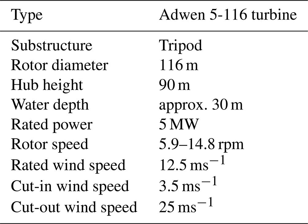
In this work, offshore data from a measurement campaign in the German Alpha Ventus wind farm are utilised. The raw data are freely available for research purposes after signing an agreement concerning the data usage (https://www.rave-offshore.de/en/data.html, last access: 19 September 2022). Alpha Ventus consists of twelve 5 MW turbines: six Senvion 5M turbines mounted on jackets and six Adwen 5-116 turbines mounted on tripods (see Fig. 1). The wind farm is located about 45 km north of the German island Borkum (see Fig. 2). It has water depths of about 30 m.

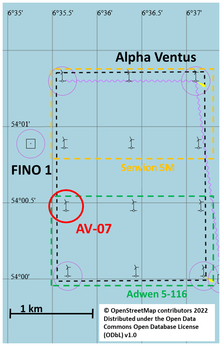
Figure 1 Farm layout of Alpha Ventus with the considered AV-07 turbine marked (adapted from OpenStreetMap).

Figure 2 Location of Alpha Ventus and the met mast FINO1 (adapted from OpenStreetMap).

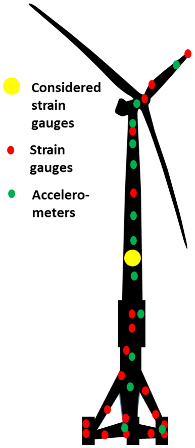
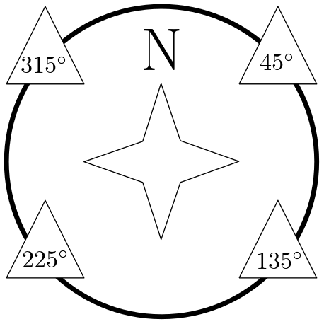
Alpha Ventus was commissioned in April 2010. The measurement campaign started in 2011. Since then, not only have SCADA data been collected, but environmental conditions, strains, accelerations, etc. have also been measured as well. Further environmental data are available from the met mast FINO1 (https://www.fino1.de/en/, last access: 19 September 2022). FINO1 is located next to the Alpha Ventus wind farm (compare Fig. 1). This work focusses on the AV-07 turbine (see Table 1). It is marked in Fig. 1. This turbine is equipped with more than 100 sensors on the rotor–nacelle assembly, the tower, and the substructure above and below sea level. Data concerning environmental conditions are available as statistical values – i.e. mean values, standard deviations, maxima and minima – at 10 min intervals. Strain data are provided as high-resolution (50 Hz) time series for several locations (see Fig. 3). As an example, this work uses the strain data from one location on the tower, as marked in Fig. 3. At this location, four strain gauges are placed around the circumference of the tower (see Fig. 4).

Table 1 Properties of the investigated AV-07 turbine (Bartsch, 2020).

Figure 3 Illustration of the AV-07 turbine (not to scale) and some of the installed sensors according to the sensor documentation (IWES, 2019).

Figure 4 Positions of the strain gauges around the circumference of the tower.

Although measurement data are, in general, available for time periods since 2011, for many periods, the data quality is not sufficient for fatigue damage extrapolations. Many sensors have experienced defects, leading to missing or erroneous data. For fatigue extrapolations, it is important that data are recorded with a high availability for a continuous period of at least 1 year to cover seasonal effects properly. Since data of higher quality are available for the sensors on the tower compared to sensors on the substructure, this work only considers data from the previously mentioned strain gauges on the tower. Moreover, only the data from 3 specific years have a sufficient quality to be taken into account: 1 January to 31 December 2011 and 1 October 2015 to 30 September 2017. For these 3 years, raw data are post-processed as described in the next section before calculating fatigue damage.

2.2 Raw data and data processing

For this work, three types of data are required: strain data, data regarding environmental conditions and data concerning operational conditions.

Strains are measured on the tower of the AV-07 turbine (see Fig. 3). Four temperature-compensated strain gauges are positioned around the circumference of the tower (see Fig. 4). The raw data were post-processed using semi-automatic methods to exclude, for example, erroneous data as shown in Fig. 5. Zero values and unrealistically high and low values are excluded automatically. Some additional values are excluded manually after visual inspections of the data. Profound post-processing and full sensor calibrations were not performed. The reasons for this are, first, in an industry context, time-consuming manual post-processing is prohibitive. Second, due to the long measurement period of approximately 7 years, the identification of all sensor drifts is not straightforward. And lastly and most importantly, it is a common assumption to neglect the mean value of the signals for the fatigue damage calculation (cf. Sect. 3.1). Surely, this assumption is a simplification which could be resolved, for example, by applying a so-called Goodman correction (Goodman, 1914). However, for this work, not taking into account the mean values is a valid assumption. Some example data after the post-processing can be seen in Fig. 6.

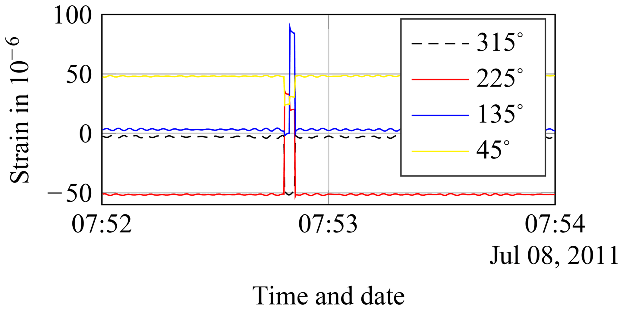
Figure 5 Example strain data before post-processing, which include clearly erroneous measurements, i.e. physically unrealistic peak without any oscillation afterwards.

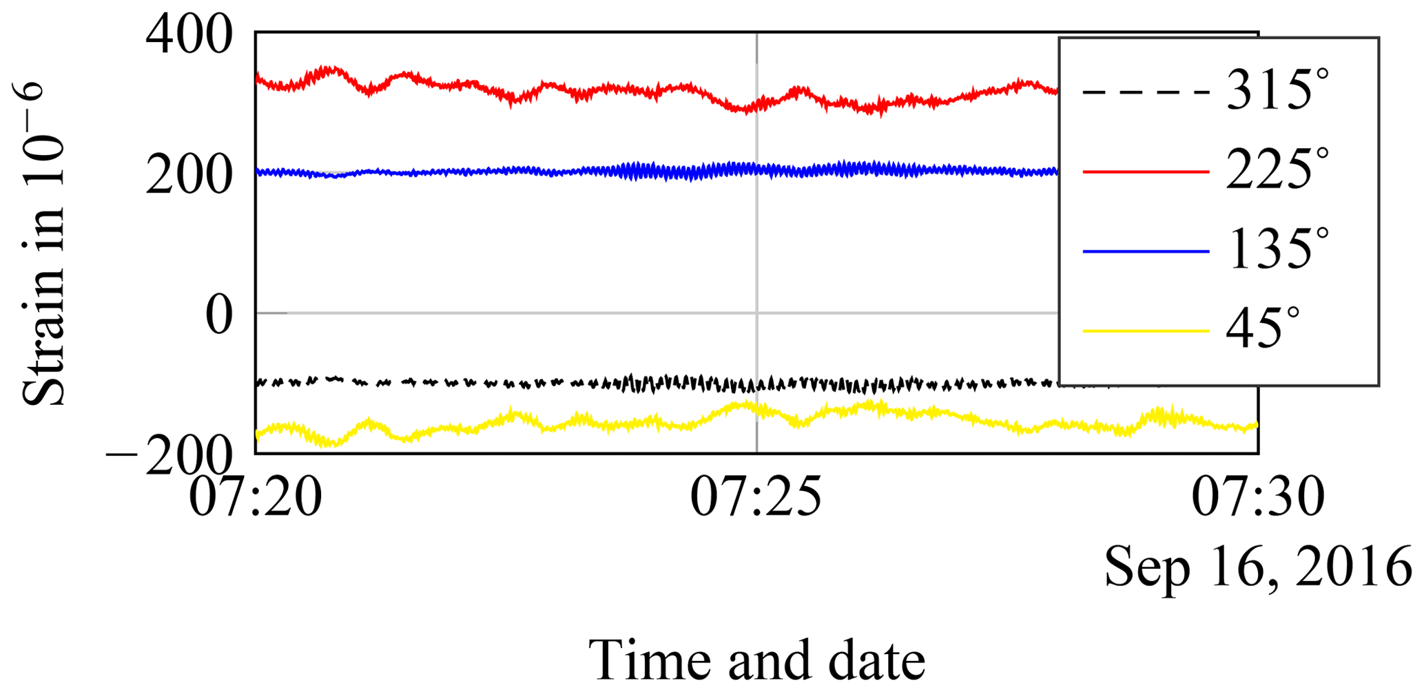
Figure 6 Example strain data. A wind direction of approximately 235^∘ leads to wind-induced oscillations for the sensors at 225^∘ (tension) and 45^∘ (compression) and oscillations in its eigenfrequencies in side-to-side direction (sensors at 135 and 315^∘).

Operational conditions are taken from SCADA data from the AV-07 turbine. Environmental conditions are, in most cases, taken from the FINO1 met mast. Only if no data are available from FINO1, are the wind conditions included in the SCADA data from the AV-07 turbine taken into account. FINO1 data are available for approximately 95 % of all 10 min intervals. Another 3 % of the intervals are filled up using SCADA data, yielding a data availability for the environmental conditions of above 98 %. The reason for using FINO1 data whenever available is that they are of higher quality. There are no or at least fewer disturbance effects, e.g. no increased turbulence or reduced wind speed caused by the rotor. Still, all extrapolation methods applied in this work could also be used if no met mast data, i.e. only SCADA data, are available (see Appendix A for an exemplary comparison of met mast plus SCADA data and pure SCADA data using the example of the binning approach). For this work, six environmental conditions, namely wind speed, wind direction, turbulence intensity, significant wave height, wave peak period and wave direction, are considered. The selection of these six environmental conditions was done based on the available data and results of previous sensitivity analyses, e.g. Hübler et al. (2017). In addition, the turbine status – recorded by the SCADA system, e.g. normal operation, start-up and emergency stop – is taken into account. Classical operational conditions like power output or pitch angle are partly covered by using the turbine status. For all EOCs, only statistical values, e.g. mean values of 10 min intervals, are available. At FINO1, wind conditions are measured at 90 m above mean sea level. The wind speed is measured using cup anemometers. These are positioned on jibs in secondary wind directions to reduce shadow effects. A buoy in the immediate vicinity of FINO1 (about 150 m away) measures the wave conditions. The available EOC data are post-processed using semi-automatic methods. For example, values below and above certain thresholds, and consecutive values that are precisely the same are excluded. As stated before, missing or erroneous data are replaced by SCADA measurements to increase the number of 10 min intervals for which strain and EOC data are available. Some example data after the post-processing can be seen in Fig. 7. Since EOC data are mainly used for the binning (see Sect. 3.2), the slightly biased wind data, due to rotor disturbance when using SCADA data, are less relevant compared to the increase in the overall amount of data. Or, in other words, in this context, the amount of EOC data is more relevant than the EOC data quality. This statement is only correct if the statistical difference between FINO1 and SCADA data is small (here: ${\mathrm{CV}}_{\text{FINO}}={\mathrm{CV}}_{\text{SCADA}}=\mathrm{0.5}$). Moreover, since SCADA data will always feature smaller mean wind speeds (here: μ_FINO=9.3 ms⁻¹ and μ_SCADA=8.3 ms⁻¹), it is also essential to use the same data source for the entire analysis, e.g. not FINO1 data during the measurement period and SCADA data for the extrapolation period.

Figure 7 Example wind speed data after the post-processing.

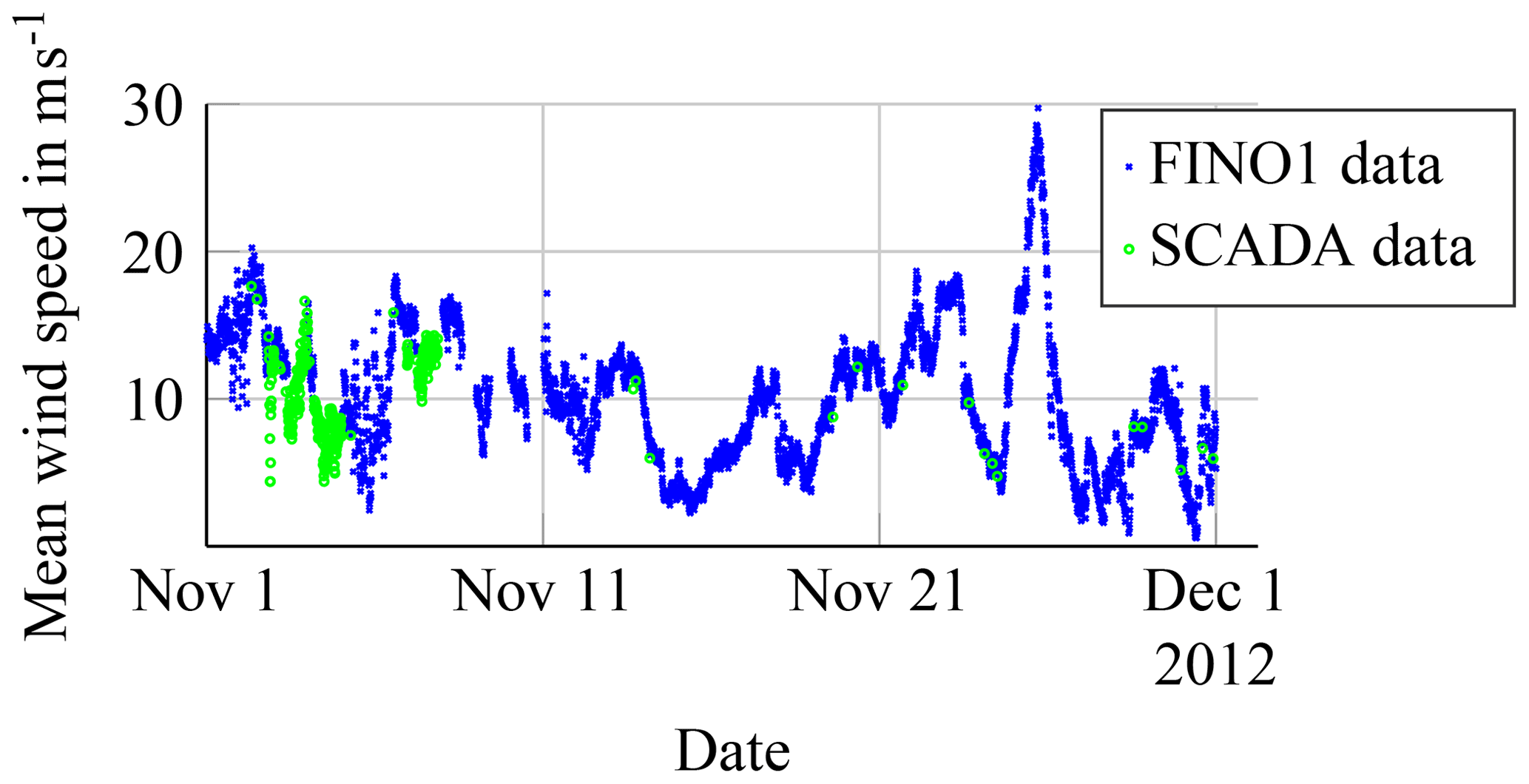
Figure 8 Correlation of wind speeds and logarithmised short-term damage values (D_j) determined using the strain gauge at 315^∘. Histogram based on all 10 min intervals in 2016.

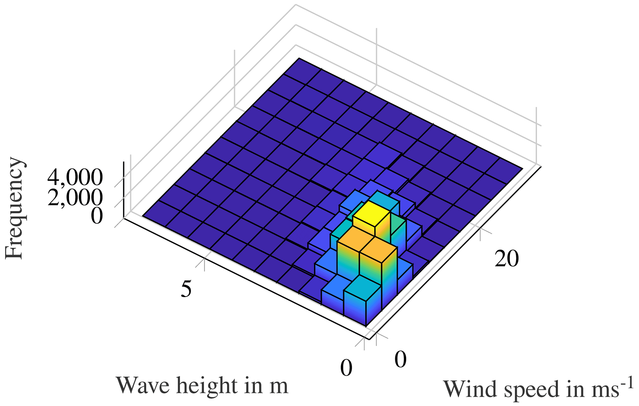
Figure 9 Correlation of wind speeds and wave heights. Histogram based on mean values of all 10 min intervals in 2016.

As stated in the Introduction, most extrapolation approaches are based somehow on correlations between fatigue damage and EOCs. This correlation is shown as an example in Fig. 8 for the wind speed and a short-term damage to the tower. There is a pronounced correlation for all wind speeds. For high wind speeds, it is more visible, since the amount of data is lower for high wind speeds. As EOCs are also correlated with each other – as shown in Fig. 9 – it is not straightforward to determine the relevant EOCs that need to be considered for the extrapolation in time. Before discussing different approaches for extrapolation in time in Sect. 3.2, in the next section, some more information on the short-term fatigue damage calculation is given.

In the following, a 10 min interval is only considered if strain and complete EOC data are available.

3 Fatigue damage calculation

Assuming a linear damage accumulation according to the Palmgren–Miner rule, the overall damage, e.g. the lifetime damage of a structure, can be calculated as the sum of many short-term damage values. It is known that linear damage accumulation is a simplification of the real fatigue behaviour. For example, sequence effects are neglected. Moreover, the use of short-term intervals, e.g. 10 min intervals, for the damage calculation is a simplification as well. In this case, long-term fatigue cycles lasting several hours or even days are not taken into account (Marsh et al., 2016; Sadeghi et al., 2022). Still, this procedure is recommended for the design of offshore steel structures (DNVGL, 2014), since it leads to relatively small errors for steel components compared to its use in the context of composite materials, for example, in rotor blades. Based on this assumption, for each 10 min interval, the (short-term) fatigue damage is calculated separately. The calculation procedure for the short-term damage based on strain measurements is fairly standardised and is briefly presented in the following section. It should be noted that this work focusses on the damage at a single location (cf. Fig. 3). Most results are given for the strain gauge at 315^∘ being a strain gauge which is positioned approximately perpendicular to the dominant wind direction. A spatial interpolation between the four strain gauges to determine a maximum around the circumference or to calculated stress time series for various points around the circumference is not done. Such a spatial interpolation would be needed to actually determine the fatigue life of the turbine in an industrial context. Similarly, if fatigue damage values at other locations are required, either data from additional strain gauges must be used or spatial extrapolations (Maes et al., 2016; Henkel et al., 2020) are needed. Still, for the current purpose, i.e. to assess and validate methods for extrapolations in time, it is reasonable to use a single strain gauge.

3.1 Short-term damage

Assuming linear damage accumulation and a fixed location at which high-resolution strain data (ϵ(t)) are available, the fatigue damage sustained in a given time period can be calculated as follows. First, stress time series (σ(t)) are determined by applying Hooke's law,

$$\begin{array}{}\text{(1)}& \mathit{\sigma }\left(t\right)=E\mathit{ϵ}\left(t\right),\end{array}$$

where E is Young's modulus. Since it is assumed that strain data are already available for the required location, e.g. height and position around the circumference of the tower, a rain flow cycle counting of stress ranges (Δσ_i) can be applied directly to the stress time series. Here, Δσ_i is the stress range of the ith band (also called block or bin) in the factored stress spectrum (cf. Annex A of European Committee for Standardization, 2010). In this work, a cycle counting according to Niesłony (2009) is applied. The number of required stress bands (n_σ) is chosen to be 500 bands – logarithmically spaced between 10 kPa and 1 GPa (Hübler et al., 2019). Two example cycle counts for a 10 min interval are shown in Figs. 10 and 11. Figure 10 shows the cycle count for a strain gauge in the fore-aft direction, and Fig. 11 shows one in the side-to-side direction. The latter clearly features many cycles corresponding to the eigenfrequency of the structure (peak just above 10⁶ Pa).

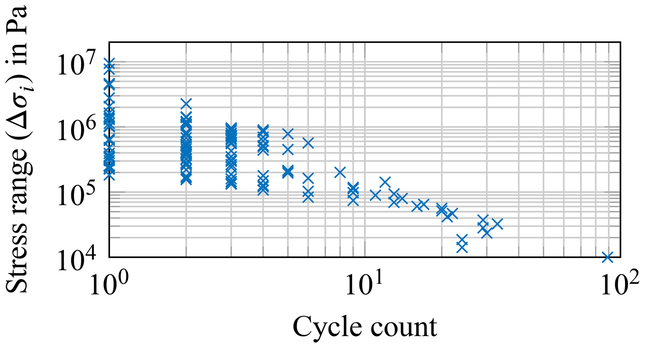
Figure 10 Results of the rain flow cycle count for a 10 min interval (18 March 2016; 00:10:00). Strain gauge at 315^∘, which corresponds to fore-aft direction for this interval.

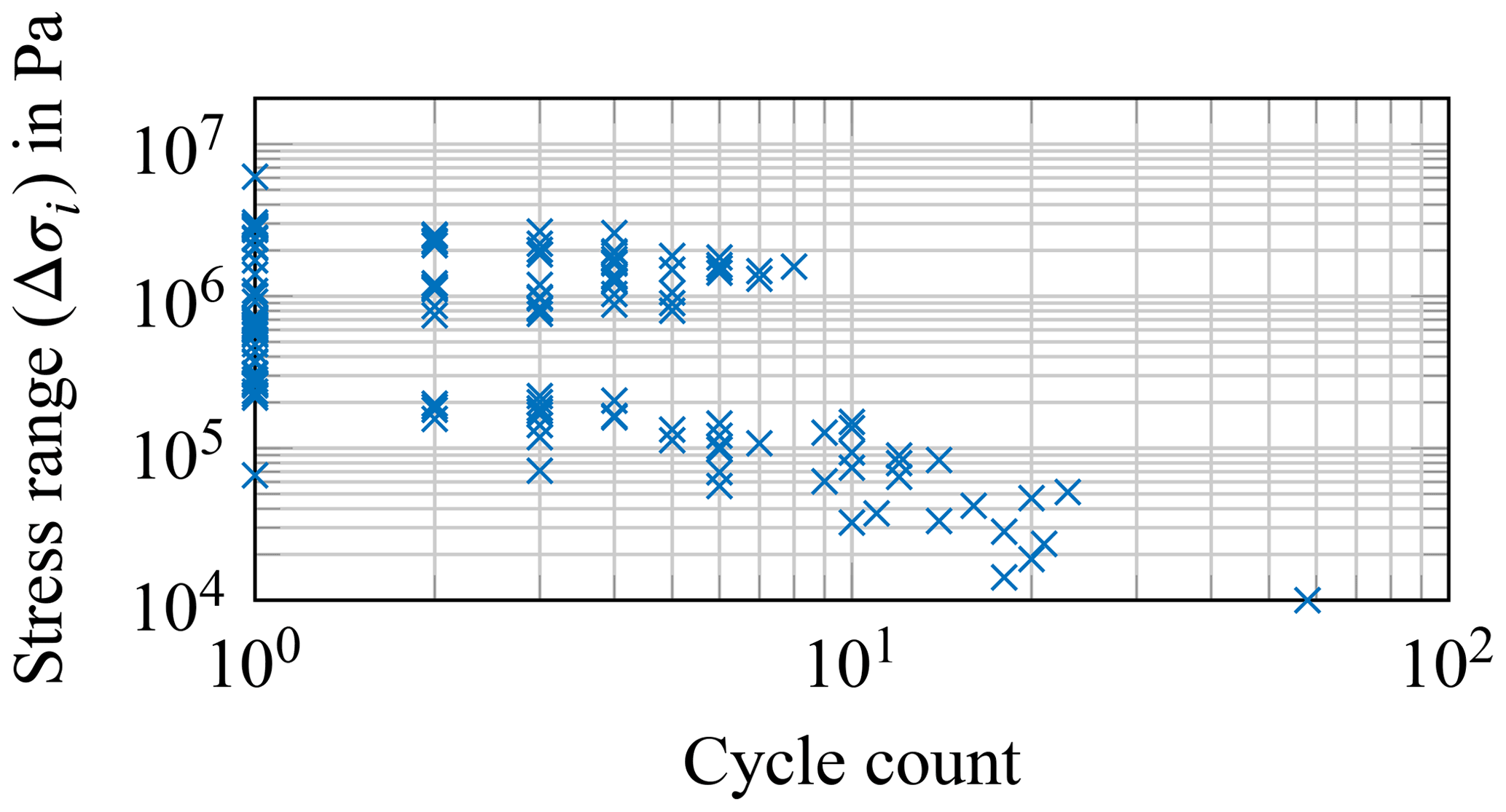
Figure 11 Results of the rain flow cycle count for a 10 min interval (18 March 2016; 00:10:00). Strain gauge at 225^∘, which corresponds to side-to-side direction for this interval.

For nominal stresses at the position of interest (here: the measurement position), an overall safety factor (SF) is applied. It consists of several sub-factors. Using the safety factor, a representative value for the concentrated stresses at the structural detail is achieved. First, a stress concentration factor for the specific detail is used (here: SCF =1.0 according to a recommended practice of DNVGL, 2014). Second, a correction for large wall thicknesses – the so-called size effect (SE) correction – is applied (DNVGL, 2014). Third, a material safety factor (here: MSF =1.0 due to regular inspections, DNV GL AS, 2016) is used. All these factors might be chosen differently and/or can be regarded as uncertain. For example, the stress concentration factor highly depends on the exact detail. Depending on whether the welding is single or double sided, how large the ovality and/or eccentricity of the two connected parts of the tower are or the precise thickness of the tower at this position, SCF =1 to SCF =2, are equally possible. Surely, such variations in the SCF have significant influence on the short-term fatigue. Moreover, in reality, safety factors also depend on the inspection and monitoring concepts used. For example, it might be possible to reduce safety factors if monitoring-based approaches – as presented in this work – are applied. Hence, determining adequate safety factors and, therefore, calculating precise short-term damage values is not trivial, especially if not all structural details of the turbine are available. Fortunately, to assess the extrapolation in time, precise values for the safety factor are not required. The corrected stress ranges can be calculated as follows:

$$\begin{array}{}\text{(2)}& \mathrm{\Delta }{\mathit{\sigma }}_{\mathrm{cor},i}=\mathrm{\Delta }{\mathit{\sigma }}_i\times \mathrm{SF}=\mathrm{\Delta }{\mathit{\sigma }}_i\times \mathrm{SCF}\times \mathrm{SE}\times \mathrm{MSF}.\end{array}$$

The last step in calculating the damage sustained in a given interval is the application of the Palmgren–Miner rule, i.e. linear damage accumulation, and the application of S–N curves according to the DNVGL recommended practice (DNVGL, 2014). Here, DNVGL S–N curve D in air is applied. At this point, it should be noted that this S–N curve consists of two parts with different slopes but does not account for a fatigue limit in the material, i.e. no horizontal part at low stress cycles. The “missing” fatigue limit might lead to an overestimation of the influence of small cycles. However, since the determination of most suitable S–N curves is out of the scope of this work, here, the S–N curve as given in the DNVGL recommended practice (DNVGL, 2014) is used. The fatigue damage for a given time series (D_j) can be calculated as follows:

$$\begin{array}{}\text{(3)}& D_j=\sum _{i=\mathrm{1}}^{n_{\mathit{\sigma }}}{\displaystyle \frac{n_{ij}}{N_i}},\end{array}$$

where i and j are indices for the stress band and the time series, respectively, and n_ij is the number of cycles associated with the stress range Δσ_cor,ij. The endurance (N_i; maximum number of cycles) for the same stress range is obtained from the corresponding S–N curve.

3.2 Damage extrapolation in time

If strain data were available for the entire lifetime of the wind turbine, it would be possible to determine its fatigue lifetime by using the previously described approach of calculating short-term damage values. In this case, the lifetime damage (D_total) would be

$$\begin{array}{}\text{(4)}& D_{\text{total}}=\sum _{j=\mathrm{1}}^{N_{\text{LT}}}{D}_j,\end{array}$$

where N_LT is the number of (short-term) intervals in the entire lifetime, e.g. $N_{\text{LT}}=\mathrm{6}\times \mathrm{24}\times \mathrm{365.25}\times \mathrm{20}$ for 10 min intervals and a lifetime of 20 years.

However, normally, strain data are not available for the entire lifetime. Therefore, some kind of extrapolation procedure in time is necessary. In the following, three different approaches are presented: a simple linear extrapolation, an extrapolation based on bins of EOCs and an extrapolation based on machine-learning techniques. The latter two make use of the correlation of short-term damage and EOCs (cf. Fig.  8).

In a real application, new data might come in continuously or discontinuously after having conducted a first extrapolation. Hence, updates of the extrapolation using additional data have to be possible. For all three approaches, such updates are feasible. Since the computing times of the approaches are relatively low in order to enable uncertainty assessments (cf. Sect. 3.2.4), discontinuous updates can be achieved by rerunning the entire extrapolation. For continuously incoming data, a simplification could be to update the occurrence probability of the EOCs continuously and the correlation itself on a discontinuous basis, e.g. once a month.

3.2.1 Simple extrapolation

The simplest extrapolation approach is a linear extrapolation. It assumes that the fatigue damage only depends on the elapsed time (Louraux and Brühwiler, 2016). This means that the fatigue damage sustained in any predicted period can be calculated as follows:

$$\begin{array}{}\text{(5)}& D_{\text{pred}}\approx {\displaystyle \frac{N_{\text{n}}}{N_{\text{m}}}}\sum _{j=\mathrm{1}}^{N_{\text{m}}}{D}_j,\end{array}$$

where N_m and N_n are the number of (short-term) intervals in the measurement and the predicted period, respectively. If the predicted period is the entire lifetime, it follows that

$$\begin{array}{}\text{(6)}& D_{\text{total}}\approx {\displaystyle \frac{N_{\text{LT}}}{N_{\text{m}}}}\sum _{j=\mathrm{1}}^{N_{\text{m}}}{D}_j.\end{array}$$

For very long measurement periods (N_m≈N_LT), this approach yields accurate results. However, if the measurement period is less than 1 year, seasonal effects are neglected. For example, storms during the winter lead to increased damage. Even if the measurement period covers more than a year, yearly and/or long-term effects are not taken into account, e.g. varying damage due to climate change (Hübler and Rolfes, 2021).

3.2.2 Extrapolation based on bins of EOCs

A more advanced approach, which makes use of the correlation between fatigue damage and EOCs (cf. Fig. 8), is a so-called binning approach (Marsh, 2016; Hübler et al., 2018). This binning approach is still very simple to apply and, therefore, quite user-friendly. The binning approach is based on the idea that most variations in fatigue damage are due to changing environmental conditions. Hence, it is not necessary to know fatigue damage for the entire lifetime. Having determined the correlation between EOCs and fatigue damage, it is sufficient to know the EOCs for the entire lifetime. Since many EOCs are part of the SCADA data, EOCs are frequently known for the entire lifetime. Hence, the only challenge is determining the correlation between fatigue damage and EOCs. This correlation can be determined by statistical and/or machine-learning techniques (Dimitrov and Natarajan, 2019; d N Santos et al., 2021) that yield a functional relationship between (short-term) damage and EOCs:

$$\begin{array}{}\text{(7)}& D_j=f\left({\mathbf{x}}_j\right)+\mathit{ϵ},\end{array}$$

where f is the functional relationship; x_j is the vector of all EOCs considered in the analysed interval j; and ϵ is an error term, which cannot be explained by changes in the EOCs considered. Such functional relationships are discussed in the next section. The binning approach presumes that, due to the uncertainty in the measured EOCs (e.g. disturbance of the wind conditions by the rotor) and some unexplained variations in the fatigue damage (ϵ), a precise definition of a function is not expedient. Therefore, the (short-term) damage values are clustered according to the EOCs. For each cluster or bin, the mean damage is determined using the available measured strain data. The calculation of mean values is supposed to average out most unexplained effects (ϵ). Subsequently, the damage sustained in the predicted period is

$$\begin{array}{}\text{(8)}& D_{\text{pred}}\approx N_{\text{n}}\sum _{i_{\mathrm{1}}=\mathrm{1}}^{M_{\mathrm{1}}}\mathrm{\dots }\sum _{i_d=\mathrm{1}}^{M_d}\left(P{r}_{\text{pred},i_{\mathrm{1}},\mathrm{\dots },i_d}{\stackrel{\mathrm{‾}}{D}}_{i_{\mathrm{1}},\mathrm{\dots },i_d}\right),\end{array}$$

where d is the binning dimension, i.e. the number of EOCs considered; M₁ to M_d are the number of bins for the corresponding EOC; and $P{r}_{\text{pred},i_{\mathrm{1}},\mathrm{\dots },i_d}$ and ${\stackrel{\mathrm{‾}}{D}}_{i_{\mathrm{1}},\mathrm{\dots },i_d}$ are the occurrence probability of and the mean damage in bin $i_{\mathrm{1}},\mathrm{\dots },i_d$, respectively. Mean damage within the bins can be determined using a limited amount of strain data, e.g. 1 year (measurement period). To determine the bin probabilities, only data concerning the EOCs are required. Hence, bin probabilities are determined using data of the predicted period. If the predicted period is the entire lifetime, it follows that

$$\begin{array}{}\text{(9)}& D_{\text{total}}\approx N_{\text{LT}}\sum _{i_{\mathrm{1}}=\mathrm{1}}^{M_{\mathrm{1}}}\mathrm{\dots }\sum _{i_d=\mathrm{1}}^{M_d}\left(P{r}_{\text{LT},i_{\mathrm{1}},\mathrm{\dots },i_d}{\stackrel{\mathrm{‾}}{D}}_{i_{\mathrm{1}},\mathrm{\dots },i_d}\right).\end{array}$$

The main difference is that bin probabilities ($P{r}_{\text{LT},i_{\mathrm{1}},\mathrm{\dots },i_d}$) are now determined using EOC data, e.g. SCADA data, covering the entire lifetime. In contrast to the previously presented simple extrapolation, seasonal effects and long-term changes due to changing EOCs are taken into account by the bin probabilities. The main challenge of the binning approach is to apply expedient binning dimensions and bin numbers. Too few bins – i.e. a low number of bins per dimension and/or a low dimensionality – result in highly scattered damage values within each bin. This yields a less accurate approximation of the correlation. In the extreme case of d=0, the binning approach is identical to the simple extrapolation. Too many bins lead to only a few short-term damage values within each bin or even empty bins. These empty or nearly empty bins have to be filled up. For 1D binning, in most cases, no bins have to be filled up. However, for 2D bins, it is already necessary to fill up about 40 % of the bins (cf. Fig. 9). Most of the empty bins feature very low occurrence probabilities and, therefore, do not influence the overall fatigue damage. Nonetheless, if the fatigue extrapolation is based on fairly limited data, the filling of empty bins may lead to biased results. In this work, only bins with no data at all are considered to be empty. These empty bins are filled up relatively conservatively. The largest mean value of the surrounding bins is used. Hence, the mean damage in bin $i_{\mathrm{1}},\mathrm{\dots },i_d$ can be calculated as follows:

$$\begin{array}{}\text{(10)}& {\stackrel{\mathrm{‾}}{D}}_{i_{\mathrm{1}},\mathrm{\dots },i_d}=\left\{\begin{array}{ll}\frac{\mathrm{1}}{N_{i_{\mathrm{1}},\mathrm{\dots },i_d}}{\sum }_{j=\mathrm{1}}^{N_{i_{\mathrm{1}},\mathrm{\dots },i_d}}{D}_j& \text{if }{N}_{i_{\mathrm{1}},\mathrm{\dots },i_d}>\mathrm{0}\\ max\left({\stackrel{\mathrm{‾}}{D}}_{i_{\mathrm{1}}+j_{\mathrm{1}},\mathrm{\dots },i_d+j_d}\right)& \text{otherwise},\end{array}\right.\end{array}$$

where $N_{i_{\mathrm{1}},\mathrm{\dots },i_d}$ is the number of short-term damage values in bin $i_{\mathrm{1}},\mathrm{\dots },i_d$ and $j_k=\mathit{\{}-\mathrm{1},\mathrm{0},\mathrm{1}\mathit{\}}$ if $\mathrm{1}<i_k<M_k$, $j_k=\mathit{\{}\mathrm{0},\mathrm{1}\mathit{\}}$ if i_k=1 and $j_k=\mathit{\{}-\mathrm{1},\mathrm{0}\mathit{\}}$ if i_k=M_k for $k=\mathrm{1},\mathrm{\dots },d$.

3.2.3 Extrapolation based on a functional relationship

As already discussed in the previous section, the correlation between short-term damage and EOCs can also be expressed as a functional relationship, i.e. $D_j=f\left({\mathbf{x}}_j\right)+\mathit{ϵ}$. In general, such a functional relationship can be approximated using various statistical and/or machine-learning techniques, e.g. multiple regression, Gaussian process regression (GPR) and artificial neural networks (ANNs). To determine the functional relationship, training data are required to train the relation between inputs, i.e. EOCs, and outputs, i.e. fatigue damage values. Similar to the binning approach, it is not necessary for strain data to be available for the predicted period or the entire lifetime. The strain and EOC data from the measurement period, e.g. 1 year, are used as training data. Subsequently, fatigue damage for other time periods can be predicted using EOC data only. EOC data are normally available for the entire lifetime.

$$\begin{array}{}\text{(11)}& {\displaystyle }{D}_{\text{pred}}& {\displaystyle }\approx \sum _{k=\mathrm{1}}^{N_n}f\left({\mathbf{x}}_k\right)\text{and}\text{(12)}& {\displaystyle }{D}_{\text{total}}& {\displaystyle }\approx \sum _{k=\mathrm{1}}^{N_{\text{LT}}}f\left({\mathbf{x}}_k\right)\end{array}$$

The accuracy of the prediction also depends on the EOCs considered. If too few EOCs are taken into account, important features might be missed. Too many EOCs might lead to some kind of overfitting.

In this work, GPR and ANN are investigated. Both methods are very powerful machine-learning techniques which have already been applied successfully in wind engineering (Dimitrov et al., 2018; d N Santos et al., 2021). On the downside, they are less user-friendly compared to the binning approach. At least some expert knowledge is required to achieve accurate predictions.

All configurations for ANN and GPR used in this work are based on recommendations in literature, e.g. Larose and Larose (2014); previous work, e.g. Müller et al. (2021); and preliminary studies.

For ANN, inputs and outputs are normalised to values between 0 and 1. Two hidden layers with 10 neurons each are used. Hyperbolic tangent sigmoid transfer functions are applied in all layers to prevent unrealistic negative outputs, i.e. negative damage values. The network is trained using the Levenberg–Marquardt algorithm; 80 % of the input data are used as training data, and 20 % are used as validation data. Since the performance of ANN depends strongly on the randomly chosen initial weights for this problem, an automated control algorithm is implemented. It restarts the learning process using new initial weights if the relative prediction error is higher than 50 % for the training data.

For GPR, inputs are normalised to values between 0 and 1. Outputs are standardised to achieve a mean value of 0 and a standard deviation of 1. A purely quadratic basis function and a Matérn kernel with a parameter of $\mathrm{5}/\mathrm{2}$ and a separate length scale per input are chosen. Since the amount of training data is extensive, e.g. more than 50 000 training data points from 1 year of measurements, a random subset selection for the training is conducted. This reduces the time required for training the model to a practicable level. Since ANN and GPR both feature some random effects themselves (initial weights and selected subsets), a statistical evaluation of both is beneficial. Hence, the functional relationship f(x) should be trained several, e.g. 100, times using the same training data. This averages out the effect of the inherent randomness, i.e. the model uncertainty. The averaging technique for ANN and GPR is discussed in more detail in Sect. 4.2.

3.2.4 Uncertainty assessment

Independent of the chosen extrapolation approach, the results will be uncertain, for example, due to unrepresented EOCs. Nonetheless, the main reason for this uncertainty is the limited amount of strain data and, therefore, of short-term damage values (D_j). This uncertainty due to limited training data should not be confused with the model uncertainty mentioned in the previous section which is only relevant for ANN and GPR. To approximate the uncertainty of the predicted (D_pred) or overall fatigue damage (D_total) due to limited data, bootstrapping (Efron, 1979) can be applied (Marsh, 2016). Bootstrapping allows for the estimation of a distribution of D_pred or D_total by applying random sampling with replacement. This distribution can be used to judge the uncertainty present. For example, the standard deviation or percentile values of this distribution are relevant measures of uncertainty.

In the present case, short-term damage values (D_j) are limited – e.g. only available from 1 year of strain measurements. Hence, using another year of measurement data yields a (slightly) different correlation between EOCs and damage values; i.e. f(x_k) or ${\stackrel{\mathrm{‾}}{D}}_{i_{\mathrm{1}},\mathrm{\dots },i_d}$ is different. As a consequence, D_pred or D_total change as well. However, other values for D_j are not available. Therefore, D_pred or D_total is calculated several times using different samples D_j, which are sampled randomly with replacement from all available samples {D₁,…$,D_{N_m}\mathit{\}}$. As an illustration, for N_m=3, the standard calculation would be based on the samples $\mathit{\{}{D}_{\mathrm{1}},D_{\mathrm{2}},D_{\mathrm{3}}\mathit{\}}$. Other random realisations with replacement are, for example, $\mathit{\{}{D}_{\mathrm{1}},D_{\mathrm{1}},D_{\mathrm{1}}\mathit{\}}$ or $\mathit{\{}{D}_{\mathrm{2}},D_{\mathrm{2}},D_{\mathrm{3}}\mathit{\}}$. For each realisation (i.e. new training data set), the entire extrapolation procedure described in Sect. 3.2 has to be repeated; e.g. a new correlation f(x_k) has to be determined.

4 Results

In this section, the three methods for the temporal extrapolation of fatigue damage, which were presented in the previous section, are assessed using measurement data from the Alpha Ventus wind farm (see Sect. 2). The assessment tries to answer the subsequent questions:

1. How should the parameters of each of the methods, e.g. bin sizes, be chosen to yield the most accurate results?

2. Which method can predict fatigue damage for other time periods most accurately?

3. How high is the uncertainty in the prediction?

4. What amount of training data is required? How long is the minimum measurement period?

5. Do the approaches still yield reasonable results if long-term extrapolations over several years are conducted?

6. Do the approaches still yield reasonable results if extrapolations into the future are conducted, for which no EOC data are available?

Since high-quality strain data are only available for 3 years, for most steps, an extrapolation of measurement data from a single year to another year is conducted. For example, data from October 2015 to September 2016 are extrapolated to October 2016 to September 2017. Since strain and EOC data are available for both periods, the accuracy of the extrapolation can be determined by comparing the predicted damage (D_pred) with the damage calculated using the actual measured strain data from the predicted period, i.e. the real damage (D_real). Hence, the methods can be validated.

4.1 Parameter selection

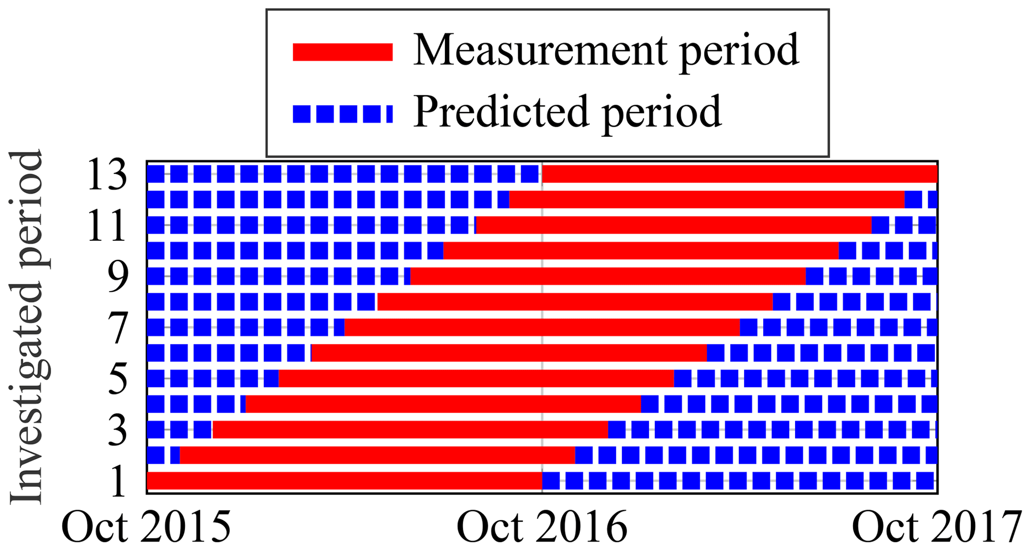
For the three extrapolation methods considered in this work, different parameters must be chosen, for example, the number of EOCs to be taken into account. To determine the most suitable parameters, the extrapolation from a single year to another year is analysed. Since the choice of the parameters might be influenced by the period investigated, several periods should be analysed. However, only 3 years of data is available, with only 2 of these being consecutive years. For the third, non-consecutive year (2011), long-term effects – being analysed in Sect. 4.5 in detail – might already be relevant. Hence, within the 2 consecutive years, the 1-year period is shifted, e.g. with October 2015 to September 2016 being extrapolated to October 2016 to September 2017, November 2015 to October 2016 being extrapolated to October 2015 and November 2016 to September 2017. A visualisation of this shifting procedure is shown in Fig. 12. Using these shifted periods, 13 “different” periods are available. Therefore, some statistical significance for the determined parameters is given.

Figure 12 Visualisation of the 13 different 1-year periods for statistical evaluations.

4.1.1 Parameter selection: simple extrapolation

For the simple extrapolation, no parameters have to be chosen. First results for the simple extrapolation are presented in Fig. 13. For all 13 periods of 1 year, the unsigned percentage errors (PEs) of the predicted yearly damage are shown as follows:

$$\begin{array}{}\text{(13)}& \mathrm{PE}={\displaystyle \frac{|D_{\text{real}}-D_{\text{pred}}|}{D_{\text{real}}}}.\end{array}$$

Moreover, a box plot shows some summary statistics: the median (red centre line), the 25th and 75th percentile (box), the minimum and maximum values (excluding any outliers), and possible outliers of 13 different 1-year measurement periods. Hence, the box plots visualise the variation in the accuracy of the predictions depending on the period considered. All box plots in the following sections show the same summary statistics. To judge the conservatism of the approach, signed errors are more informative. For such results, the reader is referred to Sect. 4.3.

Figure 13 Percentage errors of predicted yearly damage values using a simple extrapolation method compared to real yearly damage values. Prediction from a year to a second year for 13 different years. Box plot shows summary statistics.

Clearly, the prediction does not yield precise results. Nonetheless, it is remarkable that even such a simple extrapolation leads to results with errors of less than 35 %.

4.1.2 Parameter selection: EOC bins

For the extrapolation based on bins of EOCs, the number and type of EOCs to be taken into account and the bin size must be selected. In contrast to previous work by Louraux and Brühwiler (2016) and Hübler et al. (2018), who focussed on one to three different wind parameters, in this work, six different environmental conditions (wind speed and direction, turbulence intensity and wave height, period and direction) are analysed in a systematic manner. Bin sizes are chosen in such a way that the overall range of each environmental condition is discretised into about 3 to 120 bins depending on the environmental condition. For example, bins of 0.25 to 6 ms⁻¹ are used for the wind speed. Regarding operational conditions, only the turbine status is considered. As bin sizes for the turbine status (a discontinuous variable) have to be defined differently, operational conditions are considered separately in a second step (see Sect. 4.1.4).

Some example results for the binning approach are presented in Fig. 14. As before, the box plot shows summary statistics of 13 different measurement periods. On the one hand, the results clarify that many bin types yield similar results. The detailed performance depends on the time period considered, i.e. the year in this case, as demonstrated by the scatter illustrated by the box plot. On average (cf. red centre lines of the box plots), it does not make a significant difference whether, for example, wind speed bins or wind speed and turbulence intensity bins are used. Most important is the consideration of the wind speed. This result is in accordance with previous research (Hübler et al., 2018). On the other hand, the results also demonstrate that there are bin types that perform worse. For example, wind direction and turbulence intensity bins without considering the wind speed or 6D bins do not perform very well. If the wind speed is neglected, important effects are missed. If the binning dimension is too high, a large number of bins remain empty. Hence, the empty bins have to be filled up artificially, leading to less accurate extrapolations. Moreover, a high dimensionality leads to increased computing times, which is problematic at least for the uncertainty assessment (cf. Sect. 4.3). The bin size does not have a pronounced effect, as shown in Fig. 14 using the example of 1D bins, i.e. ${\text{1D}}_{v_{\mathrm{s}}}^{\mathrm{6}}$ to ${\text{1D}}_{v_{\mathrm{s}}}^{\mathrm{120}}$. Medium-sized bins (e.g. 10 bins per environmental condition) are recommended. Again, small bin sizes might result in many empty bins. Excessively large bin sizes lead to higher uncertainties within each bin.

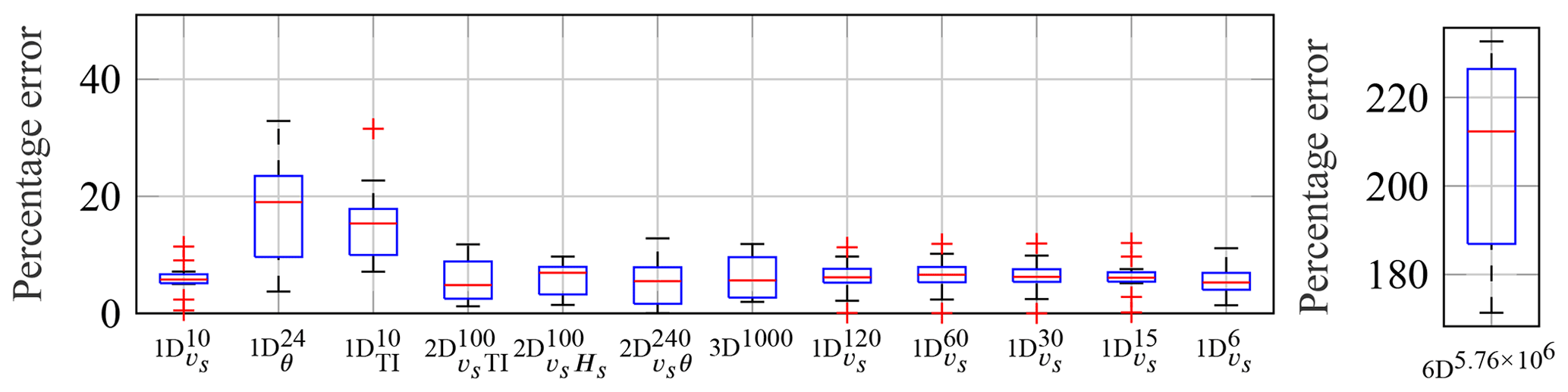
Figure 14 Percentage errors of predicted yearly damage values using a binning method compared to real yearly damage values. Comparison of various bin types and sizes (n is the overall number of bins): wind speed (v_s), wind direction (θ) and turbulence intensity (TI) only (${\text{1D}}_x^n$); combinations of two environmental conditions out of wave height (H_s), v_s, θ and TI (${\text{2D}}_{xy}^n$); v_s, TI and H_s (3D); and all six environmental conditions (6D). Please note: for the sake of clarity, the vertical axis is scaled differently for 6D.

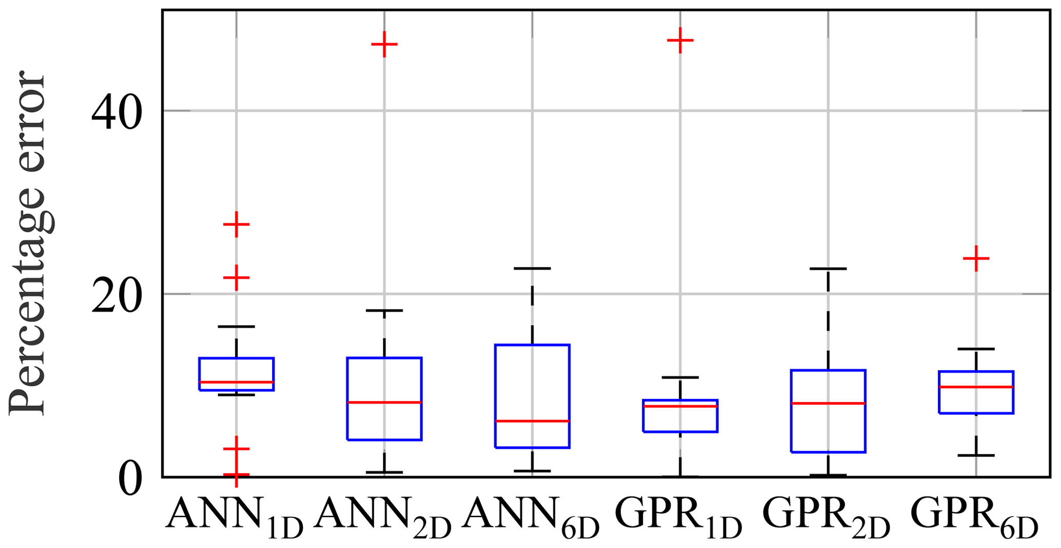
Figure 15 Percentage errors of predicted yearly damage values using a functional relationship compared to real yearly damage values. Comparison of GPR and ANN and different EOCs: v_s (1D), v_s and TI (2D), and all environmental conditions (6D).

The optimal choice always depends on the turbine considered, the measurement period and the extrapolation period. Hence, an automated selection method would be beneficial. Ideally, different choices would be assessed automatically for the predicted period and the best choice selected. However, strain data from the predicted period are normally not available; otherwise no extrapolation would be required. This is why automated selection must be based on cross-validation, i.e. splitting up the measurement period. One part of the data is used as training data to determine the mean damage in all bins. Another part replaces the prediction period. It is used to evaluate the accuracy of the extrapolation for the chosen settings. This procedure reduces the amount of training data significantly. As a result, predictions become less accurate. In most cases, due to the limited training data, the automated selection yields bin sizes which are too fine, i.e. overfitting. Hence, although automated selection is desirable, it is not suitable for “short” measurement periods. For example, measurement periods of 1 year or less – as used in this work – are not sufficient.

Therefore, it can be summarised that the choice of the bin dimension and size is of minor importance as long as empty bins do not occur at all or only in some rare cases. For most applications, simple wind speed bins with a size of 2 to 3 ms⁻¹ are adequate, although they are not optimal. Moreover, fortunately, it is not necessary to take wave conditions into account; these are rarely available, as they are not recorded by the SCADA system. It should be noted that, to some extent, these conclusions might be limited to this turbine and the considered location at the turbine. For example, normally, wave loads become more relevant for larger monopiles and locations further down the turbine. These limitations are discussed in detail in Sect. 5.

4.1.3 Parameter selection: functional relationship

For the extrapolation based on a functional relationship, only the number and type of EOCs to be taken into account are relevant. The same six environmental conditions as before are considered. Operational conditions are taken into account separately in a second step. Some example results for the functional relationship are presented in Fig. 15. Again, the detailed performance depends significantly on the measurement period (cf. scatter shown by the box plots). Moreover, a significant amount of uncertainty is introduced by the random selection of the initial weight using ANN and by the random subset selection using GPR. This is discussed in more detail in Sect. 4.2.

A slight improvement in the accuracy might be achieved for ANN if additional environmental conditions are taken into account. However, this improvement is not significant, especially when considering the previously mentioned uncertainty due to the random selection of the initial weights. At least for wave conditions, it definitely does not justify the effort needed to measure them.

Therefore, in the following, only results using a single environmental condition, i.e. the wind speed, are shown.

4.1.4 Operational conditions

In contrast to the environmental conditions, the turbine status, i.e. the sole considered operational condition, is not defined continuously. This makes the definition of a functional relationship complicated. Hence, in this work, the turbine status is treated differently from the environmental conditions. For all three methods, in a first step, all data are split up according to the turbine status. This means that some kind of binning based on the turbine status is applied for all three approaches. This has the advantage that in each turbine status bin, the extrapolation approach remains unchanged. Finally, the extrapolation results of each turbine status bin are weighted according to the occurrence probability of this turbine status. For the simple extrapolation this yields the following:

$$\begin{array}{}\text{(14)}& D_{\text{pred}}\approx N_{\text{n}}\sum _{k=\mathrm{1}}^K\left({\displaystyle \frac{P{r}_k}{N_{\text{m},k}}}\sum _{j=\mathrm{1}}^{N_{\text{m},k}}{D}_j\right),\end{array}$$

where K is the number of different turbine statuses considered; N_m,k is the number of available short-term damage values for this turbine status; and Pr_k is the occurrence probability of this turbine status, determined using data from the predicted period (e.g. the entire lifetime). For the extrapolation based on a functional relationship, the procedure is equivalent. Hence, a functional relationship f_k(v_s) is trained for each turbine status considered. For the binning approach, it means that just another binning dimension is added. This yields 2D bins: wind speed and turbine status.

Similar to the challenge of determining a suitable bin size, an adequate number of different turbine statuses and the type of statuses must be found. The most simple differentiation is normal production operation and others (two statuses). This was already proposed by Hübler et al. (2018). Other possible classifications are, for example, “normal production operation”, “idling (below cut-in)”, “idling (above cut-off)”, “others” (four statuses) or another additional class for “service” (five statuses). Other combinations of these classes are possible as well but are not investigated in detail in this work. Figures 16 to 18 show how the performance of the three methods changes if operational conditions are taken into account. For all three methods, the effects are not very pronounced and relatively uncertain, i.e. depending on the period considered (cf. scatter shown by the box plot). Nonetheless, percentage errors can be reduced by about 20 % to 30 % for the binning approach and ANN (cf. red centre lines of the box plots) if several different turbines statuses are considered separately. For the simple approach, splitting up the data does not improve the approximation significantly. It should be noted that conclusions regarding the relevance of considering different turbine statuses are at least partly case-specific. This limitation is discussed in Sect. 5 in more detail.

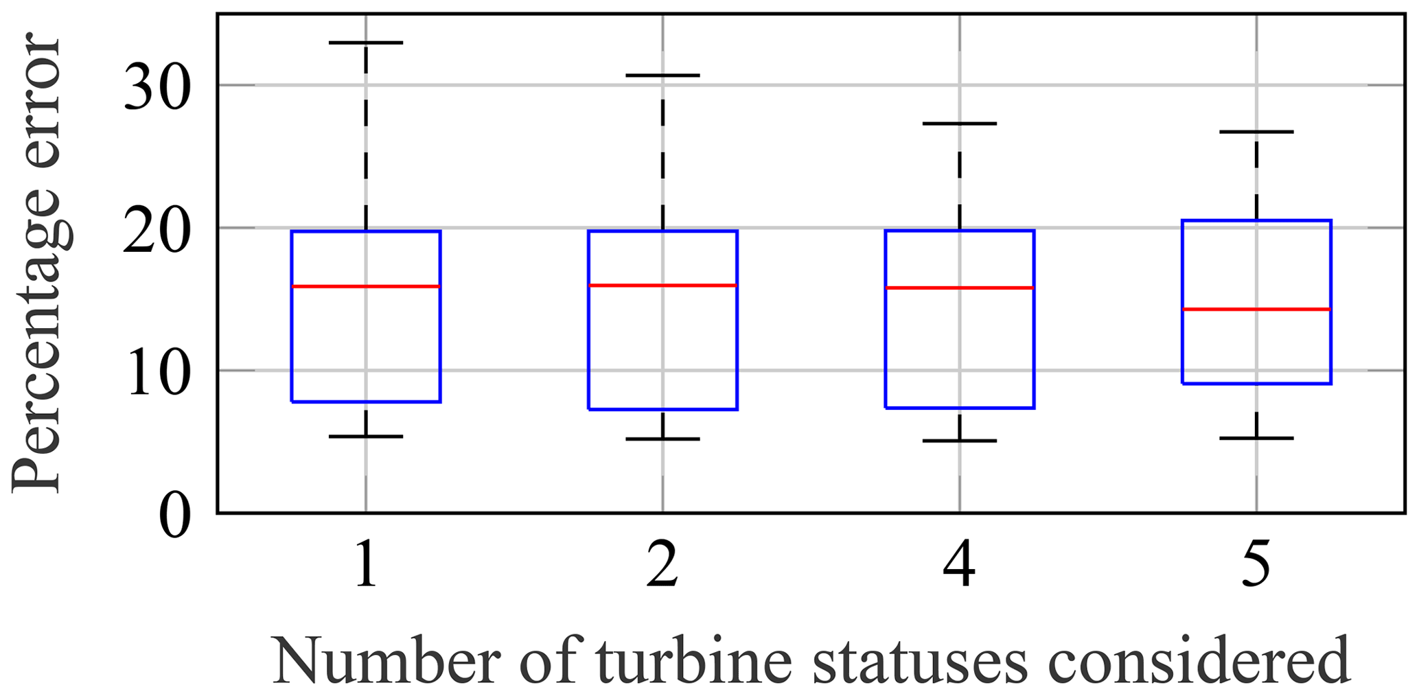
Figure 16 Percentage errors of predicted yearly damage values using simple extrapolation. Data separated according to turbine statuses: no separation (1), normal production operation and others (2), idling below cut-in and above cut-off (4), and service (5).

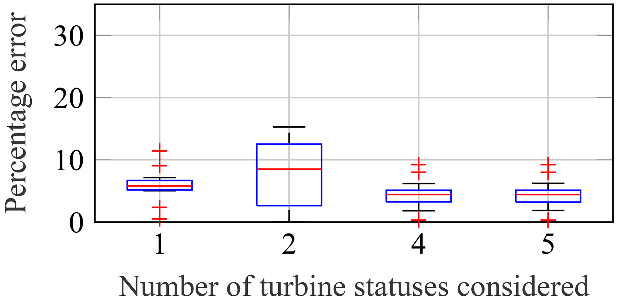
Figure 17 Percentage errors of predicted yearly damage values using a binning method (1D wind speed bins) compared to real yearly damage values. Data separated according to different turbine statuses (cf. Fig. 16).

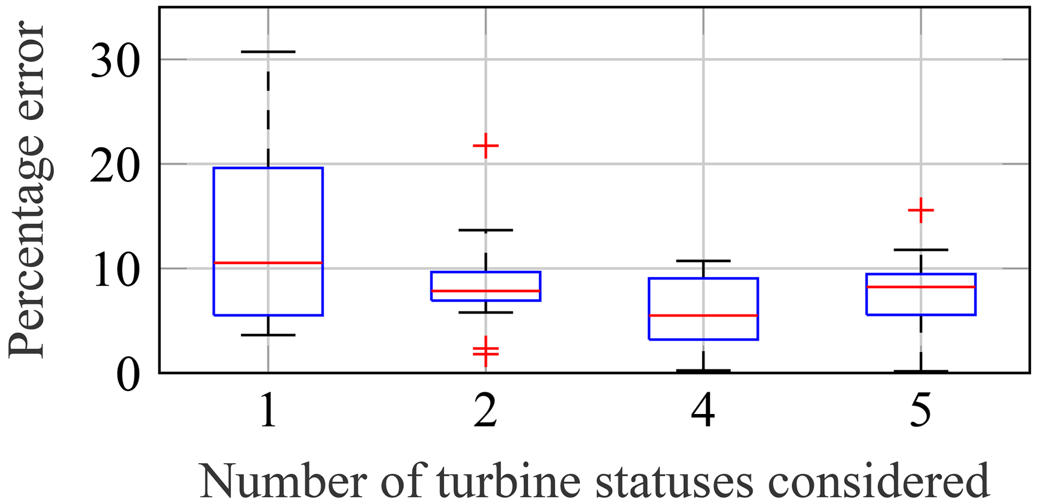
Figure 18 Percentage errors of predicted yearly damage values using an ANN compared to real yearly damage values. Data separated according to different turbine statuses (cf. Fig. 16).

To summarise, splitting up the data according to operational conditions can help to improve the extrapolation. However, it is not straightforward to determine the best separation, as it depends on the period considered and probably on the turbine as well. Moreover, if the measurement period is relatively short and/or many environmental conditions are taken into account, e.g. 3D binning, clustering according to operational conditions becomes more challenging. In this case, the amount of data for each turbine status might become insufficient.

Hence, as improvements are not always pronounced, for many applications it can be sufficient not to cluster the data according to operational conditions. This is especially the case either if the relation of operational to non-operational data is similar in the measurement and the extrapolation period or if the short-term damage values in operational and non-operational do not differ significantly. Since these two prerequisites are fulfilled for the present data, in the rest of this work, clustering according to operational conditions is not performed. In a real application, the two prerequisites should be checked. For example, the second prerequisite can easily be tested by analysing the difference between the mean short-term damage during operational and non-operational conditions in the measurement period.

4.2 Performance

In the following, the performance of the extrapolation approaches with respect to the accuracy of the prediction, the computing time, and the required data and knowledge is evaluated. For all methods, no clustering according to operational conditions is applied. For the binning approach, only wind speed bins with a bin size of 3 m s⁻¹ are used. Similarly, only wind speed correlations are taken into account for ANN and GPR. These choices are in accordance with the findings of Sect. 4.1.

In Fig. 19, the percentage errors of predicted yearly damage values of all approaches for all 13 years are shown. The limited accuracy of ANN and GPR in the present case is explained in more detail in the following.

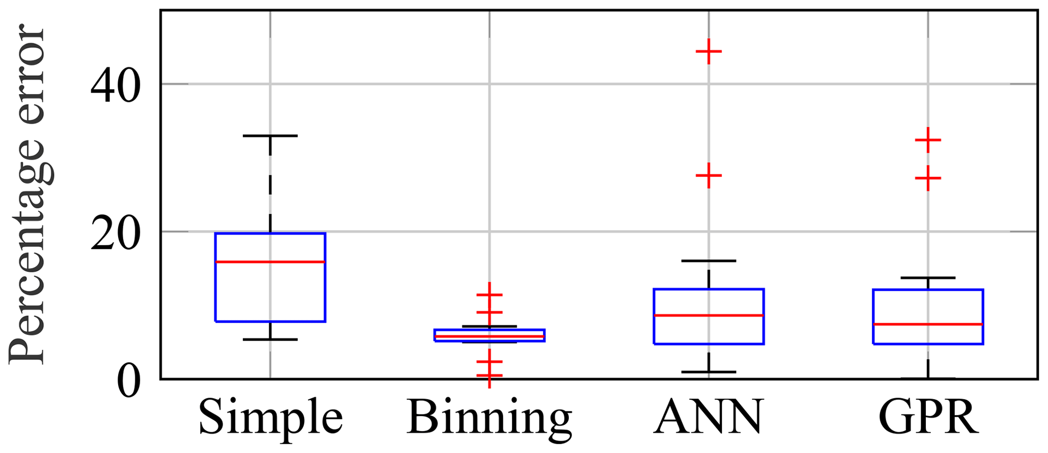
Figure 19 Percentage errors of predicted yearly damage values using all extrapolation methods compared to real yearly damage values. Predictions from a year to a second year for 13 different years.

It becomes apparent that the binning approach reduces the percentage error on average by about 60 % compared to the simple extrapolation (cf. red centre lines of the box plots). Moreover, the binning approach outperforms ANN and GPR. However, two facts about ANN and GPR should be mentioned. First, the initial weights used by ANN and the subsets used by GPR are chosen randomly. Hence, the performance of both is not deterministic but features some kind of model uncertainty that should not be confused with the uncertainty due to limited strain data (cf. Sects. 3.2.4 and 4.3). The existence of this model uncertainty – being relevant even when using precisely the same measurement/training data – becomes obvious when comparing the results of ANN and GPR (wind speed only) in Figs. 15, 18 and 19. All three figures show results for different randomly selected initial weights or subsets but the same measurement data. The box plots do not completely agree, although all settings, etc. are the same. Such a model uncertainty exists neither for the simple extrapolation nor for the binning approach. In order to assess the performance of ANN and GPR with some statistical evidence, several, e.g. 100, ANNs and GPR models are trained using the same training data but varying initial weights or subsets. The extrapolation results of the 100 trained models are averaged to rule out the model uncertainty. This yields mean percentage errors of the predicted yearly damage values of all 100 runs and 13 years of 10.3 % and 8.9 %, for each method, respectively. Hence, on average, both are outperformed by the binning approach, which yields a mean percentage error of all 13 years of 5.9 % (cf. red centre line of the box plot in Fig. 19). Second, it might be possible to improve the accuracy of the machine-learning approaches by exploiting their full potential, e.g. by using more hidden layers for ANN. However, a comprehensive analysis of the machine-learning approaches is beyond the scope of this work, as a user-friendly extrapolation approach is being sought. Moreover, d N Santos et al. (2021), who analysed ANN in more detail in the context of fleet-wide extrapolations, also found out that predictions – using 10 min SCADA data only – lead to percentage errors of up to 10 % in damage-equivalent loads. They showed that ANN is suitable for highly accurate predictions if more or better measurement data (e.g. 1 s SCADA data) are available but not for user-friendly predictions based on 10 min SCADA data, which are the focus of this work.

The second performance criterion evaluated in this work is the computing time. For deterministic predictions using wind speed as the only EOC, all methods are more or less suitable. For a prediction from a single year to another, the simple approach and the binning approach require less than 0.1 s on a standard desktop computer. ANN requires a few seconds, and GPR needs about 30 s. If ANN and GPR are run 100 times to rule out the model uncertainty, their computing times are significantly longer. For ANN, the computing time is still sufficiently short, i.e. only a few minutes. For GPR, 100 runs take nearly an hour. For probabilistic predictions, i.e. assessing the uncertainty due to limited strain data (cf. Sects. 3.2.4 and 4.3), thousands of predictions using different training data sets are required. Hence, the computing time becomes much more relevant. For example, if 1000 predictions are used for the uncertainty assessment, ANN and GPR require more than 30 min and more than 8 h, respectively, whereas the prediction based on bins is finished after about 10 s, and the simple prediction is finished within 1 to 2 s. At this point, it should be mentioned that the model uncertainty in ANN and GPR does not have to be treated separately for probabilistic predictions, i.e. 1000 and not 100×1000 runs. The reason for this is that some averaging of the model uncertainty is done implicitly when conducting predictions for 1000 different training data sets. Nonetheless, overall, the computing time of GPR is about 15 times higher compared to ANN. For ANN, it is more than 100 times higher compared to the binning approach and another 5 to 10 times higher compared to the simple approach. If additional EOCs are taken into account, the computing time of the binning approach increases quite quickly. For example, for three EOCs, the computing time of the binning approach increases by a factor of 5 compared to the case with a single EOC. For six EOCs, a probabilistic prediction already becomes unfeasible on a standard desktop computer for the binning approach. The reason for the increase is the extensive empty bin filling. For GPR, the increase is moderate. The computing time rises by factors of 1.5 to 2 and 4 to 5 for three and six EOCs, respectively. This increase is caused by the more complex training procedure needed for more inputs. For ANN, the computing time does not change significantly.

The last criterion, i.e. the user-friendliness and required data, is a more vague criterion. Clearly, the simple extrapolation does not require any additional data (e.g. SCADA data) and is straightforward to apply. The binning approach, especially if only wind speed bins are used, is also quite user-friendly and does not rely on detailed data. For the machine-learning approaches, first of all, much more expert knowledge is required to achieve adequate results. Moreover, the two previous criteria demonstrated that machine-learning approaches perform better with respect to accuracy and computing time if additional data (e.g. additional EOCs or 1 s SCADA data) are available.

To summarise, the simple extrapolation works relatively well. However, if 10 min SCADA data are available, the binning approach clearly outperforms the simple extrapolation with respect to accuracy, while computing time and user-friendliness are comparable. For expert users and high-quality data, ANN and GPR might be alternatives. For the current application, they are less accurate. Moreover, the machine-learning approaches, especially GPR, have significantly longer computing times. The long computing time of GPR makes probabilistic predictions nearly unfeasible on a standard desktop computer. This is why GPR is not considered in the rest of this work.

4.3 Uncertainty assessment

The box plots in the previous sections showed that the performance of the various extrapolation approaches depends on the period considered, as there is a significant scatter of the percentage error across the 13 different years. Since 13 different years are not enough for a well-founded assessment of the uncertainty of the prediction due to the limited available strain data, this uncertainty is approximated by applying bootstrapping, i.e. resampling with replacement. Therefore, for all three extrapolation approaches, bootstrapping is conducted using N_BT=1000 runs of resampling. This means that for each of the 1000 bootstrapping runs, 52 596 short-term damage values (D_j) are sampled with replacement from the measurement period (1 year in this section). Based on these short-term damage values, an entire extrapolation is conducted (see Sect. 3.2). For the binning approach, this means not only that mean damage values for all bins have to be calculated 1000 times but also that empty bins have to be filled up for each bootstrap run as well. For ANN, a new functional relationship f(x) has to be determined 1000 times using the “new” training data. As stated before, the effect of random initial weights is no longer relevant for ANN, since some averaging takes place implicitly during the 1000 bootstrap runs. For all approaches, the same settings as before are used, e.g. only wind speed bins. The bootstrapping yields N_BT values for the extrapolated yearly damage D_pred. These values are compared to the real damage values for the second year to calculate an empirical distribution for the percentage error. In this case, signed percentage errors are used – i.e. no absolute values of errors – to analyse the bias of the extrapolation as well. Example resulting empirical distributions are shown in Fig. 20 for an extrapolation from a single year (1 October 2015 to 30 September 2016) to another year (1 October 2016 to 30 September 2017). The results demonstrate that there is some uncertainty in the extrapolation, which should not be neglected. Moreover, all approaches lead to slightly biased results. This is not surprising, since the correlation between the environmental conditions and fatigue damage cannot cover all effects. Nonetheless, this bias is not critical, as it is not systematic. For some measurement periods, the extrapolation is conservative, but for others it is not (cf. Figs. 20 and 21). Such (random) changes in conservatism are typical of approaches using correlations. Depending on the “severity” of all other (not considered) EOCs during the measurement and extrapolation period, the results will be conservative or not. If it is necessary to be conservative in all cases, an option could be, for example, to use a high percentile of the resulting distribution (cf. Fig. 20 and 21).

Figure 20 Empirical distribution for the (signed) percentage error of predicted yearly damage using different extrapolation methods. Prediction from a single year (1 October 2015 to 30 September 2016) to another year (1 October 2016 to 30 September 2017). PDF: probability density function.

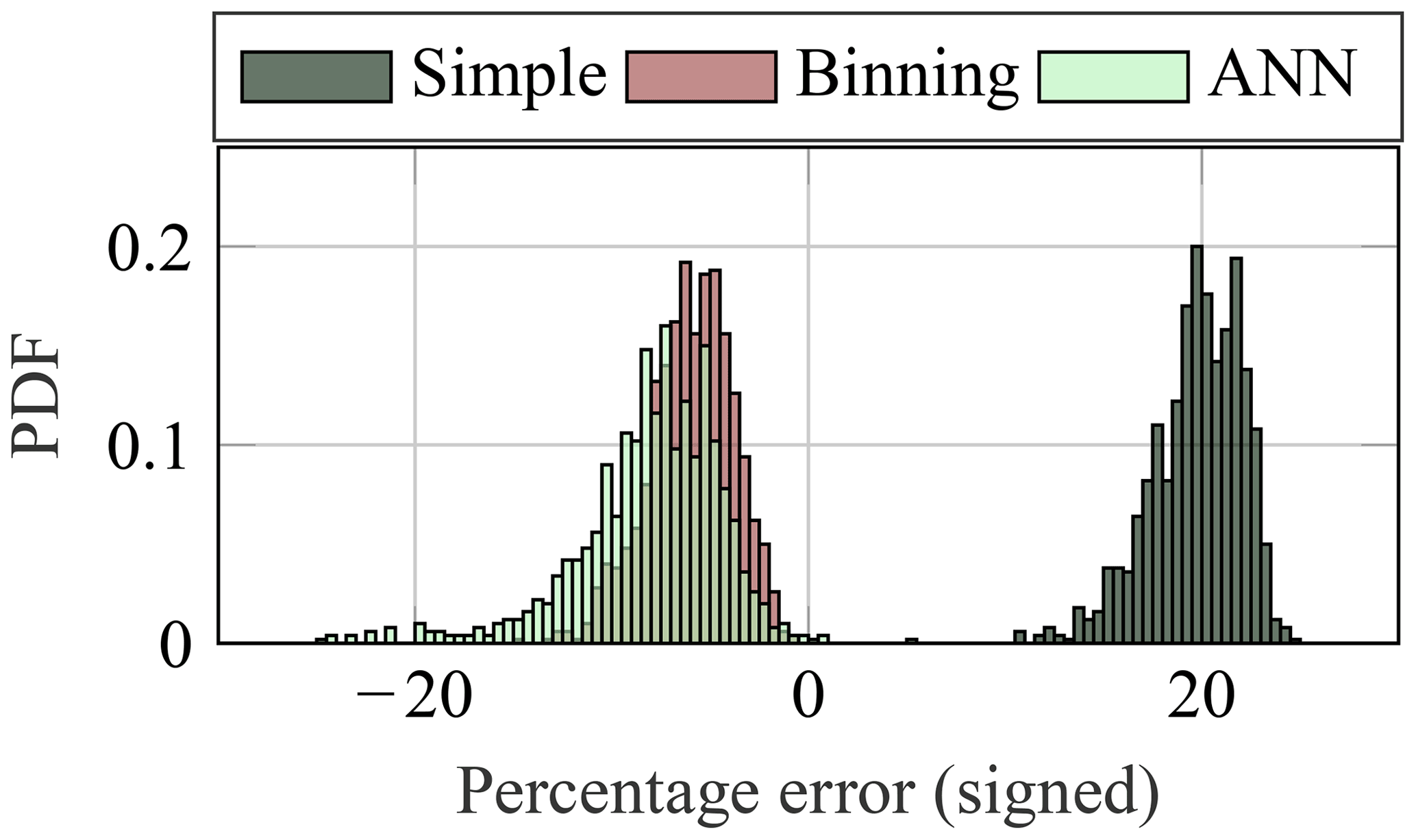
Figure 21 Empirical distribution for the (signed) percentage error of predicted yearly damage using different extrapolation methods. Prediction from a single year (1 August 2016 to 31 July 2017) to another year (1 October 2015 to 31 July 2016 and 1 August to 30 September 2017). PDF: probability density function.

Overall, even the highest errors are below ±20 % for the binning approach. Finally, it should be noted that the variance of the distributions for the binning approach (cf. Figs. 20 and 21) is smaller compared to the other approaches. Hence, the binning approach features the lowest uncertainty. The reason for the higher uncertainty for ANN is the randomness of the initial weights that is covered implicitly by the bootstrapping. Compared to the simple extrapolation, the binning approach has a slightly reduced uncertainty, as the scattering of the short-term damage values D_j within each bin is smaller compared to the scattering if no bins are employed.

4.4 Minimum measurement length

In theory, the three extrapolation methods can be used to extrapolate from any period to another. However, if the measurement length is too short, the extrapolation will be biased (Hübler et al., 2018). A simple example in this context is that an extrapolation based on data from a few summer months with benign environmental conditions will lead to an underestimation of the fatigue damage for winter months. Therefore, in the following, the convergence of the percentage error of the predicted yearly damage with increasing measurement length is analysed to determine a minimum measurement length. This analysis is conducted for all three extrapolation approaches using the same settings as before.

Measurement lengths of 2 to 12 months are used to predict the fatigue damage expected to occur in a second year. This means that, for example, 1 October to 30 November 2015, 1 October to 31 December 2015 and so on are extrapolated to the second year, i.e. 1 October 2016 to 30 September 2017. Again, to enable a statistical interpretation of the results, these predictions using different measurement lengths are repeated using the 13 different years that have been used before, e.g. 1 November to 31 December 2015 is extrapolated to October 2015 and 1 November 2016 to 30 September 2017 (cf. Fig. 12). This yields 13 different values for 11 different measurement lengths. The results for all three approaches are shown in Figs. 22 to 24.

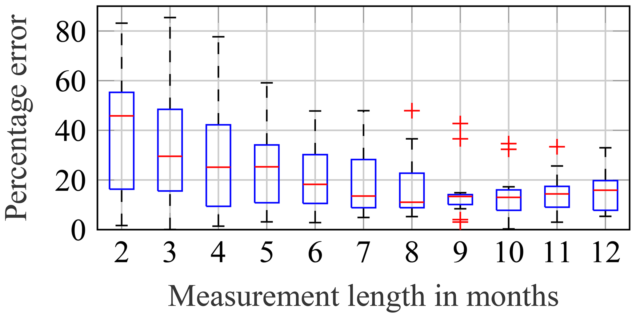
Figure 22 Convergence of the percentage error of predicted yearly damage values using simple extrapolation for increasing measurement lengths. Box plot shows data from 13 different measurement periods.

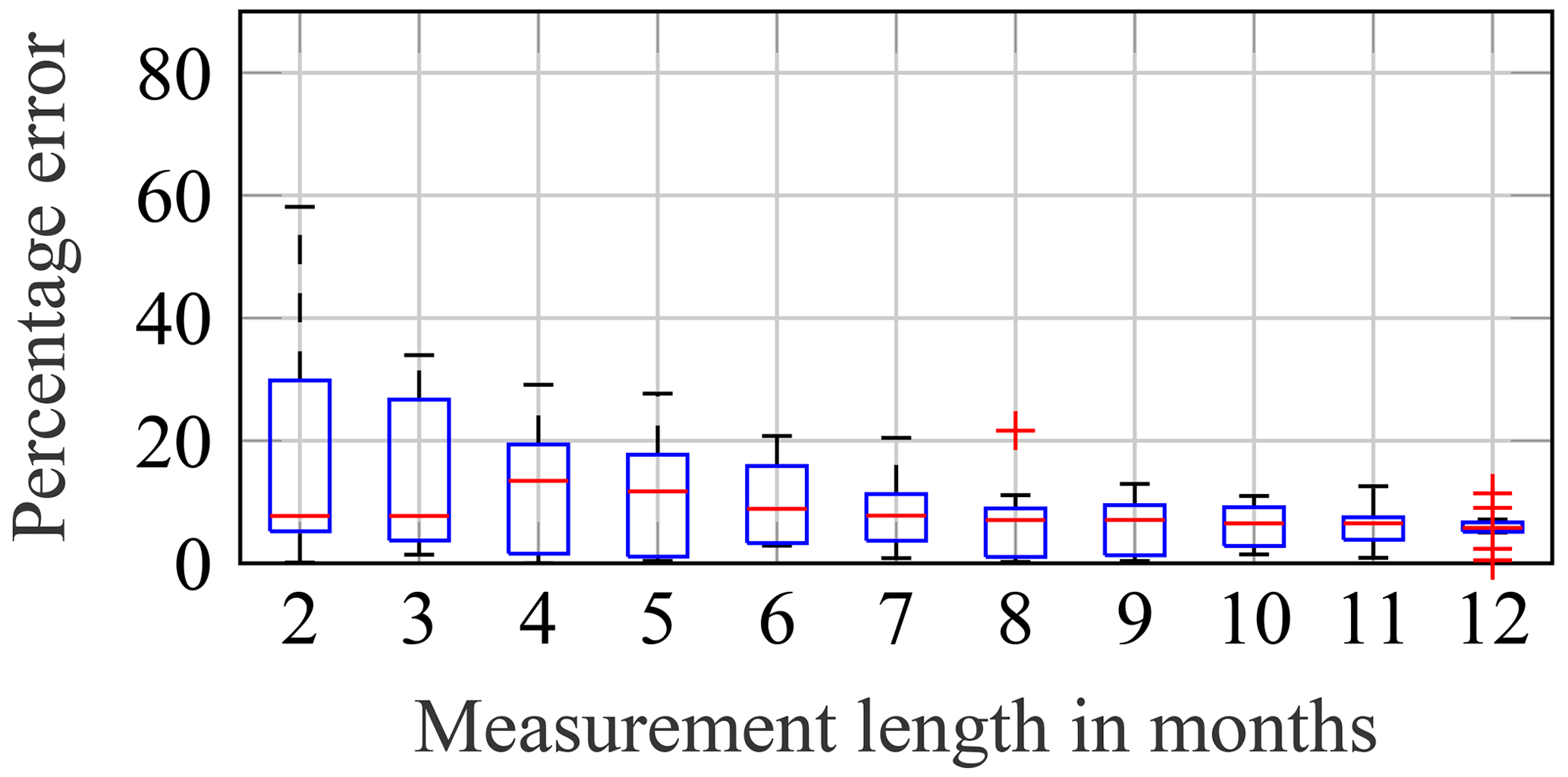
Figure 23 Convergence of the percentage error of predicted yearly damage values using the binning approach for increasing measurement lengths. Box plot shows data from 13 different measurement periods.

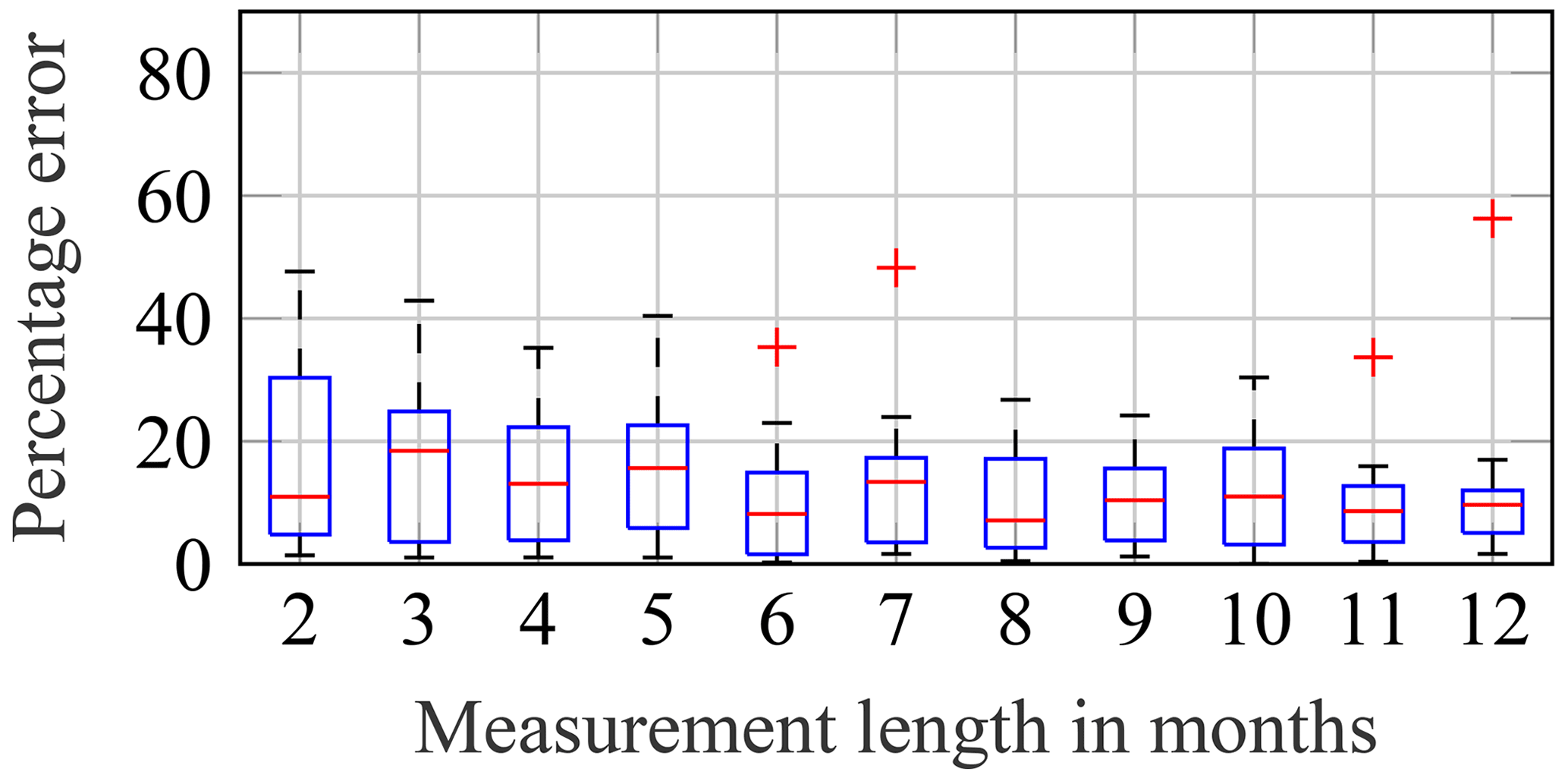
Figure 24 Convergence of the percentage error of predicted yearly damage values using the ANN for increasing measurement lengths. Box plot shows data from 13 different measurement periods.

For the simple approach, no complete convergence is achieved even for measurement lengths of 12 months. There is a small increase in the percentage error for measurement lengths of more than 9 months. This is probably a statistical artefact due to the limited number of different measurement periods. Nonetheless, for measurement lengths greater or equal to 9 months, relatively low percentage errors are achieved. This is not only in accordance with results from Hübler et al. (2018), who recommended a minimum measurement length of 9 months, but also logical. In order to cover seasonal effects, nearly a complete year has to be measured.

For the binning approach, convergence is achieved for measurement lengths of approximately 8 to 9 months. After this period, all bins – especially those for high wind speeds are critical – are filled with enough data for an accurate extrapolation. However, for the binning approach, this time can be reduced if the measurement period starts during the winter. Figure 25 shows the same convergence plot but only for starting dates of the measurement period between 1 October and 1 February. For these starting dates, the relevant bins are filled with enough data within a few months. After 2 or 3 months, sufficient data might already be available; after a few months, additional data do not improve the prediction. The slight increase in percentage errors for measurement lengths of 10 months and more – visible in Fig. 25 – is probably only due to the limited number of different measurement periods – in this case, five. To sum up, if binning approaches are to be used, it might be expedient to start measurement campaigns in the autumn.

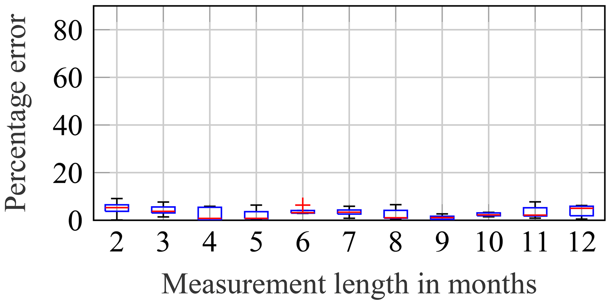
Figure 25 Convergence of the percentage error of predicted yearly damage values using the binning approach for increasing measurement lengths. Box plot shows data from five different measurement periods starting in the winter.

For ANN, fairly accurate results can be achieved using data from a few months. Here, the advantage of determining a functional relationship becomes obvious if data are scarce. Starting the measurement campaign in winter can further reduce the required measurement length (not shown). Nonetheless, it should be noted that even for a measurement length of only 2 months, ANN and the binning approach perform similarly well.

4.5 Long-term extrapolations

So far, all extrapolations of fatigue damage have been conducted for 2 consecutive years, i.e. short-term extrapolations. This has the advantage that long-term changes not only in the environmental conditions but also in the turbine can virtually be ruled out. However, for real damage assessments used for lifetime extensions, an extrapolation over several years might be necessary. For example, if strain gauges failed after 5 years of operation and an lifetime extension is planned after 15 years, extrapolations over 10 years, i.e. long-term extrapolations, are required. Such long-term extrapolations might be more challenging, as the “learned” correlation between environmental conditions and fatigue damage might have changed. If it has changed, which might even happen within the first year after the measurement campaign ended, extrapolations based on all three methods are impossible. It is important to be aware of this fact. Otherwise such effects might lead to an underestimation of the fatigue loads.

In the following, a single year of measurement data is extrapolated to a second year which occurred several years earlier or later. For this purpose, data from the 3 years of 1 January to 31 December 2011 and 1 October 2015 to 30 September 2017 are used. Similar to before, the starting dates of the 2 years are shifted month by month in order to realise a higher number of different years. This means that the year of 1 January to 31 December 2011 is extrapolated forwards to 1 October 2015 to 30 September 2016, 1 November 2015 to 31 October 2016 and so on. In addition, 1 October 2015 to 30 September 2016, 1 November 2015 to 31 October 2016 and so on are extrapolated backwards to 1 January to 31 December 2011, i.e. vice versa. This procedure yields 26 different years. A visualisation of this shifting procedure is shown in Fig. 26.

Figure 26 Visualisation of the 26 different periods for statistical evaluations in the context of long-term extrapolations.

The results of the long-term extrapolation for the three extrapolation approaches, using the same settings as before, are shown in Fig. 27 and compared to the previously determined results of the short-term extrapolations.

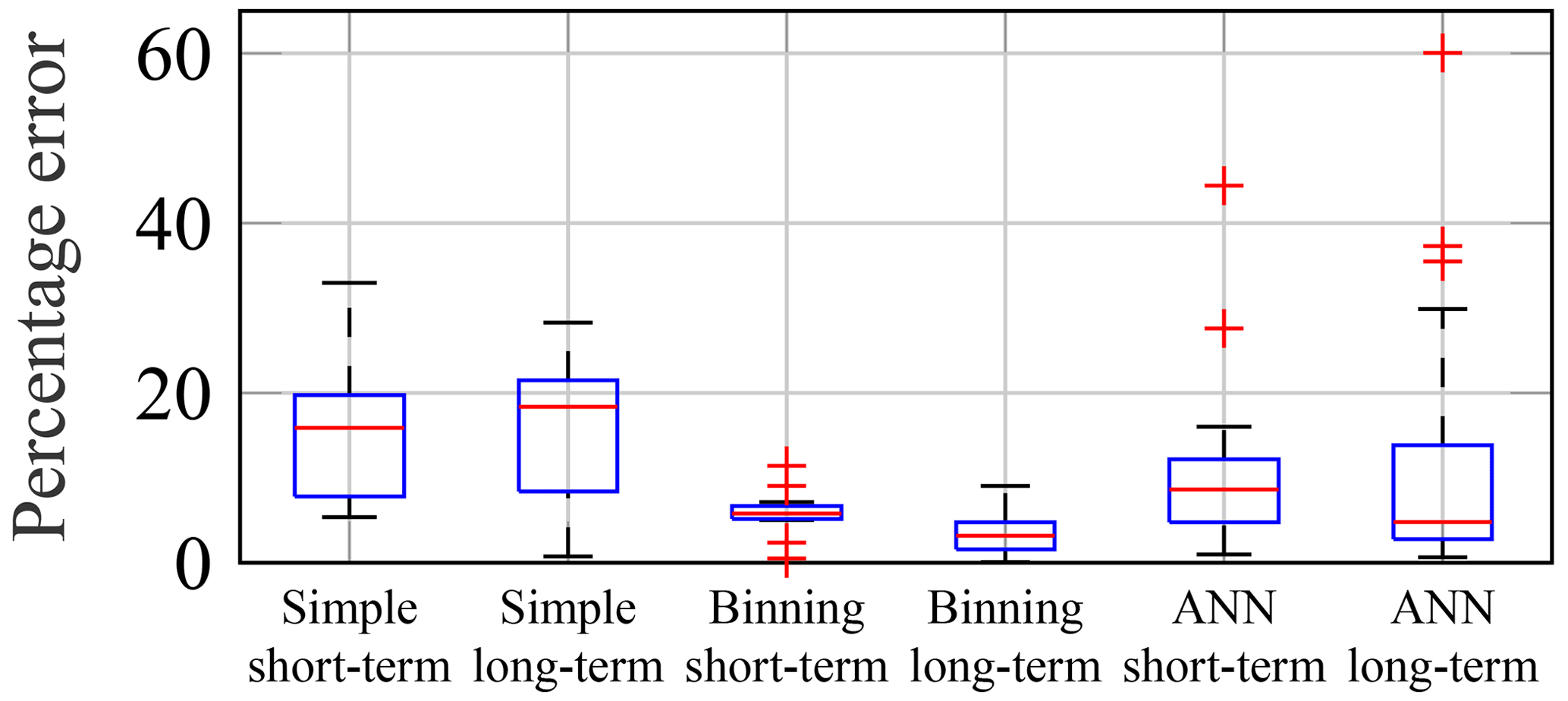
Figure 27 Percentage errors of predicted yearly damage values using all extrapolation methods compared to real damage values. Data concern both short-term (13 different consecutive years) and long-term predictions (1 year extrapolated to a non-consecutive second year for 26 different years).

For all three extrapolation approaches, the resulting percentage errors are in a similar range for both short-term and long-term extrapolations. For the binning approach, the approximation even improves slightly for long-term extrapolations. However, it can be assumed that this improvement is only due to some random effects in the varying environmental conditions across the different years. Nonetheless, for this data set, it can be concluded that long-term changes in the structural behaviour seem to be less pronounced compared to variations in environmental conditions. Therefore, depending on how severe structural changes are, i.e. whether the learned correlation is still valid, long-term extrapolations are possible, especially if the binning approach is applied. Certainly, it must be asked where the boundaries of these long-term extrapolations lie. Is it still possible to use them if the structure has changed significantly (e.g. rotor blades have been exchanged)? This question cannot be answered conclusively by this work, as much more data would be needed and since the answer will always be case-specific to some extent. Nonetheless, although the exact changes to the AV-07 turbine may not be mentioned here for reasons of confidentiality, it should be said that the AV-07 turbine has been significantly modified during the period considered. Despite this significant modification, the learned correlation seems to be still valid. Hence, long-term extrapolations are probably possible for more situations than expected, sometimes even if moderate to severe modifications to the turbine have been made. In a real industry application, it would be necessary to test the validity of the correlations every few years. For this purpose, for example, a small measurement campaign with only strain gauges at a single location for a few weeks could be conducted.

4.6 Extrapolation to the future

In all previous sections, it has been shown that the use of EOC data, i.e. SCADA data, is beneficial compared to a simple extrapolation based on pure strain data. However, it was always assumed that EOC data are available for the predicted period. This is a valid assumption for nearly all predicted periods in the past, since SCADA systems feature a high availability and data quality. However, for extrapolations into the future, this is no longer valid. Extrapolations into the future are especially relevant for lifetime extensions. Hence, in this section, the last question of Sect. 4, i.e. “Do the approaches still yield reasonable results if extrapolations into the future are conducted, for which no EOC data are available?”, is to be answered. For this purpose, the binning probabilities ($P{r}_{\text{pred},i_{\mathrm{1}},\mathrm{\dots },i_d}$) in Eq. (8) are no longer determined using EOC data from the predicted (future) period. Instead, past long-term EOC data are used. Long-term EOC data should be available for any lifetime extension, as the wind turbine has already been operating for 15 to 20 years. Moreover, it can be assumed that EOCs in the future period can be better predicted using long-term EOC data compared to using EOC data from the limited measurement period, i.e. the period for which strain data are available. The advantage of long-term EOC data is that random variations are more completely included. Using only EOC data from the measurement period could yield biased results if, for example, the measurement period features relatively harsh conditions compared to the long term. This is why, in this work, long-term probabilities for all wind speed bins ($P{r}_{\text{long-term},i_{\mathrm{1}},\mathrm{\dots },i_d}$) are determined using EOC data from 10 years (2011 to 2020). Using the long-term probabilities, an extrapolation to future periods should be possible, even if no EOC data are available for the predicted period:

$$\begin{array}{}\text{(15)}& D_{\text{future}}\approx N_{\text{n}}\sum _{i_{\mathrm{1}}=\mathrm{1}}^{M_{\mathrm{1}}}\mathrm{\dots }\sum _{i_d=\mathrm{1}}^{M_d}\left(P{r}_{\text{long-term},i_{\mathrm{1}},\mathrm{\dots },i_d}{\stackrel{\mathrm{‾}}{D}}_{i_{\mathrm{1}},\mathrm{\dots },i_d}\right).\end{array}$$

For approaches using functional relationships, the adaptation for future periods is similar. Here, Eq. (11) remains nearly unchanged. The only difference is x_k. For predictions into the past, x_k is the EOCs of the predicted period, i.e. ${\mathbf{x}}_k\in \left\{{\mathbf{x}}_{\mathrm{1}},\mathrm{\dots },{\mathbf{x}}_{N_n}\right\}$. For predictions into the future, N_n random realisations (with replacement) of the EOCs of the long-term measurement period are generated, i.e.

$$\begin{array}{}\text{(16)}& D_{\text{future}}\approx \sum _{k=\mathrm{1}}^{N_n}f\left({\mathbf{x}}_k\right){\mathbf{x}}_k\in \left\{{\mathbf{x}}_{\mathrm{1}},\mathrm{\dots },{\mathbf{x}}_{N_{\text{long-term}}}\right\},\end{array}$$

where N_long-term is the number of short-term, e.g. 10 min, intervals in the long-term measurement period.

For the simple extrapolation, there is no difference between extrapolations to periods in the past (with available EOC data) and the future (without EOC data), since the simple extrapolation is based on strain data from the measurement period only.

Results of all three approaches are shown in Fig. 28. In this figure, percentage errors of predicted yearly damage for future periods are compared to previous results for which EOC data are available (short-term predictions of past periods).

Figure 28 Percentage errors of predicted yearly damage values using all extrapolation methods compared to real yearly damage values. Results of predictions into the future using long-term EOC data are compared to previous results for which EOC data are available (short-term predictions of past periods); 13 different years are used in both cases.

By definition, for the simple extrapolation, an extrapolation into the future is equally accurate compared to an extrapolation to a period for which EOC data are available. For all other approaches, the results demonstrate that the quality of the prediction decreases slightly for extrapolations into the future. Nonetheless, predictions are still reasonable and yield lower percentage errors compared to the simple extrapolation. Just like before, the binning approach also leads to the smallest percentage errors for extrapolations into the future.

In summary, extrapolations to future periods, for which no EOC data are available, are still possible with a relatively high accuracy provided that past long-term EOC data are used instead. Again, the binning approach is most suitable. Certainly, it must be kept in mind that the accuracy will decrease if long-term changes in the EOCs, e.g. due to climate change, become relevant. Hence, an accurate extrapolation of a few years into the future is possible, but an extrapolation 20 years into the future might be unreasonable.

5 Conclusion, benefits and limitations

To enable well-founded lifetime extensions for OWTs, the remaining useful lifetime has to be determined. Although several simulation-based and strain-measurement-based approaches for determining the remaining useful lifetime already exist, especially for strain measurement concepts, additional research is required. This work addresses the research gap regarding extrapolations of strain-measurement-based fatigue damage calculations to other time periods.

Regarding the extrapolation in time, several approaches making use of the correlation of EOCs (10 min mean values) and short-term fatigue damage values are enhanced, assessed and validated using real offshore measurement data. The approaches are a simple extrapolation, a binning approach and two machine-learning approaches. A summary of the most important results is as follows.

1. User-friendly binning approaches yield accurate results.

2. More complex machine-learning approaches do not yield better results for the given data type, i.e. 10 min EOC data.

3. It is sufficient to consider wind speed correlations only. Other environmental conditions do not need to be taken into account for locations at the tower.

4. Consideration of different turbine statuses can improve the accuracy of the prediction. However, as it is not straightforward, careful consideration should be given to the question of whether it is beneficial.

5. The uncertainty of the prediction is moderate, and no systematic bias occurs.

6. It is sufficient to measure strains for only a few months, if these months are winter months.

7. Long-term extrapolations over several years might be possible, even if the OWT is moderately to heavily modified in this time period if the learned correlation between EOCs and fatigue damage is still valid, which has to be checked.

8. For extrapolations into the future, the accuracy of the prediction decreases, since EOCs have to be approximated using long-term EOC data. Still, reasonable predictions are possible.

Therefore, the results of this work demonstrate that user-friendly binning approaches are a suitable alternative or addition to simulation-based lifetime extensions, even if only limited strain data are available. However, some limitations of this work should be discussed. First, spatial extrapolations, i.e. extrapolations to other locations on the same turbine and/or to other turbines in the same wind farm, are not addressed. For spatial extrapolations, the reader is referred to current research, e.g. Noppe et al. (2020) or Ziegler et al. (2019). Second, to determine correlations, only data of various environmental conditions and the turbine status are used in this work. Classical continuous operational conditions, like power output, are not taken into account. There are well-founded reasons why wind speed data in combination with the turbine status are used instead of power output data. For example, power output data have no informative value for all turbine statuses where the turbine is not operating. Still, an additional use of continuous operational conditions might be expedient. Third, only 10 min data are used. This is reasonable, since 10 min SCADA data are nearly always available. Nonetheless, d N Santos et al. (2021) already showed that additional data, e.g. 1 s SCADA data, are valuable for machine-learning approaches. Fourth, all present analyses are only conducted for one turbine and one location. Since other studies using different turbines – e.g. Hübler et al. (2018) – yield comparable results, we do not expect significant changes for similar turbines and/or other locations on the substructure and/or tower. It could just be the case that the influence of wave loads increases for locations further down the turbine. For completely different turbines – e.g. floating OWTs – results might no longer be valid. Moreover, for locations on the blades, the assumption of linear damage is at least questionable. Hence, to determine the remaining lifetime of blades accurately, the approaches might need to be adapted slightly. Finally, the analysed turbine is located in the North Sea. There, only small to moderate long-term changes in the environmental conditions occurred during the measurement period. For other locations and/or accelerating climate change, significant long-term changes in environmental conditions might occur. This might reduce the accuracy of the binning approach, even though the bin probabilities should cover most of these changes.

6 Outlook

Some of the previously mentioned limitations of this work immediately lead to future work.

First, the results of this work should be assessed for other turbine types, for example, in other regions of the world or onshore. This would increase the general validity of the results. Certainly, here, the availability of open-access strain measurement data is a limiting factor.

Second, an analysis of extrapolation approaches for turbine blades would be valuable. The presented binning approach is quite user-friendly and based on limited data. Hence, it could be interesting for industry applications. If such a “simple” approach were available for blades and other components as well, this could be a useful extension. However, before applying the binning approach to rotor blades, two simplifications of the short-term damage calculations should be investigated in more detail. The relevance of sequence effects of stress cycles has to be investigated. Moreover, the effect of long-term fatigue cycles lasting more than an hour should be analysed. For such cycles, Marsh et al. (2016) and Sadeghi et al. (2022) showed their relevance even for steel components of wind turbines. Two approaches to reduce the error due to long-term fatigue cycles could be to increase the length of the short-term periods to several hours or to derive a correction factor (i.e. a damage ratio of damage values with and without consideration of long-term fatigue cycles) similar to Marsh et al. (2016) and Sadeghi et al. (2022).

Third, the value of additional data, e.g. data of continuous operational conditions like power output or pitch angle or 1 s SCADA data, should be analysed. For machine-learning approaches, additional data are valuable. However, it is not known whether it also improves the accuracy of binning approaches, since these are normally based on aggregated EOC data.

Fourth, a thorough comparison with the probabilistic approach of Mai et al. (2019) would be interesting, especially when focussing on the amount of required measurement data.

Finally, a combination of temporal and spatial extrapolation methods would be an interesting addition. In this context, spatial extrapolations cover predictions for other positions on the same turbine and also for other turbines in the same wind farm.

Appendix A: Use of SCADA data

In this work, environmental conditions are taken from the FINO1 met mast. Only if no data are available from FINO1, are the wind conditions included in the SCADA data from the AV-07 turbine taken into account. The reason for using FINO1 data is that they are of higher quality. Still, in industry applications, met mast data are normally not available. Hence, the proposed methods have to yield accurate results even if only SCADA data are used. In theory, this should be the case, since EOC data are only used for the correlation, e.g. binning. The practical applicability is demonstrated in Fig. A1. It shows – exemplarily for the 1D binning approach – a comparison of extrapolation results based on met mast plus SCADA data (cf. Fig. 14) and pure SCADA data.

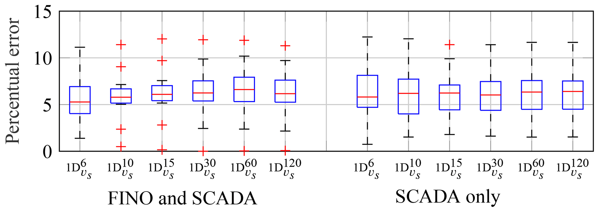
Figure A1 Percentage errors of predicted damage values using a binning method compared to real damage values. Comparison of predictions using met mast plus SCADA data and SCADA data only. Results only for 1D bins, i.e. wind speed (v_s) bins, but various bin sizes (n). Notations as before: ${\text{1D}}_x^n$.