Atmospheric rotating rig testing of a swept blade tip and comparison with multi-fidelity aeroelastic simulations

One promising design solution for increasing the energy production of modern horizontal axis wind turbines is the installation of curved tip extensions. However, since the aeroelastic response of such geometrical add-ons has not been characterized yet, there are currently uncertainties in the application of traditional aerodynamic numerical models. The objective of the present work is twofold. On the one hand, it represents the first effort in the experimental characterization of curved tip extensions in atmospheric flow. On the other hand, it includes a comprehensive validation exercise, accounting for different numerical models for aerodynamic load prediction. The experiments consist of controlled field tests at the outdoor rotating rig at the Risø campus of the Technical University of Denmark (DTU), and consider a swept tip shape. This geometry is the result of an optimized design, focusing on locally maximizing power performance within load constraints compared to an optimal straight tip. The tip model is instrumented with spanwise bands of pressure sensors and is tested in atmospheric inflow conditions. A range of fidelities of aerodynamic models are then used to aeroelastically simulate the test cases and to compare with the measurement data. These aerodynamic codes include a blade element momentum (BEM) method, a vortex-based method coupling a near-wake model with a far-wake model (NW), a lifting-line hybrid wake model (LL), and fully resolved Navier–Stokes computational fluid dynamics (CFD) simulations. Results show that the measured mean normal loading can be captured well with the vortex-based codes and the CFD solver. The observed trends in mean loading are in good agreement with previous wind tunnel tests of a scaled and stiff model of the tip extension. The CFD solution shows a highly three-dimensional flow at the very outboard part of the curved tip that leads to large changes of the angle of the resultant force with respect to the chord. Turbulent simulations using the BEM code and the vortex codes resulted in a good match with the measured standard deviation of the normal force, with some deviations of the BEM results due to the missing root vortex effect.

1 Introduction

The trend of reducing the levelized cost of energy (LCOE) of horizontal axis wind turbines through increasing rotor size has long been established. To achieve this, the challenges of scaling must be overcome through innovative turbine design and control strategies (Veers et al., 2019). One promising blade design concept is advanced aeroelastically optimized blade tip extensions, which could drive rotor upscaling in a modular and cost-effective way.

Existing bibliography relevant to wind turbine applications typically focuses on winglets and aerodynamic tip shapes, with limited testing of generalized curved shapes in controlled or atmospheric conditions (Johansen and Sørensen, 2006; Gaunaa and Jeppe, 2007; Gertz et al., 2012; Hansen and Mühle, 2018; Sessarego et al., 2020).

Previous related work by the authors focused on the aeroelastic optimization of curved tip extensions (Barlas et al., 2021a) and wind tunnel testing (Barlas et al., 2021b). In the present work, the aeroelastic response of a swept tip extension is investigated for application to horizontal axis wind turbines. Controlled field testing is performed using the outdoor rotating test rig (RTR) at the Technical University of Denmark (DTU). The swept tip shape in focus is the result of a design optimization focusing on locally maximizing power performance within load constraints compared to an optimal straight tip for testing in the RTR. The tip model is instrumented with spanwise bands of pressure sensors and is tested in atmospheric inflow conditions. A range of fidelities of aerodynamic models are used to aeroelastically simulate the test cases and results are compared with the measurement data, namely a blade element momentum (BEM) model, a vortex-based method coupling a near-wake model with a far-wake model (NW), a lifting-line hybrid wake model (LL), and fully resolved Navier–Stokes simulations (CFD).

2 Tip model design

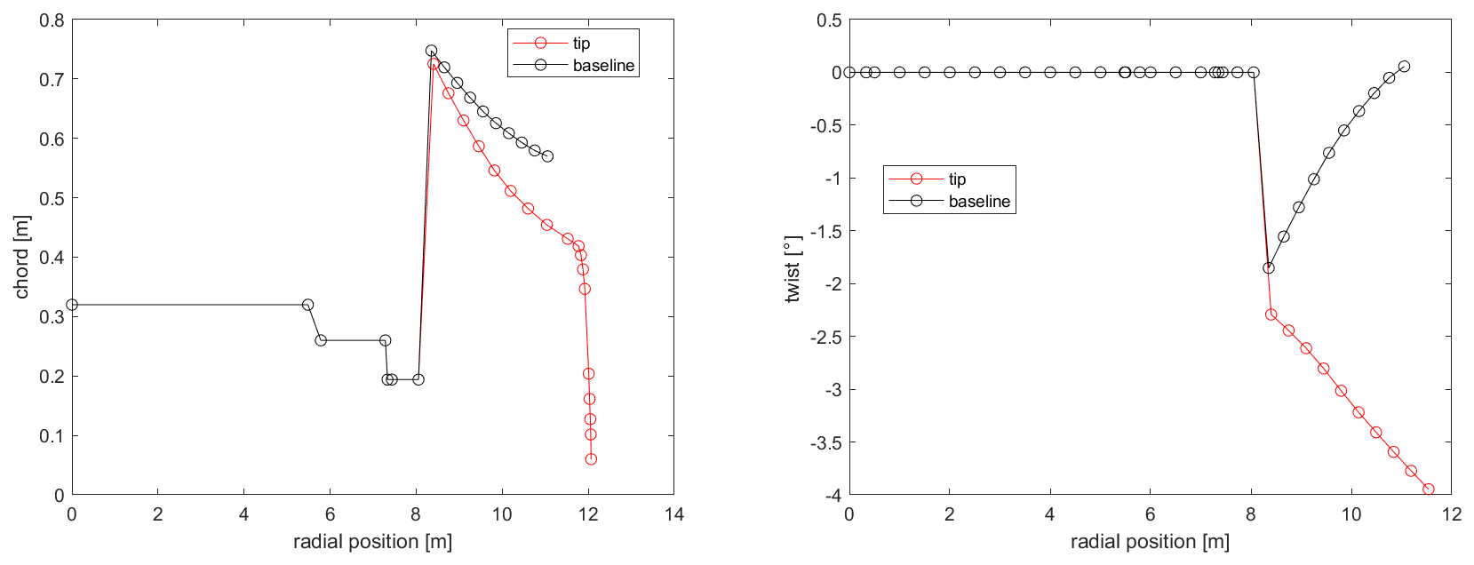
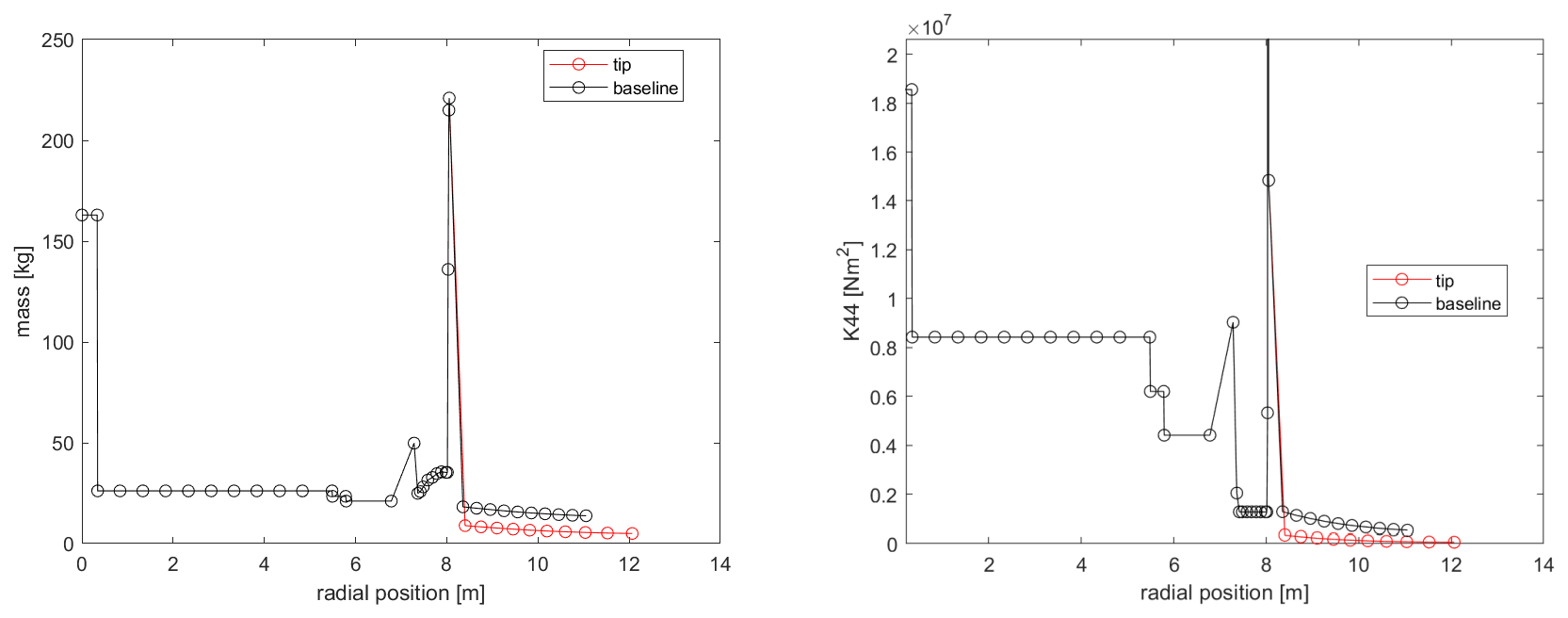
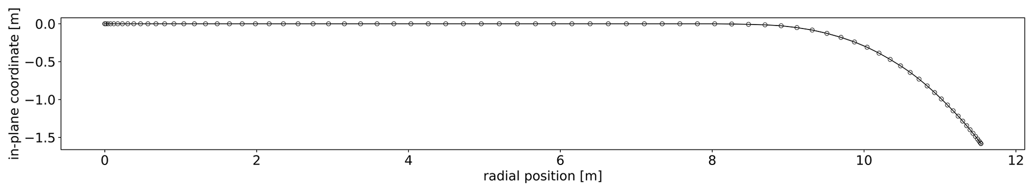
The tip shape presented in this work is an aeroelastically optimized tip which is mounted on DTU's rotating test rig (RTR) (Madsen et al., 2015; Ai et al., 2019), whereas a scaled stiff version of it has been tested in the wind tunnel (Barlas et al., 2021b). The design-optimization method used is described in Barlas et al. (2021a) for a tip extension on a full-scale wind turbine. The method of optimizing the tip for the RTR is essentially the same, while the baseline geometry and load envelope is defined by a reference straight tip designed for optimal BEM performance on a three-bladed rotor (Table 1). Additionally, the structural sectional layup of the tip is parameterized using the BECAS software (Blasques et al., 2015). The reference tip is designed using the FFA-W3-211 airfoil with fully turbulent wind tunnel polars (Bertagnolio et al., 2001) for a Reynolds number of 1.78×10⁶, with a predefined length of 3 m (practical design constraint for testing on the outdoor rotating rig) mounted on the 8 m cylindrical boom of the RTR. The cylindrical sections of the boom are modeled with a drag coefficient of 0.8 and zero lift. The chord and twist distributions of the straight tip were determined from the BEM performance for an optimal power coefficient in operation at 30 rpm with 6 m s⁻¹ inflow wind speed (tip speed ratio of 4.5–6 along the tip). The resulting aeroelastically optimized tip maximizing power performance within load constraints, utilizing sweep (Fig. 1), achieved a 19.58 % increase in power with the baseline ultimate flapwise bending moment at the boom root and tip connection, when evaluated at an extreme turbulence case (class III-C) at 6 m s⁻¹ in the aeroelastic code HAWC2 (Larsen and Hansen, 2007) using the near wake (NW) model (Madsen and Rasmussen, 2004; Pirrung et al., 2016, 2017a, b; Li et al., 2022). Since the RTR is a powered setup, the local power changes cannot be translated to any meaningful full-scale turbine application, but are simply used in the design optimization herein. The Pareto front of the design-optimization solutions is shown in Fig. 2. The design features a highly swept (in-plane offset) centerline (Fig. 3), slender chord distribution, and negative twist (to feather) distribution (Fig. 4) compared to the reference straight tip, whereas the airfoil sections are aligned perpendicular to the centerline. The very last tapering of the tip chord is only relevant for the fully resolved Navier–Stokes modeling, whereas the optimized chord distribution from the NW model stops at a finite chord of 0.41 m at the 12 m span location. The optimized mass and flapwise stiffness distribution as well as the structural layup are shown in Figs. 5 and 6.

Table 1 Design variables range and optimized values.

Figure 1 Three-dimensional geometry of the tip indicating the measurement sections.

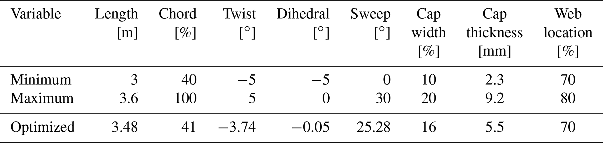
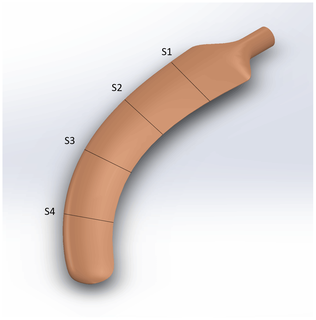
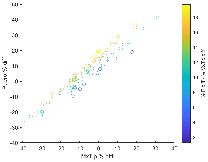
Figure 2 Pareto front of the optimization objectives (horizontal axis: change in flapwise bending moment at tip connection compared to baseline, vertical axis: change in aerodynamic power compared to baseline, color bar: summed difference in power and flapwise moment).

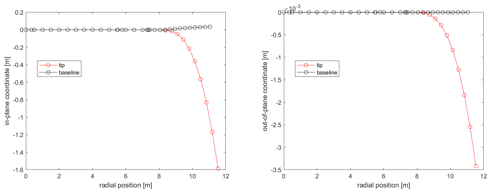
Figure 3 In-plane and out-of-plane coordinate of the centerline of the optimized tip design compared to the reference.

Figure 4 Planform of the optimized tip design compared to the reference.

Figure 5 Mass and flapwise stiffness distributions of the tip compared to the reference.

Figure 6 Internal structure of the mid-span section of the tip compared to the reference.

3 Rotating rig test setup

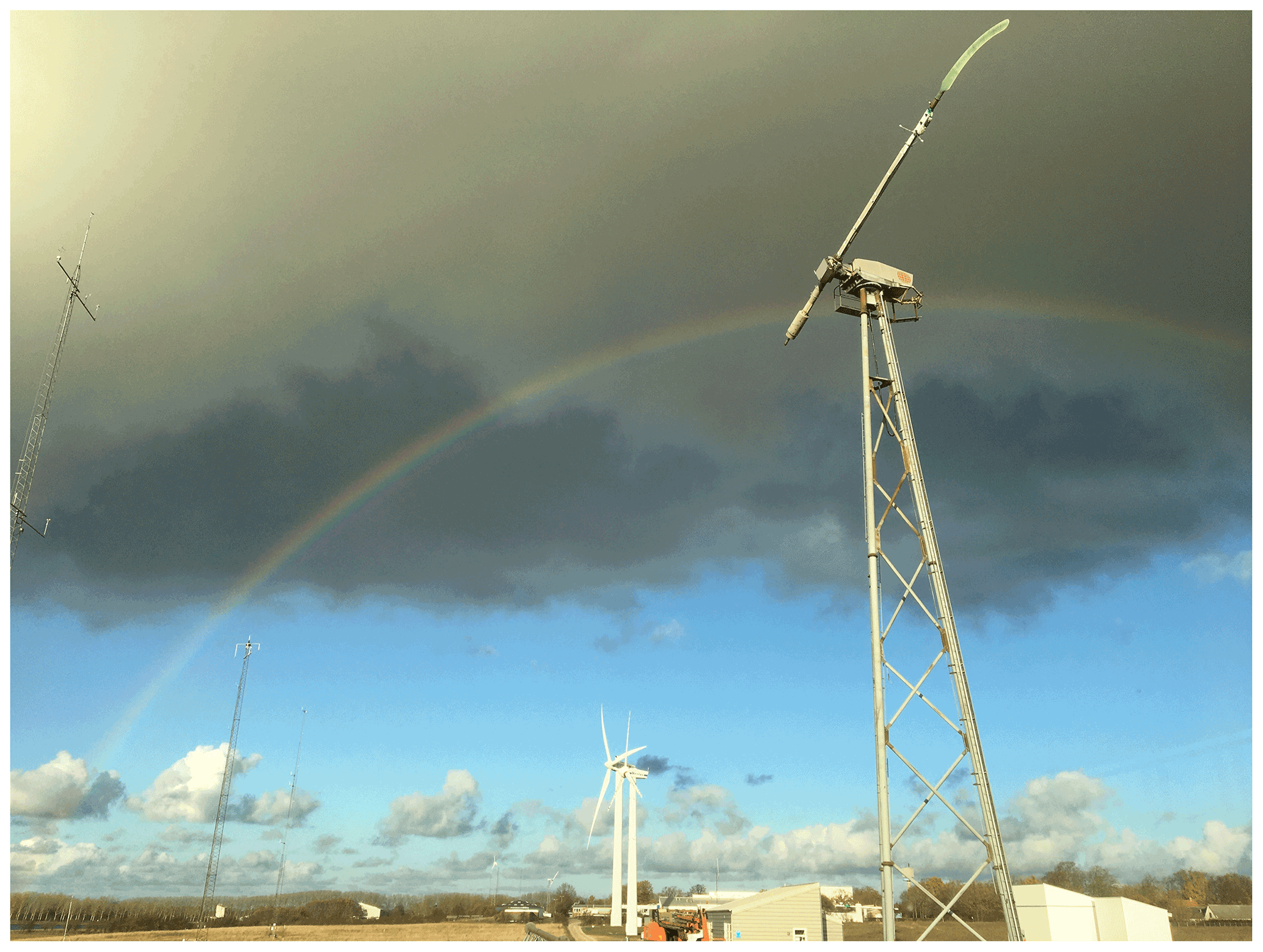
In order to fill in the gap between full-scale MW experiments and wind tunnel tests, the 95 kW Tellus turbine (Madsen and Petersen, 1990) situated at the test field at the DTU Risø campus plays an important role as a test bed for aerodynamic and aero-servo-elastic experiments (Madsen et al., 2015; Ai et al., 2019). The 5^∘ tilted rotor on the turbine has been replaced by an elastic beam, upon which different test components can be mounted on the outer part for validation of aerofoil characteristics based on pressure measurements and testing of aerodynamic sensor and control systems. Besides the main beam, a counterweight is mounted to balance the beam and the aerofoil section. During the measurements, the rotor shaft is motored and a frequency converter controls the rotational speed. The tip is mounted at the end of the boom via an adaptor (Figs. 7 and 8). The yaw angle, rotational speed, and pitch angle are controlled to defined settings and logged, together with the wind speed and direction of the nearby met mast.

Figure 7 The tip mounted on the RTR and nearby met mast.

Figure 8 The tip as seen from the boom-mounted camera.

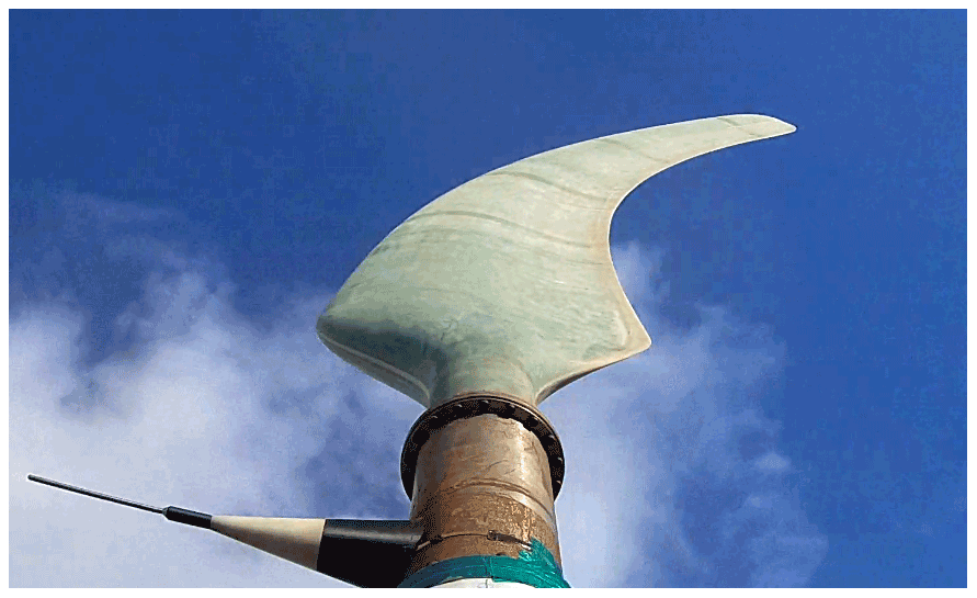
Four chordwise bands of 1 mm inner diameter pressure taps are installed on the tip at spanwise locations of 9.09, 9.79, 10.49, and 11.18 m from the boom root (15 %, 35 %, 55 %, and 75 % of the tip span, respectively). The 32 taps on each section are connected via tubing to one 1 psi and one 5 psi range DMT pressure scanners with an accuracy of 0.05 psi located on the joint piece inboard of the tip root. Sets of strain gauges are installed at the sides of the spar cap and leading edge and trailing edge at two sections at spanwise locations of 9.8 and 10.6 m from the boom root. A 6-hole Pitot tube is also mounted at the joint piece inboard of the tip root, measuring the local inflow. The data acquisition (DAQ) system is based on cRIO from National Instruments. Finally, two cameras are mounted inboard of the joint piece connected to the end of the boom.

The pressure distributions from the surface taps are numerically integrated into normal and chordwise aerodynamic forces on the local airfoil section reference frame, while an average pressure from the two nearby points is added to the trailing edge (Fig. 9). The statistics for each measurement case are processed, together with the corresponding operation settings and inflow from the met mast.

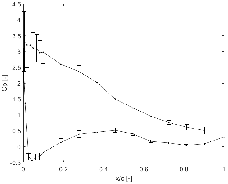
Figure 9 Example of measured average pressure coefficient at section S2 of the tip for one case at 5^∘ pitch. Error bars indicate standard deviation.

The target result is the statistical distribution of the aerodynamic forces at each section for a set of statistical distributions of operation (wind speed, yaw, pitch). The parameters of the measured 300 s cases are shown in Table 2, with the averaged values based on the pitch angle settings in Table 3. Essentially, the average results of the 16 cases are condensed into the four idealized cases, which do not necessarily represent the physics but allow for a model-to-model comparison with low influence of the specific inflow conditions.

Table 2 Parameters of all measured cases.

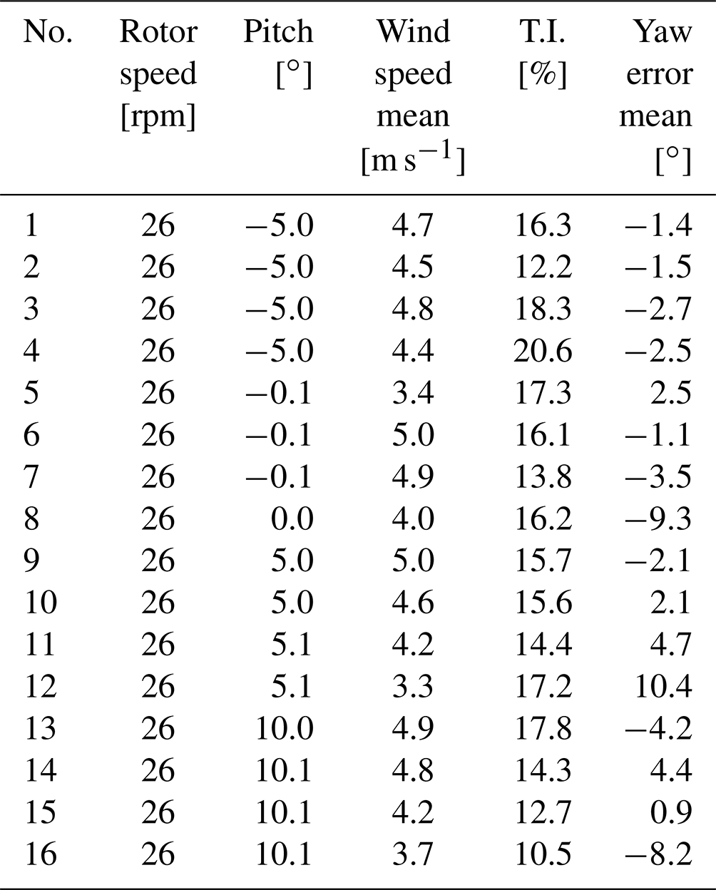
Table 3 Parameters of measured cases averaged based on pitch angle.

4 Aeroelastic simulations setup

The time domain aeroelastic simulations performed within the framework of the present study were orchestrated by the multi-body finite-element code HAWC2. All the computations shared the same structural modeling, which is described in Sect. 4.1. Several aerodynamic models were considered. In ascending order of fidelity, they are labeled in this document as:

• BEM: corresponding to a BEM formulation; implemented as a built-in capability in HAWC2 and further described in Sect. 4.2.

• NW: corresponding to a vortex-based method coupling a near-wake model with a far-wake model; implemented as a built-in capability in HAWC2 and further described in Sect. 4.3.

• LL: where the aerodynamic loading is computed with the stand-alone multi-fidelity vortex solver MIRAS and integrated into the aeroelastic solution of HAWC2 through the loosely coupled scheme described in Ramos-García et al. (2020). More details about the used aerodynamic model of MIRAS are included in Sect. 4.4.

• CFD: where the aerodynamic loads are computed with the finite-volume Navier–Stokes code EllipSys3D and integrated into the aeroelastic solution of HAWC2 through the loosely coupled scheme described in Horcas et al. (2020). Additional details of the EllipSys3D model used for the present work can be found in Sect. 4.5.

Figure 10 Distribution of aerodynamic sections along the planform.

4.1 Common structural model

All the presented methods were coupled with a common multi-body finite-element HAWC2 model. For simplicity, the tower was considered to be stiff (the maximum tower deflection is estimated to be within 10 cm, with the ratio of its first natural frequency to the rotational frequency of around 1.2). Together with the ensemble of the boom and the tip, which was considered to be a single body, the shaft and the counterweight were also modeled. The mechanical properties of the latter two components of the model are further described in Madsen and Petersen (1990). The boom and the tip were modeled by means of 32 bodies. Their mechanical properties, which are summarized in Fig. 5, were introduced as a fully populated matrix.

4.2 BEM aerodynamic model

The BEM method in the present study corresponds to the model described in Madsen et al. (2020) that is implemented in the in-house finite-element multi-body aeroelastic code HAWC2 (Larsen and Hansen, 2007). The BEM method is implemented using a polar grid approach, which is capable of modeling turbulent inflow conditions. In addition, various submodels are included to model different effects, for example dynamic inflow, yawed inflow, and unsteady 2D airfoil aerodynamics. The blade is discretized radially into 80 sections using cosine spacing, as shown in Fig. 10. Both the boom and the tip are included, while the cylindrical boom is modeled with zero lift and a drag coefficient of 0.8, as described in Sect. 2. The uniform inflow simulations were performed for 50 s with a time step size of 0.01 s. The unsteady airfoil aerodynamic model (Hansen et al., 2004; Pirrung and Gaunaa, 2018) (usually referred to as the dynamic stall model) was used for all load cases. The Prandtl tip correction described in Madsen et al. (2020) is included, which is not able to model the root vortex effect. In addition, the blade is assumed to be straight in the Prandtl tip correction, which means the impact of the blade sweep on the tip loss is not included.

4.3 Near-wake aerodynamic model

The coupled near- and far-wake model (Madsen and Rasmussen, 2004; Pirrung et al., 2014, 2016, 2017a) is a computationally efficient vortex-based method. The near wake is defined as the first quarter revolution of the trailed vortices from the own blade. It is modeled using non-expanding helical vortex filaments. The helix pitch is iterated within every time step using the indicial function approach and the steady-state induction is based on pre-calculated empirical functions that are fitted to the Biot–Savart law. The far wake is modeled using a far-wake BEM method that is without the tip-loss correction. The far-wake induction is calculated from a down-scaled thrust coefficient using a coupling factor. The near-wake induction and the far-wake induction are summed together to get the total induction. The coupling factor is calculated so that the rotor thrust is comparable to that computed with the BEM method (Andersen et al., 2010; Pirrung et al., 2016). The near-wake model was recently modified to model the blade sweep effects (Li et al., 2022), which also accounted for the curved bound vortex influence (Li et al., 2020). As for the BEM method, the unsteady airfoil aerodynamic model (Hansen et al., 2004; Pirrung and Gaunaa, 2018) is included for all load cases. As in the BEM method, the blade is discretized radially into 80 sections using cosine spacing, and the cylindrical boom is modeled with zero lift and a drag coefficient of 0.8, as described in Sect. 2. The uniform inflow simulations were performed for 50 s with a time step size of 0.01 s. Unlike the BEM method that uses the Prandtl tip correction, NW models the near-wake trailed vortices with helical vortex filaments and is able to model the root vortex effect.

4.4 Lifting-line aerodynamic model

Medium-fidelity simulations were carried out with the in-house vortex solver MIRAS (Ramos-García et al., 2016, 2017). The lifting line (LL) aerodynamic model is used in the present study in combination with a hybrid filament particle–mesh flow model (Ramos-García et al., 2019). In the LL model, the rotor blades are modeled as discrete filaments to account for the bound vortex strength and release shed and trailing vorticity into the flow. In the hybrid method, the vortex filaments are transformed into vortex particles, the vorticity of which is later on interpolated into an auxiliary Cartesian mesh. The motion of the vortex elements is determined by superposition of the free-stream velocity, the velocity induced by the blade-bound vortex, the filament wake, and the particle wake. The flow is governed by the vorticity equation obtained by taking the curl of the Navier–Stokes equation. It describes the evolution of the vorticity of a fluid particle as it moves with the flow. Moreover, MIRAS has been recently modified to accurately account for blade curvature effects (Li et al., 2020). The dynamic stall model of Øye (1994) is used to account for the stall delay related to dynamic inflow changes seen by the airfoils. The coupling between MIRAS and HAWC2 (Ramos-García et al., 2020) accounts for the wind turbine structural dynamics, a collective pitch and torque control, and the hydrodynamic loads. In a simplified manner, the coupling Python interface is in charge of transferring the blade aerodynamic loading computed by MIRAS, i.e., forces and moments at each aerodynamic section shown in Fig. 10, to HAWC2. Moreover, the kinematics of the blade computed by HAWC2, i.e., both the rigid body motion of the root and the blade axis translations and rotations at every aerodynamic section, are transferred to MIRAS via the same framework. In general, the coupling provides a common framework between the different numerical codes, paving the way for a seamless comparison. A 12Rx4Rx4R Cartesian mesh has been employed in all cases, with a constant spacing of 0.5 m in the x, y, and z directions, which adds up to a total of more than 2 million cells. The bound vortex is discretized with 80 straight segments with constant spacing. Both the boom and the tip are included in the LL model. All uniform inflow simulations have been performed for 200 s with a time step size of 0.008 s, adding up to a total of 25 000 time steps. A free boundary condition was used in all directions. Moreover, an eight-order stencil is used to spatially discretize the vorticity equation, a particle re-meshing is forced every time step to maintain a smooth field, and a periodic re-projection of the vorticity field is applied to maintain a divergence-free field.

4.5 EllipSyS3D aerodynamic model

Higher-fidelity simulations were performed with the three-dimensional computational fluid dynamics software EllipSys3D (Michelsen, 1992, 1994; Sørensen, 1995). EllipSys3D is a multi-block finite-volume code for structured grids, accounting for a wide range of modeling capabilities. In the present work, the incompressible Reynolds-Averaged Navier–Stokes (RANS) equations were solved in general curvilinear coordinates. The solution was advanced in time with a dual time stepping method using a time step of 4 ms. To accelerate the convergence of the solution, grid sequencing was used. The k–ω SST turbulence model (Menter, 1994) was selected due to its performance when dealing with airfoil flows. Two distinct sets of simulations were carried out: one assumed fully turbulent flow, while the other accounted for a correlation-based transition model (Sørensen, 2009). These two sets of computations are labeled in the present document as turb and trans, respectively.

The deflections of the boom centerline and the mounted-tip centerline, computed by HAWC2, were introduced in the CFD solution during run time. These deflections were subsequently applied to the surface grid through a spline interpolation. The surface grid deflection was then smoothed into the inner domain through a mesh-deformation algorithm based on the distance to the blade surface. Rotation was simulated by applying a rotational motion to the full computational grid as a solid body. At every time step, the CFD loading was computed and injected into the HAWC2 solution. This was done by integrating the pressure and frictional loads (including forces and moments) in a series of sectional planes which are normal to the local blade axes. The location of such sectional cuts was forced to correspond to the position of the aerodynamic sections that were defined in the rest of the methods included in this work (see Fig. 10). For more details about the EllipSys3D and HAWC2 aeroelastic coupling implementation, the reader is referred to Horcas et al. (2020).

The grid was generated in two consecutive steps. First, a structured mesh around the cylindrical boom and the tip surfaces was generated with the Parametric Geometry Library (PGL) tool (Zahle, 2019). A total of 128 cells were used in the spanwise direction, and the chordwise direction was discretized with 256 cells (with 8 of them lying on the trailing edge). Secondly, the surface mesh was radially extruded with the hyperbolic mesh generator Hypgrid (Sørensen, 1998) to create a spherical volume grid. A total of 128 cells were used in this process, and the resulting outer domain was located approximately 30 m away from the tip surface. A boundary layer clustering was taken into account, with an imposed first cell height of $\mathrm{1}\times {\mathrm{10}}^{-\mathrm{5}}$ m, in order to target y⁺ values lower than the unity. The resulting volume mesh had a total of 5.2 million cells. An inlet/outlet strategy was followed for the boundary conditions of the outer limit of the domain, and both the boom at the tip itself were modeled as walls. A sketch of the ensemble of the boundary conditions is depicted in Fig. 11, together with a visualization of the mesh.

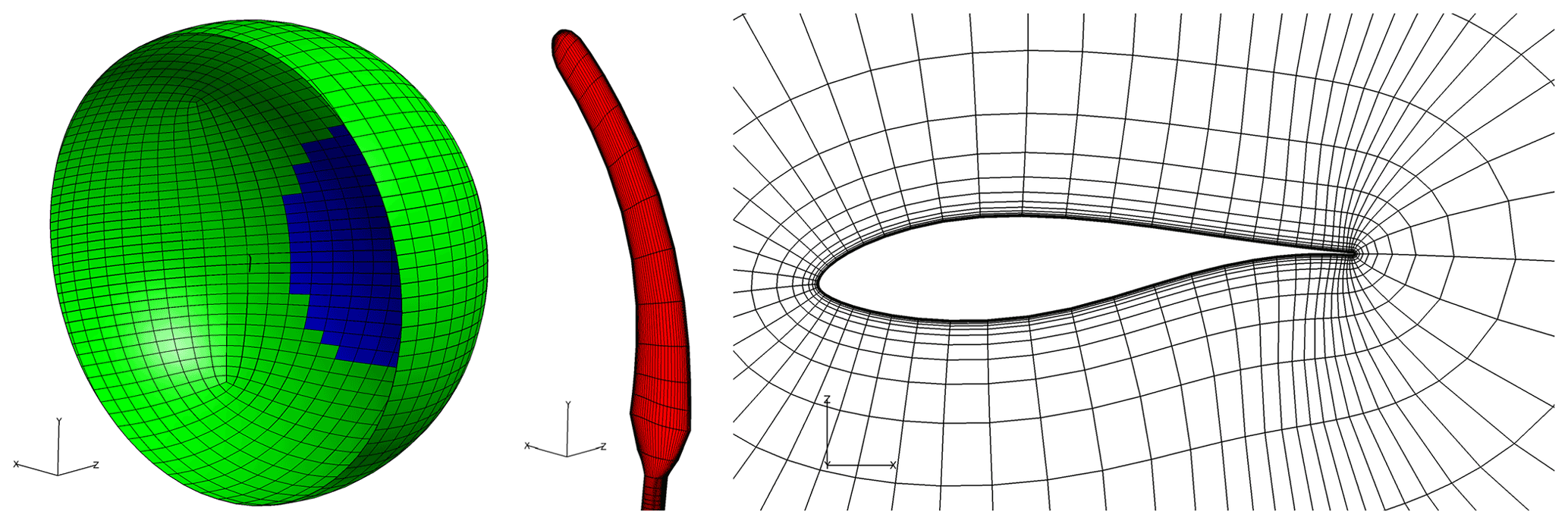
Figure 11 Visualization of the EllipSys3D mesh. For clarity, only one out of every four grid lines is shown. Left: overview of the boundary conditions distribution. Half of the spherical domain is not depicted and the freestream velocity vector is aligned with z axis. Green color corresponds to inlet and blue to outlet. Middle: detail of surface mesh around the walls, here depicted in red. Right: cross-sectional mesh around the tip at half of the projected length.

5 Comparison of test and simulation results

This section contains the comparison of measured loads with the aeroelastic loads predicted using the aerodynamic models of varying fidelity. Because no wake rake was mounted on the rotating rig, only the measured forces normal to the chord based on surface pressures are used. Insufficient wind speed measurements were available to accurately estimate shear coefficients, so no mean shear profile is present in the simulations. The effect of shear is, however, assumed to be minor, due to the small rotor diameter of the rotating test rig. All the simulations shown here use transitional polars. Since the state of the boundary layer during operation in the field is unknown, the transitional polars have been selected, since these were closer to the results. It has been shown that the comparison of fully turbulent CFD and LL using fully turbulent polars is consistent, and this is briefly demonstrated. But generally, the loading was found to be underpredicted using fully turbulent polars and fully turbulent CFD. These results are omitted here for brevity.

The section is organized as follows: in Sect. 5.1, aeroelastic simulations of all fidelity levels are compared to the mean experimental results. A comparison of sectional loads as a function of pitch angle is included and comparisons to the earlier wind tunnel tests of a scaled geometry in Barlas et al. (2021b) are made. In Sect. 5.2, the effect of turbulence on the spanwise load distribution and the distributed standard deviation of the loading is evaluated using the BEM, NW, and LL solvers.

5.1 Uniform inflow

Unless otherwise stated, the results shown here are averaged from four simulations at the four slightly different operating conditions for each pitch angle, see Table 2.

5.1.1 Spanwise load distribution

The averaged normal force from measurements and simulations and the averaged simulated chordwise force are shown in Fig. 12. Similar observations can be made for −5 and 0^∘ pitch angle (negative sign is pitch towards feather). Although the codes capture the inboard measured normal forces, there is a clear outlier at the most outboard section for the −5^∘ pitch case and a slight underprediction generally. The shape of the normal force is predicted similarly well by NW, LL, and CFD, which all predict a smaller slope than the BEM simulations. The largest difference in slope is found to be inboard, where there is a clear effect of the root vortex visible in the results of all codes except BEM. Towards the tip, the normal loading predicted by LL and NW is larger than the loading predicted by CFD, which is largely due to the smoothed chord in the CFD simulations, see Fig. 4. The CFD simulations of the chordwise force show a large peak towards the tip, which will be investigated later in this section.

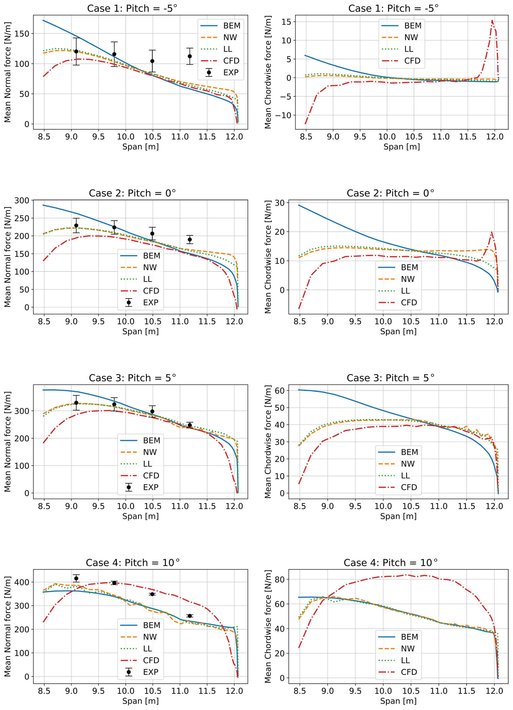
Figure 12 Comparison of normal (left panels) and chordwise (right panels) load distribution obtained from simulations and measurements. Results shown are averaged from four simulations per pitch angle, see Table 2.

At 5^∘ pitch, no peak is observed in the chordwise loading of the CFD simulations. The measured normal force agrees very well with the predictions by LL and NW. The beginning of stall is seen to lead to a less smooth load distribution of the NW simulations outboard of 10.5 m span. This is less visible in LL, possibly due to the use of a vortex core and a less fine point distribution towards the tip.

At 10^∘ pitch, shown in the last row of Fig. 12, some stall delay becomes visible in the CFD simulations and the experiment, leading to much higher normal forces than predicted by the codes that rely on airfoil data (average loads increase due to higher than maximum lift values dictated by stall delay). The NW and, to a lesser extent, LL simulations now show non-smooth force distributions along the whole span due to stalling flow. Because the operation here is close to maximum lift, at a small $\mathrm{d}{C}_{\mathrm{L}}/\mathrm{d}\mathit{\alpha }$ slope in the polars, the influence of the root vortex and tip vortex becomes much smaller in the codes using airfoil data. Therefore, the difference between BEM and LL/NW is smaller than for the lower pitch angle cases.

5.1.2 Sectional loads as a function of pitch angle

The purpose of Fig. 13 is to evaluate the predicted and measured slopes of the normal forces as a function of pitch angle. This enables the comparison of trends with the wind tunnel work in Barlas et al. (2021b). At section S1, the effect of missing root vortex in the BEM simulations is clearly visible, causing an overprediction of the loading in the linear region. This is in good agreement with the data presented in Barlas et al. (2021b). The slope in the experiment and CFD is linear up to 10^∘, while the codes using airfoil data predict the onset of stall.

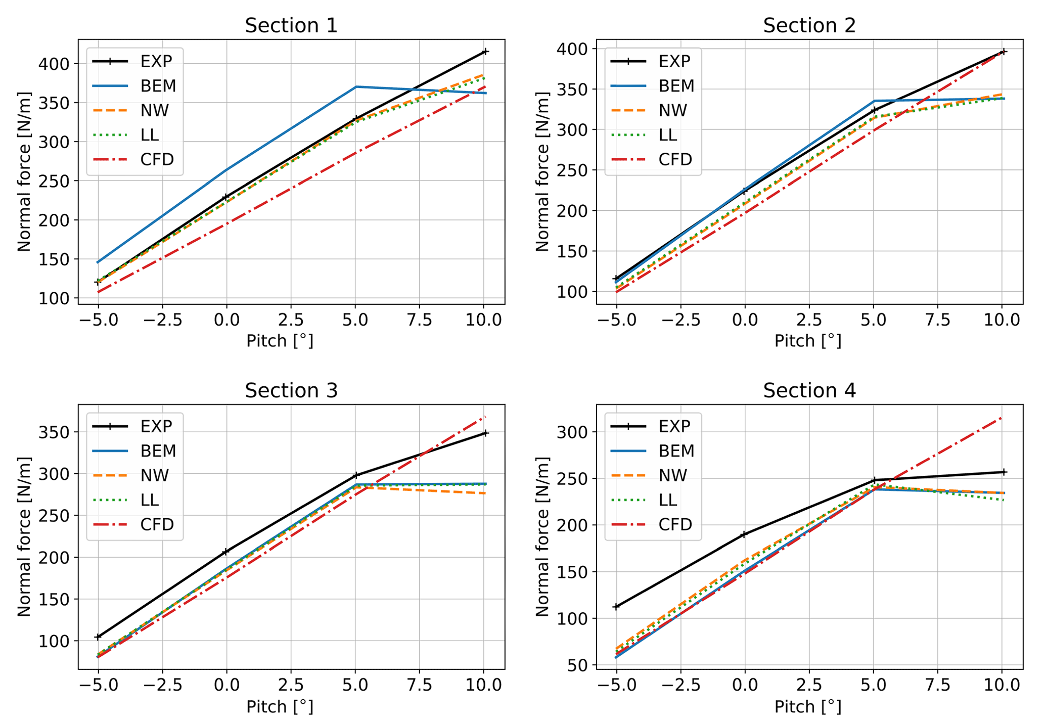
Figure 13 Comparison of normal force from simulations and experiment as a function of pitch angle. Results shown are averaged from four simulations per pitch angle, see Table 2.

At sections S2 and S3, the experiment shows indications of stall occurrence towards 10^∘. The CFD-based simulation also predicts a linear behavior, while the other codes stall too early. At sections S3 and S4, all airfoil data-based codes predict almost the same loading, while the experiment shows a lower slope than all codes in the attached flow region, especially at S4, and a clear stall at 10^∘.

The generally very good agreement between NW and LL computations in attached flow was also observed in the previous comparison with wind tunnel measurements. At section S4, the agreement is improved in the present work because the swept tip shape is taken into account by the NW model due to the modifications described briefly in Sect. 4.3. In the present campaign, the measured loads are generally higher than the predicted loads. In the wind tunnel campaign, the agreement between measurements and simulations was better, likely due to the more accurate knowledge of the inflow conditions. The better performance in stall predicted by CFD compared to the measurements and the inability of the airfoil data-based models to predict performance in stall are also consistent with the wind tunnel campaign in Barlas et al. (2021b).

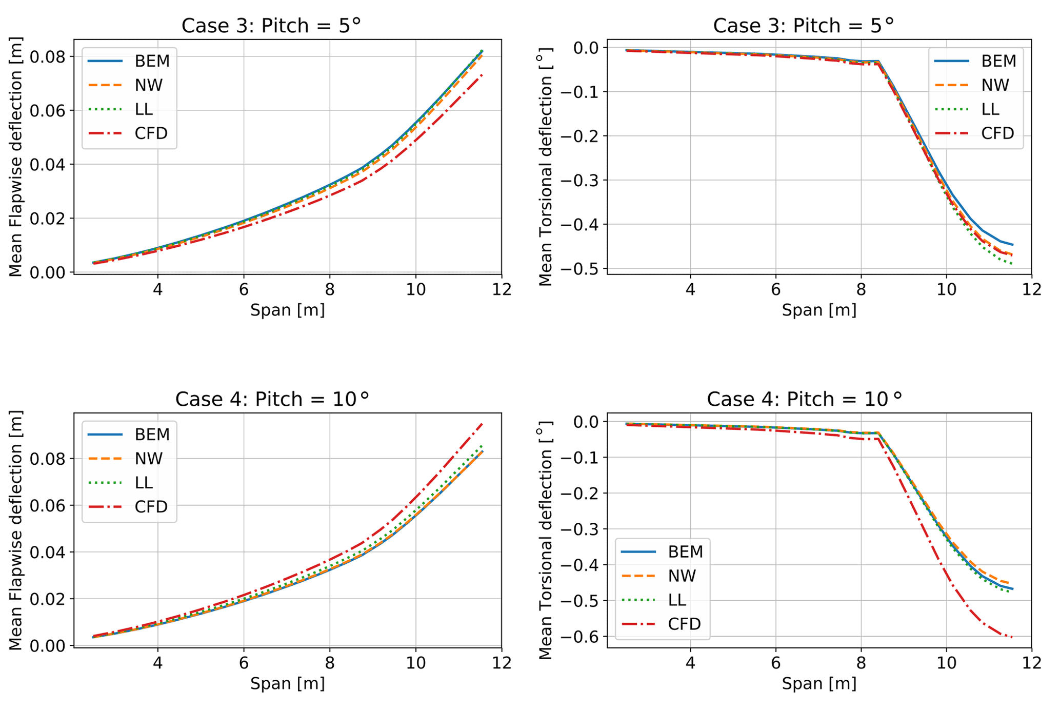
Figure 14 Comparison of mean deflections for case 3 and case 4. The torsional deflection is given about the pitch axis.

5.1.3 Deflections

The torsional and flapwise deflections for cases 3 and 4 are shown in Fig. 14. Because all aerodynamic models are coupled to the same structural solver, the very similar aerodynamic forces in case 3 (see Fig. 12) cause very similar structural deflections. In case 4, the delayed stall predicted by the CFD leads to comparably larger deflections. The deflections are generally small, but the torsional deflection will have an influence on the mean loading due to its close relationship with the angle of attack. The agreement of the predicted deflections in cases 1 and 2, the plots of which are not included here for brevity, is very similar to case 3 but at a lower overall level due to the smaller aerodynamic forcing.

Figure 15 Comparison of resultant force magnitude (left panels) and angle (right panels) between LL and CFD for cases 3, 9, and 13 from Table 2. Clearly, the spikes in chordwise force towards the tip in the CFD results shown in Fig. 12 are due to a rotation of the force.

5.1.4 Investigation of 3D flow at the very tip and transitional versus turbulent simulations

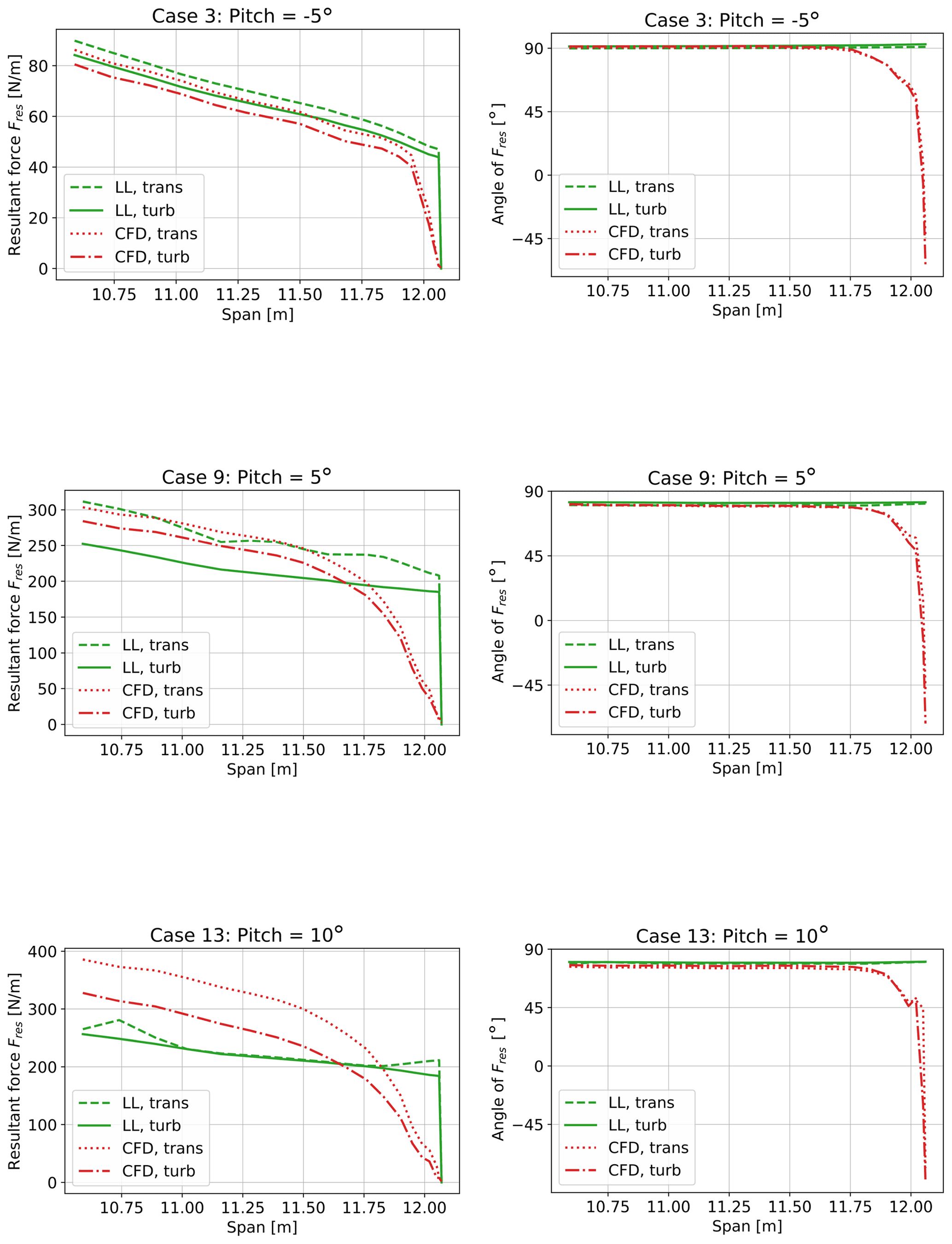
Figure 15 sheds some light on the origin of the peaks in the chordwise force distribution predicted by CFD in Fig. 12, and compares transitional and turbulent simulations. The LL results are also shown here, because they represent the highest fidelity code using airfoil data in this study. The left column shows the resultant force due to combination of the normal force and chordwise force, and the right column shows the angle of the resultant force with respect to the airfoil chord. It becomes clear that the rotation of the resultant force in the CFD results towards the tip causes the peak in the chordwise loading. This rotation is probably due to the highly three-dimensional flow at the tip, as it is illustrated in Fig. 16 for the particular case 3. Due to the lack of flow visualization during the tests, we can only rely on the CFD results to explain the 3D flow at the boom transition and tip.

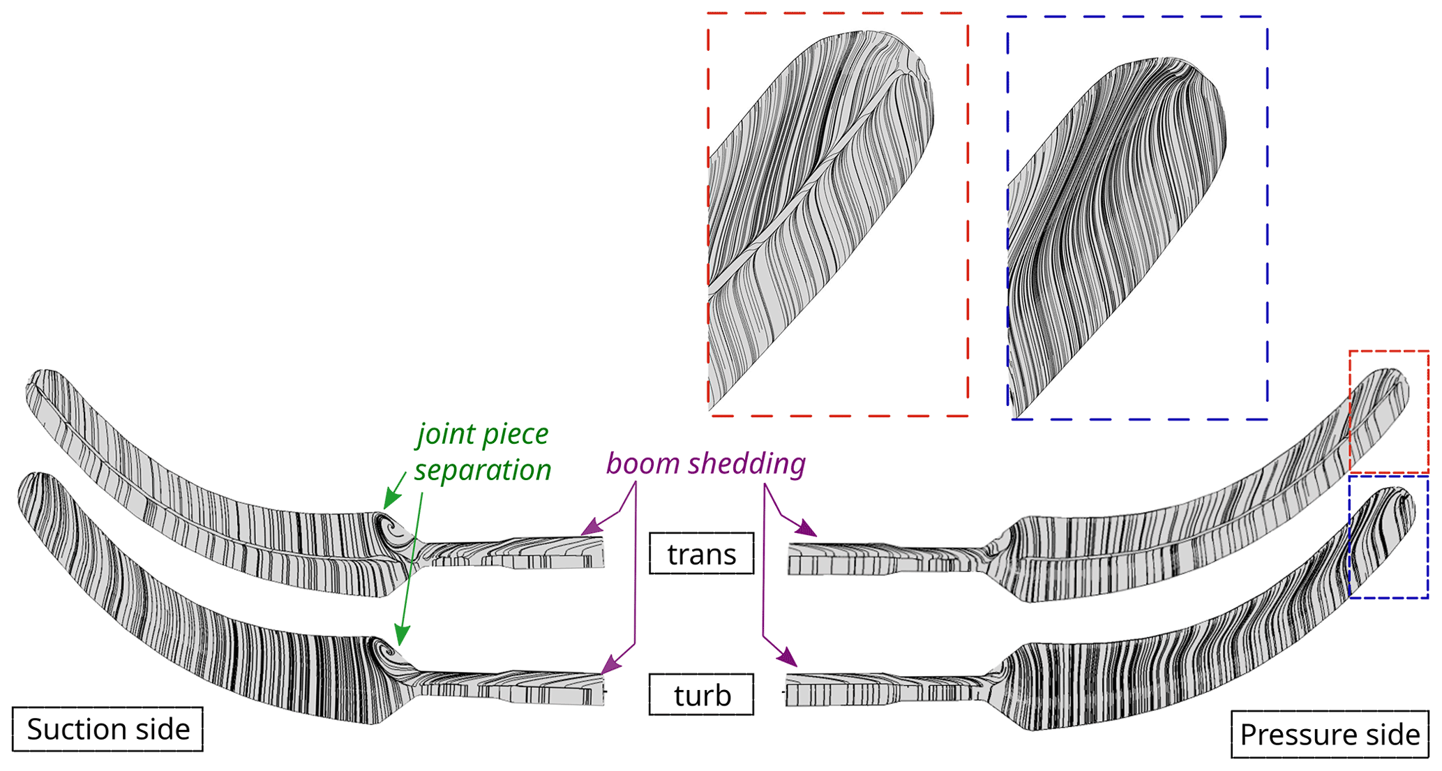
Figure 16 Surface-restricted stream lines computed with the CFD method for case 3 corresponding to a pitch of −5^∘. Both trans and turb results are presented based on the solution of the last computed time step.

LL is unable to predict the near-tip direction change of the load, and actually, these angles and forces would not be possible to achieve based on airfoil data, because there is a significant spanwise flow in the CFD simulations. Along these lines, it could be speculated that one of the factors explaining why all the other methods showed higher loading when compared to CFD could also lie in this three-dimensional behavior.

As already mentioned, there seems to be generally larger tip loss in the CFD simulations than in the LL simulations. This is in part due to the rounded tip geometry (see Fig. 4), and was a common feature for both turbulent and transition simulations. In attached flow (see case 3 in Fig. 15), the differences between laminar and turbulent profile data agree very well with the differences in the CFD simulations between transitional and fully turbulent flow. The agreement becomes worse at a pitch angle of 5^∘, where light stall is already present. At 10^∘ the flow is stalled in LL, which leads to very small differences between the transitional and turbulent simulations. In the CFD simulations, the stall is delayed and, thus, the difference between laminar and turbulent flow is much larger.

5.2 Turbulent inflow

Simulations accounting for an inflow turbulence that matches the measured one during the experimental campaign were carried out. The averaged cases based on pitch angle defined in Table 3 were numerically reproduced with three different fidelity simulations, i.e., BEM, NW, and LL. Fully resolved CFD simulations were not carried out due to the significantly high computational requirements of such cases, which were beyond the resources allocated for the present work.

First of all, the turbulence generator of Mann (1998) was used to create four turbulence boxes with an objective turbulence intensity of 15.4 %, which matches the average turbulence intensity of the four cases. Seed numbers 202, 302, 402, and 502 were used to account for different turbulence realizations. The generated boxes have a size of $\mathrm{4096}\times \mathrm{32}\times \mathrm{32}$ cells in the streamwise, vertical, and lateral directions, respectively, with a constant cell size of 2 m. The following constants were used to account for land-based turbulence generation αϵ=1.0, L=40, and γ=3.9.

Cases 1 to 3 in Table 3 have been modeled in LL, each one including a different pitch angle, wind speed, and yaw angle. Case 4 was not run with turbulence due to the high angle of attack (AoA), which causes stall and leads to issues with the NW and LL vortex solvers. All four generated turbulent boxes (four seeds) were run in each one of the LL setups, adding up to 12 simulation cases. LL simulations with and without the rotating test rig were performed, adding up to a total of 24 cases.

In MIRAS, the turbulent boxes are transformed into a particle cloud by computing the curl of the velocity field. The turbulent particles are released one diameter upstream of the rotor plane and interact freely with the turbine wake, if existent. The vortex solver accounts for turbulence development as it convects downstream towards the rotor plane. In the simulations without a turbine, the local velocities are calculated in every time step at the rotor plane position, and a 64×64 mesh with a cell size of approximately 1.5 m is used for the velocity extraction. This velocity field is loaded in the NW and BEM simulations, allowing the same turbulent structures as simulated in MIRAS to be accounted for. In this way, it is possible to closely mimic the turbulence seen by the turbine in MIRAS, although the influence of the turbine and its wake on the inflow turbulence field can not be accounted for in the lower-fidelity models.

All codes (BEM, NW, and LL) simulate each seed for 900 s at a time step of 0.01 s. The initial 100 s are discarded in the postprocessing.

In the following, the mean and standard deviation of the loads from the turbulent simulations are compared to the experimental values.

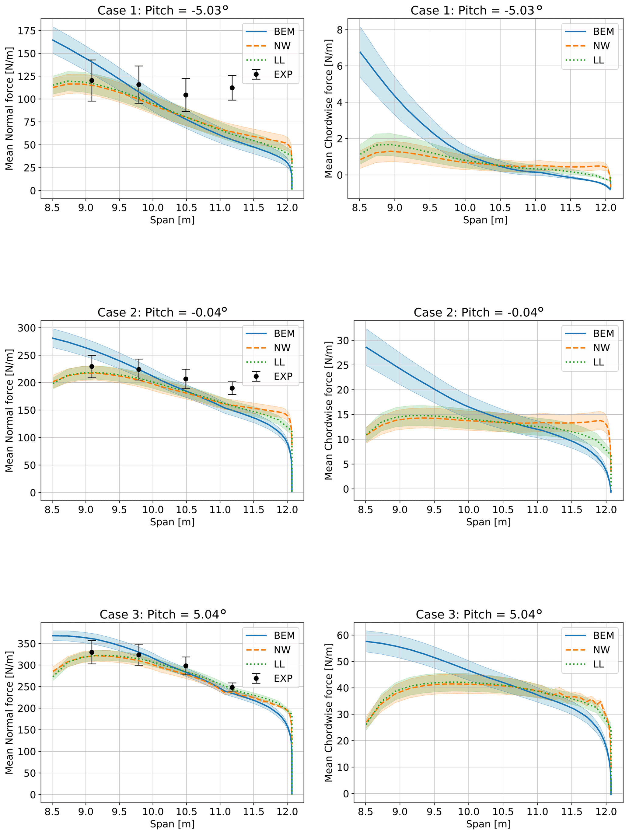
Figure 17 Comparison of normal and chordwise force from turbulent simulations and the experiment. Results shown are averaged from four turbulent seeds per pitch angle, using the mean operating conditions as shown in Table 3 up to a pitch angle of 5^∘. The shaded areas show the standard deviation between the mean values of the four simulations per pitch angle, to indicate the variability due to turbulent seed.

5.2.1 Spanwise mean loading distribution

The spanwise mean loading in the normal and chordwise directions obtained from measurements and simulations is shown in Fig. 17. The mean forces are computed as mean_seed(mean_time(F^s(t))), where the inner mean operation is performed on the time series for a given turbulent seed and the outer mean operation is performed between the turbulence seeds which are indicated by the superscript “s”.

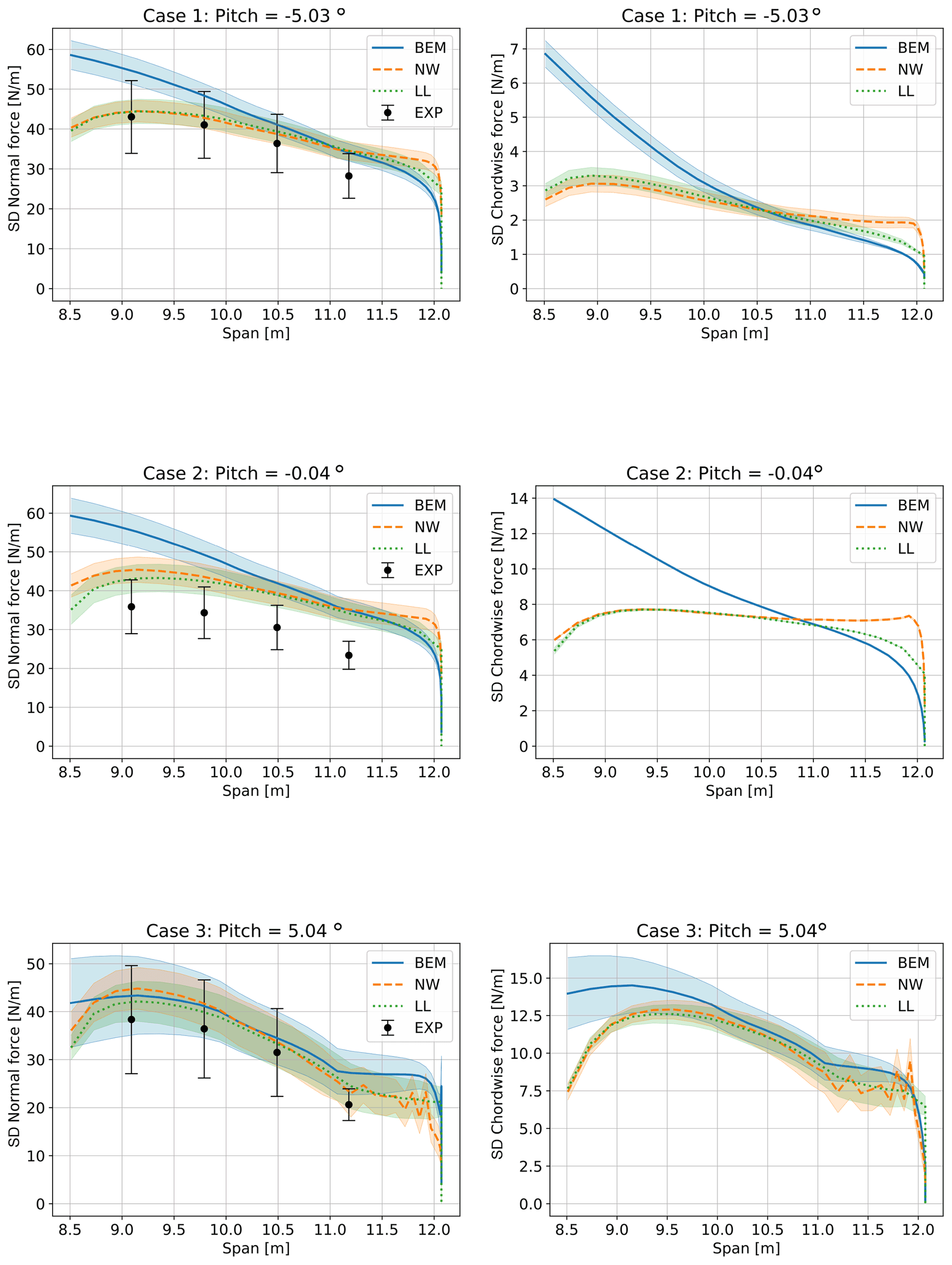
Figure 18 Comparison of standard deviations of normal force from turbulent simulations and the experiment. Results shown are averaged from four turbulent seeds per pitch angle, using the mean operating conditions as shown in Table 3 up to a pitch angle of 5^∘ The shaded areas show the standard deviation between the standard deviations of the four simulations per pitch angle, to indicate the variability due to turbulent seed.

The shaded area in Fig. 17 represents the standard deviation of the mean values of the results obtained using four different turbulence seeds: sd_seed(mean_time(F^s(t))). They have an almost constant width along the span. This shows that the different seeds lead mainly to different offsets of the mean load distribution and not to different slopes. An exception is the region towards the tip, where the shaded areas narrow, especially for the chordwise force. The error bars in the experiments represent the standard deviation of the mean values obtained from the experiment: sd_case(mean_time(F^c(t))), where the superscript “c” indicates the measurement case number. The averaged experimental values differ both in operating points (see Table 2) and in turbulent realization. Therefore, the standard deviations of the measured mean load distributions are not directly comparable to the standard deviations for the simulations, which are only due to different turbulent seeds. The observations regarding slopes of the loading and comparison to the experiment are similar to the uniform inflow cases shown in Fig. 12. The NW and LL results show excellent agreement except at the very tip, where the NW method predicts higher loading. The BEM results have a steeper slope with higher loading inboard due to the missing root vortex effect, and lower loading outboard due to the missing effect of the backward sweep on the tip loss.

Generally, the spread between the results for different turbulence seeds indicates that a large part of the deviation between experiments and simulations may be explained by variations between turbulence realizations, with an exception of the outmost section at a pitch of −5^∘.

5.2.2 Standard deviation of spanwise loading

The distribution of the standard deviations of the normal loading and chordwise loading are shown in Fig. 18. These standard deviations are computed as mean_seed(sd_time(F^s(t))), with the superscript “s” indicating a turbulence seed. The shaded area represents the standard deviation of the four standard deviations of the simulations using four turbulent seeds: sd_seed(sd_time(F^s(t))). As above, the error bars in the experiments represent the standard deviation of the mean standard deviation values obtained from the experiment: sd_case(sd_time(F^c(t))), where the respective four measured time series for the cases “c” differ in terms of both mean operating point and turbulence. This is not directly comparable to the simulations, which were performed at the mean operating conditions to reduce computational cost. Therefore, the error bars from the experiment, which include variations due to mean operating point variation and turbulence realization, are generally wider than the shaded areas from the simulations, which vary only due to turbulence.

The measured standard deviation of the normal force is generally similar to the simulated standard deviation. An exception is case 2 at roughly 0^∘ pitch, where the simulated standard deviations are about 20 % larger than the measured values. The slope of the standard deviation of the loads as a function of the span seems to be overpredicted by BEM compared to the experiment. The NW and LL results are in better agreement with the measured data. This is likely due to the dynamic modeling of the root vortex influence in the NW and LL simulations, which clearly reduces the standard deviation of the loading at the inboard part. The root vortex influence is generally more prominent in the chordwise force, because the induced vorticity causes a change in AoA that changes both the magnitude and direction of the aerodynamic forces. The magnitude affects both the normal and chordwise forces, while a change of the angle mainly leads to differences in the chordwise force. The effect of beginning separation is clearly visible in the NW simulations at 5^∘, especially close to the tip.

The shaded area, which represents the spread in standard deviations between turbulence seeds, agrees very well between LL and NW, with the BEM predicting a much larger spread in case 3 (5^∘ pitch). It is unclear why the four different seeds lead to almost exactly the same standard deviations of the chordwise force at a pitch angle of 0^∘, even though the standard deviation of the normal force varies with turbulence seed. But the effect is consistent across the model fidelities, and it was confirmed that the four seeds lead to four different time series of the chordwise loading, which happen to have almost exactly identical standard deviations.

6 Conclusions

The aeroelastic response of a swept tip is investigated for application to wind turbine tip extensions by controlled field testing in the outdoor rotating rig at the Technical University of Denmark (DTU). The swept tip shape in focus is the result of design optimization focusing on locally maximizing power performance within load constraints compared to an optimal straight tip. The tip model is instrumented with spanwise bands of pressure sensors and is tested in atmospheric inflow conditions. A range of fidelities of aerodynamic models are used to simulate the test cases and results are compared with the measurement data, namely a blade element momentum (BEM) model, a coupled near- and far-wake model (NW), a lifting-line hybrid wake model (LL), and fully resolved Navier–Stokes computational fluid dynamics (CFD) simulations. The first simulations tackled a series of idealized inflow conditions that were obtained by averaging several time windows of the experimental data. Results show that the measured mean normal loading can be captured well with the vortex-based codes and the CFD solver. The CFD solver seemed to generally underpredict the measured mean loading for these idealized conditions in attached flow. However, this higher-fidelity method computed a similar stall delay to that seen in the measurements at a high angle of attack. Similar trends to those seen in earlier wind tunnel measurements were observed when plotting the measured and simulated loading against the pitch angle. The CFD solution shows a highly three-dimensional flow at the very tip that leads to large changes in the angle of the resultant force with respect to the chord at the very outboard part of the curved tip. These angle changes cannot be predicted by any model using 2D airfoil data. No measurements were available at these outboard stations and, therefore, we were not able to validate this phenomenon with measurements. In a second stage of the analysis, the influence of turbulence on the definition of the ideal cases was addressed. Simulations with four different turbulence realizations indicated that a large part of the deviations between measured and simulated mean loading by the higher-fidelity codes can be due to seed-to-seed variations. These turbulent simulations show that the measured standard deviations of the normal force match those predicted by the vortex codes well. There are some deviations when comparing to the BEM simulations, especially towards the root section. Future work should focus on full-scale validation of aeroelastically optimized tip shapes, with focus on further enabling structural tailoring features and topologies, and possible combination with active aerodynamic add-on features.