Application of the Townsend–George theory for free shear flows to single and double wind turbine wakes – a wind tunnel study

The evolution of the mean velocity and the turbulence downstream of wind turbine wakes within the atmospheric boundary layer has been studied over the past decades, but an analytical description is still missing. One possibility to improve the comprehension of this is to look into the modeling of turbulent bluff body wakes. There, by means of the streamwise scaling of the centerline mean velocity deficit, the nature of the turbulence inside a wake can be classified. In this paper, we introduce the analytical model of classical wake theory as introduced by Albert Alan Townsend and William Kenneth George. To test the theories, data were obtained from wind tunnel experiments using hot-wire anemometry in the wakes of a single model wind turbine and a model wind turbine operating in the wake of an upstream model wind turbine. First, we test whether the requirements under which the Townsend–George theory is valid are fulfilled in the wake of a wind turbine. Based on this verification we apply the Townsend–George theory. Further, this framework allows for distinguishing between two types of turbulence, namely equilibrium and non-equilibrium turbulence. We find that the turbulence at the centerline is equilibrium turbulence and that non-equilibrium turbulence may be present at outer parts of the wake. Finally, we apply the Townsend–George theory to characterize the wind turbine wake, and we compare the results to the Jensen and the Bastankhah–Porté-Agel models. We find that the recent developments from the classical bluff body wake formalism can be used to further improve the wind turbine wake models. Particularly, the classical bluff body wake models perform better than the wind turbine wake models due to the presence of a virtual origin in the scalings, and we demonstrate the possibility of improving the wind turbine wake models by implementing this parameter. We also see how the dissipation changes across the wake, which is important to model wakes within wind farms correctly.

1 Introduction

Wind turbines are usually clustered in wind farms with the consequence that downstream turbines operate depending on the wind direction and wind speed in the turbulent wakes of upstream turbines (e.g., Barthelmie et al., 2007; Sun et al., 2020). These wakes are characterized above all by means of the mean velocity deficit that decreases in the far wake with increasing distance from the turbine. Since this velocity deficit leads to power losses of downstream turbines, knowledge of the recovery of the wind velocity is important. Therefore, over the past decades, several empirical and engineering wake models have been derived to describe a single turbine's velocity deficit; see for instance the reviews of Porté-Agel et al. (2020) and Göçmen et al. (2016). All these models find an application in the layout optimization and, once the wind farm is built, in the control mechanisms. Ideally, these models have to be simple, fast, and computationally inexpensive despite the complex flow configuration. In addition, a model describing an axisymmetric turbulent wind turbine wake from only a few fundamental and robust assumptions is still lacking. On the contrary, the axisymmetric turbulent wake of a bluff body is a canonical turbulent free shear flow which has been studied intensively during the last decades and which can be modeled by means of an analytical model. The modeling of these flows relies on the theories proposed by Townsend (1976) and George (1989), even though results have been inconclusive and even sometimes contradictory (Johansson et al., 2003). While the wake of a wind turbine does exceed the complexity of historical wake investigations of bluff bodies due to the turbine's rotation and active interaction with the background flow, the question arises as to what extent classical wake models can be applied. So far, only the power law relationship between the velocity deficit and the streamwise distance that originates from classical wake theory has been used in empirical wind turbine wake models to predict the centerline velocity recovery (cf. Porté-Agel et al., 2020).

Within the framework of turbulence, the prediction of the centerline mean velocity deficit ΔU and the wake width δ with increasing streamwise distance X of the wake-generating model are maybe the most fundamental and relevant problems that need to be solved (e.g., George, 1989)¹. Similarly to the standard engineering models derived for wind turbine wakes, the analytical model for the evolution of bluff body wakes can only be derived for the far wake. The far wake is typically identified as the part of the wake where the shear layers that evolve between the faster ambient flow and the lee of the object of investigation have met and the turbulence is fully developed. Thus, the Townsend–George theory for free shear flows allows for predicting the downstream evolution of ΔU and δ for the axisymmetric, boundary-free, turbulent wake of a bluff body sufficiently far downstream. This analytical model is based on two cornerstone assumptions regarding the turbulence evolution. The first one is the self-similar behavior of the one-point turbulence statistics. The second cornerstone assumption focuses on the energy cascade: in the Richardson–Kolmogorov phenomenology, the energy is injected on the large scales, i.e., large vortex structures, and when these vortices decay, the energy is transferred towards smaller scales, and therefore the inter-scale energy transfer is balanced by the turbulent dissipation rate ε. This cascade is therefore in equilibrium (i.e., the energy that is injected into the system on large scales is transferred completely to smaller and smaller scales until it dissipates), while the power spectral density shows the famous $E\left(f\right)\propto f^{-\mathrm{5}/\mathrm{3}}$ decay in the inertial sub-range (where f is the frequency in Hz). In this case, the dissipation rate scales as $\mathit{\epsilon }=C_{\mathit{\epsilon }}{K}_{\mathrm{c}}^{\mathrm{2}/\mathrm{3}}/L$ along the centerline with C_ε “being constant” at high Reynolds numbers². K_c denotes the centerline turbulent kinetic energy, and L denotes an integral length scale describing the energy-containing structures. C_ε being constant is therefore one of the most critical points in the theory. The scaling of the dissipation rate ε is a scaling used in many aspects of turbulence theory and in the modeling and understanding of many turbulent flows (see for example Tennekes and Lumley, 1972). As better detailed in Sect. 2, the closure provoked by this assumption leads to the standard equilibrium streamwise scalings for ΔU and δ.

Yet, in the last years, evidence has been found that some axisymmetric turbulent wakes do not follow the standard scalings of ΔU and δ. Different experimental studies and direct numerical simulations of bluff plates with both regular and irregular peripheries found that C_ε is not constant, but instead it goes as $C_{\mathit{\epsilon }}\sim R{e}_{\mathrm{G}}^m/R{e}_{\mathrm{L}}^n$ (e.g., Vassilicos, 2015; Dairay et al., 2015; Obligado et al., 2016; Nedic et al., 2013; Es-Sahli et al., 2020). Re_G is a Reynolds number that depends on the inlet conditions, and Re_L is a local, streamwise, position-dependent one (Vassilicos, 2015). The exponents n and m have been found to be very close to unity; $m=n=\mathrm{1}$ for large values of the Taylor Reynolds number Re_λ (cf. Eq. A4). For an axisymmetric wake, $R{e}_{\mathrm{G}}=\sqrt{\mathrm{\Lambda }}{U}_{\mathrm{\infty }}/\mathit{\nu }$, where Λ is the frontal area of the plate, U_∞ is the inlet velocity, and ν the kinematic viscosity of the flow. The local Reynolds number is defined as $R{e}_{\mathrm{L}}=\mathit{\delta }{u}^{\prime }/\mathit{\nu }$, where u^′ is the RMS value of the fluctuating streamwise velocity. Within these definitions, the non-equilibrium dissipation scaling can also be written as $C_{\mathit{\epsilon }}\sim R{e}_{\mathrm{G}}^{\mathrm{1}/\mathrm{2}}/R{e}_{\mathit{\lambda }}$. These anomalous non-equilibrium scalings of ΔU and δ have been reported for experiments at $X/\sqrt{\mathrm{\Lambda }}<\mathrm{50}$; therefore there is a range of interest within some wind energy applications.

This illustrates that an investigation of C_ε in the wake gives us a new tool to classify the turbulence in the wake with C_ε being constant being an indication of “standard” equilibrium turbulence with properties of homogeneous isotropic turbulence and $C_{\mathit{\epsilon }}\sim R{e}_{\mathrm{G}}^m/R{e}_{\mathrm{L}}^n$ (or equivalently $C_{\mathit{\epsilon }}\sim R{e}_{\mathrm{G}}^{\mathrm{1}/\mathrm{2}}/R{e}_{\mathit{\lambda }}$) indicating non-equilibrium turbulence with its own set of properties.

The presence of a different dissipation scaling of ε within wind turbine wakes would have important consequences regarding the modeling of wind farms and numerical simulations: many different numerical models implicitly assume the standard dissipation scalings (for more details, see Vassilicos, 2015). However, a different dissipation scaling also implies different streamwise scalings for ΔU and δ (see Sect. 2). The disregard of this point shows that we have not yet fully understood the physics underlying the simplest possible configuration in wind energy: a single turbine facing a uniform, stationary, laminar flow. Therefore, we follow a different path in this paper than the one engineering models are based on, namely the conservation of mass and momentum to describe the mean quantities. The wake of a wind turbine can only be fully understood if the turbulence evolution is properly characterized, and the presented approach can help to integrate turbulent fluctuations in the wake. Furthermore, the fact that different dissipation scalings (the dissipation being a small-scale parameter) result in different spreading properties of the wake (a large-scale parameter) shows that the turbulence cascade controls how the wake is evolving. Therefore, the initial conditions, such as the wake generator and the background flow, become important, as they ultimately control the evolution of the cascade. It is thus important to study how the dissipation scalings are affected by the inflow conditions.

In contrast to the axisymmetric turbulent wake of a bluff body, no systematic work on the turbulence decay and on the energy cascade has been made yet in the turbulent wind turbine wake. However, Okulov et al. (2015) applied the standard equilibrium bluff body wake scalings derived from the Richardson–Kolmogorov phenomenology to experimental data to justify the presence of power law decays for ΔU and δ. In addition, Stein and Kaltenbach (2019) performed a systematic study on the nature of the dissipation scaling, testing also the non-equilibrium scaling, but with neither measuring nor taking C_ε into account in the discussion. Furthermore, for the latter, the turbine studied was within a turbulent boundary layer background flow, which means that the turbulence evolution was additionally influenced by the turbulent background flow.

In this paper, we present an experimental study on the axisymmetric turbulent wake generated by a wind turbine in a wind tunnel via hot-wire anemometry. We study the wake produced by a single turbine in uniform laminar inflow. Furthermore, we also analyze the behavior of a turbine within a turbulent background: this is achieved by placing a second turbine downstream of the first one. The second turbine is tested at two different radial positions, allowing us to explore the behavior of a turbulent wake within two different, relevant configurations within a wind farm. As this work serves as a proof of the applicability of the Townsend–George theory, we do not include an investigation of the influence of an atmospheric boundary layer (ABL) profile where inflow characteristics may differ. However, it is generally assumed that the wake of a wind turbine in an ABL can be seen as a superposition between the ABL profile and the mean velocity deficit (cf. Bastankhah and Porté-Agel, 2014). This is in agreement with Neunaber et al. (2021), where the Townsend–George theory also gives good results in the case of field measurements obtained in the wake of a full-scale turbine using a lidar.

We perform a systematic study on the applicability of the Townsend–George theory to wind-turbine-generated wakes for the different incoming flows. For this, we explore the streamwise range in which the requirements are fulfilled. We also study the behavior of C_ε for this flow (i.e., whether C_ε is constant) and therefore of the scalings of ΔU and δ. By doing so, we identify the nature of the energy cascade for the different wind turbine configurations. We find that all three turbine configurations are in good agreement with the Richardson–Kolmogorov energy cascade. Furthermore, we verify that, to some extent, they also are within the conditions and hypotheses required to apply the Townsend–George theory.

In the following, we will introduce the Townsend–George theory in Sect. 2. Here, the framework and the necessary requirements to apply the theory are introduced. Also, two important engineering wake models are introduced for a comparison. Then, the setup is presented in Sect. 3.1, and the fulfillment of the requirements is investigated in Sect. 3.2. The theory is applied in Sect. 4, and the results are discussed in Sect. 5. This paper ends with a conclusion in Sect. 6.

2 Theory

2.1 Bluff body wakes

Bluff body wakes have been the object of intensive analyses for the past 60 years, and similarly to the study of wind turbine wakes, the downstream evolution of the centerline mean velocity deficit ΔU and the wake width δ are of interest.

In this work, we will follow the revisited Townsend–George theory (Dairay et al., 2015). The classical equilibrium predictions and the non-equilibrium predictions rely on the axisymmetry of turbulence wake statistics, the self-preservation of $(U_{\mathrm{\infty }}-U(X,Y\left)\right)/\mathrm{\Delta }U$ (where U(X,Y) is the streamwise mean velocity, Y is the spanwise coordinate, $\mathrm{\Delta }U=U_{\mathrm{\infty }}-U_{\mathrm{c}}$ is the centerline velocity deficit, and U_c is the streamwise centerline mean velocity), the turbulent kinetic energy K, the Reynolds shear stress R_xr, the turbulence dissipation ε, and a scaling law for the centerline turbulence dissipation that is determined by the behavior of C_ε due to $\mathit{\epsilon }=C_{\mathit{\epsilon }}{K}_{\mathrm{c}}^{\mathrm{2}/\mathrm{3}}/L$. Both sets of predictions are obtained from the Reynolds-averaged streamwise momentum and turbulent kinetic energy equations leading to a closed set of equations for ΔU(X) and the wake width δ(X).

These hypotheses also allow for expressing the momentum conservation within the wake as $(\mathit{\theta }/\mathit{\delta }{)}^{\mathrm{2}}=\mathrm{\Delta }U/U_{\mathrm{\infty }}$. The momentum thickness θ is defined by ${\mathit{\theta }}^{\mathrm{2}}=\frac{\mathrm{1}}{U_{\mathrm{\infty }}^{\mathrm{2}}}\underset{\mathrm{0}}{\overset{\mathrm{\infty }}{\int }}U(U_{\mathrm{\infty }}-U)r\mathrm{d}r$, which is constant with X, and the wake's width is characterized here by the integral wake width δ defined by ${\mathit{\delta }}^{\mathrm{2}}\left(X\right)=\frac{\mathrm{1}}{\mathrm{\Delta }U}\underset{\mathrm{0}}{\overset{\mathrm{\infty }}{\int }}(U_{\mathrm{\infty }}-U)r\mathrm{d}r$ (both quantities are linked via momentum conservation as $(\mathit{\theta }/\mathit{\delta }{)}^{\mathrm{2}}=\mathrm{\Delta }U/U_{\mathrm{\infty }}$).

The equilibrium predictions for axisymmetric turbulent wakes (see Townsend, 1976; George, 1989) for the streamwise evolution (along X) of ΔU and δ are

$$\begin{array}{}\text{(1)}& \mathrm{\Delta }U\left(X\right)=A_{\mathrm{EQ}}{U}_{\mathrm{\infty }}{\left(\left(X-X_{\mathrm{0},\mathrm{EQ}}\right)/\mathit{\theta }\right)}^{-\mathrm{2}/\mathrm{3}},\end{array}$$

$$\begin{array}{}\text{(2)}& \mathit{\delta }\left(X\right)=B_{\mathrm{EQ}}\mathit{\theta }{\left(\left(X-X_{\mathrm{0},\mathrm{EQ}}\right)/\mathit{\theta }\right)}^{\mathrm{1}/\mathrm{3}},\end{array}$$

where A and B are dimensionless constants and X₀ is a virtual origin (that appears naturally from the mathematical formulation and has to be the same for ΔU and δ).

In contrast, the non-equilibrium predictions are

$$\begin{array}{}\text{(3)}& {\displaystyle }& {\displaystyle }\mathrm{\Delta }U\left(X\right)=A_{\mathrm{NEQ}}{U}_{\mathrm{\infty }}{\left(\left(X-X_{\mathrm{0},\mathrm{NEQ}}\right)/\mathit{\theta }\right)}^{-\mathrm{1}},\text{(4)}& {\displaystyle }& {\displaystyle }\mathit{\delta }\left(X\right)=B_{\mathrm{NEQ}}\mathit{\theta }{\left(\left(X-X_{\mathrm{0},\mathrm{NEQ}}\right)/\mathit{\theta }\right)}^{\mathrm{1}/\mathrm{2}}.\end{array}$$

The only difference between equilibrium and high-Reynolds-number non-equilibrium scalings for ΔU and δ is in the scaling of the centerline value of ε: as discussed in the Introduction, the non-equilibrium turbulence dissipation law is ${\mathit{\epsilon }}_{\mathrm{c}}=C_{\mathit{\epsilon }}{K}_{\mathrm{c}}^{\mathrm{3}/\mathrm{2}}/\mathit{\delta }$, where K_c is centerline turbulent kinetic energy, ε_c is the centerline turbulence dissipation, and C_ε is a dimensionless coefficient which is constant in equilibrium turbulence but proportional to the ratio of two Reynolds numbers ($R{e}_{\mathrm{G}}^m/R{e}_{\mathrm{L}}^n$) in the case of non-equilibrium turbulence.

Another important assumption used throughout the theory is that the large scales of the turbulence are represented by the wake width δ and therefore δ∝L (Cafiero et al., 2020). This is an important and frequently overlooked assumption within the Townsend–George theory. To the authors' knowledge, it has not been verified for wind turbine wakes.

To summarize, the Townsend–George theory of axisymmetric turbulent wakes relies on the following flow properties.
Requirements to apply the Townsend–George theory.

1. The flow has to be decaying turbulence: we will focus on the range for which the turbulent kinetic energy is a decreasing function of the streamwise distance.

2. The flow has to be turbulent. A way to verify this requirement is to check that the velocity signal has

   • a.

     a large value of Re_λ (i.e., Re_λ>200) and

   • b.

     a power spectral density with an inertial sub-range that decays according to the $E\left(f\right)\propto f^{-\mathrm{5}/\mathrm{3}}$ power law.

3. The mean streamwise velocity and the turbulence quantities discussed above also have to be self-preserving and thus show a self-similar scaling (for a more detailed study on this point, we refer the reader to Dairay et al., 2015).

4. The mean velocity components and the turbulence quantities have to be axisymmetric.

5. As stated, the flow has to be in a streamwise range for which the longitudinal integral length scale is proportional to the wake width (L∝δ).

If all conditions are fulfilled, the theory predicts power law decays for the velocity deficit and the wake width. Furthermore, the exponents of such power laws can be related to the dissipation scaling of ε in the flow.

In order to disentangle the different dissipation scalings and thus identify equilibrium and non-equilibrium turbulence, two criteria have to be checked.
Criteria for equilibrium and non-equilibrium turbulence.

• i.

  Does C_ε being constant hold? In this case, no Reynolds number dependence of C_ε should be seen.
  Yes: There is equilibrium turbulence.
  No: There is indication for non-equilibrium turbulence.

• ii.

  The Taylor Reynolds number Re_λ and the local Reynolds number Re_L need to change with downstream distance in order to verify criterion (i). More specifically, Re_L has to decrease according to George (1989) in the case of non-equilibrium turbulence.

  If Re_L and Re_λ do not change, it is therefore not possible to draw conclusions on the occurrence of equilibrium and non-equilibrium turbulence, and the results are inconclusive.

In the following, we will refer to the equilibrium scaling as EQ scaling and the non-equilibrium scaling as NEQ scaling.

2.2 Wind turbine wake models

In the past, a lot of effort was put into the understanding and finding a description of the wake flow of wind turbines, especially its recovery on the centerline and the wake expansion, by carrying out experiments and simulations. Additionally, different theories have been underlain. However, an analytical model that is capable of including different inflow conditions and turbine operations does still not exist. In the following, we will briefly introduce two commonly used wake models that we will compare to the EQ and NEQ wake models.

The first model we discuss, developed by Niels Otto Jensen in 1983, is based on the conservation of momentum (cf. Jensen, 1983). It is assumed that the normalized velocity deficit is

$$\begin{array}{}\text{(5)}& {\displaystyle \frac{\mathrm{\Delta }U}{U_{\mathrm{\infty }}}}={\displaystyle \frac{U_{\mathrm{\infty }}-U_{\mathrm{W}}}{U_{\mathrm{\infty }}}},\end{array}$$

where the wake velocity U_W is top hat shaped and evolves with increasing downstream distance X according to

$$\begin{array}{}\text{(6)}& {\displaystyle \frac{\mathrm{\Delta }U}{U_{\mathrm{\infty }}}}=\left(\mathrm{1}-\sqrt{\mathrm{1}-c_{\mathrm{T}}}\right)\cdot {\left(\mathrm{1}+{\displaystyle \frac{\mathrm{2}{k}_{\mathrm{J}}X}{D}}\right)}^{-\mathrm{2}},\end{array}$$

where U_∞ denotes the unperturbed inflow velocity; U_W denotes the streamwise wake velocity; c_T denotes the turbine's thrust coefficient; D denotes the turbine's diameter; and k_J denotes the wake expansion, which is assumed to be constant. While Jensen suggests k_J=0.1, k_J=0.075 is suggested in Barthelmie et al. (2006).

A more recent model that includes the conservation of mass in addition to the conservation of momentum is the one derived by Bastankhah and Porté-Agel (2014). Here, the recovery of the centerline velocity deficit is combined with a Gaussian velocity profile:

$$\begin{array}{}\text{(7)}& \begin{array}{rl}{\displaystyle \frac{\mathrm{\Delta }U}{U_{\mathrm{\infty }}}}& =\underset{\mathrm{centerline}\mathrm{velocity}\mathrm{deficit}}{\underbrace{\left(\mathrm{1}-\sqrt{\mathrm{1}-{\displaystyle \frac{c_{\mathrm{T}}}{\mathrm{8}{\left(k_{\mathrm{BP}}\cdot X/D+\mathrm{0.2}\sqrt{\mathit{\beta }}\right)}^{\mathrm{2}}}}}\right)}}\\ & \cdot \underset{\mathrm{Gaussian}\mathrm{velocity}\mathrm{profile}}{\underbrace{\exp \left(-{\displaystyle \frac{{\left(\left(Z-Z_{\mathrm{h}}\right)/D\right)}^{\mathrm{2}}+(Y/D{)}^{\mathrm{2}}}{\mathrm{2}{\left(k_{\mathrm{BP}}\cdot X/D+\mathrm{0.2}\sqrt{\mathit{\beta }}\right)}^{\mathrm{2}}}}\right)}}.\end{array}\end{array}$$

In this formula, Y and Z denote the spanwise and wall-normal coordinates; Z_h denotes the hub height; and k_BP is the wake growth rate that needs to be specified and is on the order of magnitude of 0.03±0.02 (Bastankhah and Porté-Agel, 2014; Okulov et al., 2015). β is given by the following equation:

$$\begin{array}{}\text{(8)}& \mathit{\beta }={\displaystyle \frac{\mathrm{1}+\sqrt{\mathrm{1}-c_{\mathrm{T}}}}{\mathrm{2}\sqrt{\mathrm{1}-c_{\mathrm{T}}}}}.\end{array}$$

In the following, we will call this wake model the BP model.

It can be seen that the two approaches that were presented above to describe the wind turbine wake differ significantly from the classical wake models that were derived from the perspective of turbulence.

3 Experimental setup and verification of requirements

3.1 Setup

In the following, the experimental setup used to carry out the experiments evaluated in this study is introduced.

The experiments have been performed in Oldenburg's Large Wind Tunnel (OLWiT) at the University of Oldenburg that has an inlet of 3 m ×3 m and a closed test section of 30 m length (cf. Kröger et al., 2018). In the empty test section, the background turbulence intensity of the flow is TI=0.3 % (where $\mathrm{TI}=u^{\prime }/U$), and velocities of up to 42 m s⁻¹ can be reached. A closed-loop control keeps the velocity constant, and to correct for changes, the flow temperature, the ambient pressure, and the humidity are constantly monitored. During all experiments presented here, the uniform inlet velocity was $U_{\mathrm{\infty }}=(\mathrm{7.55}\pm \mathrm{0.05})$ m s⁻¹.

Two three-bladed horizontal-axis model wind turbines of the same type have been used in the experiments (cf. Schottler et al., 2018). In the following, they will be referred to as turbine 1 and turbine 2. Both turbines have a rotor diameter of D=58 cm and a hub height of h=72 cm (resulting in an inlet Reynolds number of $R{e}_{\mathrm{G}}=\mathrm{3}\times {\mathrm{10}}^{\mathrm{5}}$ based on the square root of the rotor surface). The rotor load is controlled using a closed-loop control to ensure a performance of the turbine at the optimal tip speed ratio of TSR≈5.8 in the full-load range (cf. Petrović et al., 2018; Neunaber, 2019). This is achieved be measuring the rotor torque and adapting it to achieve the optimal rotational speed that can be taken from a lookup table. The thrust coefficient of the whole turbine was measured by placing the turbines on a force balance, and it is $c_{\mathrm{T},\mathrm{t}\mathrm{1}}\approx \mathrm{1}$ for turbine 1 and $c_{\mathrm{T},\mathrm{t}\mathrm{2}}\approx \mathrm{1.07}$ for turbine 2 (see Neunaber, 2019). The thrust coefficient of the tower and the nacelle were also measured and yield $c_{\mathrm{T},\mathrm{n}}\approx \mathrm{0.12}$ so that the turbine operates close to the ideal thrust coefficient of $c_{\mathrm{T},\mathrm{id}}=\mathrm{8}/\mathrm{9}$ derived from the Betz limit.

As shown in Fig. 1, an array of six one-dimensional hot-wire probes with sensor lengths of 1.25 mm and a sensor diameter of 5 µm was used to measure the wake downstream of three different wind turbine array configurations at the hub height with a very high downstream resolution of $\mathrm{\Delta }X/D=\mathrm{0.17}$. The data were collected using a StreamLine 9091N0102 frame with 91C10 CTA (constant temperature anemometry) modules. A temperature correction, as proposed by Hultmark and Smits (2010), was applied to the data. At each position, 1.2×10⁶ data points were collected with a sampling frequency of f_s=15 kHz. A hardware low-pass filter with a cutoff frequency of 10 kHz has been used.

Figure 1 Setup (modified from Neunaber, 2019): a hot-wire array is used to measure the wakes of (1) a single turbine (plot color: dark purple), (2) a turbine exposed to the wake of an upstream turbine (plot color: turquoise), and (3) the half-wake of an upstream turbine (plot color: green).

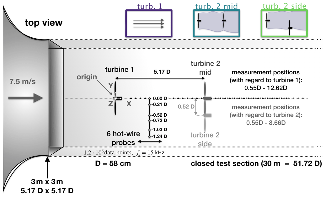
Three wake configurations were investigated (cf. Fig. 1):

1. The wake of turbine 1 is exposed to the uniform, laminar inflow in the range between $X/D=\mathrm{0.55}$ and $X/D=\mathrm{12.62}$. This configuration will be referred to as turbine 1. Based on the rotor, the blockage of the wind tunnel is 3 % in this configuration.

2. The wake of turbine 2 is positioned 5.17 D downstream in the wake of turbine 1 between $X/D=\mathrm{0.55}$ and $X/D=\mathrm{8.66}$ with respect to turbine 2³.

   • a.

     First, turbine 2 is exposed to the wake of turbine 1. Both are aligned and therefore share the centerline axis. As shown in Neunaber (2019), the inflow is thus turbulent with an average inflow velocity of 3.4 m s⁻¹ (2.1 m s⁻¹ in the center, 5.5 m s⁻¹ at the blade tip). This configuration will be referred to as turbine 2 mid.

   • b.

     Then, turbine 2 is moved 0.5 D to the side so that it is exposed to an inhomogeneous half-wake inflow. As shown in Neunaber et al. (2020), the inflow is thus turbulent and intermittent. The average inflow velocity is 5.1 m s⁻¹ with a gradient from 2.1 m s⁻¹ at one side of the rotor to 7.4 m s⁻¹ at the other side of the rotor. This configuration will be referred to as turbine 2 side.

In the cases of turbine 1 and turbine 2 mid, we measure one-half of the wake because the wake is expected to be axisymmetric in uniform inflow (Stevens and Meneveau, 2017). The horizontal position of the hot-wire array is not changed in the case of turbine 2 side so that the full wake is measured in this case.

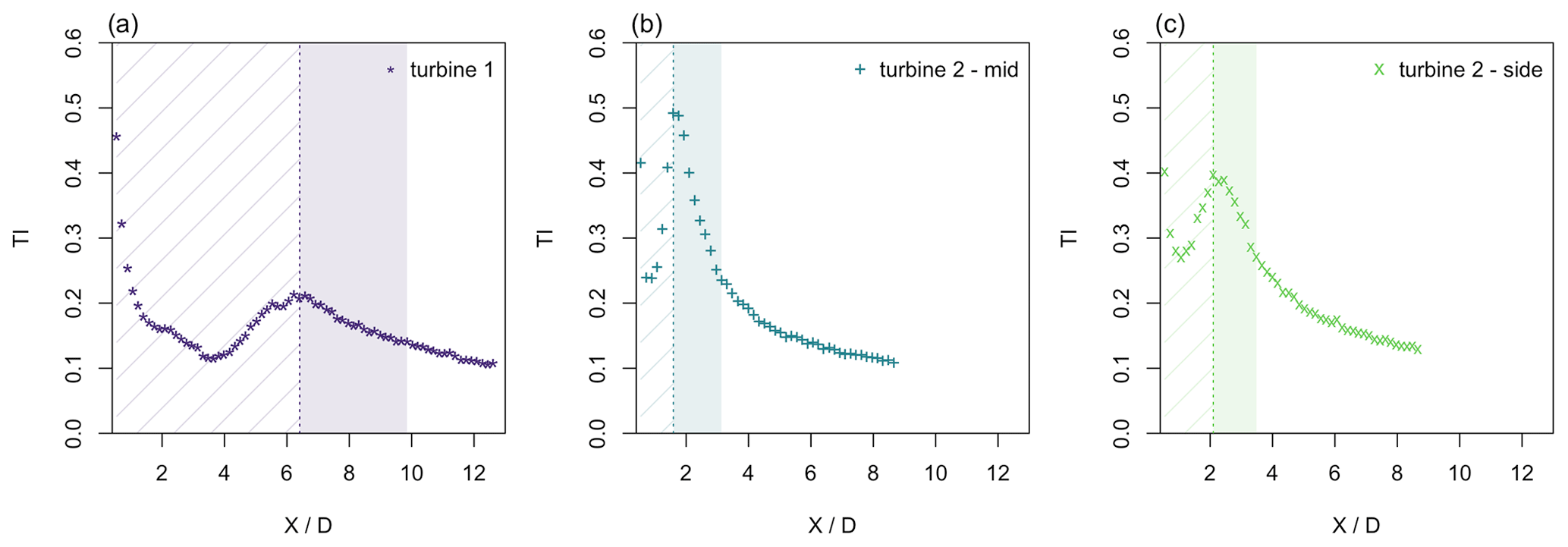
Figure 2 Centerline turbulence intensity TI for the three different inflow conditions: (a) turbine 1 – laminar inflow, (b) turbine 2 mid – turbulent, and (c) turbine 2 side – turbulent and intermittent. The vertical lines mark the maximum of the TI ($X/D=\mathrm{6.24}$ for turbine 1, $X/D=\mathrm{1.79}$ for turbine 2 mid, and $X/D=\mathrm{2.45}$ for turbine 2 side); the hatched regions upstream of the turbulence intensity maximum mark the regions that will be omitted in the following; and the colored area marks the region where the Taylor Reynolds number is changing (cf. Fig. 3).

3.2 Verification of the requirements

As explained in Sect. 2, certain requirements have to be fulfilled to justify the use of the Townsend–George theory. Therefore, in the following, we will verify that the listed criteria are accomplished.

3.2.1 Turbulence intensity

In Fig. 2, the centerline evolution of the turbulence intensity is plotted for the three inflow scenarios. As also discussed in Neunaber et al. (2020), the turbulence intensity first decreases in the nacelle's lee, then increases when the turbulence builds up due to the expansion of the shear layers evolving between the faster ambient flow and the slower wake and afterwards decreases in the far wake where the turbulence decays. The first requirement that has to be fulfilled in order to apply the Townsend–George theory is fully developed, decaying turbulence which is indicated by a decreasing turbulence intensity. Therefore, the data points in the near wake prior to the local maximum of the turbulence intensity will be masked in the following. In the plots, this is indicated by hatched areas.

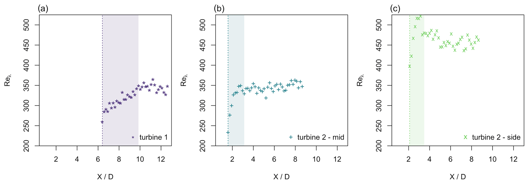
Figure 3 Downstream evolution of the Taylor Reynolds number Re_λ for the three different inflow conditions at the centerline in the decay region of the TI: (a) turbine 1 – laminar inflow, (b) turbine 2 mid – turbulent, and (c) turbine 2 side – turbulent and intermittent. The vertical lines mark the maximum of the TI, and the colored area marks the region where the Taylor Reynolds number is changing.

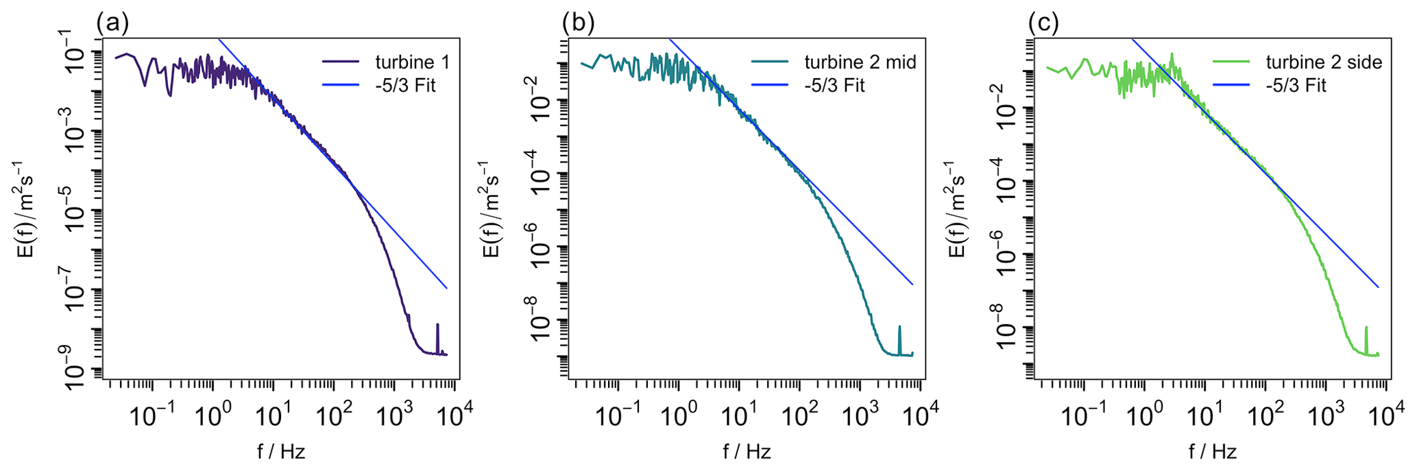
Figure 4 Energy spectral density E(f) over frequency f at the maximum turbulence intensity ($X/D=\mathrm{6.24}$ for turbine 1, $X/D=\mathrm{1.79}$ for turbine 2 mid, and $X/D=\mathrm{2.45}$ for turbine 2 side) for the three different inflow conditions: (a) turbine 1 – laminar inflow, (b) turbine 2 mid – turbulent, and (c) turbine 2 side – turbulent and intermittent. In blue, the $E\left(f\right)\propto f^{-\mathrm{5}/\mathrm{3}}$ decay is marked.

3.2.2 Taylor Reynolds number

In order to apply the Townsend–George theory, we are looking for a region with fully developed turbulence where Re_λ>200 holds, as stated in requirement 2a. In Appendix A, the calculation of Re_λ is detailed in Eqs. (A2)–(A4). In Fig. 3, Re_λ is therefore plotted in the downstream region where the turbulence intensity decays. Therefore, this requirement of the Townsend–George theory is fulfilled.

3.2.3 Energy spectral density

Next, the energy spectral density has to be checked. It is important to have an energy spectrum with a clear inertial sub-range that decays according to a power law, as explained in requirement 2b. In Fig. 4, the energy spectral density is plotted for the three inflow scenarios at the respective maximum of the turbulence intensity. Clearly, an inertial sub-range that decays according to $E\left(f\right)\propto f^{-\mathrm{5}/\mathrm{3}}$ is present in all three wake scenarios. In Neunaber et al. (2020), it is also shown how the energy spectral density has an inertial sub-range decaying with $E\left(f\right)\propto f^{-\mathrm{5}/\mathrm{3}}$ for all positions farther downstream. Therefore, the next criterion is fulfilled in the chosen downstream region.

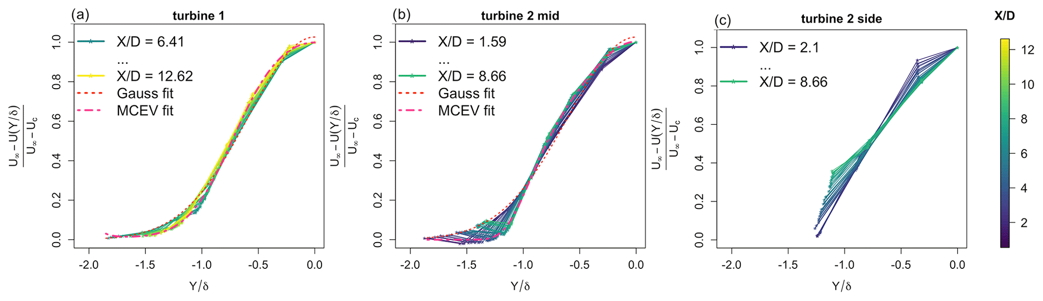
Figure 5 Plot of the wake deficit over the normalized spanwise position $Y/\mathit{\delta }$ for the three different inflow conditions: (a) turbine 1 – laminar inflow, (b) turbine 2 mid – turbulent inflow, (c) turbine 2 side – turbulent and intermittent inflow. Only curves in the decay region of the turbulence intensity are included, and the downstream position is indicated by means of the color map.

3.2.4 Self-similarity

As the Townsend–George theory originates in classical bluff body wake analysis, another important assumption is that of the self-similarity of the wake, as stated in requirement 3. To verify the self-similarity in this study, the normalized velocity deficit $\frac{U_{\mathrm{\infty }}-U(X,Y/\mathit{\delta })}{U_{\mathrm{\infty }}-U_{\mathrm{c}}}$ is plotted over the normalized radial component $Y/\mathit{\delta }$. In the case of a self-similar behavior of the turbulence, the curves are expected to collapse. For the two cases of turbine 1 and turbine 2 mid (cf. Fig. 5a and b) the curves collapse as required, and thus, a self-similar behavior is confirmed. To show that the profiles collapse to a Gaussian curve as often implied when assuming a constant eddy viscosity, a fit according to

$$\begin{array}{}\text{(9)}& {\displaystyle \frac{U_{\mathrm{\infty }}-U(X,Y/\mathit{\delta })}{U_{\mathrm{\infty }}-U_{\mathrm{c}}}}=a\cdot \exp \left(-b\cdot (Y/\mathit{\delta }{)}^{\mathrm{2}}\right)\end{array}$$

was applied. In addition, the following modified constant eddy viscosity (MCEV) model discussed in Cafiero et al. (2020) was applied:

$$\begin{array}{}\text{(10)}& \begin{array}{rl}{\displaystyle \frac{U_{\mathrm{\infty }}-U(X,Y/\mathit{\delta })}{U_{\mathrm{\infty }}-U_{\mathrm{c}}}}& =a\cdot \exp \left(-b\cdot (Y/\mathit{\delta }{)}^{\mathrm{2}}-c\cdot (Y/\mathit{\delta }{)}^{\mathrm{4}}\right.\\ & \left.-d\cdot (Y/\mathit{\delta }{)}^{\mathrm{6}}\right).\end{array}\end{array}$$

With root mean square (RMS) errors of 0.013 and 0.027 for turbine 1 and 2 mid, respectively, the MCEV model performs indeed better than the Gaussian fit with RMS errors of 0.033 and 0.054, respectively. In the asymmetric, more complex wake of turbine 2 side (cf. Fig. 5c), a self-similar behavior can not be found, and therefore, we do not expect the Townsend–George theory to fully hold there.

As we present results obtained from 1 d hot-wire anemometry, the test for self-similarity is restricted here to the mean velocity profile. However, Stein and Kaltenbach (2019) did investigate the self-similarity of the added Reynolds stress tensor components and the added turbulent kinetic energy in the wake of a model wind turbine exposed to an ABL profile. We assume therefore that this requirement also holds here.

3.2.5 Axisymmetry

In addition to self-similarity, also axisymmetry of the wake is required, as explained in requirement 4. As the measurements that we present have been carried out in one-half of the wake, we are not able to directly verify the axisymmetry. However, based on the symmetric setups for turbine 1 and turbine 2 mid and other studies with similar conditions (see, e.g., Stevens and Meneveau, 2017), we conclude that the requirement of axisymmetry can be taken as valid for these inflow conditions.

It should be noted that the axisymmetry may be influenced by the presence of the ground and an ABL profile when investigating the wake of a wind turbine in the field. However, as the mean far wake evolving downstream a turbine exposed to an ABL inflow is often described as the superposition of an ABL profile with an axisymmetric wake, it can be assumed that the requirement also holds for these cases (Bastankhah and Porté-Agel, 2014; Stein and Kaltenbach, 2019).

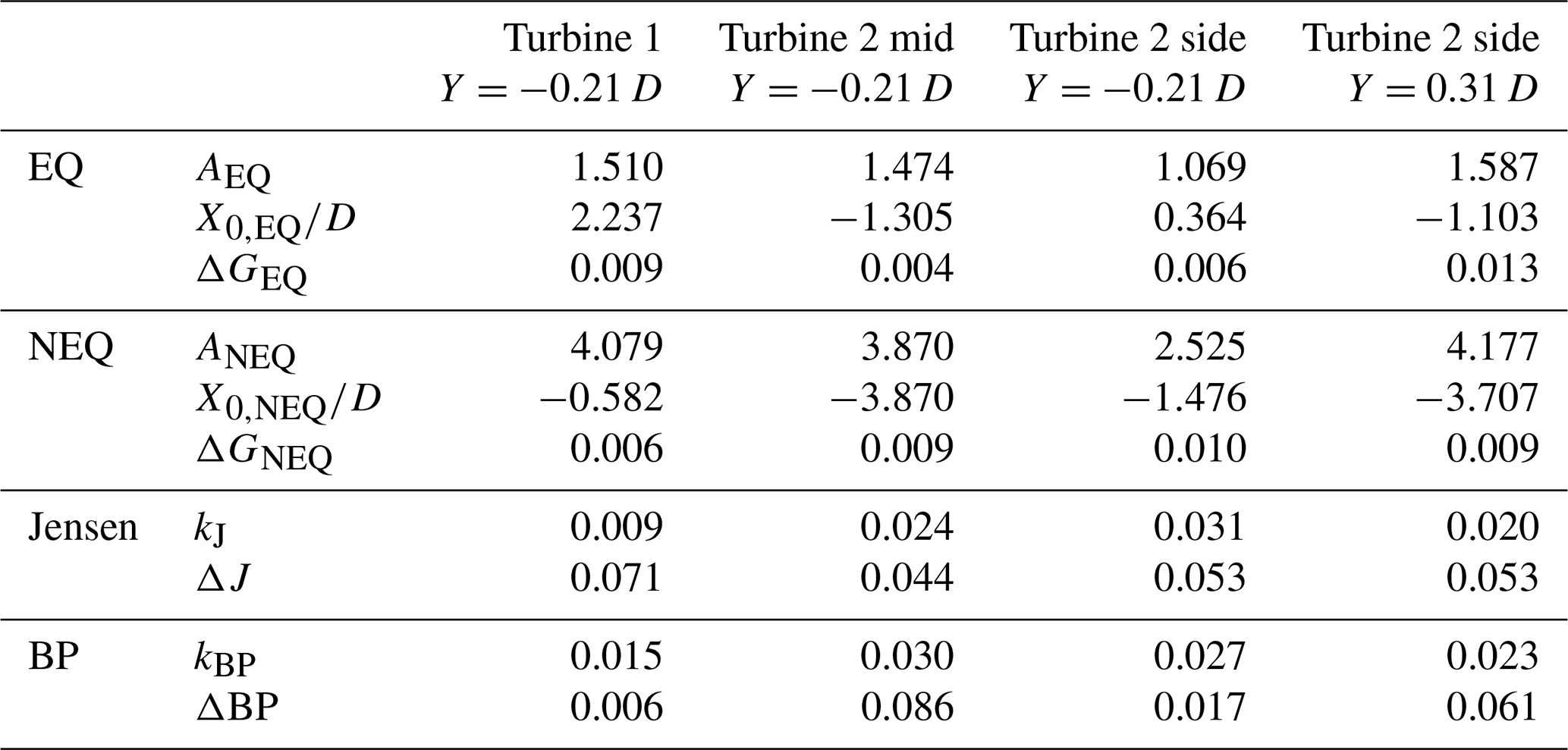
3.2.6 Integral length scale over wake width

The last requirement that needs to be fulfilled is the behavior of $L/\mathit{\delta }$; see requirement 5. As explained above, δ∝L is assumed in the Townsend–George theory for bluff body wakes. In Fig. 6, $L/\mathit{\delta }$ is therefore plotted over $X/D$ for the three scenarios, and error bars are included. The errors for $L/\mathit{\delta }$ were calculated using error propagation. As the calculation of L is quite sensitive, the error bars are rather large. Downstream of turbine 1 and turbine 2 mid, $L/\mathit{\delta }$ increases in the colored region where Re_λ changes, and it is approximately constant in the far wake. This shows how the wake turbulence has a tendency to develop towards symmetry. In the far wake, the data points are quite shattered because the integral length scale fluctuates in this region, especially downstream of turbine 2 where L tends to fluctuate due to the turbulent background inflow (for the evolution of L, see Neunaber et al., 2020, and Neunaber, 2019). Downstream of turbine 2 side in the complex inflow, the points are scattered, and an increase of $L/\mathit{\delta }$ is visible, but far downstream, $L/\mathit{\delta }$ appears to tend to a constant value. This indicates that despite the highly complex, sheared, and asymmetric inflow the turbulence appears to drive the evolution of the wake towards symmetry. A deeper analysis of this will be visited in future work. Briefly, we can conclude that the condition $L/\mathit{\delta }$ is approximately constant is fulfilled in the far wake case of turbine 1 and turbine 2 mid but not in the case of turbine 2 side.

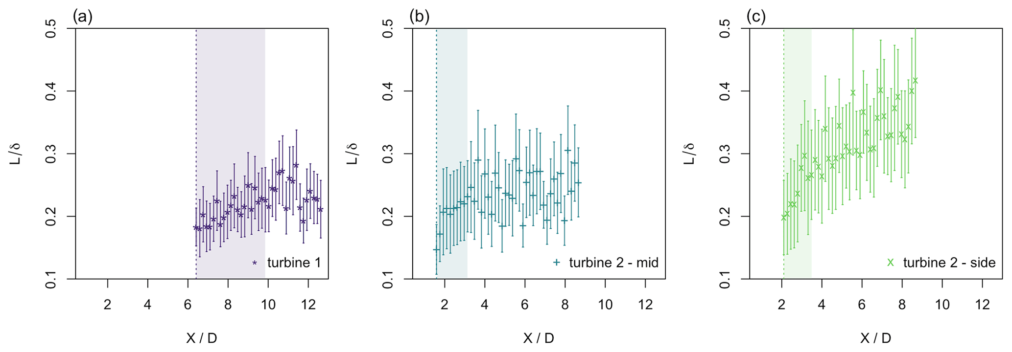
Figure 6 Downstream evolution of $L/\mathit{\delta }$ for the three different inflow conditions: (a) turbine 1 – laminar inflow, (b) turbine 2 mid – turbulent, and (c) turbine 2 side – turbulent and intermittent. The vertical lines mark the maximum of the TI, and the colored area marks the region where the Taylor Reynolds number is changing.

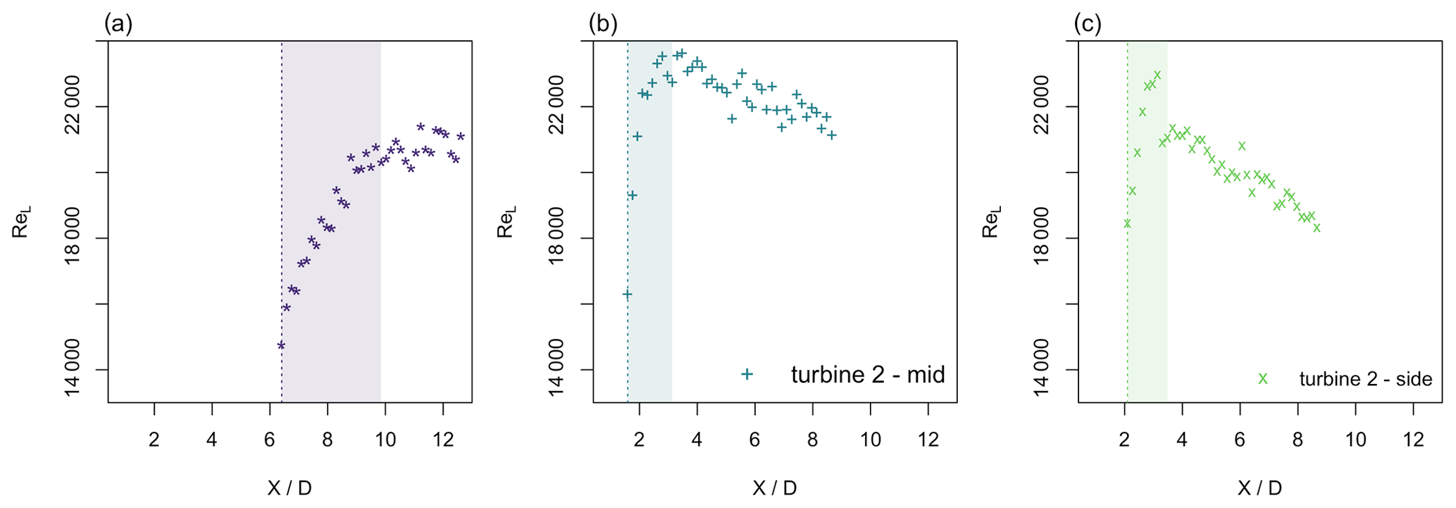
Figure 7 Downstream evolution of the local Reynolds number Re_L for the three different inflow conditions at the centerline in the decay region of the TI: (a) turbine 1 – laminar inflow, (b) turbine 2 mid – turbulent, and (c) turbine 2 side – turbulent and intermittent. The vertical lines mark the maximum of the TI, and the colored area marks the region where the Taylor Reynolds number is changing.

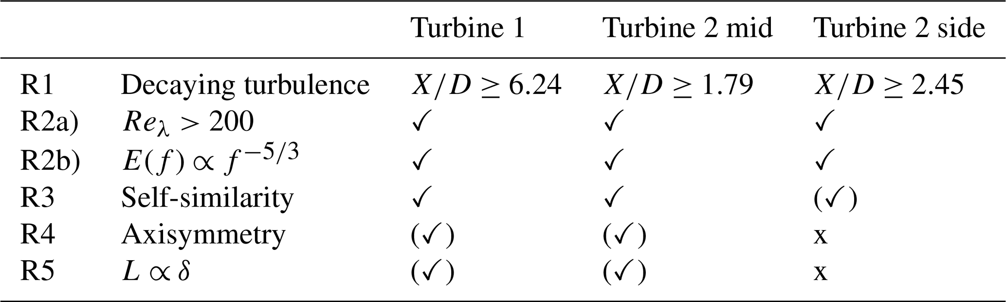
Summary of Sect. 3.2

In order to fulfill the first requirement of the Townsend–George theory, we first chose the downstream regions in which the turbulence intensity is decaying. In this region, the other requirements have been tested, and by means of the Taylor Reynolds number, the energy spectral density, the self-similarity and, particularly in the far wake, also the behavior of $L/\mathit{\delta }$, we can conclude that the Townsend–George theory can be applied to the wakes downstream of turbine 1 and turbine 2 mid. In the wake of turbine 2 side, the requirements are partially fulfilled (fully developed turbulence that is indicated by the decaying turbulence intensity, the high Taylor Reynolds numbers, and a decay of the energy spectral density has been verified, while self-similarity, axisymmetry, and $L/\mathit{\delta }$ being approximately constant are not given). Table 1 summarizes this again. With the confirmation that the requirements are met for turbine 1 and turbine 2 mid and partially for turbine 2 side, we will apply the Townsend–George theory to the data.

Table 1 Summary of the investigation of which requirements are fulfilled at the centerline in the three wake scenarios: ✓ denotes the fulfillment of a criterion; (✓) denotes the sufficient fulfillment of a criterion; and x denotes that the criterion is not fulfilled.

4 Results

After verifying the requirements that need to be fulfilled in order to apply the Townsend–George theory, the next step is to check whether non-equilibrium turbulence is present at the centerline. For this, we will first discuss the behavior of Re_λ and Re_L, and afterwards, C_ε will be investigated.

As stated above, the Taylor Reynolds number is supposed to change so that the presence of equilibrium and non-equilibrium turbulence can be disentangled. In Fig. 3, it can be seen that Re_λ changes in the region directly downstream of the local maximum turbulence intensity that was identified as the decay region in Neunaber et al. (2020) but then remains constant in the far wake. Therefore, non-equilibrium turbulence could be present in the region just after the turbulence intensity peak that is underlain in color ($\mathrm{6.24}\le X/D\le \mathrm{9.86}$ for turbine 1, $\mathrm{1.79}\le X/D\le \mathrm{3.14}$ for turbine 2 mid, and $\mathrm{2.45}\le X/D\le \mathrm{3.48}$ for turbine 2 side). We remark that Re_λ is increasing in the region of interest, and while there is no specification in the Townsend–George theory of how Re_λ has to change, George (1989) writes that Re_L has to decrease. Therefore, we also show the downstream evolution of the local Reynolds number Re_L in Fig. 7. It can be seen that Re_L increases in the marked region where Re_λ is also increasing. Farther downstream, Re_L is constant downstream of turbine 1, and it decreases downstream of turbine 2 mid and turbine 2 side. Since Re_λ remains constant in the far wake where Re_L is decreasing, the results regarding the existence of non-equilibrium turbulence are inconclusive in that range. The results also suggest that we capture the onset of the streamwise decay of Re_L and Re_λ, in agreement with the theoretical prediction.

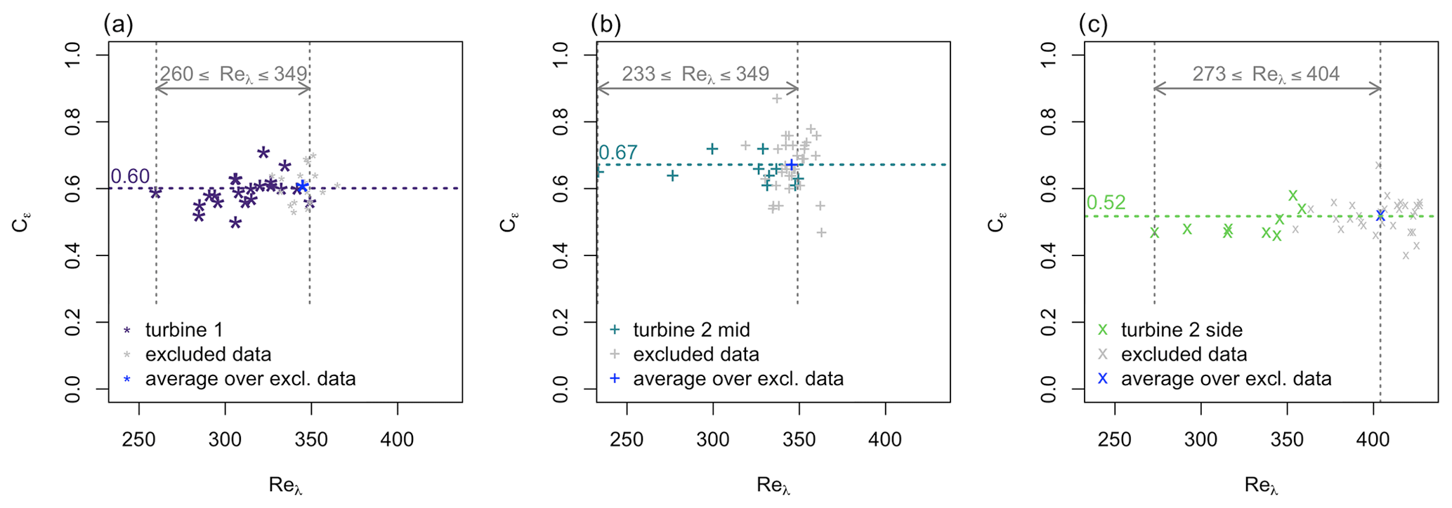
Figure 8 C_ε(Re_λ) at the centerline for the three different inflow conditions: (a) turbine 1 – laminar inflow, (b) turbine 2 mid – turbulent, and (c) turbine 2 side – turbulent and intermittent. In grey, data points within the downstream region where Re_λ does not change are masked, and their mean value is plotted in blue.

The next step is to additionally verify whether there is a dependence of C_ε on the Taylor Reynolds number in order to differentiate between the equilibrium scaling and the non-equilibrium scaling. In Fig. 8, C_ε(Re_λ) is therefore plotted for the three inflow conditions in the range where the turbulence intensity is decaying. C_ε is calculated according to Eq. (A5) in Appendix A. The data points in the downstream region where Re_λ is changing are plotted in color, while the data points in the downstream region where Re_λ is approximately constant are masked in grey, and the average over all masked points is plotted in blue. It can be seen that while the values for C_ε scatter about ±15 % around the mean value, which is normal due to the sensitivity of the calculation of C_ε, no clear dependency of C_ε(Re_λ) is present. Since this would be expected in the case of non-equilibrium turbulence, together with the inconclusive results from the investigation of Re_λ and Re_L, we can conclude that equilibrium turbulence occurs and that we do not find evidence of non-equilibrium turbulence in any of the inflow scenarios in the evaluated region in the wake of a wind turbine.

It can also be seen that the three different wakes have a different average C_ε. This indicates inhomogeneity of the dissipation constant of the turbulence inside of a wind farm. Another consequence is that the dissipation may be instationary: when the wind direction changes, the wake of an upstream turbine may pass over a downstream turbine with the consequence that C_ε in the inflow changes, e.g., from the wake to the ABL inflow. In such a scenario C_ε changes with time.

These consequences show the importance of the analysis of C_ε in the wake of a wind turbine, since computational fluid dynamics models normally rely on a constant dissipation coefficient.

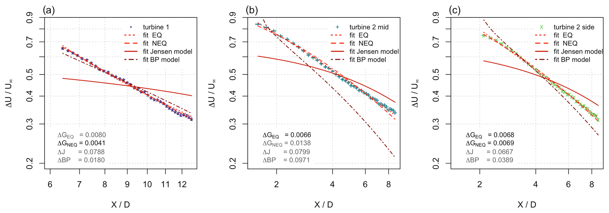
Figure 9 $\mathrm{\Delta }U/U_{\mathrm{\infty }}$ for three different inflow conditions: (a) turbine 1 – laminar inflow, (b) turbine 2 mid – turbulent, and (c) turbine 2 side – turbulent and intermittent. Error bars are included but very small. Different models are fitted to the recovery region, and the residual standard errors are presented. Note that the axes are logarithmic.

After verifying all requirements and testing for the occurrence of non-equilibrium turbulence, finally, Fig. 9 shows the downstream evolution of the normalized velocity deficit $\mathrm{\Delta }U/U_{\mathrm{\infty }}$ over $X/D$ at the centerline for all inflow conditions. An error for the velocity deficit has been calculated from error propagation, where the error of U(X) comes from the calibration uncertainty and the error of U_∞ is a statistical estimation of the inflow variation. The error bars are included in the plot, but the error bars are very small, with the maximum relative errors being 0.0054 in the case of turbine 1, 0.0035 in the case of turbine 2 mid, and 0.0043 in the case of turbine 2 side. In the following, we apply the EQ and NEQ scalings from the Townsend–George theory to the data without any preference. In addition, the two introduced wind turbine wake models, namely the Jensen model and the BP model, are fitted to the data. Here, we simplify the fitting of the EQ and NEQ scalings by using $\mathrm{\Delta }U=A_{\mathrm{EQ}}\cdot (X-X_{\mathrm{0},\mathrm{EQ}}{)}^{-\mathrm{2}/\mathrm{3}}$ and $\mathrm{\Delta }U=A_{\mathrm{NEQ}}\cdot (X-X_{\mathrm{0},\mathrm{NEQ}}{)}^{-\mathrm{1}}$, where A and X₀ are fitted. For the Jensen and the BP models, the wake expansions k_J and k_BP are used as fit variables. The residual standard errors of the respective fits are given in the legends in Fig. 9. The fit parameters can be found in Table 2. Note that we do not apply superposition wake models for the wakes of turbine 2 mid and turbine 2 side here but treat the wakes individually because we are interested in the difference a turbulent inflow has on the fit. With the hypothesis that a final universal turbulence state can be reached within a wind farm where multiple wakes are overlapping, the modeling of these multiple wake scenarios is not a question of superposition but rather of how and where this final turbulence state is reached. Regarding this line of thinking, the investigation of the individual wakes is thus of interest.

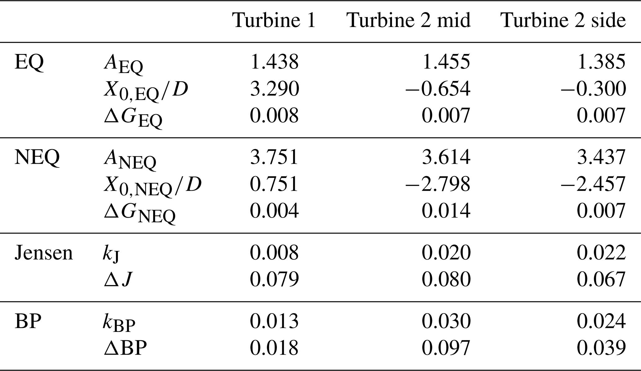
Table 2 Fit parameters and RMS errors for the different models predicting the evolution of $\mathrm{\Delta }U/U_{\mathrm{\infty }}$ for the three scenarios at the centerline.

In the case of turbine 1, the NEQ wake model and the EQ wake model predict a similar evolution of the mean centerline velocity deficit and show the best results based on the residual standard error. As the maximum error for this data set is $\partial \mathrm{\Delta }U/U_{\mathrm{\infty }}=\mathrm{0.0054}$, we can conclude that they perform similarly. The BP wake model performs less well, and it can be seen that there are deviations in the evolution of the normalized velocity deficit. The Jensen model does not capture the evolution of the mean centerline velocity deficit. It should be noted that, since the Jensen model uses a top-hat-shaped wake to calculate the average wake velocity, it was never designed to accurately model the centerline velocity deficit. To give a specific example of the consequence of making an error in the estimation of the mean velocity, we will look at the BP model: in the beginning, the velocity deficit is underestimated by 10 %, and at the end of the measurement range, the velocity deficit is overestimated by 3 %. This would lead to a difference in the power estimation of 25 % or 10 %, respectively, based on the centerline velocity for this specific wake scenario.

Downstream of turbine 2 mid, it can be seen that the EQ model captures the evolution of the velocity deficit best. The NEQ model performs less well and shows slight deviations from the data. In a systematic way, the model overestimates the velocity up to $X/D\approx \mathrm{2.5}$, underestimates the velocity in the range $\mathrm{2.5}\le X/D\le \mathrm{6}$, and overestimates it from $X/D\approx \mathrm{6}$. In the far wake, the velocity is overestimated by 3 %, which would result in an overprediction of the power of approximately 9 % for this specific wake scenario. The fits for the Jensen and the BP model show large deviations.

Downstream of turbine 2 side, the EQ and NEQ models perform best and fit the measurement points well. The Jensen model does not capture the evolution of the mean centerline velocity deficit. The BP model is not suitable for this wake condition with complex inflow, and the deviations are significant: at the end of the measurement range, the velocity is overestimated by approximately 6 %, which leads to an overestimation of the power by approximately 17 %.

Overall, it is obvious from the presented results that the EQ wake model performs well for all three wake scenarios, and in combination with the result from above that C_ε is approximately constant (cf. Fig. 8), we conclude that the EQ model from classical wake theory is a wake that performs quite well. Note that the EQ model clearly improves the mentioned engineering models.

5 Discussion

In this work, we have introduced a different approach to model the wakes of wind turbines that originates in the theory of bluff body wakes. For this, we verified first that the requirements necessary to apply these theories are fulfilled (see requirements 1–5). Then, we searched for turbulence with non-equilibrium scaling by investigating the evolution of C_ε. While we did not find evidence for non-equilibrium turbulence, we could show that both the EQ and the NEQ bluff body wake theories fit the wind turbine wake remarkably well. While it is hard to disentangle the difference in the power law exponents from the EQ and NEQ models (in the end, they are both similar in the limited streamwise range studied), we show that they both predict a functional form that properly fits our data: a power law with a non-zero virtual origin. Although the power law approach is not new to the description of the mean velocity deficit (see, e.g., Porté-Agel et al., 2020), we add new physical aspects to the use, as the formulas used here are derived from certain assumptions, and we test the requirements needed to apply the theory before using it.

To further expand the discussion of the turbulence present in the wake of a wind turbine, we did calculate C_ε for all measurement positions in the three wake scenarios in the regions where the energy spectral density shows an inertial sub-range with a power law decay. The results are presented as interpolated contour plots in Fig. 10 for the three wake scenarios. In addition, the positions of the blade tips are marked as horizontal red dashed lines, and the position of turbine 2 is marked as a vertical red dashed line in the wake of turbine 1. For all wakes, C_ε does not show strong variations inside the wake. At the centerline downstream of turbine 1 and turbine 2 mid, C_ε is larger than around the blade tip position. Downstream of turbine 2 side, the variations of C_ε inside the wake are even less pronounced, and the value is smaller than that mentioned above. The variation of C_ε due to the inflow turbulence means that different dissipation scalings are present inside a wind farm as already discussed in Sect. 4, and during a change of the wind direction, even a temporal fluctuation of the dissipation scalings can occur. Another very interesting effect is visible at some points in these plots: at the wake edges at the turbulent–non-turbulent interface between the wake and the laminar inflow, C_ε is significantly higher than inside the wake. While the data presented here are not sufficient to draw conclusions, we suspect that this may indicate a large C_ε ring surrounding the wake, similar to the ring of high intermittency that was found to surround the wake in Schottler et al. (2018) and that was shown to be traceable along the whole measured range in Neunaber et al. (2020). However, further investigation on this topic is needed to confirm this. This shows that beside the wake core that is characterized by equilibrium turbulence (indicated by C_ε being approximately constant around the centerline), there are distinctive regions with non-trivial turbulence that can be found in the wake of a wind turbine. One consequence of the variation of C_ε in the wake is that the dissipation changes radially. Even with the complex inflow of turbine 2 side that is also exposed to this C_ε ring, the wake center shows equilibrium turbulence. This confirms again the finding that the turbine creates its own dominant type of turbulence (Neunaber et al., 2020).

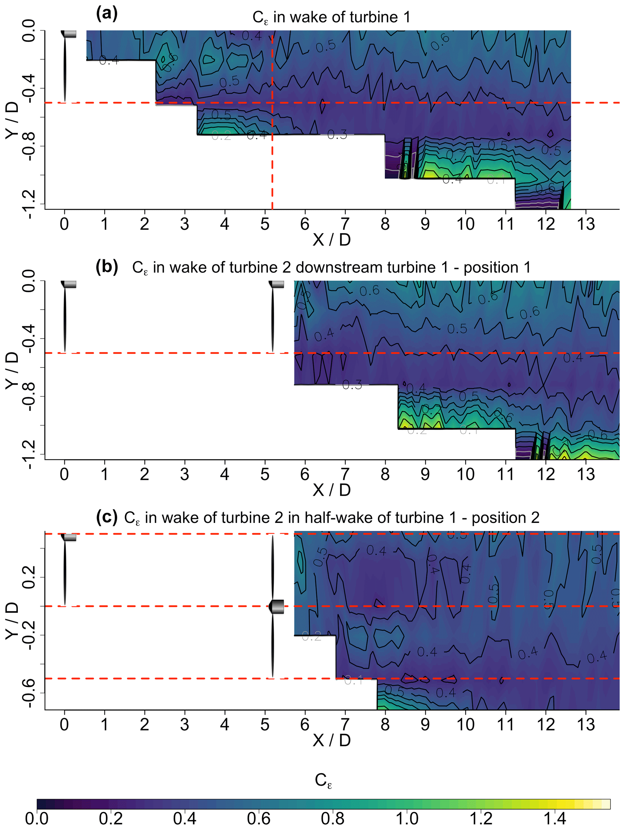
Figure 10 Interpolated surface plot of the downstream evolution of C_ε for the three different inflow conditions: (a) turbine 1 – laminar inflow, (b) turbine 2 mid – turbulent, and (c) turbine 2 side – turbulent and intermittent. Outside of the turbulent wake, C_ε is masked.

With the knowledge that the wake core is characterized by equilibrium turbulence, we also applied the different wake models to the evolution of the velocity deficit at another radial position in the wake core at $Y/D=-\mathrm{0.21}$. For the BP model, we only use the centerline velocity deficit part of Eq. (7). The results are presented in Fig. 11 for the three wake scenarios, and the coefficients are given in Table 3. The plots include error bars that are obtained similarly to the errors in Fig. 9, and the maximum errors are 0.0062 for turbine 1, 0.0077 for turbine 2 mid, 0.0066 for turbine 2 side, and in addition 0.0055 for turbine 2 side at $Y/D=\mathrm{0.31}$. It can be seen that all wake models except the Jensen model perform very well in the case of turbine 1. With respect to the errors, the NEQ and BP models perform similarly, and the EQ model shows a slightly worse fit. The Jensen model does not capture the evolution of the centerline velocity deficit, which is expected, as it was developed to estimate wake losses for the whole wake. In the case of turbine 2 mid, the EQ model performs best, and the NEQ shows slight systematic differences, as discussed above. Both the BP and the Jensen model do not capture the evolution centerline velocity deficit, but the Jensen model performs reasonably well in the far wake.

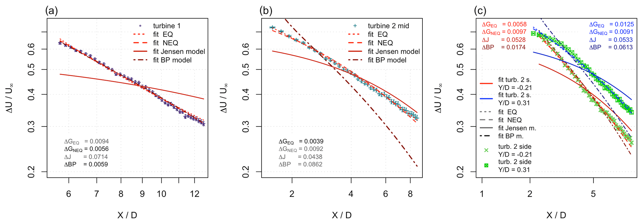
Figure 11 $\mathrm{\Delta }U/U_{\mathrm{\infty }}$ for the three different inflow conditions at the spanwise position $Y/D=-\mathrm{0.21}$: (a) turbine 1 – laminar inflow, (b) turbine 2 mid – turbulent, and (c) turbine 2 side – turbulent and intermittent. Different models are fitted to the recovery region, and the residual standard errors are presented. Note that the axes are logarithmic.

Table 3 Fit parameters and RMS errors for the different models predicting the evolution of $\mathrm{\Delta }U/U_{\mathrm{\infty }}$ for the three scenarios at the radial position $Y/D=-\mathrm{0.21}$. Note that for turbine 2 side, in addition, the parameters for the radial position $Y/D=\mathrm{0.31}$ are included.

In the case of turbine 2 side, two radial positions, $Y/D=-\mathrm{0.21}$ and $Y/D=\mathrm{0.31}$, have been used to test the wake models. It can be seen that in this complex flow, the models have greater difficulties to perform well, and the evolution of the mean velocity deficit is not captured very accurately in most cases. At $Y/D=-\mathrm{0.21}$, the bluff body wake theories perform best. For $Y/D=\mathrm{0.31}$, the error is the smallest for the EQ and NEQ models, and the velocity is predicted well at the end of the measurement range. In the cases of the Jensen model and the BP model, it can be seen that the evolution of the velocity deficit is not captured very well, which is also indicated by the RMS errors. Overall, this test illustrates that even though most of the models have been designed to fit the centerline velocity deficit, they also perform quite well in the wake core at inner radial positions. This is an interesting result because it is not easy to measure along the centerline in field measurements, and with the concept of a wake core as introduced in Neunaber et al. (2020), the application of these models is expanded.

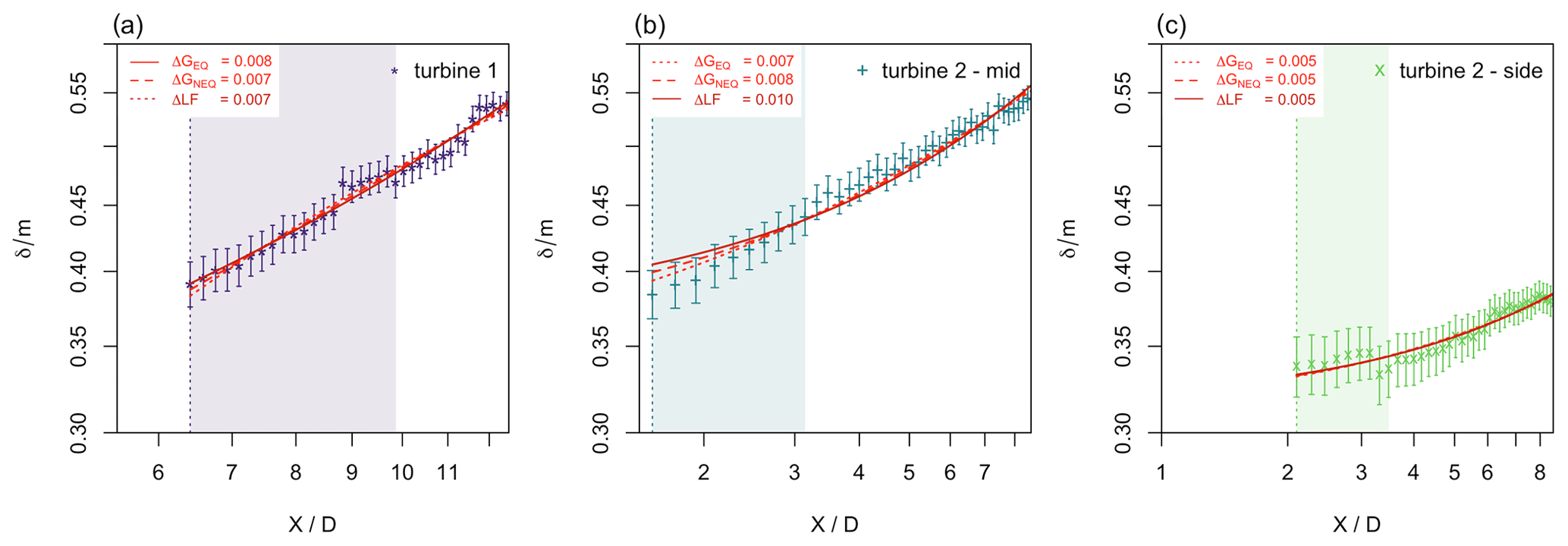
Figure 12 $\mathit{\delta }(X/D)$ for the three different inflow conditions: (a) turbine 1 – laminar inflow, (b) turbine 2 mid – turbulent, and (c) turbine 2 side – turbulent and intermittent. The EQ and NEQ models and a linear fit are applied. Note that the axes are logarithmic.

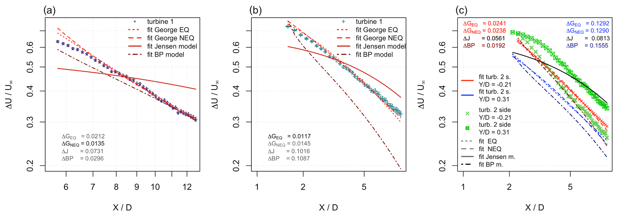
Figure 13 Modeled $\mathrm{\Delta }U/U_{\mathrm{\infty }}$ for the three different inflow conditions at the spanwise position $Y/D=-\mathrm{0.21}$: (a) turbine 1 – laminar inflow, (b) turbine 2 mid – turbulent, and (c) turbine 2 side – turbulent and intermittent. Different models are fitted to the recovery region, and the residual standard errors are presented. Note that the axes are logarithmic.

To further test the applicability of the models, in the next step, we will calculate the velocity deficit at the radial position $Y/D=-\mathrm{0.21}$ (and additionally $Y/D=\mathrm{0.31}$ in the case of turbine 2 side) from a radial correction: the BP model already has an implemented radial correction. The Jensen model is a top-hat-shaped model, and we therefore forego a radial correction. The EQ and NEQ models can be expanded by including the radial profile information from Eq. (10) to calculate the normalized velocity deficit $\mathrm{\Delta }U(Y/D)/U_{\mathrm{\infty }}$ as

$$\begin{array}{}\text{(11)}& \begin{array}{rl}{\displaystyle \frac{\mathrm{\Delta }U(Y/D)}{U_{\mathrm{\infty }}}}& =A_{\mathrm{EQ}}{U}_{\mathrm{\infty }}{\left(\left(x-x_{\mathrm{0},\mathrm{EQ}}\right)/\mathit{\theta }\right)}^{-\mathrm{2}/\mathrm{3}}\cdot a\\ & \cdot \exp \left(-b(Y/\mathit{\delta }{)}^{\mathrm{2}}-c(Y/\mathit{\delta }{)}^{\mathrm{4}}-d(Y/\mathit{\delta }{)}^{\mathrm{6}}\right)\end{array}\end{array}$$

and

$$\begin{array}{}\text{(12)}& \begin{array}{rl}{\displaystyle \frac{\mathrm{\Delta }U(Y/D)}{U_{\mathrm{\infty }}}}& =A_{\mathrm{NEQ}}{U}_{\mathrm{\infty }}{\left(\left(x-x_{\mathrm{0},\mathrm{NEQ}}\right)/\mathit{\theta }\right)}^{-\mathrm{1}}\cdot a\\ & \cdot \exp \left(-b(Y/\mathit{\delta }{)}^{\mathrm{2}}-c(Y/\mathit{\delta }{)}^{\mathrm{4}}-d(Y/\mathit{\delta }{)}^{\mathrm{6}}\right)\end{array}\end{array}$$

from the fit parameters obtained for the centerline velocity deficit and the wake profile. For this, the evolution of the wake width has to be known, and it is given by Eqs. (2) and (4). Here, we apply the equations to the evolution of $\mathit{\delta }(X/D)$, which is presented in Fig. 12 for the three scenarios, and we apply in addition a linear fit of the form $\mathit{\delta }(X/D)=\mathit{\alpha }+\mathit{\beta }\cdot (X/D)$. It can be seen that all three models perform very similarly in the measurement range and also that $\mathit{\delta }(X/D)$ increases almost linearly. From the fit parameters given in Table 4, we see that the fit coefficients B_EQ and B_NEQ of turbine 1 and turbine 2 mid are similar. As expected, the results are different for turbine 2 side, where the prediction of the wake width is not very accurate due to the complex inflow. In addition, it can be seen that the virtual origins are different from the ones obtained for the fits of the normalized velocity deficits. Therefore, while the Townsend–George theory overall holds for a wind turbine wake, there are certain details that deviate and that will need further investigation in the future.

Figure 14 $\mathrm{\Delta }U/U_{\mathrm{\infty }}$ for the three different inflow conditions at the centerline: (a) turbine 1 – laminar inflow, (b) turbine 2 mid – turbulent, and (c) turbine 2 side – turbulent and intermittent. The Jensen and the BP models are modified by including a virtual origin in the fits. Note that the axes are logarithmic.

Table 4 Fit parameters and RMS errors for the different models predicting the evolution of δ for the three scenarios.

In Fig. 13, the normalized mean centerline velocity deficit at the radial position $Y/D=-\mathrm{0.21}$ is plotted for the three scenarios, and the predicted evolutions are added for the different models. In the case of turbine 1, the EQ and NEQ models capture the evolution very well from $X/D\approx \mathrm{7}$. The best fit is achieved with the NEQ model. The BP model captures the evolution of $\mathrm{\Delta }U/U_{\mathrm{\infty }}$ in the far wake but shows deviations closer to the rotor. As expected, the Jensen model does not perform well. In the case of turbine 2 mid, the EQ and NEQ models perform similarly well and capture the evolution of $\mathrm{\Delta }U/U_{\mathrm{\infty }}$ in the measurement range, but the curves start to deviate far downstream. The BP model shows a big deviation because the centerline velocity deficit (cf. Fig. 9) was already not captured well. The Jensen model also shows strong deviations. In the case of turbine 2 side at $Y/D=-\mathrm{0.21}$, the EQ and NEQ models do underpredict the velocity deficit in the far wake, but the result is close to the measured data. The Jensen model is again strongly deviating. The BP model fits the evolution of $\mathrm{\Delta }U/U_{\mathrm{\infty }}$ best in this situation. In the case of $Y/D=\mathrm{0.31}$, none of the models perform well because they all rely on a decreasing velocity deficit towards the free flow, but in the sheared inflow situation, the velocity deficit actually increases.

As we have seen, the EQ and NEQ bluff body wake models are significantly better in predicting the normalized mean velocity deficit at $Y/D=-\mathrm{0.21}$ than the engineering wind turbine wake models. One reason is that more parameters need to be obtained from fits of the wake shape and the centerline velocity deficit. Another reason is the implied virtual origin that is common in free shear flow analysis, as it includes the transition of the wake to the final turbulent wake state. It gives these models a high flexibility to adapt to different wakes. While the concept of a virtual origin has been taken into account in the form of the initial wake width in other wake models, e.g., the Bastankhah–Porté-Agel model, a “true” virtual origin that is not limited to a value of the order of magnitude of the turbine diameter improves the flexibility. Therefore, we checked whether the Jensen and BP models can be improved by including a virtual origin, thus substituting X for X−X₀. The results are shown in Fig. 14, and the fit parameters are given in Table 5. For both models, the implementation improves the accuracy of the fits significantly so that they are now on the order of magnitude of the errors obtained for the EQ and NEQ models in some cases. Nevertheless, a similar systematic deviation can be identified in the wakes of turbine 2 mid and turbine 2 side where the centerline mean velocity deficit is overpredicted in one part of the wake and underpredicted in an other part of the wake. A clear difference in X₀ can be seen for laminar and turbulent inflow. This shows the potential for the concept of a virtual origin to include the background turbulence conditions.

Table 5 Fit parameters and RMS errors for the altered Jensen and BP models with a virtual origin (VO) predicting the evolution of $\mathrm{\Delta }U/U_{\mathrm{\infty }}$ for the three scenarios at the centerline.

6 Conclusions

In this paper we have introduced a new approach to look at the evolution of the wake of a wind turbine for the Townsend–George theory that was originally derived from bluff body wakes to predict the evolution of the mean centerline velocity deficit in a laminar incoming flow. For this, we performed wind tunnel measurements of the wake downstream of a single turbine exposed to laminar inflow and a turbine exposed to the wake of an upstream turbine and the half-wake of an upstream turbine. First, we presented a systematic study on the applicability of the Townsend–George theory to wind-turbine-generated wakes for the different incoming flows. For this, we explored the streamwise range in which all requirements are fulfilled; cf. Table 1. We found that all five requirements are (sufficiently) satisfied in the cases of turbine 1 and turbine 2 mid. The requirements are partially fulfilled in the case of turbine 2 side. Next, we studied the change of Re_λ and Re_L with downstream distance to interpret the behavior of C_ε for this flow and to draw conclusions regarding the centerline evolution of ΔU and δ (i.e., equilibrium or non-equilibrium scaling). By means of C_ε(Re_λ) being approximately constant, we found evidence for equilibrium turbulence in the investigated parts of the wake for all three scenarios. In the following step, we applied the Townsend–George theory of ΔU to estimate the velocity deficit in the three wake scenarios using the equilibrium and the non-equilibrium predictions. In addition, two engineering wind turbine wake models have been applied to the data. It was found that the Townsend–George theory does describe the wake of a wind turbine and even a second-row turbine very well. In particular, the equilibrium scaling gives good results for all three wake scenarios. Thus, the nature of the energy cascade is closer to the equilibrium scaling (i.e., the scalings consistent with the Richardson–Kolmogorov cascade) than to the non-equilibrium scaling for the different wind turbine wake flows. Especially in the more complex situation of a wake inflow, the equilibrium bluff body wake model outperforms the wind turbine wake models despite the fact that the former has been derived for the wake evolving downstream of a static bluff body exposed to uniform laminar inflow. This opens up a new perspective, as the wake of a wind turbine does behave in principal similarly in different inflow conditions. While multiple wake situations are normally solved by using wake superposition models (which are not in accordance with the Navier–Stokes equations), with our interpretation, a final turbulence state within a wind farm due to the turbulence evolution processes is plausible. A more precise description of wakes within a wind farm is of interest, as due to the cubic dependence of the power on the wind velocity, even rather small deviations in the velocity estimation can lead to large deviations in the power prediction.

To further investigate the applicability of the wake models, we also applied them to a different radial position, $Y/D=-\mathrm{0.21}$. We saw that the equilibrium bluff body wake model again outperforms the common wind turbine wake models. As the centerline is not always captured perfectly in field measurements, this result is very interesting for the application. Also, we could show that a radial correction can be used to predict the wake at $Y/D=-\mathrm{0.21}$ using the fit coefficients obtained for the centerline. In comparison to the BP model that has a built-in radial correction, the Townsend–George theory again shows better results.

The virtual origin native to the Townsend–George theory was identified as the one main advantage of the bluff body wake models. As mentioned above, this virtual origin differs from the concept of the initial wake width used in some of the engineering wake models in that it accounts for the turbulence transition (and therefore is common to several turbulence one-point quantity scalings). Therefore, we also discuss how the implementation of a virtual origin may improve the Jensen and the BP models, especially as we see that it can be used to include the inflow turbulence in the wake models.

A final result of this analysis is that C_ε does change in the wake both with respect to the radial position and with respect to the inflow condition. A consequence is that the turbulence dissipation inside a wind farm is inhomogeneous and instationary, which needs to be considered in simulations to further improve wind farm modeling. The investigation of C_ε can also be used as a tool to add information on the type of turbulence present and, thus, has the potential to refine the understanding of turbulence within a wind farm.

Overall, this work shows in a detailed manner the consistent applicability of the equilibrium turbulence bluff body wake model from turbulence theory to wind turbine wakes and thus the importance of correctly taking C_ε into account. While the Jensen model is derived from the conservation of mass and the BP model includes conservation of mass and momentum and considers the shape of the wake, we show that the additional inclusion of the turbulent nature is crucial. Nevertheless, we also see that the models fail in multi-wake scenarios where the inflow is not symmetric and where thus superposition approaches would as well fail. This and the additional dependence of the wind turbine wake on the operational state of the turbine are difficulties occurring inside find farms that need further investigation.

For the future, a more detailed investigation of C_ε inside a wind farm will be interesting in order to identify possible regions with non-equilibrium turbulence and their dependence on the inflow turbulence and the operational state of the turbine (e.g., the thrust coefficient). In addition, the possibility of expanding engineering wind turbine wake models with a virtual origin should be further explored, especially with respect to the inflow turbulence. With the extremely asymmetric example of turbine 2 side, we could show that the application of the equilibrium wake model works to a certain degree because the turbulence tends to evolve towards a symmetric wake as far as possible. This gives a good indication for new theories to model half-wake and multi-wake scenarios with asymmetric inflows where C_ε can be included.

Another open challenge will be to combine the ideas discussed here with the broader topic of wind farm wakes which are for example discussed in Platis et al. (2020) and Volker et al. (2015), who successfully “use the classical wake theory (Tennekes and Lumley, 1972) to describe the sub-grid-scale wake expansion”.

Appendix A: Estimation of turbulence quantities

To estimate the integral length scale L and the Taylor length λ, we use the one-dimensional energy spectra as proposed by Hinze (1975). As the upper boundary of the inertial sub-range, the integral length scale can be estimated calculating the limit of the energy spectrum in the frequency domain for f approaching 0 as

$$\begin{array}{}\text{(A1)}& L=\underset{f\to \mathrm{0}}{lim}\left({\displaystyle \frac{E\left(f\right)\cdot U}{\mathrm{4}u{{}^{\prime }}^{\mathrm{2}}}}\right),\end{array}$$

where u^′ is the RMS value of the fluctuating streamwise velocity U(t).

To estimate an error for the integral length scale, we use the standard deviation σ_E of the points of the spectrum that are used to estimate the limit $\underset{f\to \mathrm{0}}{lim}$ which is the “flat” part of the spectrum at low frequencies. σ_E is then expressed as a percent of the mean energy in these frequencies, ${\mathit{\sigma }}_{\mathrm{E},n}={\mathit{\sigma }}_{\mathrm{E}}/\langle E\rangle$, and $\mathrm{\Delta }L=L\cdot {\mathit{\sigma }}_{\mathrm{E},n}$.

The Taylor length is defined as

$$\begin{array}{}\text{(A2)}& \mathit{\lambda }={\left({\displaystyle \frac{u{{}^{\prime }}^{\mathrm{2}}}{\langle (\partial U^{\prime }/\partial X{)}^{\mathrm{2}}\rangle }}\right)}^{\mathrm{1}/\mathrm{2}},\end{array}$$

where $U^{\prime }=U\left(t\right)-U$ is the fluctuations of the velocity and 〈⋅〉 denotes the ensemble average. The energy spectrum in the space domain can be used to calculate $\langle (\partial U^{\prime }/\partial X{)}^{\mathrm{2}}\rangle$ as

$$\begin{array}{}\text{(A3)}& \langle {\left({\displaystyle \frac{\partial U^{\prime }\left(X\right)}{\partial X}}\right)}^{\mathrm{2}}\rangle =\underset{k_{\min }}{\overset{k_{\max }}{\int }}{k}^{\mathrm{2}}E\left(k\right)\mathrm{d}k,\end{array}$$

with the wave number k.

By means of the Taylor length λ, the RMS value of the fluctuating streamwise velocity u^′ and the kinematic viscosity ν, the Taylor Reynolds number is calculated as

$$\begin{array}{}\text{(A4)}& R{e}_{\mathit{\lambda }}={\displaystyle \frac{u^{\prime }\cdot \mathit{\lambda }}{\mathit{\nu }}}.\end{array}$$

The energy dissipation rate ε can be estimated by $\mathit{\epsilon }=\mathrm{15}\mathit{\nu }\langle (\partial U^{\prime }/\partial X{)}^{\mathrm{2}}\rangle$ (cf. Pope, 2000) under the assumptions of isotropy in small scales and the validity of Taylor's hypothesis of frozen turbulence. The derivative is calculated using Eq. (A3). Using the RMS value of the fluctuating streamwise velocity as an estimate of the turbulent kinetic energy, C_ε is calculated:

$$\begin{array}{}\text{(A5)}& C_{\mathit{\epsilon }}={\displaystyle \frac{\mathit{\epsilon }L}{u{{}^{\prime }}^{\mathrm{3}}}}={\displaystyle \frac{\mathrm{15}L}{R{e}_{\mathit{\lambda }}\mathit{\lambda }}}.\end{array}$$

The integral wake width is calculated as

$$\begin{array}{}\text{(A6)}& {\mathit{\delta }}^{\mathrm{2}}\left(X\right)={\displaystyle \frac{\mathrm{1}}{\mathrm{\Delta }U}}\underset{\mathrm{0}}{\overset{\mathrm{\infty }}{\int }}\left(U_{\mathrm{\infty }}-U\right)r\mathrm{d}r,\end{array}$$

and as the number of radial positions (six) is limited in this study, we calculate δ by applying linear interpolation between the points. We do not use Eqs. (9) or (10), as we wanted to avoid any bias that may occur due to fits deviating from the measured data. To estimate the error of δ (Δδ) we use the difference between δ calculated with linear interpolation and δ calculated from the six positions without any interpolation. This serves as an estimate of the maximum error.