the Creative Commons Attribution 4.0 License.
the Creative Commons Attribution 4.0 License.
 | 21 Oct 2022
The sensitivity of the Fitch wind farm parameterization to a three-dimensional planetary boundary layer scheme
Timothy W. Juliano
Julie K. Lundquist
David Rosencrans
Nicola Bodini
Mike Optis
Wind plant wake impacts can be estimated with a number of simulation methodologies, each with its own fidelity and sensitivity to model inputs. In turbine-free mesoscale simulations, hub-height wind speeds often significantly vary with the choice of a planetary boundary layer (PBL) scheme. However, the sensitivity of wind plant wakes to a PBL scheme has not been explored because, as of the Weather Research and Forecasting model v4.3.3, wake parameterizations were only compatible with one PBL scheme. We couple the Fitch wind farm parameterization with the new NCAR 3DPBL scheme and compare the resulting wakes to those simulated with a widely used PBL scheme. We simulate a wind plant in pseudo-steady states under idealized stable, neutral, and unstable conditions with matching hub-height wind speeds using two PBL schemes: MYNN and the NCAR 3DPBL. For these idealized scenarios, average hub-height wind speed losses within the plant differ between PBL schemes by between −0.20 and 0.22 m s−1, and correspondingly, capacity factors range between 39.5 %–53.8 %. These simulations suggest that PBL schemes represent a meaningful source of modeled wind resource uncertainty; therefore, we recommend incorporating PBL variability into future wind plant planning sensitivity studies as well as wind forecasting studies.
- Article
(6253 KB) - Full-text XML
- BibTeX
- EndNote


This work was authored in part by the National Renewable Energy Laboratory, operated by Alliance for Sustainable Energy, LLC, for the US Department of Energy (DOE) under contract no. DE-AC36-08GO28308. Funding was provided by the US Department of Energy Office of Energy Efficiency and Renewable Energy Wind Energy Technologies Office and by the National Offshore Wind Research and Development Consortium under agreement no. CRD-19-16351. The views expressed in the article do not necessarily represent the views of the DOE or the US Government. The US Government retains and the publisher, by accepting the article for publication, acknowledges that the US Government retains a nonexclusive, paid-up, irrevocable, worldwide license to publish or reproduce the published form of this work, or allow others to do so, for US Government purposes.
Despite a large demand to build offshore wind turbines in the United States, the wind resource at many potential construction sites suffers from a large degree of uncertainty. Wind resource assessments for new wind plants often involve gathering multi-year measurements of hub-height winds (Brower et al., 2012). While this approach is common for onshore sites, hub-height wind measurements are more challenging to collect offshore, and public offshore measurements are sparse within the United States. While the Bureau of Offshore Energy Management (BOEM) is considering or has already allowed commercial development in 33 renewable energy areas (BOEM, 2020), to the best of the authors' knowledge, public offshore yearlong hub-height wind speed measurements are available today in the vicinity of six sites – four due to deployments by the US DOE (accessible at https://a2e.energy.gov/data, last access: 14 October 2022) and two due to deployments by the New York State Energy Research and Development Agency (accessible at https://oswbuoysny.resourcepanorama.dnvgl.com, last access: 14 October 2022). The US is rapidly developing its offshore wind industry, recently expanding its offshore wind generation goal to 30 GW by 2030 (White House, 2021). Thus, it is critical to be able to accurately and confidently characterize wind resource in the absence of high-quality measurements for the rapidly developing offshore wind industry in the United States.
Due to limited observations, offshore wind resource assessments in the United States rely more heavily on numerical weather prediction (NWP) models. NWP-based wind resource assessments have been used to characterize wind resource in turbine-free environments (simulating winds prior to wind plant construction) as well as turbine-including environments (simulating winds after wind plant construction). While NWP models provide useful predictions of wind resource, their estimates are also accompanied by a large degree of uncertainty. As such, uncertainty quantification of offshore wind resource has been established as a key component of the US offshore wind research agenda. Shaw et al. (2019) assert that uncertainty quantification represents a critical area of offshore wind research, as “quantification and reduction of uncertainty represents a significant opportunity to reduce costs”. This sentiment was also echoed in a wind energy workshop that brought together stakeholders from industry, academia, and the US government (Haupt et al., 2020). Finally, Archer et al. (2014) underscored two major research needs for coastal and offshore wind energy research in the United States – more offshore observations and uncertainty characterization, in particular uncertainty characterization through ensembles of NWP simulations. Archer et al. (2014) also emphasized the need for research on turbine wake losses. The research in our paper directly responds to the need for ensembles of NWP simulations as well as the need to quantify wake losses.
Wind resource uncertainty in turbine-free NWP simulations stems from, in part, the large number of plausible model options that can be used to drive a simulation. Hub-height wind speeds in turbine-free NWP simulations have been shown to be significantly sensitive to a number of modeling options. Simulated wind resource has been shown to often be most sensitive to the choice of planetary boundary layer (PBL) parameterization, and PBL schemes have also been shown to be sensitive to other factors such as grid resolution (Storm and Basu, 2010; Carvalho et al., 2012; Yang et al., 2013; Carvalho et al., 2014; Draxl et al., 2014; Olsen et al., 2017; Yang et al., 2017; Fernández-González et al., 2018; Yang et al., 2019; Optis et al., 2020). PBL schemes govern turbulent fluxes (typically just vertical turbulent fluxes) and mixing within the atmospheric boundary layer. At present, 13 different PBL schemes are available within the Weather Research and Forecasting (WRF; Skamarock et al., 2021) model, and there is no single-best PBL scheme for wind resource assessment. As just one example, Draxl et al. (2014) evaluated seven PBL schemes using measurements from a meteorological mast at the Høvsøre wind energy test site. They found that the optimal PBL scheme varies with stability: at this site, MYJ (Janjić, 1994) performed best under stable conditions, ACM2 (Pleim, 2007) performed best under neutral conditions, and YSU (Hong et al., 2006) performed best under unstable conditions. Wind atlases that characterize model uncertainty often employ ensembles of simulations where model inputs, such as PBL scheme, are varied (Bodini et al., 2021a).
While the sensitivity of hub-height winds to PBL scheme has been explored in turbine-free NWP simulations, the resulting impacts on wake simulations have not been explored. To date, all published mesoscale WRF simulations with explicitly represented wind turbines have been conducted with the MYNN PBL scheme (Nakanishi and Niino, 2009; Olsen et al., 2017). Thus, while PBL schemes have been shown to be key elements for uncertainty quantification in NWP-based wind resource assessments in turbine-free environments, it is unknown if PBL schemes are similarly important in turbine-including environments. It is critical to accurately predict wake effects in order to accurately predict annual energy production. Lee and Fields (2021) summarize the large degree of uncertainty regarding the impact of wake-associated losses on annual energy production: some estimates predict average total wake losses as low as 6.1 %, whereas others have predicted losses as high as 40 %. The uncertainty in individual wake loss estimates has also been estimated to be 10 %–40 %. These losses and uncertainties incur significant financial impact on the wind industry, potentially translating to millions of US dollars of economic benefits (Lee and Fields, 2021).
While turbine-including NWP sensitivity studies have not examined the impact of PBL schemes on mesoscale wakes, they have shown that NWP-modeled wakes can be sensitive to a number of other inputs. Turbine wakes are modeled in NWP simulations with wind farm parameterizations (WFPs; for a review see Fischereit et al., 2022), such as the Fitch WFP (Fitch et al., 2012), the Explicit Wake Parametrisation (EWP; Volker et al., 2015), and the hybrid WFP (Pan and Archer, 2018). Wind resource in turbine-including simulations has been shown to be sensitive to the same model inputs that are important in turbine-free simulations, such as vertical and horizontal grid resolution, as well as the option to have the MYNN PBL scheme advect turbulent kinetic energy (TKE; Redfern et al., 2019; Tomaszewski and Lundquist, 2020; Archer et al., 2020; Siedersleben et al., 2020; Larsén and Fischereit, 2021). We note that most if not all Fitch WFP simulations with TKE advection turned on prior to Archer et al. (2020) were subject to a bug in the WRF code. As such, the results from these studies should be interpreted with caution, as it is possible that this bug may have significant impacts. Modeled wake impacts have also been shown to be sensitive to inputs specifically associated with the WFP, such as the choice of WFP and the degree of explicitly added TKE in the Fitch WFP (Fitch et al., 2012; Vanderwende et al., 2016; Siedersleben et al., 2020; Tomaszewski and Lundquist, 2020; Archer et al., 2020; Pryor et al., 2020; Shepherd et al., 2020).
In this paper, we begin to address the following question: how sensitive are modeled mesoscale wakes to the choice of PBL parameterization? Ideally, this question would be addressed by studying all 13 PBL schemes in WRF with the Fitch WFP insofar as that is possible. Here, as a first step, we compare two PBL schemes: MYNN (Nakanishi and Niino, 2009) and the recently developed NCAR 3DPBL (Kosović et al., 2020; Juliano et al., 2022). We chose the latter as it has a prognostic equation for TKE, which is important as the Fitch WFP modifies TKE fields. We make substantial modifications to the WRF code to enable the Fitch WFP to work with the NCAR 3DPBL and then conduct a set of idealized numerical experiments based on the Fitch et al. (2012) experiments. We simulate wakes in pseudo-steady idealized environments with MYNN and the NCAR 3DPBL under stable, neutral, and unstable conditions. We also examine the role of explicitly added TKE in this set of simulations. In Sect. 2, we describe the two PBL schemes, the integration of the NCAR 3DPBL with the Fitch WFP in the WRF code, and the setup of the simulations. In Sect. 3, we discuss the results of the simulations. In Sect. 4, we conclude and discuss the implications of the idealized results for real-world wind resource assessments.
2.1 MYNN and the NCAR 3DPBL
The simulations in this paper are carried out using WRF v4.3.0 with two PBL schemes: MYNN (Nakanishi and Niino, 2009; Olson et al., 2019) and the NCAR 3DPBL (Kosović et al., 2020; Juliano et al., 2022). To avoid confusion regarding nomenclature of new turbulence models, we note that the NCAR 3DPBL is different from the 3DTKE PBL scheme (Zhang et al., 2018). The WRF v4.3.0 code in this study was modified to include the NCAR 3DPBL code, which is being prepared for public release. For simplicity, we refer to the NCAR 3DPBL as simply the “3DPBL.” Both MYNN and the 3DPBL share a common origin – they are fundamentally rooted in the turbulence modeling of Mellor and Yamada (1974). Here, we use the level 2.5 MYNN and 3DPBL schemes, which both treat TKE as a prognostic variable, thus improving their utility for wind turbine modeling, because generated TKE is advected by the PBL schemes. This behavior stands in contrast to other PBL schemes, such as YSU, which does not treat TKE as a prognostic variable.
MYNN and the 3DPBL treat turbulent mixing differently. MYNN computes the vertical turbulent mixing by calculating the vertical turbulent stress divergence, and it allows the horizontal turbulent mixing to be handled externally with a Smagorinsky-type approach (Skamarock et al., 2021, Sect. 4.2 therein). In contrast, the 3DPBL directly accounts for horizontal turbulent mixing by explicitly computing the turbulent flux divergences for momentum, heat, and moisture. The 3DPBL has been implemented into WRF to allow for three different configurations following the original Mellor–Yamada developments: (i) a full 3D model, (ii) a quasi-3D model using the so-called PBL-approximation, and (iii) a 1D model using the PBL-approximation. In this analysis, we employ the second option, as the full 3D parameterization is currently too computationally expensive for yearlong wind resource assessments. When using the second option, the 3DPBL scheme handles both the vertical and horizontal turbulent mixing by computing the 3D turbulent stress divergence, in addition to the 3D turbulent flux divergence of heat and moisture. The vertical turbulent fluxes in the 3DPBL are calculated similarly to MYNN, and the horizontal turbulent fluxes are calculated analytically following Mellor and Yamada (1982) after applying the PBL approximation (i.e., neglecting the horizontal derivatives of mean quantities in addition to the vertical derivative of vertical velocity).
Aside from different approaches for horizontal mixing, the two PBL schemes also employ different master length scales and closure constants. Both schemes employ one “master” length scale, although they calculate them differently. In the simulations in this study, the 3DPBL master length scale follows Mellor and Yamada (1982), whereas the MYNN master length scale uses a different approach that simultaneously accounts for length scales that characterize buoyancy, the surface layer, and the PBL depth. The closure constants for the 3DPBL length scale come from Mellor and Yamada (1982), whereas the MYNN closure constants were updated in Nakanishi and Niino (2009).
While the values of empirical constants are different, MYNN and the quasi-3DPBL use the same formulation to parameterize turbulent momentum, heat, and moisture fluxes. For example, they parameterize the vertical flux of the u component of wind speed as
where L is the master length scale, q is , Sm is a stability function, and U is zonal velocity (Mellor and Yamada, 1982).
2.2 Integration of the Fitch WFP with the 3DPBL
To simulate wakes with the 3DPBL, we first integrated the Fitch WFP with the 3DPBL inside the WRF code. The Fitch WFP modifies flow in two key manners (Fitch et al., 2012; Archer et al., 2020): by slowing winds
and by adding TKE
In the above equations, k is the vertical level that intersects the rotor, Ak is the area of the rotor on this vertical level, CT is the thrust coefficient, Uk is the wind speed, uk is the zonal wind, vk is the meridional wind, and zk is the height. The turbulence coefficient CTKE is calculated as the difference between the thrust coefficient CT and the power coefficient CP. The thrust and power coefficients are functions of wind speed that are unique to a particular wind turbine, and their values are specified in the input file wind-turbine.tbl. The coefficient α was introduced by Archer et al. (2020) to empirically modify the amount of explicit TKE addition, and, in this study, we set it to either 0 or 1.
The major challenge in integrating the Fitch WFP and the 3DPBL is that the 3DPBL code is housed in the dynamics (dyn_em/) part of the code, as opposed to the physics (phys/) part of the code, where most other PBL schemes reside. As such, the code base was substantially modified to account for the user-selected PBL scheme. A call to the Fitch WFP's dragforce subroutine was added to the end of dyn_em/module_first_rk_step_part2.F. When called for the 3DPBL, the velocity tendencies and TKE tendencies are additionally scaled by the column mass in order to match the identical scaling that happens to the phys/-calculated tendencies earlier within dyn_em/module_first_rk_step_part2.F. Additionally, whereas the Fitch WFP code modifies the MYNN TKE field directly (including a time step factor of ∂t), the new code modifies the 3DPBL TKE tendency field (omitting a factor of ∂t and letting the rest of the code carry out the time integration).
2.3 Configuration of simulations
We carry out a series of idealized simulations to study the effect of the PBL scheme on simulated wake dynamics in a simple offshore environment. All simulation inputs can be found on Zenodo (https://doi.org/10.5281/zenodo.5565399). We use the neutral idealized simulations of Fitch et al. (2012) as inspiration for our simulations, but we make a number of modifications. All simulations use two domains, each 202×202 grid points in the horizontal. MYNN is always used in the outer domain, whereas the inner domain is either MYNN or the 3DPBL. The outer domain uses a horizontal grid spacing of 3 km and a time step of 9 s, whereas the inner domain uses a horizontal grid spacing of 1 km and a time step of 3 s. The vertical grid uses 81 cells, up to a height of 20 km. Vertical grid stretching is employed to provide finer resolution near the surface, thereby allowing 28 vertical levels below a height of 300 m, following the recommendation of Tomaszewski and Lundquist (2020) for nominally 10 m of resolution near the surface. All simulations have a roughness length of 0.0001 m, which is characteristic of offshore environments (Stull, 1988).
In order to eventually simplify wake comparisons, we force all turbine-free simulations in such a manner that average hub-height wind speeds are roughly equal (∼9.35 m s−1) after they are spun up (Table 1). In principle, we could have matched the geostrophic winds instead of the hub-height winds in the idealized simulations, but the resulting different hub-height wind speeds would have made it more difficult to isolate the different turbulent recovery effect that comes with using the 3DPBL instead of MYNN.
Table 1A summary of boundary conditions and spinup times for the turbine-free idealized simulations.
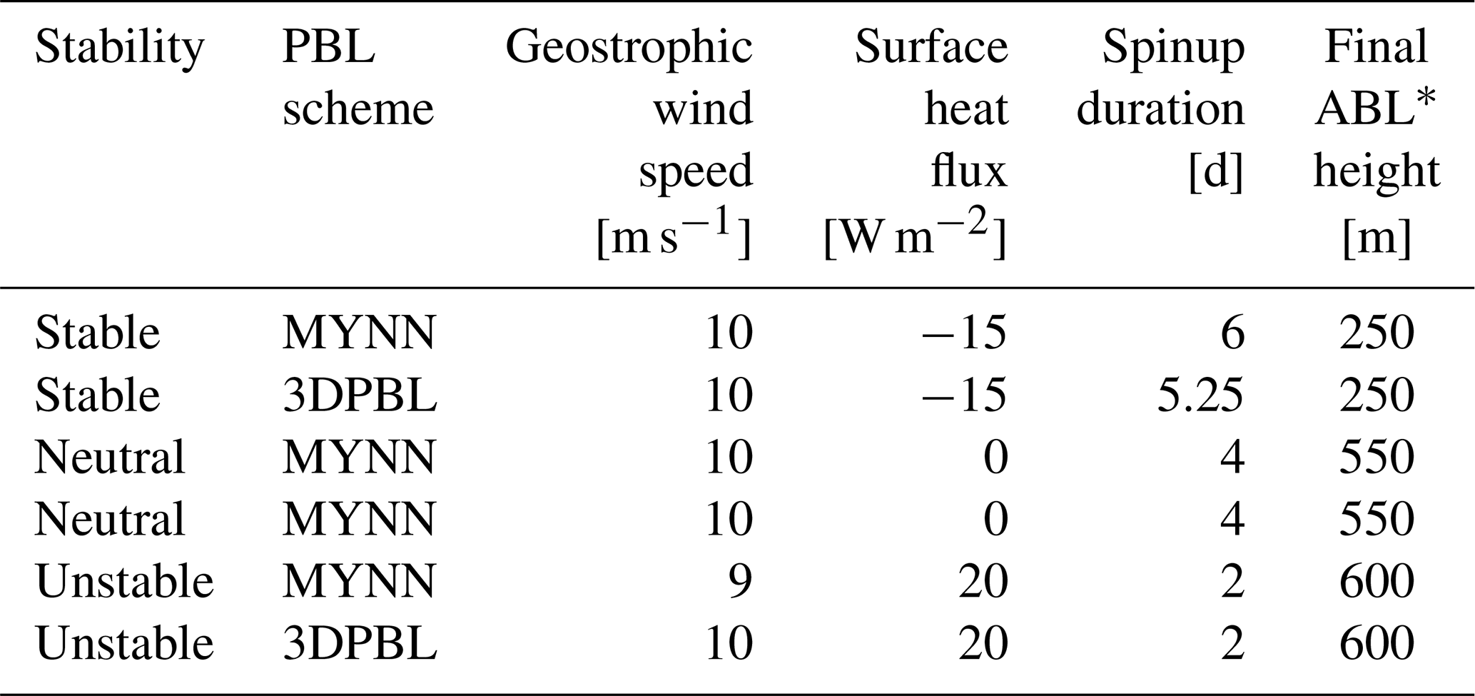
* ABL means atmospheric boundary layer.
Simulations for each stability case are initialized with a neutral temperature profile of 285 K within the boundary layer up to 500 m. The boundary layer is capped with a two-layer inversion: a strong inversion (5 K warming between 500 and 600 m) and a weaker inversion (3 K km−1 lapse rate above 600 m). Depending on the case, each simulation was forced with either 9 or 10 m s−1 geostrophic winds. Stable simulations are additionally forced with −15 W m−2 surface cooling, and unstable simulations are forced with 20 W m−2 surface heating. These sensible heat flux values were chosen based on typical simulated conditions at a planned offshore plant in the US mid-Atlantic (Rybchuk, 2022) and are smaller than typical values over land. After spinup, the boundary layer height as determined through the turbine-free temperature profile (Fig. 2) is approximately 250 m in the stable simulations, 550 m in the neutral simulations, and 600 m in the unstable simulations.
After spinning up turbine-free simulations, we run three cases of simulations for each of the stabilities and each of the PBL schemes for 24 h. The first case is simply a continuation of the turbine-free simulations and is referred to as the no-wind-farm (NWF) case. The second case (100TKE) starts after the respective NWF simulation has spun up and shares its boundary conditions, but it includes a 10×10 grid of turbines based on the 12 MW International Energy Agency (IEA; Beiter et al., 2020) reference offshore wind turbines placed in the center of the inner domain. The turbine hub height is 138 m, and the rotor diameter is 215 m. Cut-in speed is 3 m s−1, rated speed is 10.9 m s−1, and cut-out speed is 30 m s−1. Turbines are placed 2 km apart, which is close to 1-nautical-mile spacing. In this case, 100 % of explicit TKE is generated by the Fitch WFP (α=1). In the third case (0TKE), we explore the sensitivity to explicitly added TKE by duplicating the setup of the second case, but turning off explicit TKE generation (α=0).
3.1 Turbine-free conditions
We spin up the idealized turbine-free simulations so that hub-height wind speeds achieve a pseudo-steady state as well as a value of approximately 9.35 m s−1 (Fig. 1). As was observed in Fitch et al. (2012), inertial oscillations occur in neutral conditions, but they sufficiently dampen out in our simulations after 4 d. Unstable simulations initially show hub-height wind speed behavior that is similar to the neutral simulations. However, surface warming initiates thermal turbulence during the first day of spinup, and after 24 h of spinup, the hub-height wind speed behavior becomes stationary. Stable simulations show an initial hub-height wind speed spike due to the development of a low-level jet (LLJ; Fig. 2), but the wind speeds linearly decay over time as the nose of the LLJ moves upward. The stable MYNN and 3DPBL simulations achieve the target wind speed after 6 and 5.25 d, respectively.
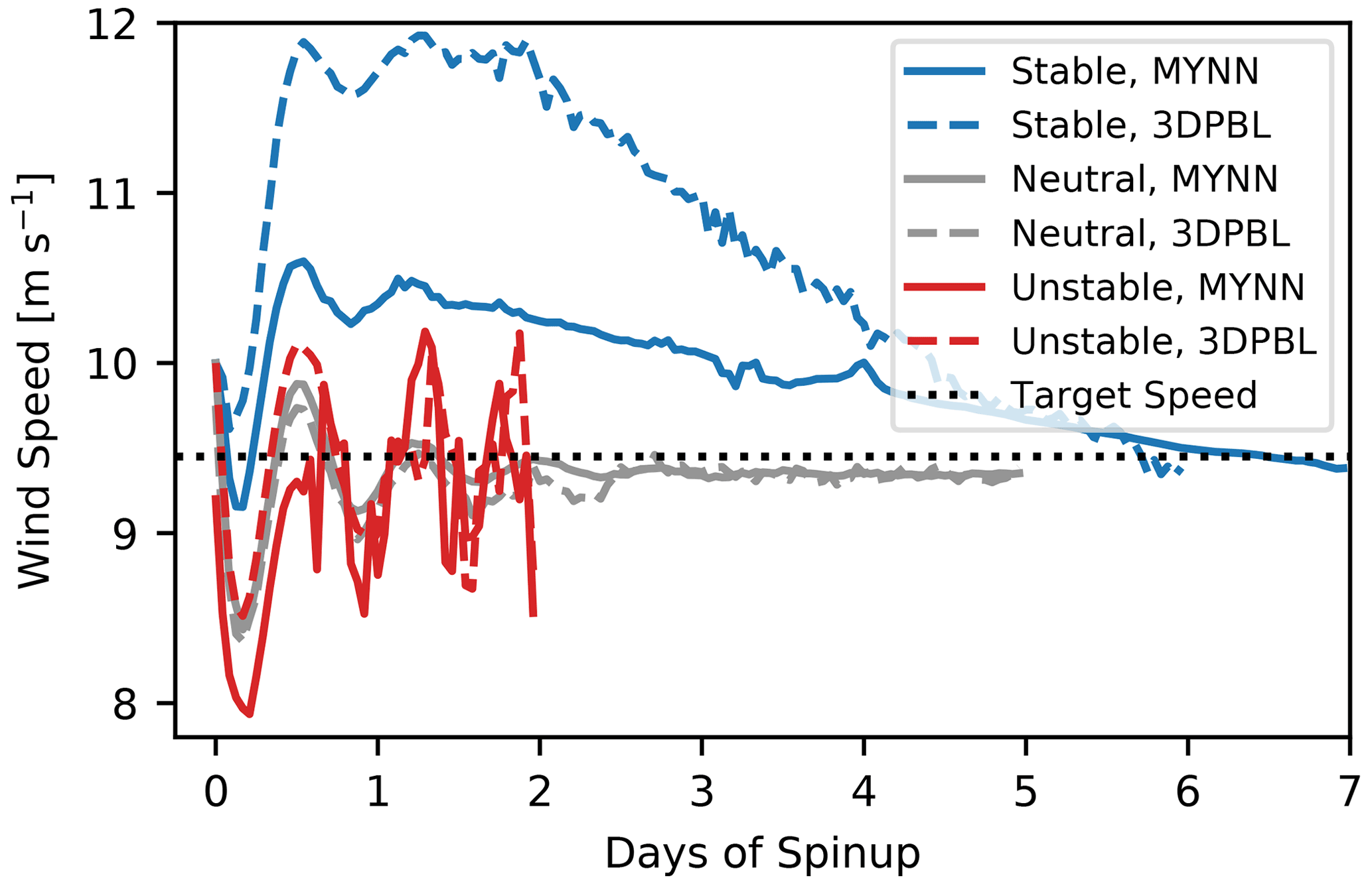
Figure 1Hub-height wind speed at the center of each domain during spinup in the idealized turbine-free simulations. The last 24 h of each simulation is taken as the performance period for the NWF simulations.
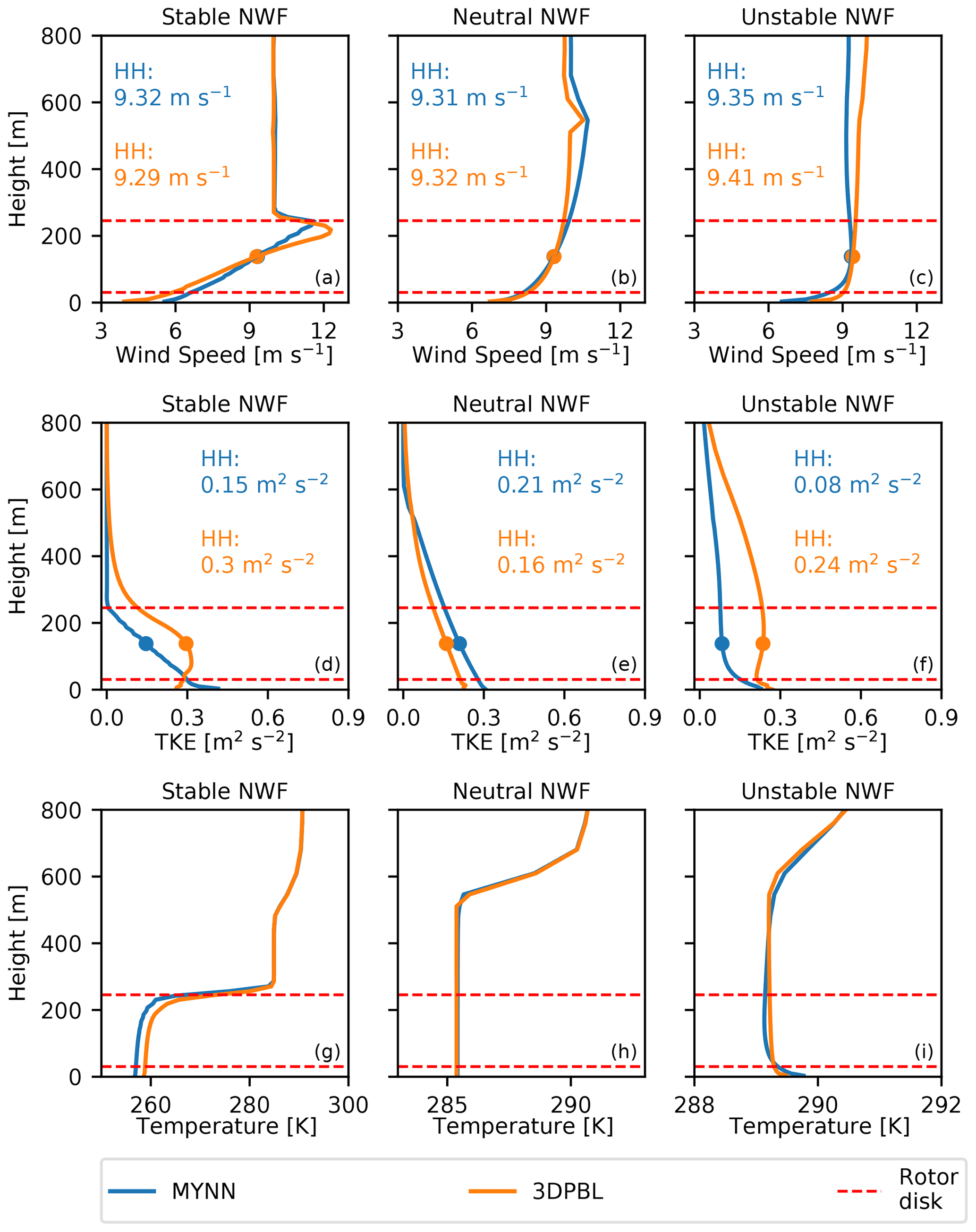
Figure 2Averaged wind speed profiles (a–c), TKE profiles (d–f), and temperature profiles (g–i) in different stabilities for the idealized NWF runs. Profiles have been horizontally averaged over the extent of the plant and time-averaged over the 24 h performance period. Hub-height values of wind speed and TKE for each PBL scheme are noted.
Having discussed the initial transient phase of the idealized simulations, it is also necessary to characterize the baseline wind speeds and TKE values in the turbine-free simulations (NWF) before analyzing turbine impacts (Fig. 2). The differences and similarities in the wind and TKE profiles of the NWF simulations will dictate the comparison of the wake effects between the PBL schemes in turbine-including simulations. In general, MYNN and the 3DPBL will predict differing wake effects because of two primary factors: different predictions of turbine-free wind speed profiles and differing wake recovery behavior, which is linked to parameterizations of turbulent fluxes (Gupta and Baidya Roy, 2021). Due to the experimental configuration of our idealized simulations, the plant inflow wind speeds are similar, and thus we expect the largest wake differences to arise from differing turbulent recovery behavior.
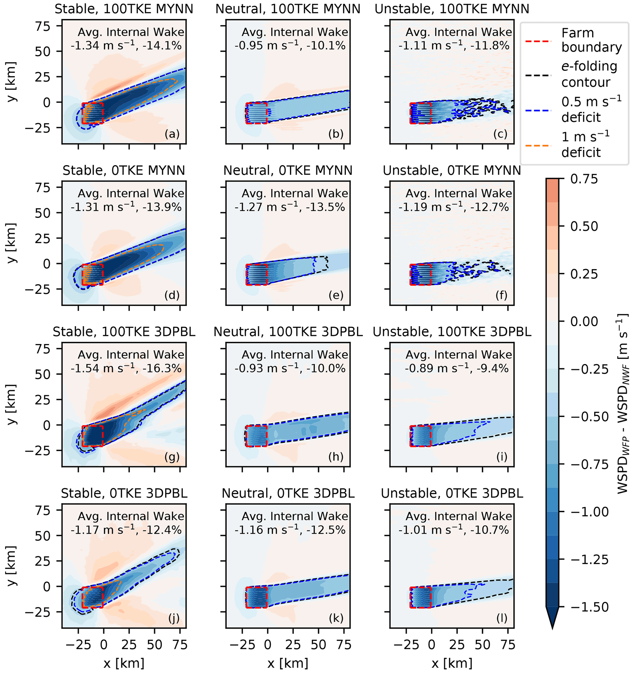
Figure 3Hub-height wind speed deficits in varying stabilities (left–right) and PBL configurations (up–down). Average hub-height wind speed deficits inside the plant are noted – in both absolute magnitude and as a percentage relative to the NWF winds. The 1 m s−1 deficit contour is highlighted only for the stable simulations, as it obscures internal wakes for other stabilities. Wakes are rotated from the u-geostrophic wind due to the combination of friction and the Coriolis force.
During the performance phase, all simulations have similar average hub-height wind speeds: between 9.3 and 9.4 m s−1. The wind speed profiles for both PBL schemes match expected canonical behavior for each stability (Stull, 1988). Across the rotor disk, the neutral and unstable wind speed profiles have similar values for both MYNN and the 3DPBL. However in the stable simulations, wind speed profiles slightly differ between the two PBL schemes. The nose of the MYNN low-level jet achieves a wind speed of 11.6 m s−1 and sits at the top of the rotor disk. In contrast, the nose of the 3DPBL LLJ achieves a wind speed of 12.3 m s−1 and sits about 40 m below the top of the rotor disk. Thus, we later see that the height of maximum wind speed deficits differs between the two simulations (Fig. 4).
While MYNN and the 3DPBL produce near-identical TKE profiles in neutral conditions, their TKE profiles differ in stable and unstable conditions. In stable conditions, the MYNN TKE profile linearly decays when moving from the surface to the capping inversion, whereas the 3DPBL profile shows an irregular shape that somewhat resembles the wind speed profile of an LLJ. In unstable conditions, the TKE profiles are relatively constant over the height of the rotor disk, but the 3DPBL TKE values are 2–3 times larger than the MYNN values. Contrary to what might be expected, we note that hub-height values of TKE are weaker in the unstable MYNN simulations than in the neutral MYNN simulations. We hypothesize that these low TKE values occur due to the very weak heat fluxes.
3.2 Hub-height wind speed deficits
Wakes within the extent of the plant are sensitive to the choice of PBL scheme, presence of explicit TKE generation, and stability (Fig. 3). We quantify wind speed deficits inside the plant by finding the daylong time-averaged hub-height wind speeds within the plant in the turbine-including simulations (“WFP”, which is a generic stand-in for “100TKE” or “0TKE”) relative to hub-height winds in the turbine-free simulations (“NWF”). We also calculate the percentage of wind speed loss with reference to the NWF winds inside the plant. Before discussing the impact of PBL scheme, we reiterate that previous work at offshore wind farms demonstrates that stability impacts waking (Hansen et al., 2012), and our idealized wakes follow expected trends: stable wakes are strongest (1.17–1.54 m s−1, 12.4 %–16.3 %), followed by neutral wakes (0.93–1.27 m s−1, 10.0 %–13.5 %), followed by unstable wakes (0.89–1.19 m s−1, 9.4 %–12.7 %).
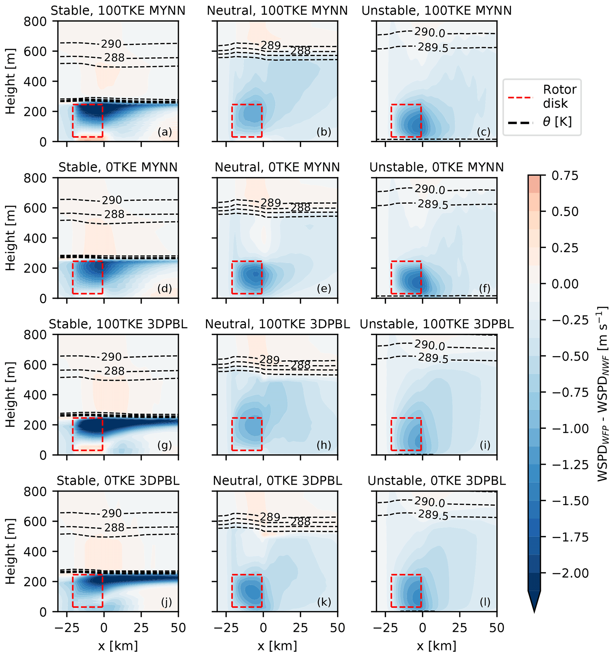
Figure 4Side view of horizontally averaged wind speed deficits in varying stability conditions (left–right) and PBL configurations (up–down). Horizontal averaging was taken between the northernmost and southernmost turbines. The height of the ABL is conveyed with θ contours.
Average wind speed deficits inside the plant can vary quite substantially between MYNN and the 3DPBL. Across all simulations, MYNN predicts internal waking that differs from the 3DPBL by between −0.20 m s−1, or −2.2 percentage points (pp; in the stable 100TKE simulations), to +0.22 m s−1, or +2.4 pp (in the unstable 100TKE simulations). This large spread induces significantly different predictions of power production (Sect. 3.6).
While these simulations show that wakes within the plant can substantially differ, they do not reveal any obvious patterns of how they will differ across conditions. At times, the MYNN simulations produce stronger wakes internally than the 3DPBL, whereas MYNN wakes are weaker at other times. Sometimes, turning explicit TKE addition off decreases the internal wake magnitude (e.g., stable conditions), whereas other times it increases internal wake strength (e.g., neutral and unstable conditions). Sometimes MYNN internal wake strength changes more substantially when explicit TKE addition is turned off (e.g., neutral and unstable conditions), whereas 3DPBL internal wake strength changes more substantially at other times (e.g., stable conditions). Thus, this variability within the idealized runs suggests that real-world case studies should be tailored to a specific region and turbine configuration.
In addition to characterizing wakes within the extent of the plant, we analyze wakes outside the plant. There is no singular standard approach that is used to characterize wakes external to a plant (Fischereit et al., 2022), so we adopt three approaches: by identifying the contours of the 1 m s−1 deficit, by identifying the contours of the 0.5 m s−1 deficit, and by identifying the e-folding contour. We calculate the e-folding contour as times the average internal wake strength, or about 36 % (Fitch et al., 2012), and as such, this uses a relative metric, whereas the other contours use an absolute metric. We employ the 1 m s−1 contour to highlight regions of strong external waking and the 0.5 m s−1 contour to emphasize moderate external waking. We only include the 1 m s−1 deficit contour in the stable simulations, as this contour obscures internal wakes in the neutral and unstable simulations. We note that choosing one definition versus the other can lead to definitions of wake lengths that differ by tens of kilometers.
Wake behavior outside the plant varies just as much as it did inside the plant (Fig. 3). The most severe waking, demarcated by the 1 m s−1 deficit contour, varies with stability as expected from previous work, with the strongest wakes in stable conditions. The 1 m s−1 contours extend the farthest in stable conditions, whereas they travel at most about 10 km downwind in neutral and unstable conditions. We note that MYNN predicts wakes that are tens of kilometers longer than the 3DPBL does in stable conditions. The addition of explicit TKE consistently increases the wake length, regardless of what metric is used to define the boundary of the wake. This increase is seen most clearly in the neutral MYNN simulations (Fig. 3b and e), where wake length grows by dozens of kilometers. All stable and all unstable simulations show a growth in wake lengths, roughly on the scale of about 10 km. We also note that neither MYNN nor the 3DPBL show consistently longer wake lengths across all stabilities. Stability impacts on moderate-intensity wakes (either the 0.5 m s−1 contour or the e-folding contour) are more varied. For example, the e-folding contour is smaller in the stable 3DPBL simulations than in the neutral 3DPBL or unstable 3DPBL simulations.
We briefly digress from the discussion on wakes to discuss two effects that are secondary to the primary analysis of this study: upwind blockage and flow acceleration. Upwind blockage (Schneemann et al., 2021; Sanchez Gomez et al., 2021) occurs in some of the idealized simulations. Blockage is strongest in the stable conditions, where 0.5 m s−1 deficits extend 5–10 km upwind of the plant. Under neutral conditions, blockage of up to 0.25 m s−1 extends 3–5 km upwind of the plant. Blockage does not appear in the unstable simulations. In general, blockage here is a function of stability but not PBL scheme or TKE addition. Tangential flow accelerations, similar to the speed-ups seen by Nygaard and Hansen (2016), can be observed adjacent to the wakes. The hub-height wind acceleration neighboring the wakes is also a function of stability (strongest in stable conditions, weakest in unstable conditions), but it also varies with TKE addition (stronger acceleration when TKE addition is turned on).
3.3 Vertical structure of wind speed deficits
While hub-height winds are particularly important to quantify, it is also helpful to characterize wakes over the vertical extent of the rotor disk. We calculate the wind speed deficit averaged across the y extent (predominantly crosswind) of the plant for each simulation (Fig. 4). Just as the top-down view (Fig. 3) of wind speed deficits suggested, the stable simulations produce the strongest wind speed deficit profiles. Blockage is also visible upwind of the plant in stable conditions. In contrast, the neutral and unstable simulations produce wind speed deficits that are relatively similar to one another. The stronger stable wind speed deficits occur, in part, because of the shallow capping inversion that sits just above the top of the rotor disk. The wakes in the neutral and unstable simulations are able to mix with stronger ambient winds above the plant, thereby eroding the wake, whereas this behavior is not possible in the stable simulations.
The side view of wind speed deficits shows that vertical mixing of wind speed deficits increases when explicit TKE generation is turned on. This behavior consistently occurs across all simulations. The wind speed deficits above the wind plants are stronger in the neutral 100TKE simulations and in the unstable 100TKE simulations than in their counterparts with 0TKE. As a result, the neutral and unstable 0TKE simulations have stronger maximum wind speed deficits within the rotor disk than their 100TKE counterparts. For example, the neutral 100TKE MYNN simulation shows a maximum wind speed deficit of 1.125 m s−1 within the rotor disk, whereas the neutral 0TKE MYNN has a maximum deficit of 1.625 m s−1. While the shallow capping inversion in the stable simulations obscures the effects of explicit TKE addition above the plant, the TKE effects can be seen below the plant. When explicit TKE addition is turned on in the stable simulations, flow acceleration occurs below the rotor disk, but this acceleration does not occur when TKE addition is turned off. We note that acceleration under the rotor disk was observed in Bodini et al. (2021b) but not in Archer et al. (2019). Correlating with the presence of flow acceleration below the rotor disk, the stable 100TKE simulations show stronger wind speed deficits within the rotor disk than the stable 0TKE simulations.
Finally, the side view of wind speed deficits also shows that the choice of PBL scheme can be important. The most pronounced differences between PBL schemes occur in stable conditions. For example, the wind speed deficit in the 0TKE 3DPBL simulation stays stronger than 2 m s−1 for 50 km downwind of the plant, whereas the wake recovers more quickly in the 0TKE MYNN simulation.
3.4 Difference in momentum tendencies
In large part, the two PBL schemes produce different wind speed deficits in their wakes because the schemes parameterize turbulent fluxes differently, as we visualize here. The u and v components of wind speed are modified by mechanisms such as advection of the mean wind, the Coriolis force, and the divergence of the turbulent momentum fluxes (Stull, 1988, Eq. 3.4.3c therein). We expect all these terms, aside from the divergence of turbulent momentum fluxes, to be similar for both MYNN and the 3DPBL, as the NWF wind speeds are similar, but two PBL schemes parameterize momentum fluxes uniquely. We calculate the u tendency due to the turbulent flux divergence as the vertical derivative of , neglecting the horizontal components of flux divergence because they are significantly smaller in the 3DPBL than , and they are not computed in the MYNN parameterization. We also omit visualizations of v tendency because they are substantially smaller than the u tendency in these idealized simulations forced with a u-geostrophic wind. We investigate the relationship of wind speeds and turbulent fluxes between the two PBL schemes in the stable 100TKE simulations by comparing two fields in the wakes – the wind speed deficits and the turbulent flux divergence u-tendency “deficits” (Fig. 5). The u-tendency deficits are defined as tendencies in the turbine-free simulations subtracted from tendencies in the turbine-including simulations.
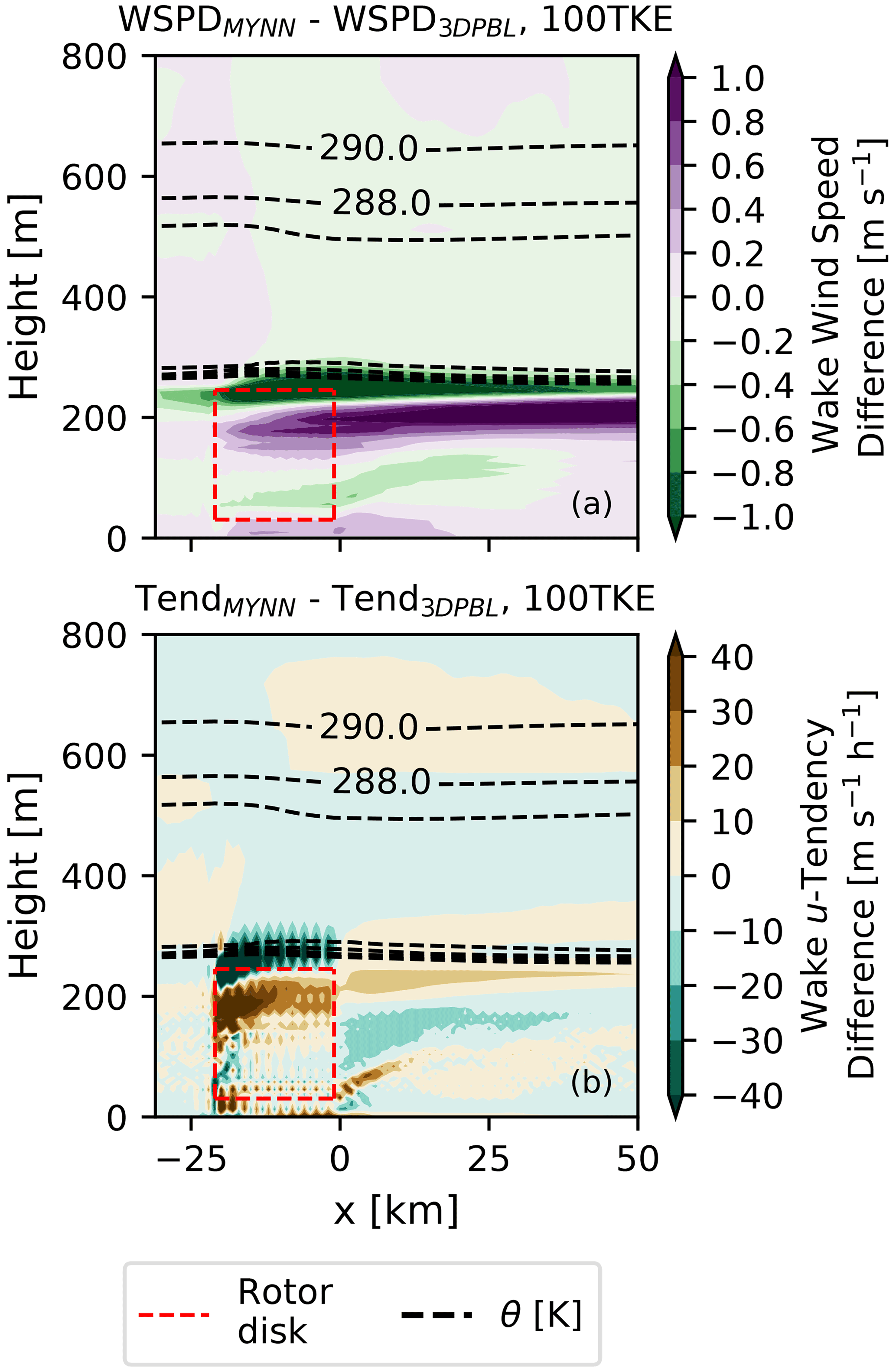
Figure 5(a) Side view of the difference in wind speed deficits in the stable 100TKE simulations. For example, (a) was calculated as the difference between the results in Fig. 4a–g. (b) The u-tendency deficits in the 100TKE simulations are calculated using a similar procedure involving tendencies. Potential temperature θ values that have been averaged over the y extent of the plant are taken from the MYNN simulations.
The differences in tendency deficits between the two PBL schemes drive the differences in the wind speed wakes. As winds advect primarily along the x direction, wind speed magnitudes are modified by the tendency. For example, the u tendency is more negative for MYNN above the rotor disk. Correspondingly, the MYNN wind speed deficits in this region as well as downwind of this region are more negative. The same pattern of behavior occurs in the upper half of the rotor disk, where the u tendency for the 3DPBL is more negative, and therefore the 3DPBL wind speed deficits are more negative. Thus, the modeled wind speed deficits in the wake of a plant depend on how the PBL scheme parameterizes turbulent momentum fluxes.
3.5 Total TKE
Just as wind speed deficits are sensitive to the choice of PBL scheme, TKE associated with the wind plant also varies as a function of PBL scheme, stability, and explicit TKE generation (Fig. 6). The WFP induces changes in TKE, and the changes are primarily constrained within the horizontal extent of the plant and tend to not advect far downwind. In contrast, the real onshore WRF WFP simulations of Mangara et al. (2019) saw substantial TKE changes 20–30 km downwind. The 100TKE simulations produce substantially more TKE than the 0TKE simulations, as would be expected. The 100TKE 3DPBL simulations also consistently predict stronger levels of additional TKE than their MYNN counterparts. For example, the maximum added TKE in the 100TKE stable simulations was 1.375 m2 s−2 for the 3DPBL and 0.750 m2 s−2 for MYNN.
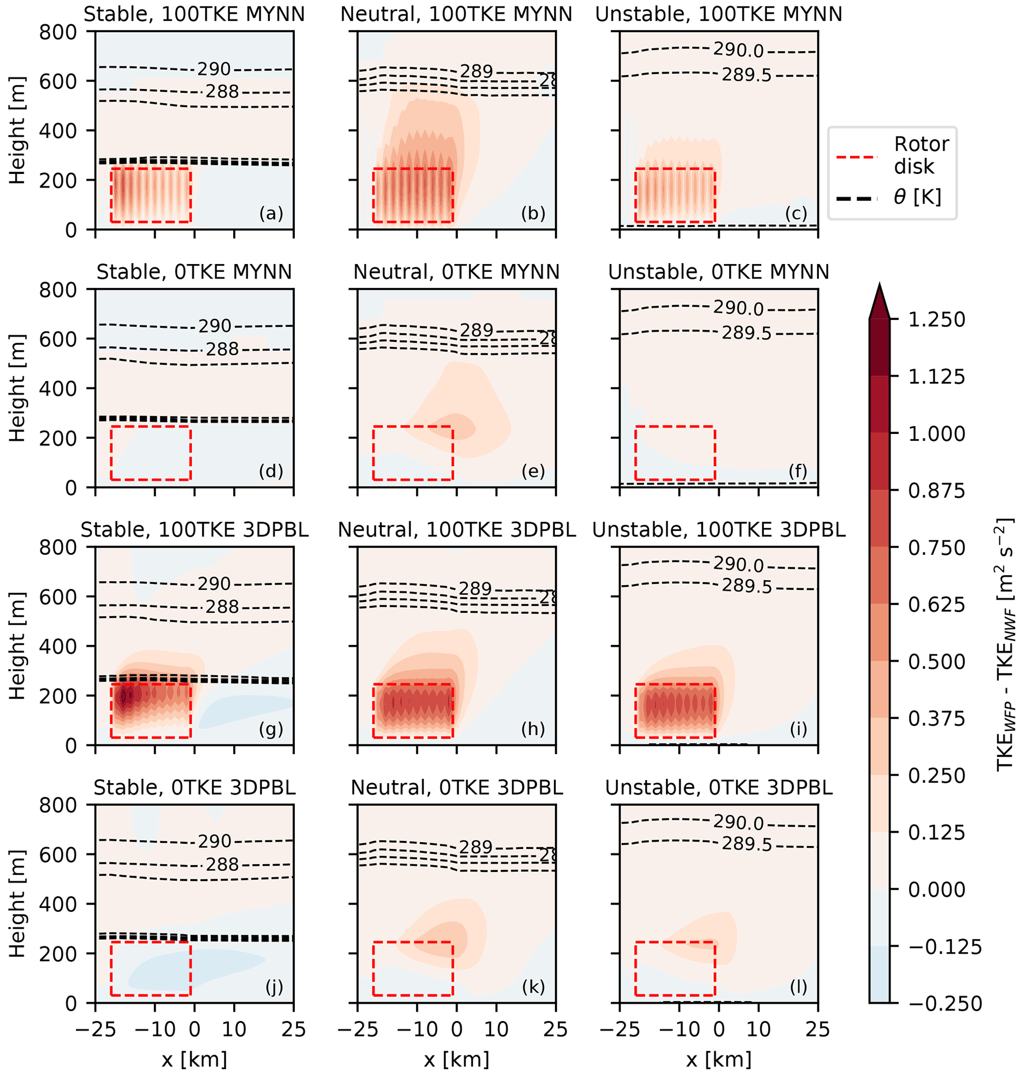
Figure 6Same as Fig. 4, but for TKE in varying stabilities (left–right) and PBL configurations (up–down). The height of the ABL is visualized in the stable and neutral simulations with θ contours.
The behavior of the 0TKE simulations was more varied. In neutral conditions, both the 0TKE MYNN and 0TKE 3DPBL simulations create a moderate amount of shear-generated TKE at the top of the rotor disk. However in unstable conditions, the 0TKE 3DPBL simulation shows shear-generated TKE, whereas the 0TKE MYNN simulation does not. In stable conditions, the 0TKE simulations lack shear-generated TKE at the top of the rotor disk due to the low capping inversion. However, the stable 0TKE 3DPBL turbine-including simulation actually has less TKE than the turbine-free simulation. The LLJ in the turbine-free simulation exhibits strong wind speed shear, and the presence of the wind farm reduces that shear, leading to this behavior.
3.6 Power
Power production and power losses due to internal waking change with PBL scheme (Fig. 7). We calculate the capacity factor for each turbine, the average capacity factor of the plant, and the average power deficit due to internal wakes with reference to the NWF hub-height wind speed. Capacity factor is defined as the ratio of actual power output relative to the maximum possible power output. Across all simulations, the average capacity factor for the plant ranged between 39.5 % and 53.8 %. Capacity factor losses due to internal wakes ranged between 16.7 and 31.6 pp.
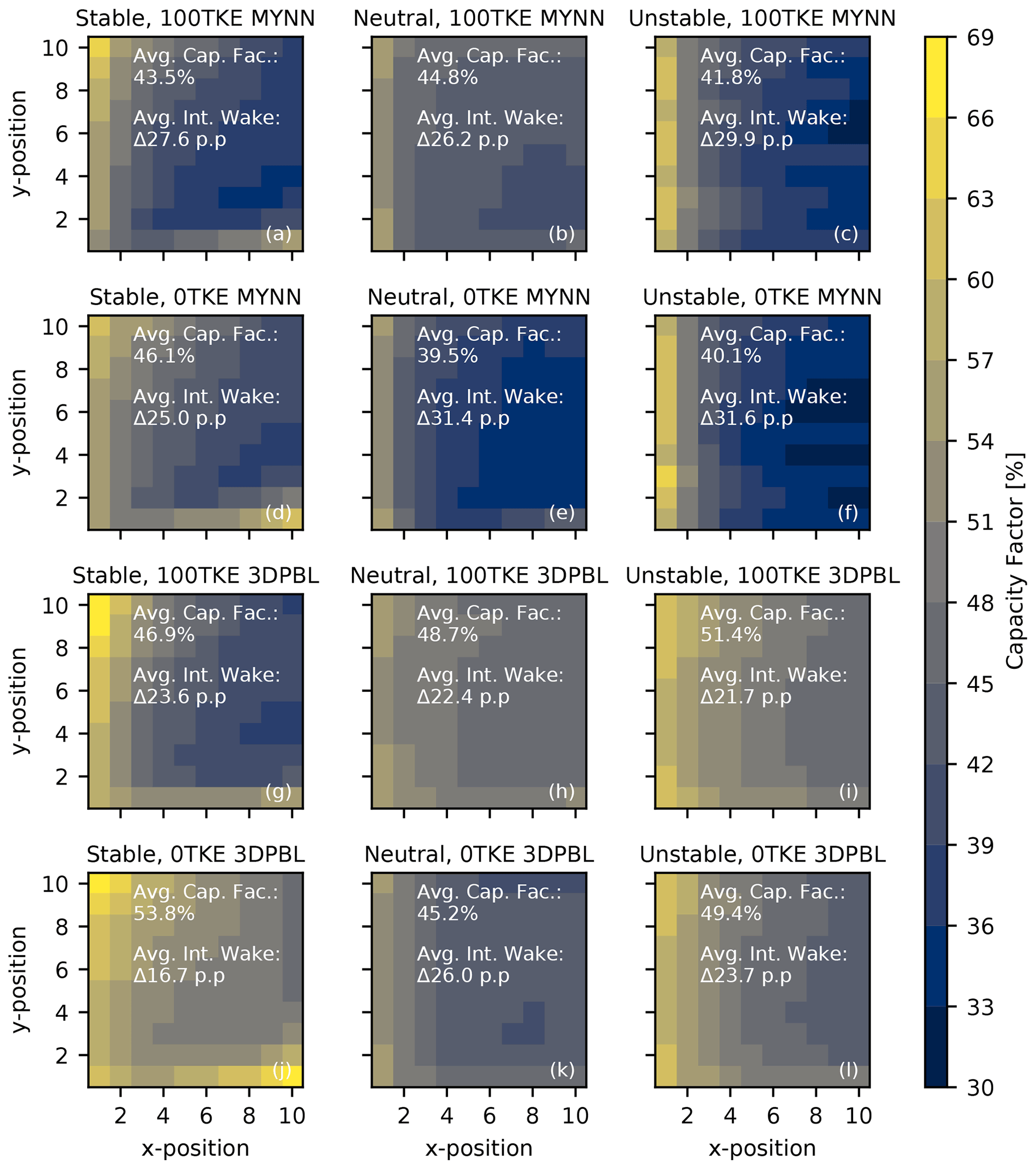
Figure 7Heat maps of capacity factor for each turbine, based on the turbine's position in the plant. The average capacity factor and internal wake strength are noted for each simulation.
Power production in the idealized simulation varies with the simulation parameters. As discussed earlier (Sect. 3.2), when explicit TKE addition is turned off, hub-height wind speed deficits can either increase or decrease. Accordingly, turning off explicit TKE generation can either grow or shrink the capacity factor. Turning off explicit TKE generation changes internal wake losses to the capacity factor by between −6.9 pp (in the stable 3DPBL) and 5.2 pp (in neutral MYNN). Changing from one PBL scheme to another results in wake loss shifts of a similar magnitude – switching from MYNN to the 3DPBL changes internal wake losses by between −3.4 pp (in stable 100TKE simulations) and −9.6 pp (in unstable 100TKE simulations). Thus, these simulations emphasize the critical role of PBL scheme on power production.
In the end, these power calculations emphasize that the behavior of modeled power losses is complicated, even in a simple idealized environment. We stress that these idealized simulations have been carried out for one set of hub-height winds in one part of the power curve under pseudo-steady conditions. To better predict the cumulative non-linear interactions of the effects of these parameters on losses at a real-world location, it is critical to run real simulations.
In this analysis, we studied the sensitivity of NWP-modeled mesoscale wakes to two PBL schemes: the widely used MYNN and the recently introduced NCAR 3DPBL. While prior studies have shown that NWP-modeled wind resource in turbine-free simulations can significantly vary with PBL scheme, the same sensitivity has not yet been studied in simulations with explicitly resolved turbines. We integrated the NCAR 3DPBL with the Fitch wind farm parameterization and then examined modeled wake sensitivity through a series of simulations. We simulated pseudo-steady idealized stable, neutral, and unstable environments with hub-height wind speeds of approximately 9.35 m s−1. In this context, we also examined wake sensitivity to the amount of explicitly added TKE from the Fitch wind farm parameterization.
We summarize key findings from this analysis.
-
In the idealized simulations, both capacity factor and wake losses were substantially impacted by PBL scheme, the presence or omission of explicit TKE addition, and the stability. Average capacity factors ranged between 39.5 %–53.8 %, and wakes reduced the average capacity factors by 16.7–31.6 percentage points.
-
Similarly, wind speed deficits were significantly impacted by these factors in the idealized simulations. MYNN predicted average wind speed deficits within the extent of the plant that differed from those in the 3DPBL by between −0.20 and 0.22 m s−1 (or between −2.2 and 2.4 percentage points for relative wake magnitude). Additionally, MYNN predicted strong external wakes that traveled dozens of kilometers longer than the 3DPBL in stable conditions.
-
While the magnitude of wind speed deficits typically varied with PBL scheme, an obvious pattern did not emerge. At times, MYNN predicted stronger deficits, whereas sometimes the 3DPBL had stronger deficits. In contrast, wakes consistently grew longer when explicit TKE addition was turned on.
Through our study, we begin to address the question of how sensitive modeled mesoscale wakes are to the choice of PBL parameterization. We find that, indeed, modeled mesoscale wakes can be significantly sensitive to the choice of PBL scheme in idealized simulations. This suggests that real mesoscale simulations of planned wind plants could also be significantly sensitive to the choice of PBL scheme. Indeed, preliminary offshore simulations in the US mid-Atlantic show that MYNN and the 3DPBL can predict month-long power production that differs by as much as 7.8 % (Rybchuk, 2022). Due to the model sensitivity discussed throughout this paper, we recommend that future wind energy planning studies that examine mesoscale model sensitivity consider varying the PBL scheme, along with other model inputs that have been established in the literature, such as grid resolution, magnitude of explicit TKE addition, and the choice of wind farm parameterization (Fischereit et al., 2022). By better characterizing the uncertainty associated with NWP-modeled wind resource, wind plant developers will be able to take on less risk when developing future wind plants.
Name lists for all simulations, time-averaged idealized WRF data, WRF code modifications, and analysis notebooks to reproduce all figures can be found on Zenodo (https://doi.org/10.5281/zenodo.5565399; Rybchuk et al., 2021).
All co-authors played an important role in this paper. Following the CRediT taxonomy, each co-author contributed to the following: AR contributed to the methodology, investigation, data curation, writing of the original draft, and writing of edits. TWJ contributed to methodology, software, and writing of edits. JKL contributed to the project conception, funding acquisition, project administration, supervision, and writing of edits. DR contributed to the methodology. NB contributed to project administration and writing of edits. MO contributed to funding acquisition and project administration.
At least one of the (co-)authors is a member of the editorial board of Wind Energy Science. The peer-review process was guided by an independent editor, and the authors also have no other competing interests to declare.
Publisher's note: Copernicus Publications remains neutral with regard to jurisdictional claims in published maps and institutional affiliations.
We would like to thank Branko Kosović and Pedro Jiménez Munoz for their developments on the NCAR 3DPBL and sharing an early version of the code. We also thank the Python community at large for the development of libraries such as Matplotlib (Hunter, 2007), Numpy (Harris et al., 2020), Xarray (Hoyer and Hamman, 2017), Dask (Rocklin, 2015), Zarr (Miles et al., 2021), Cartopy (Met Office, 2010), and Python-windrose (Roubeyrie and Celles, 2018). Finally, we would also like to thank the manuscript editor Andrea Hahmann and the two anonymous reviewers. A portion of the research was performed using computational resources sponsored by the Department of Energy's Office of Energy Efficiency and Renewable Energy located at the National Renewable Energy Laboratory. This work utilized resources from the University of Colorado Boulder Research Computing Group, which is supported by the National Science Foundation (awards ACI-1532235 and ACI-1532236), the University of Colorado Boulder, and Colorado State University.
This research has been supported by the Office of Energy Efficiency and Renewable Energy (grant no. CRD-19-16351). This work was conducted with support from the National Offshore Wind Research and Development Consortium under agreement no. CRD-19-16351. Julie K. Lundquist's and Alex Rybchuk's effort was partially supported by the National Science Foundation under CAREER grant AGS-1554055.
This paper was edited by Andrea Hahmann and reviewed by two anonymous referees.
Archer, C. L., Colle, B. A., Monache, L. D., Dvorak, M. J., Lundquist, J., Bailey, B. H., Beaucage, P., Churchfield, M. J., Fitch, A. C., Kosovic, B., Lee, S., Moriarty, P. J., Simao, H., Stevens, R. J. A. M., Veron, D., and Zack, J.: Meteorology for Coastal/Offshore Wind Energy in the United States: Recommendations and Research Needs for the Next 10 Years, B. Am. Meteorol. Soc., 95, 515–519, https://doi.org/10.1175/BAMS-D-13-00108.1, 2014. a, b
Archer, C. L., Wu, S., Vasel-Be-Hagh, A., Brodie, J. F., Delgado, R., St. Pé, A., Oncley, S., and Semmer, S.: The VERTEX Field Campaign: Observations of near-Ground Effects of Wind Turbine Wakes, J. Turbulence, 20, 64–92, https://doi.org/10.1080/14685248.2019.1572161, 2019. a
Archer, C. L., Wu, S., Ma, Y., and Jiménez, P. A.: Two Corrections for Turbulent Kinetic Energy Generated by Wind Farms in the WRF Model, Mon. Weather Rev., 148, 4823–4835, https://doi.org/10.1175/MWR-D-20-0097.1, 2020. a, b, c, d, e
Beiter, P., Musial, W., Duffy, P., Cooperman, A., Shields, M., Heimiller, D., and Optis, M.: The Cost of Floating Offshore Wind Energy in California Between 2019 and 2032, Tech. Rep. NREL/TP-5000-77384, NREL – National Renewable Energy Lab., Golden, CO, USA, https://doi.org/10.2172/1710181, 2020. a
Bodini, N., Hu, W., Optis, M., Cervone, G., and Alessandrini, S.: Assessing Boundary Condition and Parametric Uncertainty in Numerical-Weather-Prediction-Modeled, Long-Term Offshore Wind Speed through Machine Learning and Analog Ensemble, Wind Energ. Sci., 6, 1363–1377, https://doi.org/10.5194/wes-6-1363-2021, 2021a. a
Bodini, N., Lundquist, J. K., and Moriarty, P.: Wind Plants Can Impact Long-Term Local Atmospheric Conditions, Scient. Rep., 11, 22939, https://doi.org/10.1038/s41598-021-02089-2, 2021b. a
BOEM: Renewable Energy GIS Data|Bureau of Ocean Energy Management, https://www.boem.gov/renewable-energy/mapping-and-data/renewable-energy-gis-data (last access: 31 October 2021), 2020. a
Brower, M., Bernadett, D. W., Elsholz, K. V., Filippelli, M. V., Markus, M. J., Taylor, M. A., and Tensen, J.: Wind Resource Assessment: A Practical Guide to Developing a Wind Project, John Wiley & Sons, Incorporated, Somerset, USA, ISBN 978-1-118-02232-0, 2012. a
Carvalho, D., Rocha, A., Gómez-Gesteira, M., and Santos, C.: A Sensitivity Study of the WRF Model in Wind Simulation for an Area of High Wind Energy, Environ. Model. Softw., 33, 23–34, https://doi.org/10.1016/j.envsoft.2012.01.019, 2012. a
Carvalho, D., Rocha, A., Gómez-Gesteira, M., and Silva Santos, C.: Offshore Wind Energy Resource Simulation Forced by Different Reanalyses: Comparison with Observed Data in the Iberian Peninsula, Appl. Energy, 134, 57–64, https://doi.org/10.1016/j.apenergy.2014.08.018, 2014. a
Draxl, C., Hahmann, A. N., Peña, A., and Giebel, G.: Evaluating Winds and Vertical Wind Shear from Weather Research and Forecasting Model Forecasts Using Seven Planetary Boundary Layer Schemes, Wind Energy, 17, 39–55, https://doi.org/10.1002/we.1555, 2014. a, b
Fernández-González, S., Martín, M. L., García-Ortega, E., Merino, A., Lorenzana, J., Sánchez, J. L., Valero, F., and Rodrigo, J. S.: Sensitivity Analysis of the WRF Model: Wind-Resource Assessment for Complex Terrain, J. Appl. Meteorol. Clim., 57, 733–753, https://doi.org/10.1175/JAMC-D-17-0121.1, 2018. a
Fischereit, J., Brown, R., Larsén, X. G., Badger, J., and Hawkes, G.: Review of Mesoscale Wind-Farm Parametrizations and Their Applications, Bound.-Lay. Meteorol., 182, 175–224, https://doi.org/10.1007/s10546-021-00652-y, 2022. a, b, c
Fitch, A. C., Olson, J. B., Lundquist, J. K., Dudhia, J., Gupta, A. K., Michalakes, J., and Barstad, I.: Local and Mesoscale Impacts of Wind Farms as Parameterized in a Mesoscale NWP Model, Mon. Weather Rev., 140, 3017–3038, https://doi.org/10.1175/MWR-D-11-00352.1, 2012. a, b, c, d, e, f, g
Gupta, T. and Baidya Roy, S.: Recovery Processes in a Large Offshore Wind Farm, Wind Energ. Sci., 6, 1089–1106, https://doi.org/10.5194/wes-6-1089-2021, 2021. a
Hansen, K. S., Barthelmie, R. J., Jensen, L. E., and Sommer, A.: The Impact of Turbulence Intensity and Atmospheric Stability on Power Deficits Due to Wind Turbine Wakes at Horns Rev Wind Farm, Wind Energy, 15, 183–196, https://doi.org/10.1002/we.512, 2012. a
Harris, C. R., Millman, K. J., van der Walt, S. J., Gommers, R., Virtanen, P., Cournapeau, D., Wieser, E., Taylor, J., Berg, S., Smith, N. J., Kern, R., Picus, M., Hoyer, S., van Kerkwijk, M. H., Brett, M., Haldane, A., del Río, J. F., Wiebe, M., Peterson, P., Gérard-Marchant, P., Sheppard, K., Reddy, T., Weckesser, W., Abbasi, H., Gohlke, C., and Oliphant, T. E.: Array Programming with NumPy, Nature, 585, 357–362, https://doi.org/10.1038/s41586-020-2649-2, 2020. a
Haupt, S. E., Berg, L. K., Decastro, A., Gagne, D. J., Jimenez, P., Juliano, T., Kosovic, B., Quon, E., Shaw, W. J., Churchfield, M. J., Draxl, C., Hawbecker, P., Jonko, A., Kaul, C. M., Mirocha, J. D., and Rai, R. K.: Outcomes of the DOE Workshop on Atmospheric Challenges for the Wind Energy Industry, Tech. Rep. PNNL-30828, PNNL – Pacific Northwest National Lab., Richland, WA, USA, https://doi.org/10.2172/1762812, 2020. a
Hong, S.-Y., Noh, Y., and Dudhia, J.: A New Vertical Diffusion Package with an Explicit Treatment of Entrainment Processes, Mon. Weather Rev., 134, 2318–2341, https://doi.org/10.1175/MWR3199.1, 2006. a
Hoyer, S. and Hamman, J.: Xarray: N-D Labeled Arrays and Datasets in Python, J. Open Res. Softw., 5, 10, https://doi.org/10.5334/jors.148, 2017. a
Hunter, J. D.: Matplotlib: A 2D Graphics Environment, Comput. Sci. Eng., 9, 90–95, https://doi.org/10.1109/MCSE.2007.55, 2007. a
Janjić, Z. I.: The Step-Mountain Eta Coordinate Model: Further Developments of the Convection, Viscous Sublayer, and Turbulence Closure Schemes, Mon. Weather Rev., 122, 927–945, https://doi.org/10.1175/1520-0493(1994)122<0927:TSMECM>2.0.CO;2, 1994. a
Juliano, T. W., Kosović, B., Jiménez, P. A., Eghdami, M., Haupt, S. E., and Martilli, A.: “Gray Zone” Simulations Using a Three-Dimensional Planetary Boundary Layer Parameterization in the Weather Research and Forecasting Model, Mon. Weather Rev., 150, 1585–1619, https://doi.org/10.1175/MWR-D-21-0164.1, 2022. a, b
Kosović, B., Munoz, P. J., Juliano, T. W., Martilli, A., Eghdami, M., Barros, A. P., and Haupt, S. E.: Three-Dimensional Planetary Boundary Layer Parameterization for High-Resolution Mesoscale Simulations, J. Phys.: Conf. Ser., 1452, 012080, https://doi.org/10.1088/1742-6596/1452/1/012080, 2020. a, b
Larsén, X. G. and Fischereit, J.: A Case Study of Wind Farm Effects Using Two Wake Parameterizations in the Weather Research and Forecasting (WRF) Model (V3.7.1) in the Presence of Low-Level Jets, Geosci. Model Dev., 14, 3141–3158, https://doi.org/10.5194/gmd-14-3141-2021, 2021. a
Lee, J. C. Y. and Fields, M. J.: An Overview of Wind-Energy-Production Prediction Bias, Losses, and Uncertainties, Wind Energ. Sci., 6, 311–365, https://doi.org/10.5194/wes-6-311-2021, 2021. a, b
Mangara, R. J., Guo, Z., and Li, S.: Performance of the Wind Farm Parameterization Scheme Coupled with the Weather Research and Forecasting Model under Multiple Resolution Regimes for Simulating an Onshore Wind Farm, Adv. Atmos. Sci., 36, 119–132, https://doi.org/10.1007/s00376-018-8028-3, 2019. a
Mellor, G. L. and Yamada, T.: A Hierarchy of Turbulence Closure Models for Planetary Boundary Layers, J. Atmos. Sci., 31, 1791–1806, https://doi.org/10.1175/1520-0469(1974)031<1791:AHOTCM>2.0.CO;2, 1974. a
Mellor, G. L. and Yamada, T.: Development of a Turbulence Closure Model for Geophysical Fluid Problems, Rev. Geophysics, 20, 851–875, https://doi.org/10.1029/RG020i004p00851, 1982. a, b, c, d
Met Office: Cartopy: A Cartographic Python Library with a Matplotlib Interface, Met Office, Exeter, Devon, http://scitools.org.uk/cartopy (last access: 15 October 2022), 2010. a
Miles, A., Jakirkham, Bussonnier, M., Moore, J., Fulton, A., Bourbeau, J., Onalan, T., Hamman, J., Patel, Z., Rocklin, M., de Andrade, E. S., Lee, G. R., Abernathey, R., Bennett, D., Durant, M., Schut, V., Dussin, R., Barnes, C., Williams, B., Noyes, C., Shikharsg, Jelenak, A., Banihirwe, A., Baddeley, D., Younkin, E., Sakkis, G., Hunt-Isaak, I., Funke, J., and Kelleher, J.: Zarr-Developers/Zarr-Python, Zenodo [code], https://doi.org/10.5281/zenodo.5579625, 2021. a
Nakanishi, M. and Niino, H.: Development of an Improved Turbulence Closure Model for the Atmospheric Boundary Layer, J. Meteorol. Soc. Jpn. Ser. II, 87, 895–912, https://doi.org/10.2151/jmsj.87.895, 2009. a, b, c, d
Nygaard, N. G. and Hansen, S. D.: Wake Effects between Two Neighbouring Wind Farms, J. Phys.: Conf. Ser., 753, 032020, https://doi.org/10.1088/1742-6596/753/3/032020, 2016. a
Olsen, B. T., Hahmann, A. N., Sempreviva, A. M., Badger, J., and Jørgensen, H. E.: An Intercomparison of Mesoscale Models at Simple Sites for Wind Energy Applications, Wind Energ. Sci., 2, 211–228, https://doi.org/10.5194/wes-2-211-2017, 2017. a, b
Olson, J. B., Kenyon, J. S., Angevine, W. A., Brown, J. M., Pagowski, M., and Sušelj, K.: A Description of the MYNN-EDMF Scheme and the Coupling to Other Components in WRF–ARW, in: NOAA Technical Memorandum OAR GSD, 61, NOAA, https://doi.org/10.25923/N9WM-BE49, 2019. a
Optis, M., Rybchuk, O., Bodini, N., Rossol, M., and Musial, W.: Offshore Wind Resource Assessment for the California Pacific Outer Continental Shelf (2020), Tech. Rep. NREL/TP-5000-77642, NREL – National Renewable Energy Lab., Golden, CO, USA, https://doi.org/10.2172/1677466, 2020. a
Pan, Y. and Archer, C. L.: A Hybrid Wind-Farm Parametrization for Mesoscale and Climate Models, Bound.-Lay. Meteorol., 168, 469–495, https://doi.org/10.1007/s10546-018-0351-9, 2018. a
Pleim, J. E.: A Combined Local and Nonlocal Closure Model for the Atmospheric Boundary Layer. Part I: Model Description and Testing, J. Appl. Meteorol. Clim., 46, 1383–1395, https://doi.org/10.1175/JAM2539.1, 2007. a
Pryor, S. C., Shepherd, T. J., Volker, P. J. H., Hahmann, A. N., and Barthelmie, R. J.: “Wind Theft” from Onshore Wind Turbine Arrays: Sensitivity to Wind Farm Parameterization and Resolution, J. Appl. Meteorol. Clim., 59, 153–174, https://doi.org/10.1175/JAMC-D-19-0235.1, 2020. a
Redfern, S., Olson, J. B., Lundquist, J. K., and Clack, C. T. M.: Incorporation of the Rotor-Equivalent Wind Speed into the Weather Research and Forecasting Model's Wind Farm Parameterization, Mon. Weather Rev., 147, 1029–1046, https://doi.org/10.1175/MWR-D-18-0194.1, 2019. a
Rocklin, M.: Dask: Parallel Computation with Blocked Algorithms and Task Scheduling, in: Proceedings of the 14th Python in Science Conference, vol. 130, Citeseer, p. 136, 2015. a
Roubeyrie, L. and Celles, S.: Windrose: A Python Matplotlib, Numpy Library to Manage Wind and Pollution Data, Draw Windrose, J. Open Source Softw., 3, 268, https://doi.org/10.21105/joss.00268, 2018. a
Rybchuk, A.: Modeling the Impact of Energy Infrastructure on the Atmospheric Boundary Layer, PhD thesis, https://www.proquest.com/openview/1fbe215f2275d84fc2a64db42d4b71be/1?pq-origsite=gscholar&cbl=18750&diss=y, last access: 14 October 2022. a, b
Rybchuk, A., Juliano, T. W. Lundquist, J. K., Rosencrans, D., Bodini, N., and Optis, M.: Supporting Material for The Sensitivity of the Fitch Wind Farm Parameterization to a Three-Dimensional Planetary Boundary Layer Scheme, Zenodo [code and data set], https://doi.org/10.5281/zenodo.5565399, 2021. a
Sanchez Gomez, M., Lundquist, J. K., Mirocha, J. D., Arthur, R. S., and Muñoz-Esparza, D.: Quantifying wind plant blockage under stable atmospheric conditions, Wind Energ. Sci. Discuss. [preprint], https://doi.org/10.5194/wes-2021-57, 2021. a
Schneemann, J., Theuer, F., Rott, A., Dörenkämper, M., and Kühn, M.: Offshore Wind Farm Global Blockage Measured with Scanning Lidar, Wind Energ. Sci., 6, 521–538, https://doi.org/10.5194/wes-6-521-2021, 2021. a
Shaw, W. J., Draxl, C., Mirocha, J. D., Muradyan, P., Ghate, V. P., Optis, M., and Lemke, A.: Workshop on Research Needs for Offshore Wind Resource Characterization: Summary Report, Tech. rep., PNNL – Pacific Northwest National Lab., Richland, WA, USA, https://www.energy.gov/eere/wind/downloads/workshop-research-needs-offshore-wind-resource-characterization (last access: 13 October 2022), 2019. a
Shepherd, T. J., Barthelmie, R. J., and Pryor, S. C.: Sensitivity of Wind Turbine Array Downstream Effects to the Parameterization Used in WRF, J. Appl. Meteorol. Clim., 59, 333–361, https://doi.org/10.1175/JAMC-D-19-0135.1, 2020. a
Siedersleben, S. K., Platis, A., Lundquist, J. K., Djath, B., Lampert, A., Bärfuss, K., Cañadillas, B., Schulz-Stellenfleth, J., Bange, J., Neumann, T., and Emeis, S.: Turbulent Kinetic Energy over Large Offshore Wind Farms Observed and Simulated by the Mesoscale Model WRF (3.8.1), Geosci. Model Dev., 13, 249–268, https://doi.org/10.5194/gmd-13-249-2020, 2020. a, b
Skamarock, W. C., Klemp, J. B., Dudhia, J., Gill, D. O., and Liu, Z.: A Description of the Advanced Research WRF Model Version 4.3, https://opensky.ucar.edu/islandora/object/technotes:588 (last access: 13 October 2022), 2021. a, b
Storm, B. and Basu, S.: The WRF Model Forecast-Derived Low-Level Wind Shear Climatology over the United States Great Plains, Energies, 3, 258–276, https://doi.org/10.3390/en3020258, 2010. a
Stull, R. B.: An Introduction to Boundary Layer Meteorology, in: vol. 13, Springer Science & Business Media, ISBN 978-94-009-3027-8, 1988. a, b, c
Tomaszewski, J. M. and Lundquist, J. K.: Simulated Wind Farm Wake Sensitivity to Configuration Choices in the Weather Research and Forecasting Model Version 3.8.1, Geosci. Model Dev., 13, 2645–2662, https://doi.org/10.5194/gmd-13-2645-2020, 2020. a, b, c
Vanderwende, B. J., Kosović, B., Lundquist, J. K., and Mirocha, J. D.: Simulating Effects of a Wind-Turbine Array Using LES and RANS, J. Adv. Model. Earth Syst., 8, 1376–1390, https://doi.org/10.1002/2016MS000652, 2016. a
Volker, P. J. H., Badger, J., Hahmann, A. N., and Ott, S.: The Explicit Wake Parametrisation V1.0: A Wind Farm Parametrisation in the Mesoscale Model WRF, Geosci. Model Dev., 8, 3715–3731, https://doi.org/10.5194/gmd-8-3715-2015, 2015. a
White House: Fact Sheet: Biden Administration Jumpstarts Offshore Wind Energy Projects to Create Jobs, https://www.whitehouse.gov/briefing-room/statements-releases/2021/03/29/fact-sheet-biden-administration-jumpstarts-offshore-wind-energy (last access: 13 October 2022), 2021. a
Yang, B., Qian, Y., Berg, L. K., Ma, P.-L., Wharton, S., Bulaevskaya, V., Yan, H., Hou, Z., and Shaw, W. J.: Sensitivity of Turbine-Height Wind Speeds to Parameters in Planetary Boundary-Layer and Surface-Layer Schemes in the Weather Research and Forecasting Model, Bound.-Lay. Meteorol., 162, 117–142, https://doi.org/10.1007/s10546-016-0185-2, 2017. a
Yang, B., Berg, L. K., Qian, Y., Wang, C., Hou, Z., Liu, Y., Shin, H. H., Hong, S., and Pekour, M.: Parametric and Structural Sensitivities of Turbine-Height Wind Speeds in the Boundary Layer Parameterizations in the Weather Research and Forecasting Model, J. Geophys. Res.-Atmos., 124, 5951–5969, https://doi.org/10.1029/2018JD029691, 2019. a
Yang, Q., Berg, L. K., Pekour, M., Fast, J. D., Newsom, R. K., Stoelinga, M., and Finley, C.: Evaluation of WRF-Predicted Near-Hub-Height Winds and Ramp Events over a Pacific Northwest Site with Complex Terrain, J. Appl. Meteorol. Clim., 52, 1753–1763, https://doi.org/10.1175/JAMC-D-12-0267.1, 2013. a
Zhang, X., Bao, J.-W., Chen, B., and Grell, E. D.: A Three-Dimensional Scale-Adaptive Turbulent Kinetic Energy Scheme in the WRF-ARW Model, Mon. Weather Rev., 146, 2023–2045, https://doi.org/10.1175/MWR-D-17-0356.1, 2018. a