Predictive and stochastic reduced-order modeling of wind turbine wake dynamics

This article presents a reduced-order model of the highly turbulent wind turbine wake dynamics. The model is derived using a large eddy simulation (LES) database, which cover a range of different wind speeds. The model consists of several sub-models: (1) dimensionality reduction using proper orthogonal decomposition (POD) on the global database, (2) projection in modal coordinates to get time series of the dynamics, (3) interpolation over the parameter space that enables the prediction of unseen cases, and (4) stochastic time series generation to generalize the modal dynamics based on spectral analysis. The model is validated against an unseen LES case in terms of the modal time series properties as well as turbine performance and aero-elastic responses. The reduced-order model provides LES accuracy and comparable distributions of all channels. Furthermore, the model provides substantial insights about the underlying flow physics, how these change with respect to the thrust coefficient C_T, and whether the model is constructed for single wake or deep array conditions. The predictive and stochastic capabilities of the reduced-order model can effectively be viewed as a generalization of a LES for statistically stationary flows, and the model framework can be applied to other flow cases than wake dynamics behind wind turbines.

1 Introduction

Wind turbines in large wind farms are subject to highly turbulent inflow as they operate in the wake of upstream turbines. The inherently complex and dynamic inflow determines the performance and operation of the individual turbines in terms of both reduced power production and increased loads. Understanding and accurate modeling of wind turbine wakes are therefore paramount for improving wind farm design and operation (Veers et al., 2022). Numerous models have been developed in the last decades aimed at simplifying the physics in order to address different aspects of wind farm flow, but it remains a challenge to develop fast and accurate dynamic flow models that correctly capture the turbulent wake flows on its wide range of scales in both time and space (Meneveau, 2019; Veers et al., 2019; Porté-Agel et al., 2020).

The dynamics of the turbulent wake flows are particularly challenging to model, and hence the uncertainty of estimating, e.g., damage equivalent loads is significant. Various stochastic models (Veers, 1988; Mann, 1994, 1998; Sørensen et al., 2002) can be used to generate time series of wind velocity fluctuations to match the turbulent-flow statistics, although it will not directly include the influence of the wakes. Stochastic turbulence is also used to drive the dynamic wake meandering (DWM) model (Larsen et al., 2007, 2008), which combines contributions from the time-averaged wake deficit, large-scale meandering assumed to originate from the largest atmospheric scales, and small-scale added turbulence. However, DWM assumes a separation of scales by linearly combining the effects of its three components.

Large eddy simulation (LES) solves the non-linear Navier–Stokes equations and can therefore elucidate the turbulent wake flow and the performance of large wind farms – see, e.g., Wu and Porté-Agel (2013), Stevens and Meneveau (2017), Allaerts and Meyers (2018), and Andersen et al. (2020) – but the computational costs are very high. Additional insights can be gained by applying different data-driven methods on the LES-generated data – for instance, proper orthogonal decomposition (POD), which provides an optimal linear subspace in terms of turbulent kinetic energy. POD (and similar dimensional reduction techniques) has been used extensively to analyze turbulent flows generally, and specifically in the context of wind farm flows it has, for example, been applied to reveal the underlying mechanisms of energy entrainment and wake recovery (VerHulst and Meneveau, 2014; Newman et al., 2014; Andersen et al., 2017; Cillis et al., 2020). POD can also be used to construct reduced-order models (ROMs) of turbulent flows by truncating the number of POD modes used to represent a flow. Reduced-order models of wind turbine wakes have typically focused on reconstructing single flow cases (e.g., Andersen et al., 2014; Debnath et al., 2017). Others have intended to expand ROMs' application beyond reconstruction to include stochastic flow generation or forecasting (Bastine et al., 2018; Hamilton et al., 2018; Moon and Manuel, 2021; Ali et al., 2021; Qatramez and Foti, 2022).

However, as summarized by Meneveau (2019) the past attempts have failed in utilizing POD to truly develop predictive and stochastic reduced-order models. The motivation of this work is to resolve these past shortcomings by creating a reduced-order model that fulfills three requirements:

1. stochastic – i.e., the ability to generate different flow realizations with accurate statistics;

2. predictive – i.e., the ability to predict wake dynamics for input parameters different than those used to develop the POD modes;

3. speed – a computational fast dynamic wake model can be used to generate numerous flow realizations and therefore can predict statistical distributions of the quantities of interest.

The proposed modeling framework consist of a reduced-order model based on POD modes derived from LES data covering a parameter space. Stochastic flow generation is achieved using multivariate spectral analysis. Finally, the wake model is generalized over the parameter space in order to predict unseen cases. However, the full parameter space influencing wind farms flows is large. Atmospheric boundary layer flows can be parameterized in terms of, e.g., roughness, geostrophic wind, and various temperature effects, which give various combinations of wind speeds, shear, veer, and turbulence intensities over the turbine. Similarly, the wind farms are described by rotor size, hub height, turbine spacing, and operation. In this article we present a reduced-order model covering a significantly reduced parameter space, which covers only the range of the most important parameter and maintains fixed values for all other parameters, e.g., atmospheric turbulence intensity, spacing, and rotor size. The wake dynamics are primarily governed by the relative turbine forcing on the flow, i.e., the thrust coefficient C_T (van der Laan et al., 2020). Hence, the reduced-order model is developed to cover the entire operational C_T range as the only governing parameter.

The model framework is applied to the inflow for two different turbines in a long row in order to demonstrate the universality of the model by covering two distinct cases: single wake flow and deep array wind farm flow. The model is validated in terms of the probability distributions of power and loads of the turbines operating under waked conditions. It is important to note that the elementary questions and challenges addressed here are not unique to wind farm flows but essentially relate to fast and accurate modeling of turbulent flows in general, which remains a fundamental research topic (https://www.claymath.org/millennium-problems/navier–stokes-equation, last access: 10 October 2022).

Figure 1 Five steps of the predictive stochastic reduced-order model.

2 Methods

2.1 Predictive and stochastic reduced-order model (PS-ROM)

The proposed modeling framework consists of five steps as depicted in Fig. 1.

1. A database of LES flow simulations performed for different flow cases is characterized by having different values in the parameter space. Possible transients and non-stationary behavior are removed in each simulation in the database in order to ensure stationarity and ergodicity.

2. Global proper orthogonal decomposition (POD) is used to obtain global modes of the flow fluctuations. This step has the main objective of reducing the number of dimensions needed to represent the flow across the parameter space.

3. Projection of the flows in the database into modal coefficient time series is used to describe the dynamics of the fluctuating flow in POD modes. The complex cross-spectral density matrix (CSD) across all the modal time series is used to describe the second-order statistics of the flow in terms of cross-covariance functions across different modal time series.

4. The prediction aspect of PS-ROM relies on the interpolation of the CSD within the parameter space.

5. Stochastic realizations of the dynamic wake flows are obtained using classical complex CSD time series generation methods, which rely on building a transfer function to “color” a random realization of white noise into time series with the desired cross-spectra.

2.2 Flow solver and turbine modeling

The database of wind farm flow cases is constructed using the incompressible 3D flow solver EllipSys3D (Michelsen, 1992, 1994; Sørensen, 1995). EllipSys3D solves the discretized Navier–Stokes equations in general curvilinear coordinates using a block structured finite volume approach in a collocated grid arrangement. The pressure correction equation is solved with an improved version of the SIMPLEC algorithm (Shen et al., 2003), and pressure decoupling is avoided using the Rhie–Chow interpolation technique. The convective terms are discretized using a third-order QUICK scheme, and a second-order accurate implicit method is used for time stepping using sub-iterations. LES is employed, which applies a spatial filter on the Navier–Stokes equations, where the smaller scales are modeled through a sub-grid-scale (SGS) model, which provides the turbulence closure. Here, the SGS model by Deardorff is used (Deardorff, 1980).

The turbines are modeled using the actuator disc method, which imposes body forces in the flow equations (Mikkelsen, 2003). Initially, the velocities are passed from EllipSys3D to Flex5 (Øye, 1996), which computes the forces and deflections through a full aero-servo-elastic computation and transfers these back to EllipSys3D (Hodgson et al., 2021).

2.3 Proper orthogonal decomposition (POD)

Proper orthogonal decomposition (POD) is a classic technique for dynamic flow analysis, which decomposes a turbulent flow into modes of spatial variability and where the orthogonal modes are optimal in terms of capturing the variance of the fluctuating flow; see Lumley (1967); Berkooz et al. (1993). This article introduces a modified approach for decomposing multiple flow cases over a parameter space into global POD modes.

Two pre-processing steps are required before storing new flow simulations into the flow database with the purpose of applying global POD. Firstly, the flow is normalized by a reference wind speed, V₀. Secondly, the flow field in each individual simulation is decomposed into temporal mean and fluctuations.

$$\begin{array}{}\text{(1)}& \mathbf{V}\left(t\right)=\stackrel{\mathrm{‾}}{\mathbf{V}}+{\mathbf{V}}^{\prime }\left(t\right)=V_{\mathrm{0}}\left(\stackrel{\mathrm{‾}}{{\mathbf{V}}^{*}}+\mathbf{V}{{}^{\prime }}^{*}\left(t\right)\right)\end{array}$$

The global POD consists of applying the snapshot POD formulation (Sirovich, 1987) to normalized velocity fluctuations over multiple flow simulations. These two pre-processing steps have the objective of minimizing the biases towards a single flow case by ensuring a similar range of normalized fluctuating wind speeds.

The normalized velocity fluctuations $V{{}^{\prime }}^{*}\left(t\right)$ of all the three components – u, v, and w – and for all points in space are aggregated as column vectors for all N_t time steps from the N_c flow cases into the snapshot matrix, M. All three velocity components are required in the POD to correctly capture the flow physics (Iqbal and Thomas, 2007). In general, N_t does not have to be identical for all flow cases, nor does it have to include all the time steps simulated, but for simplicity all cases are given equal weight (same number of snapshots). Therefore, the total number of instantaneous snapshots is $N_{\mathrm{I}}=N_{\mathrm{t}}\times N_{\mathrm{c}}$, and the snapshot matrix is built by concatenating the single column vector snapshots: $\mathbf{M}=\left[\mathbf{V}{{}^{\prime }}_{\mathrm{1},\mathrm{1}}^{*}\mathrm{\dots }\mathbf{V}{{}^{\prime }}_{\mathrm{1},N_{\mathrm{t}}}^{*}\mathrm{\dots }\mathbf{V}{{}^{\prime }}_{N_{\mathrm{c},\mathrm{1}}}^{*}\mathrm{\dots }\mathbf{V}{{}^{\prime }}_{N_{\mathrm{c}},N_{\mathrm{t}}}^{*}\right]$. The N_I×N_I auto-covariance matrix is then computed as R=M^TM, and the eigenvalue problem RG=GΛ is solved, where Λ is a matrix of real and positive eigenvalues and G is a matrix of orthonormal eigenvectors $\mathbf{G}=\left[{\mathit{g}}_{\mathrm{1}}\mathrm{\dots }{\mathit{g}}_{N_{\mathrm{I}}-\mathrm{1}}\right]$, herein denoted as the global spatial POD modes. Note how the dimension is reduced by one, as the mean was originally subtracted to apply POD only on the fluctuations, and that the orthonormality of the global modes is given using the standard inner product across all flow components: $\langle g_i,{\mathit{g}}_j\rangle ={\mathit{\delta }}_{ij}$.

A reduced-order representation of the flow can therefore be constructed as a combination of a limited number (K) of POD modes and their corresponding modal time series (ϕ_i(t)):

$$\begin{array}{}\text{(2)}& \mathbf{V}\left(t\right)\approx \stackrel{\mathrm{‾}}{\mathbf{V}}+\sum _{i=\mathrm{1}}^K{\mathit{g}}_i{\mathit{\varphi }}_i\left(t\right).\end{array}$$

The challenge in building generalized reduced-order models out of a database of flow simulations is then to build models that are stochastic (different realizations) and predictive (across parameter space) for the modal time series, as the global POD modes are maintained across the parameter space.

2.4 Projection into modal time series and cross-spectral density (CSD)

The modal time series for a given flow case are obtained by projecting the fluctuating flow into the global POD modes using a standard inner product:

$$\begin{array}{}\text{(3)}& {\mathit{\varphi }}_i\left(t\right)=\langle {\mathbf{V}}^{\prime }\left(t\right),{\mathit{g}}_i\rangle .\end{array}$$

The resulting multivariate modal time series, ϕ(t), are a multivariate random-process with zero-mean and characterized by the complex cross-spectral density matrix (CSD). The CSD of the modal time series for each flow case simulation, available in the database, is estimated and smoothed using a logarithmic filter. CSD (S(f)) is defined as the Fourier transfer of the cross-covariance function and is a complex-number Hermitian matrix at a given frequency. The imaginary part of the CSD is important because it captures the phase shift or lags across the different frequency components of the different modal time series.

2.5 Stochastic time series generation

A stochastic representation of the fluctuating flow can be built using classic multivariate Gaussian process spectral theory and/or turbulence field generation (Shinozuka and Jan, 1972; Veers, 1988; Mann, 1994; Sørensen et al., 2002). These methods can be applied for generating random multivariate fields based on the spectral representation when the time series are stationary and ergodic.

The stochastic multivariate time series generation consists in decomposing the complex cross-spectral density into a lower triangular matrix, see Eq. (4), where superscript H denotes the Hermitian operator (or complex conjugate transposed). Several methods of matrix decomposition can be used to approximate H such as the Cholesky decomposition and Jacobi method, among others. This article uses LDL decomposition, because it bypasses the problems that arise in Cholesky decomposition when the CSD matrix is numerically not positive defined, i.e., when it has null eigenvalues due to rounding errors.

$$\begin{array}{}\text{(4)}& \mathbf{S}\left(f\right)=\mathbf{H}\left(f\right){\mathbf{H}}^{\mathrm{H}}\left(f\right)\end{array}$$

A realization of white noise, N(f), can be generated by sampling independently uniformly distributed phases, Φ, and the H(f) matrix is applied as an operator that “colors” the white noise to have the desired cross-spectral properties. Finally, the realization of the modal time series, $\stackrel{\mathrm{̃}}{\mathit{\varphi }}\left(t\right)$, will be obtained by applying the inverse fast Fourier transformation (IFFT):

$$\begin{array}{}\text{(5)}& \stackrel{\mathrm{̃}}{\mathit{\varphi }}\left(t\right)=\mathrm{IFFT}\left(\mathbf{H}\right(f\left)\mathbf{N}\right(f\left)\right)=\mathrm{IFFT}\left(\mathbf{H}\left(f\right)\left[e^{\mathbf{i}\mathrm{\Phi }}\right]\right).\end{array}$$

3 Prediction across parameter space

A predictive model of the dynamic flow contains two components: first, a mean flow surrogate ($\widehat{\stackrel{\mathrm{‾}}{\mathbf{V}}}\left(\mathit{\theta }\right)$) that predicts the mean flow for a given parameter (θ) – this article will assume that the mean flow surrogate is already available or that the mean flow can be simulated by using either RANS-CFD or an engineering wake model; and, second, a CSD surrogate that predicts the change of the modal spectra across the parameter space, $\widehat{\mathbf{S}}(f,\mathit{\theta })$. The spectral surrogate can be used in the stochastic time series generation algorithm to produce a realization of the modal time series for the new parameter: ${\widehat{\mathit{\varphi }}}_i(t,\mathit{\theta })$. The final flow prediction in the PS-ROM is then given by

$$\begin{array}{}\text{(6)}& \mathbf{V}(t,\mathit{\theta })\approx \widehat{\stackrel{\mathrm{‾}}{\mathbf{V}}}\left(\mathit{\theta }\right)+\sum _{i=\mathrm{1}}^K{\mathit{g}}_i{\widehat{\mathit{\varphi }}}_i(t,\mathit{\theta }).\end{array}$$

4 Results

4.1 Flow database

An aligned row of 14 turbines are modeled for different atmospheric conditions to form a database of turbulent wake flows. The inflow, wind farm, and cases constituting the database are defined in the following.

4.1.1 Inflow

Initially, a precursor simulation is run to mimic the atmospheric boundary layer (ABL), which serves as inflow to the wind farm simulations. The domain size for the precursor simulation is 2880 m × 1440 m × 960 m discretized by $\mathrm{576}\times \mathrm{288}\times \mathrm{320}$ grid cells, corresponding to a grid resolution of 5 m × 5 m × 3 m in the streamwise (x), lateral (y), and vertical (z) direction. The precursor is performed for neutral atmospheric conditions and driven by a constant pressure gradient over flat terrain and with cyclic boundary conditions in the horizontal directions. The cyclic boundaries in the streamwise direction have been shifted laterally to prevent spanwise locking of large turbulent structures (Munters et al., 2016) and to reduce the influence of the domain. The initial precursor is simulated with a roughness of z₀=0.05 m and a friction velocity of $u_{*}=\mathrm{0.4545}$ m s⁻¹. The ABL flow was developed for 82 600 s (≈ 22.94 h) to converge the statistics, before inflow data are extracted for the following 28 800 s.

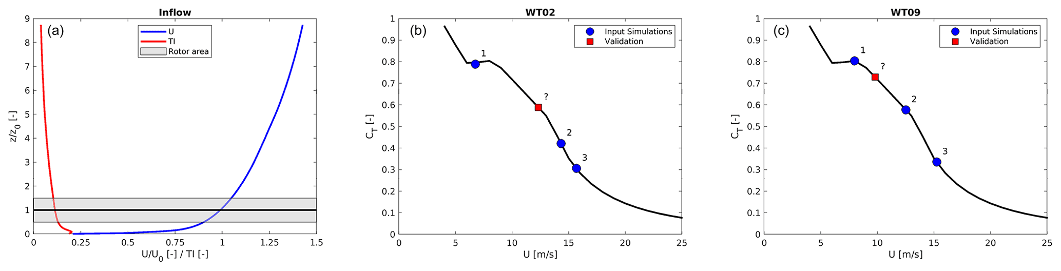
Figure 2 (a) Normalized and averaged streamwise velocity and turbulence intensity profiles; steady-state C_T curve and C_T values (b) for the wake-generating first turbine and (c) for the wake-generating eighth turbine in the input simulations and validation case in blue and red, respectively.

The neutral ABL precursor corresponds to a rough-wall boundary layer for high Reynolds numbers, and therefore the precursor flow can be re-scaled to create a number of different inflow conditions; see Castro (2007). The re-scaling yields a “new” velocity field based on the following formulation:

$$\begin{array}{}\text{(7)}& u^{\mathrm{new}}=u_{*}^{\mathrm{new}}\left({\displaystyle \frac{u^{\mathrm{org}}}{u_{*}^{\mathrm{org}}}}+{\displaystyle \frac{\mathrm{1}}{\mathit{\kappa }}}\ln {\displaystyle \frac{z_{\mathrm{0}}^{\mathrm{org}}}{z_{\mathrm{0}}^{\mathrm{new}}}}\right),\end{array}$$

where κ=0.41, and the original flow field is denoted by superscripts “org” (Troldborg et al., 2022).

4.1.2 Wind farm

The precursor flows are applied on the inlet boundary condition for the wind farm simulations, which have been performed on a new grid. The new wind farm grid is $L_X\times L_y\times L_z=\mathrm{7687.68}$ m × 800.8 m × 800.8 m, corresponding to $\mathrm{192}R\times \mathrm{20}R\times \mathrm{20}R$ in the streamwise, lateral, and vertical directions. The grid is equidistant from the inlet and in the vicinity of the turbines with a resolution of 20 cells per blade radius and stretched towards the lateral, top, and outlet boundaries. The resolution is quite high for actuator disc simulations, and the resolution is expected to give an error of less than 1 % in C_T (Hodgson et al., 2021). The grid has $\mathrm{3392}\times \mathrm{192}\times \mathrm{128}\approx \mathrm{83}\times {\mathrm{10}}^{\mathrm{6}}$ grid cells. Cyclic boundary conditions are imposed on the lateral boundaries to mimic an infinitely wide wind farm.

The 14 turbines are spaced 12R apart in the streamwise direction and 20R in the lateral direction, due to the cyclic boundary conditions. The modeled turbine is the NM80 turbine with a radius of R=40.04 m and a hub height of z₀=80 m. The turbine is re-scaled to a rated wind speed of U_rated=14 m s⁻¹ with corresponding rated power of P_rated=2750 MW.

4.1.3 Flow cases

The flow re-scaling is utilized in order to create a database, which covers a significantly reduced parameter space, where the thrust coefficient C_T is the only governing parameter. The inflow is re-scaled to have the same turbulence intensity and shear exponent for all flows, while only the inflow velocity at hub height varies and gives rise to differences in C_T for WT02 and WT09. The roughness (z₀=0.051 m) is calibrated to give an average shear exponent over the rotor area of α=0.14, which implies a turbulence intensity of TI≈11 % at hub height for all simulations, as all turbulence is mechanically generated for a neutral boundary layer. The friction velocity is calibrated to give inflow hub height velocities of U₀=8, 15, and 20 m s⁻¹ at the position of the first turbine. Additionally, a validation simulation has been run with inflow hub height velocity of 12 m s⁻¹.

The normalized inflow velocity and turbulence intensity profiles are shown in Fig. 2a, which also shows the steady-state C_T curve of the NM80 in Fig. 2b and c. The average C_T values of the first and eighth turbine for the three input simulations are marked with blue circles, while the validation simulation is marked by a red square.

The flow is initially developed throughout the wind farm for 1800 s to remove any transients from the simulations. All cases have been simulated for 13 107 s (3.64 h). The long simulation time is necessary in order to capture low frequencies and to generate a significant amount of data for comparing the stochastic generation. A visual impression of the highly complex and turbulent wind farm flow is given in Fig. 3, which shows streamwise velocity and iso-surface of the vorticity. The three velocity components – u, v, and w – are extracted in planes 1R upstream each turbine (as indicated) every 10 Hz, corresponding to 2¹⁷=131 072 snapshots. The extracted planes cover ±1.1R in the lateral and vertical. Here, the inflow to turbines 2 and 9 will be used to build PS-ROM, i.e., the wake generated by the first and the eighth turbine. The two cases showcase the generic capabilities of the model to capture single wake dynamics, and the inflow to the ninth turbine is arbitrarily taken as representative of deep wake conditions, where the statistical moments have generally converged (Andersen et al., 2020). Instantaneous snapshots of the streamwise velocity fluctuations are shown in Fig. 4, where the dynamics of the turbulent wake are clearly evident.

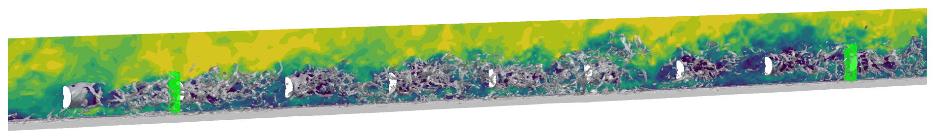
Figure 3 Vertical plane of streamwise velocity as well as iso-surface of the vorticity through a wind farm. Turbines are marked in white circles, and planes for extracting inflow velocity components for WT02 and WT09 are shown in green.

Figure 4 Instantaneous snapshots of the streamwise velocity fluctuations in a wake with C_T=0.806.

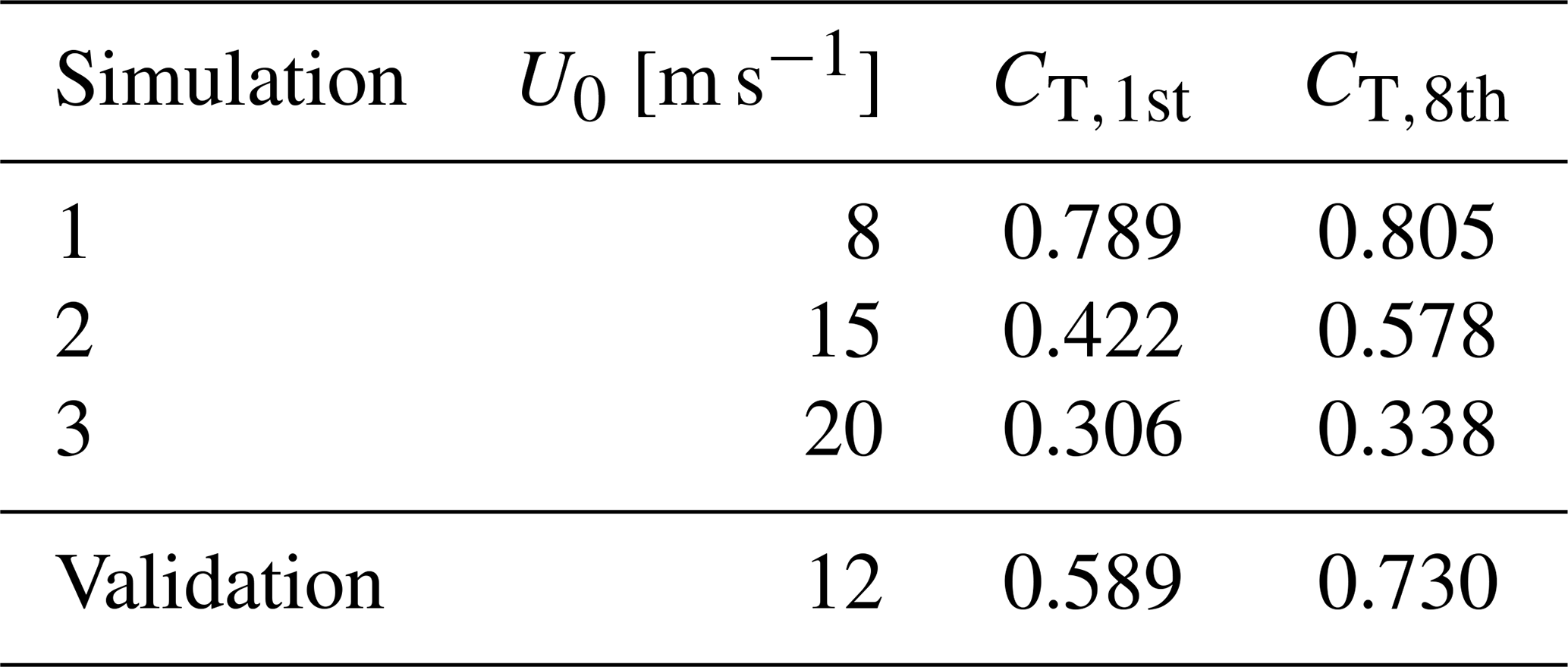
Table 1 summarizes the inflow parameters for the wind farm simulations and the operational conditions of the wake-generating first and eight turbine. The validation case is chosen to show the predicting capabilities of the model, as the C_T values of the two validation cases are located almost midway between two of the input simulations, i.e., the largest distance from simulated flows in the database. This is the case for both WT02 and WT09, although the distance from the validation cases to the input cases differs.

Table 1 Summary of inflow parameters for wind farm simulations and operational conditions of the wake-generating first and eighth wind turbines.

4.2 Global POD modes and modal time series

The global POD modes are computed using the database of inflows, where every 100th snapshot is used. The first 15 modes for the ninth turbine are shown in Fig. 5. Clearly, large structures are visible, which gradually diminish in size with increasing mode number, e.g., the monopole structure in mode 1 (and 9 and 11). Overall, these global and spatial POD modes are very similar to previously reported POD modes based on individual scenarios of either single wakes (Sørensen et al., 2015; Bastine et al., 2018) or multiple wakes (Andersen et al., 2013). The global POD modes for the inflow to WT02 is very similar but not shown for brevity. This clearly indicates how the dominant coherent structures are similar across cases and yields the potential for deriving a ROM based on such generic building blocks.

Figure 5 First 15 global POD modes, u component; note that each mode also has v and w fluctuating velocity components.

Figure 6 Modal time series of the first five global POD modes for WT02 and WT09.

However, the importance of each mode will differ from case to case. The original non-normalized flows are therefore re-projected into the global POD modes to obtain modal time series of each mode for each C_T value. The time series are shown for the first five modes of both WT02 and WT09 in Fig. 6. Low-frequency fluctuations are predominantly visible for the first mode for both WT02 and WT09 and to some degree in the second modes, but they effectively disappear for higher modes. Combined with the monopole structure of the global POD modes, this shows how the first mode is mainly a low-frequency correction to the mean velocity profile. Overall, the amplitude of the modal time series decreases for increasing mode number for all three cases. This can also been seen in Fig. 7, where the variance of the modal time series is plotted. The variance is a proxy of the turbulent kinetic energy in the modes, and the decreasing trends are very similar to the standard decrease in energy content of the POD eigenvalues, which shows how the global set of POD modes is a good basis for capturing the various flow scenarios for changing C_T. Some differences arise, in particular between the single wake inflow to WT02 and the deep array wake at WT09. The minor deviations from non-monotonic decrease indicate how the importance of different modes changes across the parameter space – for instance, the second global mode shows slightly higher variance than the first global mode for high C_T values. The contribution of variance is higher across all modes for the high C_T for WT02, which could indicate that more modes are required to fully capture the flow physics. The variance across modes is very similar for the smaller C_T values. This trend is also seen for WT09, where the variance is comparable although slightly lower for the lowest C_T.

Figure 7 Variance in each modal time series for WT02 and WT09.

The turbulent wake flow is highly non-linear, but POD is a linear combination of spatial modes and its corresponding modal time series. Therefore, non-linearity of the flow might emerge through the modal time series and their interaction, for instance correlation. Figure 8 shows the correlation of the temporal coefficients of the first 15 POD modes for WT02 and WT09, where the diagonal is obviously unity. Generally, the off-diagonal correlations are very small. However, several interesting aspects become apparent. There are clear modal interactions in the modal time series. The correlations tend to transition as C_T changes; e.g., modes 1–2 are negatively correlated for the lowest C_T of WT09, uncorrelated for the intermediate, and positively correlated for high C_T. Similar trends are observed for WT02. However, for WT02 the correlations are generally higher for modes 5 and above, while the modal time series are mainly correlated for the first five modes for WT09. Interestingly, the correlations are basically non-existent for the intermediate C_T value for both WT02 and WT09.

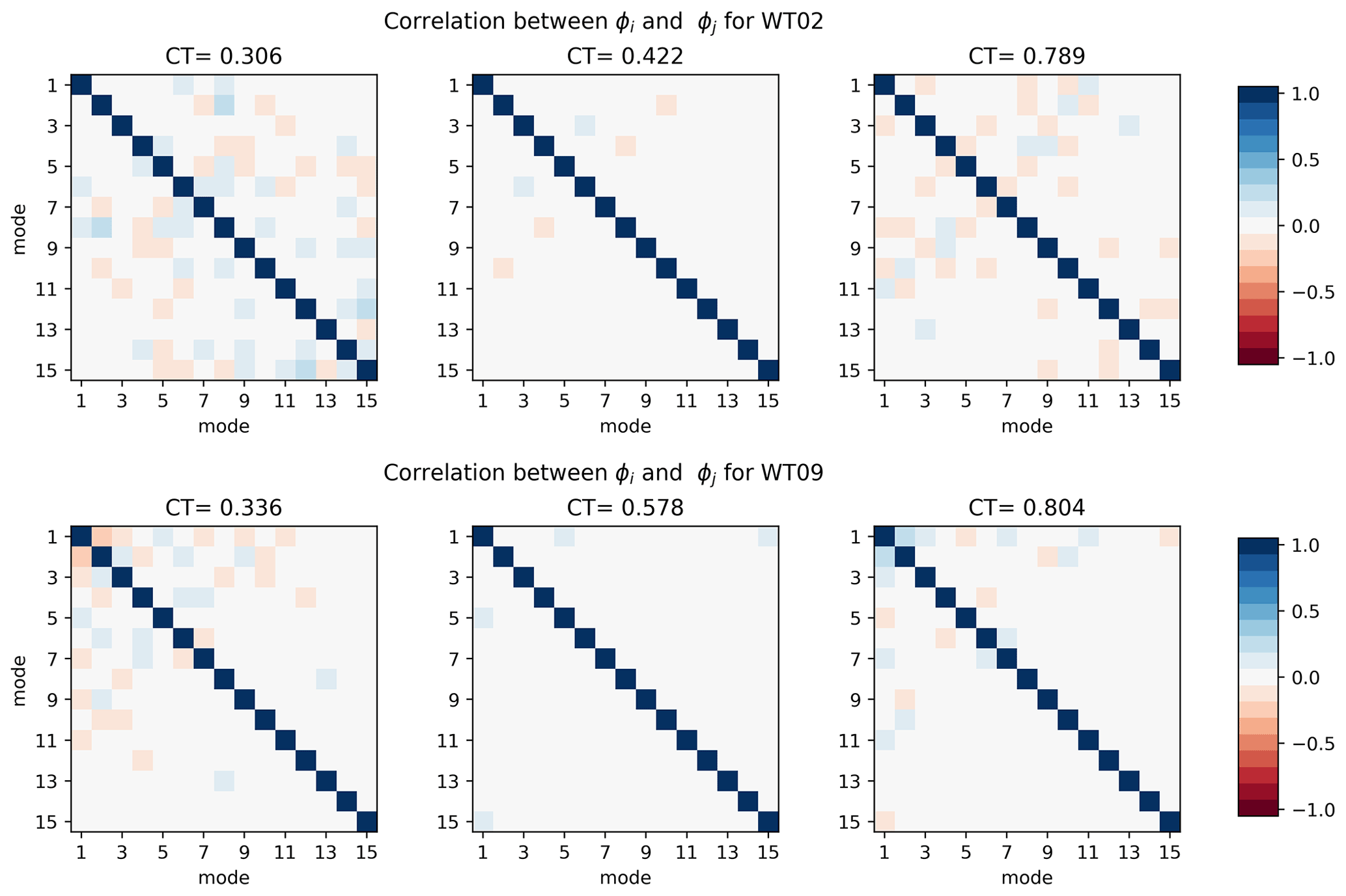
Figure 8 Correlation of the modal time series of first 15 global POD modes for the three C_T values for WT02 and WT09.

4.3 Cross-spectral density and stochastic generation

The temporal interaction of the different modes can also be examined through the cross-spectral density (CSD), which represents the covariance between multiple time series across the frequency spectrum. The CSDs are complex, but the norm of the filtered CSDs is shown in Fig. 9 for the first two modes.

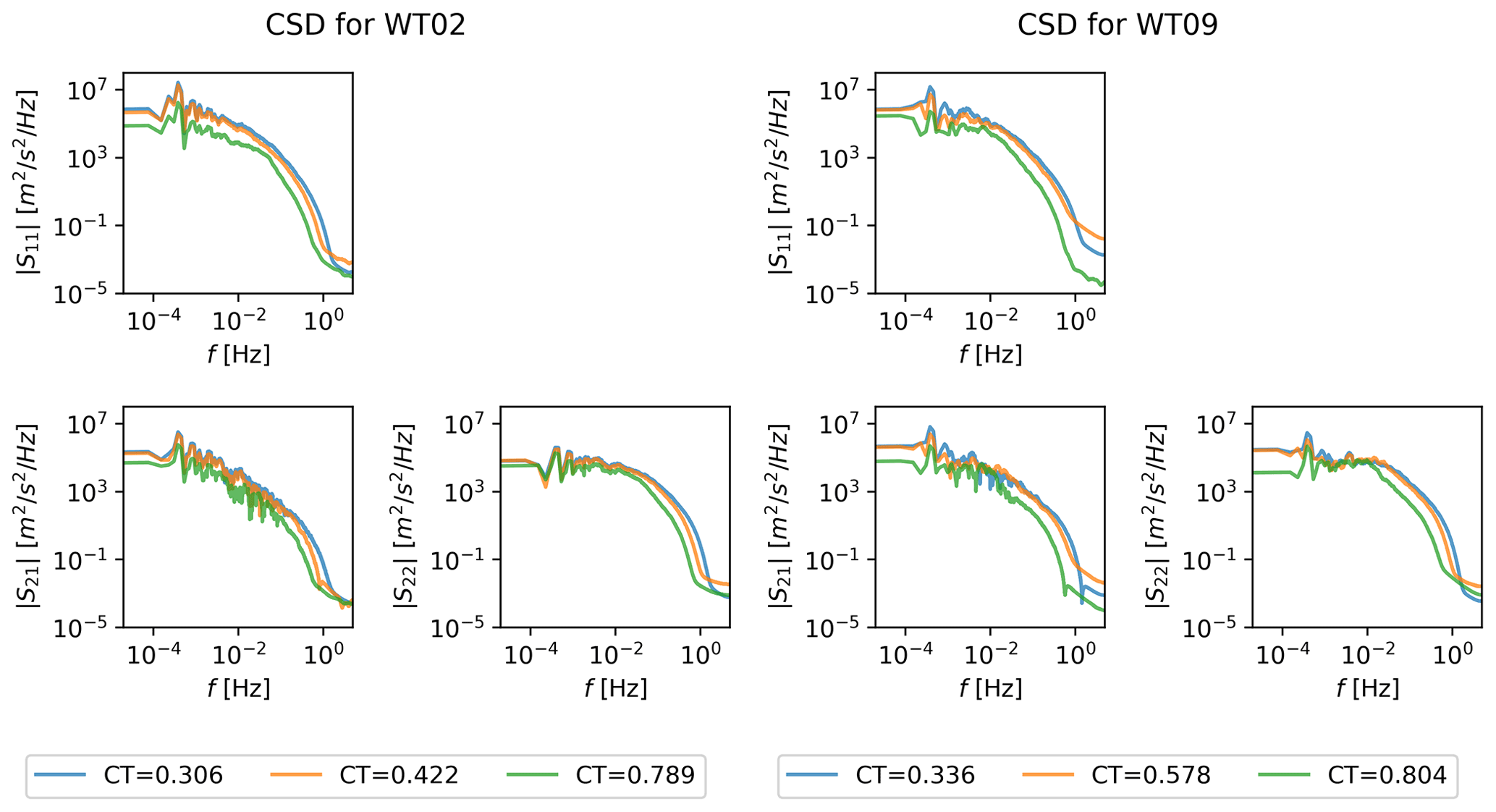
Figure 9 Norm of cross-spectral density of modal time series of the first two global POD modes for three C_T values and for WT02 and WT09.

The different C_T values affect both high- and low-frequency content across modes, and the kinetic energy is less for high C_T over the entire spectrum as expected due to the lower free-stream velocity. The energy content also decreases as the mode number increases. Some low-frequency interaction is generally present for the shown modes, although it is altered significantly for the high C_T in deep array. The norm of the CSDs is otherwise very similar across mode numbers.

Stochastic multivariate time series are generated from the complex CSD. Figure 10 compares the original CSD norm with the CSD norm of 20 randomly generated multivariate time series. The resulting CSDs are clearly very similar to the original for all modes and across the entire spectrum. Some spread from the random realizations is seen, which is expected and desirable.

Figure 10 Comparison of CSD of original and stochastic realizations evaluated at high C_T (a member of the training dataset) for WT02 and WT09.

The histograms of the original modal time series and of the 20 random realizations of the time series are compared in Fig. 11. The histograms are overall in excellent agreement, again showing that the random realizations capture the statistics of the original signal. The histogram are generally Gaussian for WT02, while the original histograms are slightly skewed for the first couple of modes for WT09 compared to the normally distributed random time series.

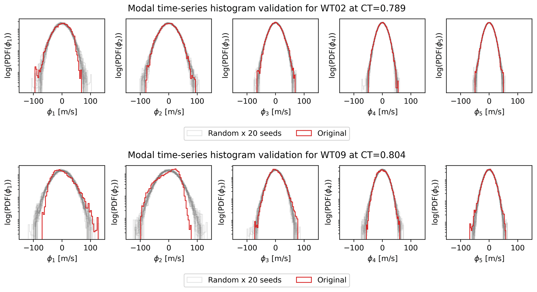
Figure 11 Comparison of modal time series histograms for original and random-realization-evaluated high C_T (a member of the training dataset) for WT02 and WT09.

4.4 Predicting out-of-sample flow cases

The stochastic capability of the reduced-order model needs to be supplemented by predictive capability for unseen cases, i.e., predicting wake dynamics for C_T values different from the three input simulations in Table 1. Here, a validation case is included with C_T values between simulation 1 and 2.

Stochastic realizations of the multivariate modal time series are predicted by interpolating the CSD at an out-of-sample C_T value. Here the CSD surrogate, $\widehat{\mathbf{S}}(f,\mathit{\theta })$, consists of a direct interpolator of CSD as a function of C_T, see Fig. 9, which clearly shows the dependency of spectral variance on C_T. Figure 12 shows 20 random realizations compared to the validation data. The agreement is excellent across the entire spectrum and for all mode numbers. Again, the random realizations show a spread around the validation CSDs.

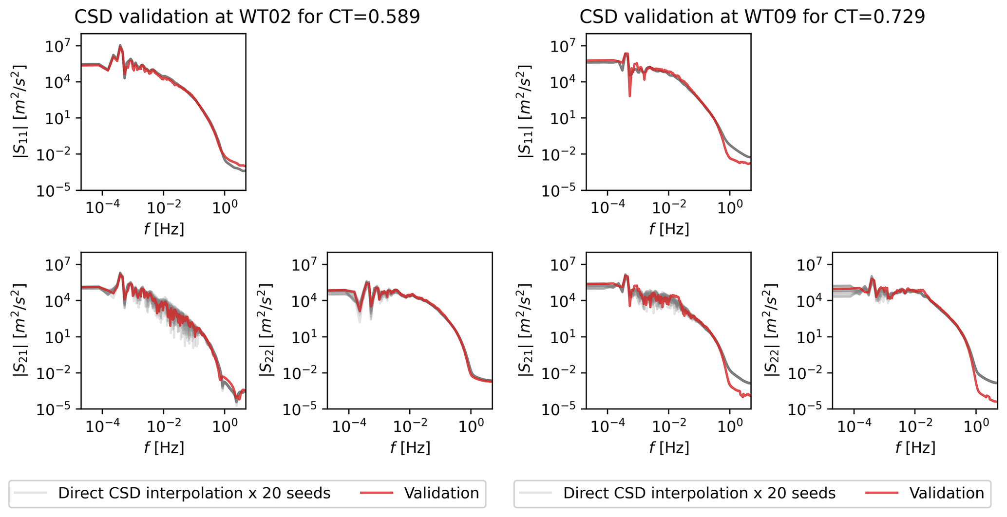
Figure 12 CSDs of 20 realizations of the PS-ROM using direct interpolation compared to the validation CSD for WT02 and WT09.

The dynamic wake inflow can now be reconstructed for each realization of the modal time series to compare with the validation simulation. Figure 13 shows a random stochastic realization using 50 modes, where the dynamics are clearly seen for different instantaneous snapshots.

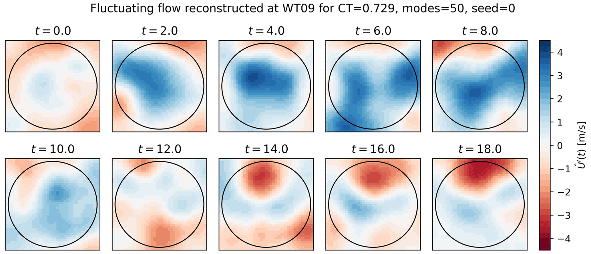
Figure 13 Instantaneous snapshots of the stochastic realizations of the streamwise velocity fluctuations in a wake with C_T=0.729 predicted with PS-ROM using 50 modes.

4.5 Model validation

The model is validated by comparing results of aero-elastic (Flex5) computations using both the original LES inflows and 100 random realizations generated by PS-ROM. The generated time series are 13 107 s long for both the original LES and the PS-ROM realizations. The realizations are split into periods of 650 s, which have an overlap of 300 s. Therefore, the LES dataset contains 42 statistical samples, while the 100 random seeds of PS-ROM yield a total of 4200 samples. Statistics are based on 10 min, including mean power and 1 Hz damage equivalent loads (DELs) for the main load channels of blade root flapwise bending moments (BRF), tower bottom fore–aft bending moment (TBF), and tower bottom side–side bending moment (TBS). The turbine will effectively act as a spatial filter, so higher modes with small scales can eventually be neglected.

Figure 14 shows violin plots of mean power and 1 Hz DEL of BRF, TBF, and TBS for PS-ROM realizations using 5, 10, 20, and 50 modes compared against the original LES inflow (red) for both WT02 and WT09. Generally, the distributions from PS-ROM are Gaussian, and it is clearly seen how the mean and width of the distributions increase as more modes are added to the flow generation, in particular for the DELs. It is expected that the stochastic generation of PS-ROM will result in wider distributions for most quantities as there are 100 times as many realizations, provided that a sufficient number of modes are used for the flow generation. Importantly, the distributions are clearly bounded.

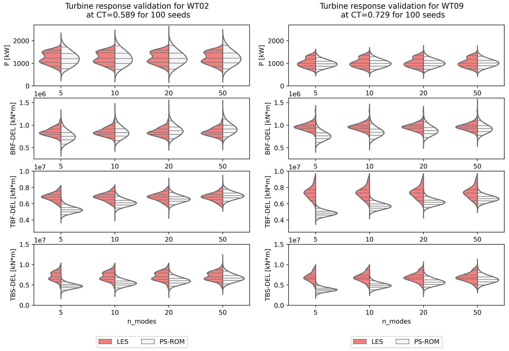
Figure 14 Distributions of 10 min mean power and 1 Hz damage equivalent load (DEL) of blade root flapwise (BRF), tower fore–aft (TBF), and tower side–side (TBS) bending moments for LES and for PS-ROM with 5, 10, 20, and 50 modes. Prediction at validation case, not used in the training of PS-ROM. Horizontal lines corresponds to 5th, 25th, 50th, 75th, and 95th percentiles. The statistics from PS-ROM is based on 100 random realizations of time series of 13 107 s long corresponding to 2¹⁷ flow snapshots. WT02 is shown on the left and WT09 on the right.

The median and quartiles (25 % and 75 %) of power are captured very well by PS-ROM for both turbines, although the LES validation dataset is non-Gaussian and with two distinct peaks. The PS-ROM distributions and therefore the extreme percentiles (5 % and 95 %) are wider in power for WT02 than for the validation LES dataset but are very comparable for WT09. Similarly, the distributions of BRF are also well captured, although it requires more than 10 modes for WT02 and more than 20 modes for WT09. The distributions of tower DELs are initially more sensitive to adding more modes, in particular the tower bottom bending moments. Adding more modes significantly increases the median and width of TBF and TBS, so they match the validation distributions very well for more than 20 modes. TBF for WT09 shows the worst comparison, where the PS-ROM realizations underpredict compared to the LES validation distribution. However, it is noteworthy how the LES distributions are very wide for WT09, arguably due to the increased turbulent wake dynamics in the deep array, which might require more modes.

Overall, the statistical comparison is very good, and it appears that 20 modes or more are generally sufficient to capture the distributions of power and the dominant loads. Obviously, the turbine acts as a spatial filter, which makes the flow generation more efficient as fewer modes are required (Saranyasoontorn and Manuel, 2005; Andersen, 2013). It is substantially fewer modes than previously reported by Andersen (2013), although the stochasticity helps to yield the correct statistical distributions.

5 Discussion

5.1 Assumptions, limitations, and advantages

PS-ROM is initially intended for dynamic wake simulations in order to quickly assess power and loads on wind turbines operating in wake, which requires accurate and fast flow generation. The computational time of generating new time series of 2¹⁷ snapshots is approximately 1–2 min using a Python implementation and depending on the number of global POD modes (and computing architecture, Sophia HPC Cluster, 2022), i.e., more than a 100 times faster than real time. For comparison, the execution time for generating a Mann turbulence box of comparable dimensions ($\mathrm{32}\times \mathrm{32}\times {\mathrm{2}}^{\mathrm{17}}$) is 6 min for a Fortran implementation. DWM requires generation of two Mann boxes, filtering and combining the different submodels, so timing is significantly longer. Each LES simulation required a total of approximately 39 000 CPU hours. Hence, PS-ROM is orders of magnitude faster than the alternatives, while also providing statistical distributions including the extreme estimates with high-fidelity LES accuracy.

The high accuracy is a significant advantage of PS-ROM compared to engineering models, such as DWM, with simplified physics and which are typically highly parameterized and therefore require calibration, e.g., Reinwardt et al. (2021). A particular critical assumption of engineering wake models relates to the superposition of individual single wakes to obtain flow inside wind farms. Numerous methods exists (Porté-Agel et al., 2020), but the models are particular sensitive around rated wind speed, where models typically switch binary between different methods, although the changes in C_T are continuous. This naturally affects the load predictions of such models (Larsen et al., 2017). PS-ROM inherently captures multiple wakes and the change from one control regime to another, e.g., from below-rated to above-rated wind speed.

PS-ROM also has certain limitations related to the assumptions of the model components. First, it requires sufficient data to resolve low frequencies and to satisfy the assumed stationarity and ergodicity required for the multivariate Gaussian process. Furthermore, the clear non-Gaussianity of the original LES dataset is challenging to capture and will require additional steps to generate non-Gaussian modal time series; see Fig. 11. Whether the stochastic generation will give rise to the same variability remains unknown, although the distributions indicate that the tails of power and DEL are captured very well. Second, the presented implementation of PS-ROM only predicts the turbulent fluctuations and therefore relies on knowing the mean flow across the parameter space. The mean wake flow can in principle be determined from an engineering wake model (e.g., Porté-Agel et al., 2020), RANS-CFD (e.g., van der Laan et al., 2019), or developing a surrogate of the mean flow based on the LES (e.g., Zhang et al., 2022). Third, the flow fields are extracted 1R upstream of the turbines and therefore include the effect of induction directly. Hence, PS-ROM does not incorporate changing control of the wake-affected turbine, e.g., individual pitch control or yaw misalignment. However, the induction at 1R upstream is essentially independent of turbine-specific details for the same C_T (Troldborg and Meyer Forsting, 2017), so it is assumed to only have minor influence. The low-frequency content of the generated turbulent fluctuations can in principle be corrected for induction (Mann et al., 2018) as well as corrections to the mean velocity due to induction (Troldborg and Meyer Forsting, 2017). As the model is assumed to essentially be independent of the specific wind turbine model, it is also expected that the model can be scaled geometrically for different turbine sizes operating at the same C_T (van der Laan et al., 2020).

Scaling the model significantly expands the generality of PS-ROM and the range of applications. As shown, PS-ROM is faster than DWM and yields loads and power distributions with LES accuracy. Therefore, PS-ROM can be applied similar to DWM to generate load surrogates of wind turbines operating in wind farms (e.g., Dimitrov, 2019) and hence used for wind farm plant design. PS-ROM can also be used to improve control algorithms of individual turbine controllers to be specifically designed to operate in wake dynamics as opposed to the present practice of tuning wind turbine controllers for free-stream conditions.

PS-ROM is currently limited to cover only the one parameter space of C_T. However, the stochastic nature, LES accuracy, and predictive capabilities across the parameter space effectively imply that PS-ROM can be viewed as a generalization of LES for statistically stationary flows. This has immense impact for the application of high-fidelity LES in general and not only for wind farm flow applications. Hence, PS-ROM can boost and enhance the value of a few LESs beyond the case-specific cases and thereby reduce the effective computational resources required for achieving high-fidelity results of highly turbulent flows.

5.2 Flow physics

PS-ROM enables a consistent approach to explore the underlying physics governing highly turbulent flows. POD has traditionally been used to gain insights into the dominant coherent turbulent structures and associated with main flow features. However, such analyses have limitations in the sense that these structures can not be measured or seen independently but only discovered though POD. Eventually, the higher mode structures merely represent an optimal mathematical basis of the turbulent fluctuation in space without specific physical interpretation besides small-scale turbulence. PS-ROM provides global modes, which decrease in size with increasing mode number. The global POD modes clearly resemble spatial POD modes of individual cases, and although they might be sub-optimal in terms of capturing the energy compared to individual cases, they clearly show the power of using global POD modes across the parameter space to elucidate on the flow physics. Changes in the parameter space are captured in the modal time series, and significant transitions will effectively change the importance of the individual global POD modes. PS-ROM proves that it is possible to interpolate over relatively large distances in the parameter space to get the weight of individual global modes through the CSDs of the modal time series. This is in contrast to previous results indicating that information is only locally available and can not be extrapolated globally (Christensen et al., 1999), or by interpolating between modes derived from individual cases to capture transitions (Stankiewicz et al., 2017). Interpolation in the CSDs is conjectured to be more robust than interpolating in the transition between locally derived modes.

Figure 8 shows how the modal interaction changes in physical space, i.e., whether PS-ROM is built for WT02 or WT09. Clearly, the modal interaction is spread on a larger number of modes for the wake generated by the first turbine, where the atmospheric flow is highly influential on the wake dynamics. Further in the farm at WT09, the modal interaction predominantly occurs between the lowest modes. The correlations are a direct manifestation of non-linearities in the flow, as it shows that the modes are not independent. Therefore, the flow dynamics can not be separated and linearized, but they need to be solved collectively. Separation of scales and the associated linearization prevent methods from fully capturing the flow physics, e.g., DWM and various methods for Galerkin projection. Galerkin projection methods typically solve the Navier–Stokes equations independently for each POD mode, which does not guarantee stable or efficient results despite significant efforts to include the non-linearities (Xiao et al., 2019). Conversely, PS-ROM is a more empirical approach but ensures that the inter-scale non-linear interactions are maintained in the generated turbulent flows. The influence of C_T on the correlations between modal time series also offers interesting insights on transitions from low to high C_T values. Surprisingly, the non-linearities seem to vanish for the intermediate C_T values. This indicates that the flow is more linear as the modes are independent for flows, where neither the atmospheric nor the wake dominates.

Another significant transition in the wind farm flow is seen in Fig. 9. The low-frequency content is visible for all C_T values of WT02. However, for WT09 the low-frequency content of mode 1 is significantly reduced for high C_T=0.804. This corroborates the finding of Andersen et al. (2017), where the most energetic length scales are eventually seen to be limited by the turbine spacing; i.e., for high forcing the turbines can break up the largest atmospheric flow structures. The low frequencies remain in the second mode but are significantly reduced for WT09 compared to WT02. In contrast, it has implications for DWM, which assumes that the low frequencies of the atmosphere govern the low-frequency meandering throughout the wind farm.

5.3 Future developments and open questions

Future developments will extend PS-ROM to cover a multidimensional space in order to increase the application range even further. However, the parametric space is large, so the sparsity of the LES dataset will present its own challenges to overcome the “curse of dimensionality”. How to perform multivariate interpolation while enforcing the necessary Hermitian properties of the CSDs is an open question. Despite sparsity of high-fidelity datasets, the simulations might require insurmountable computational resources to derive the global POD modes. Alternatives to POD exist for deriving global spatial basis. Generic and theoretically derived modes, e.g., Fourier–Bessel functions, could also be used. Formally, these modes require the variables of the eigenvalue problem to be stationary or homogeneous (George, 1988), but such modes could in principle be used irrespectively. It would simplify the determination of the global basis but would also enforce significant constraints in terms of assumed symmetries. Hence, it could inherently enforce an assumption that vertical shear and veer only have a linear influence on the flow and could be removed by initially subtracting the mean. From Fig. 5 it is clearly not the case as the first mode is asymmetric and appears to be a low-frequency correction to the mean velocity. Alternatively, various machine-learning dimensionality reduction methods could be used, for instance autoencoders, which present a non-linear generalization of POD (Hinton and Salakhutdinov, 2006). Autoencoders can build ROMs for complex non-linear problems with higher accuracy compared to POD. However, autoencoders are computationally demanding and less general in the sense that the optimal autoencoder architecture could change every time a new parameter scenario is added. PS-ROM does not suffer the same limitations due to its simplicity, both conceptually and in terms of model architecture, which is essentially a one-layer model. Nevertheless, the use of autoencoders could potentially increase the accuracy in PS-ROM.

Therefore, the fundamental model framework of PS-ROM is conjectured to be applicable for a wide range of highly turbulent flows, beyond wind farm flows. As PS-ROM is data-driven, it only requires high-fidelity data resolved in time and space, and the model framework can therefore also be applied to large measurement databases.

6 Conclusions

A predictive and stochastic reduced-order model for turbulent-flow fluctuations in wind turbine wakes is presented. The model is constructed using a high-fidelity LES database of the turbulent inflow to turbines operating in a large wind farm. The thrust coefficient of the wake-generating turbine is the governing parameter of the flows. A set of global building blocks are derived by applying proper orthogonal decomposition to the combined database covering the parameter space. The modal time series are obtained by reprojection the original flow into the global modes. The modal time series and corresponding cross-spectral density show a clear dependency on C_T, which enables a direct interpolation in the CSDs. PS-ROM is therefore able to predict unseen cases and generate random stochastic realizations with the correct spectral statistics. The model is validated against an independent LES in terms of power and damage equivalent loads. PS-ROM yields very good agreement in the distributions, including the extreme estimates of the 5th and 95th percentiles.

A validated, fast, and truly dynamic wake model has a number of applications:

• full load distribution estimation – the fast creation of new realizations will allow the simulation of the complete load distributions for a given operating condition, i.e., achieve actual estimates of extreme loads, e.g., 95th percentile estimates;

• new control algorithms dedicated for turbines operating in wake – advanced controllers can be designed to include different operation depending on, e.g., turbulence intensity (Dong et al., 2021), but extensions could be made to incorporate the specific time and length scales of wake dynamics as captured by the present model;

• wind farm optimization including loads by using PS-ROM to construct load surrogates.

The proposed model also provides significant insights to the physics of highly dynamic wind farm flow. It reveals how the non-linear interaction of the global modes changes significantly for different values of C_T, where non-linearities are mainly present for low and high values of C_T. The high values of C_T are also seen to significantly alter and reduce the atmospheric low frequencies in the deep array. The predictive and stochastic nature of the reduced-order model framework can be seen as the generalization of LES beyond the case-specific cases. Additionally, the consistent physical modeling and analyses are expected to be generally applicable for statistically stationary and highly turbulent flows and not only wind farm flows.