the Creative Commons Attribution 4.0 License.
the Creative Commons Attribution 4.0 License.
 | 02 Dec 2022
Current and future wind energy resources in the North Sea according to CMIP6
Oscar García-Santiago
Alfredo Peña
We explore the changes in wind energy resources in northern Europe using output from historical to mid-21st century CMIP6 simulations and the high-emission SSP5-8.5 scenario. This study improves upon many assumptions made in the past. First, we interpolate the winds to hub height using model-level raw data; second, we use a large ensemble of CMIP6 models; third, we consider the possible wake effects on the annual energy production of a large wind farm cluster proposed for the North Sea. The common practice of extrapolating 10 m wind speeds to turbine height using the power law with a constant shear exponent is often a poor approximation of the actual turbine-height wind speed. This approximation can exaggerate the future changes in wind resources and ignore possible surface roughness and atmospheric stability changes. The evaluation of the wind climatologies in the CMIP6 models over the North Sea for the historical period shows good correspondence with measurements from tall masts and three reanalysis data points for 16 of the 18 models. Some of the models run at relatively high spatial resolution are as good as the reanalyses at representing the wind climate in this region. Our results show that annual mean wind speed and wind resources in northern Europe are not particularly affected by climate change in 2031–2050 relative to 1995–2014, according to a subset of 16 models in the CMIP6 collection. However, the seasonal distribution of these resources is significantly altered. Most models agree on reductions in the future wind in summer in a band that extends from the British Isles to the Baltic Sea and on increases in winter in the southern Baltic Sea. The energy production calculations show that summer energy production in a planned large wind farm cluster in the North Sea could be reduced by a median of 6.9 % during 2031–2050 when taking into account the wind farm wakes (that accounts for −0.7 %) and the changes in air density (that account for −0.9 %).
- Article
(9793 KB) - Full-text XML
- BibTeX
- EndNote


The harvesting of electricity from the wind plays a significant role among climate change mitigation options. Integrated assessment models (i.e. models that link the main features of society and economy with the biosphere and atmosphere into one modelling framework) estimate that by 2050 renewable energy sources must supply 52 %–67 % of the global primary energy to limit global warming to 1.5 ∘C with no overshoot (IPCC, 2022). Wind and solar sources could provide nearly half of the required renewable energy (IPCC, 2022). However, wind and solar power plants supplied, respectively, only 6 % and 3 % of the global electricity consumption in 2020 (IRENA, 2019). Fortunately, cost reductions in wind power technologies and wind farm construction have increased the economic attractiveness of wind farms in many regions (IRENA, 2019; Beiter et al., 2021; Wiser et al., 2021). Therefore, because of its mitigation potential and lower costs, the construction of new wind farms will likely accelerate in the coming decades.
However, climate change could impact the supply of renewable energy, including wind energy (Cronin et al., 2018; Yalew et al., 2020; Gernaat et al., 2021). Many countries currently plan significant wind power expansion, with global projections for installed wind capacity in 2040 of 2400–3320 GW onshore (from about 700 GW in 2020) and 342–562 GW offshore (from about 34 GW in 2020) (IEA, 2019; GWEC, 2020, 2021). As one particular example, in 2021, the Danish Parliament approved the construction of two energy islands: one offshore near the natural island of Bornholm in the Baltic Sea and a second as an artificial island in the North Sea. The turbines off the coast of Bornholm will have a capacity of 2 GW. The proposed North Sea Energy Island wind farm cluster will become one of the largest energy hubs in Europe, with a target of 10 GW installed capacity in 2050 (COWI, 2020). The energy production and the financial profitability of all new planned wind farms, including the two Energy Island clusters, are calculated using historical wind resources (COWI, 2020). Still, there is a probable threat that wind resources will change in the future due to climate change during the lifetime of a wind farm.
The study of future changes in wind resources is not a new subject. A systematic literature search conducted in early 2022 with the keywords “Wind Resources” and “Climate Change” returned nearly 90 peer-reviewed articles from 2005. These include the assessment of future wind resources at the global (Karnauskas et al., 2018; Zheng et al., 2019), regional (Devis et al., 2018; Chen, 2020), and local scale (Chang et al., 2015; Alonso Díaz et al., 2019). The most recent papers that study the projected changes in wind resources use the wind speed simulated by global climate models from either the Coupled Model Intercomparison Project Version 5 (CMIP5; Taylor et al., 2012), the newer CMIP Version 6 (CMIP6; Eyring et al., 2016a), or regional climate models such as CORDEX (Giorgi and Gutowski, 2015). The CMIP5/6 and CORDEX models have a spatial resolution of hundreds or tens of kilometres, respectively. All of the studies, except for two (Sailor et al., 2008; Wang et al., 2020), used the raw wind speed output from the climate model to estimate the power production of a single wind turbine and explore how this will change in the future. The raw climate model output over land nearly always underestimates the extractable wind resources because it does not correctly consider the full spectrum of atmospheric motions that modulate the wind near the Earth's surface. In addition, wind turbines and wind farms “shade” each other at a range of spatial scales when nearby (Barthelmie and Jensen, 2010; Nygaard, 2014). Wake effects are also ignored in all previous studies.
Earlier studies have made assumptions that do not hold when studying real-life wind farms. First, 60 % of the articles about future wind resources use the 10 m wind output from the climate model to diagnose the hub height (≈50–200 m) wind speed. About half of these use a power law with a constant shear exponent of for land and offshore areas. Such an approximation generally overestimates the hub-height wind speed over the ocean. It exaggerates future wind speed changes because such a shear exponent is typical of winds over grass areas at ≈30–50 m. Even when an offshore value of the shear exponent is used for wind extrapolation over the sea, the value is constant, ignoring that air temperature will likely increase and atmospheric stability could vary in time. Second, the aerodynamic characteristics of the land surface and their changes in space and time are also of utmost importance for wind resource assessment. For example, changes in wind direction, coupled or uncoupled with changes in land use, could affect wind resources by changing the relationship between the orientation of the dominant flow and the orientation of the orography and the coastline. This effect can be ignored offshore and away from coastlines but could be very important over the land (Dörenkämper et al., 2020). Third, a large portion of the previously mentioned articles used a small sample of climate models. For near-surface wind-related quantities, models often disagree on the sign of future wind changes (Karnauskas et al., 2018; Pryor et al., 2020); thus, useful predictions should rely on as many models as possible. Fourth, all published studies disregard the effect of potential changes in wind direction and how these changes interact with the layout of ever-larger wind farms and their wake losses. Most previous studies use the power curve from a single wind turbine disregarding any wake effects. Lastly, most studies identify climate change's impact on wind resources at periods far in the future, 2050 or 2100. This is relevant for theoretical studies, for example, integrated assessment models (Gernaat et al., 2021), but governments and wind farm developers are asking these questions for the near future, 20–30 years from now.
This study improves upon four of the five assumptions described above. First, we interpolate the winds to hub heights using model-level raw data. Second, we use all available CMIP6 models, which have all the necessary fields for the vertical interpolation of the wind speed at the highest output frequency (6 h). Third, we consider a huge wind farm proposed for the North Sea and investigate the role of the future changes in wind direction and wake losses. Finally, we assess climate change for the 20 years 2031–2050, not at the end of the century. We concentrate our study on a relatively small area of northern Europe, but this is where large wind farms already operate, additional development is planned, and data from tall offshore masts are available for verification of the winds in the reanalysis and climate models in the historical period. We ultimately demonstrate how a study of future climate changes in wind resources could be applied to a relatively small area and be helpful to energy planners and wind farm developers. The methods demonstrated here can be easily transferred to any other region offshore.
The paper is organized as follows. Section 2 describes the data from climate models, reanalyses, and tall masts used in the study. It also compares masts and reanalyses data to decide on an observed reference for the wind climate of the past. Section 3 describes the vertical interpolation and the verification metrics used in the study. The characteristics of the wind farm cluster used in the last part of the study are described in Sect. 3.3. We evaluate the various reanalysis against tall mast data and reanalyses against CMIP6 models for the historical period in Sect. 4. The results of the evaluation of wind resources in the future are shown in Sect. 5 for the North Sea. Section 6 presents the analysis for the future Energy Island wind farm cluster. We finalize with a discussion of the results in Sect. 7 and conclusions in Sect. 8.
2.1 CMIP6 models, simulations, and data
The CMIP project started 20 years ago as a platform to compare early coupled climate models (Meehl et al., 1997). The models being coupled were the global atmosphere, dynamic ocean and thermodynamic sea ice, and simple land surface models. These early models often required “flux adjustments” to keep their simulated climate from drifting when performing decade-long time integrations. The models used in CMIP6 have been improved, no longer using flux adjustments, and incorporate many other sub-models, including, for example, river runoff, sea ice dynamics, ocean waves, atmospheric chemistry, and models that explicitly predict natural CO2 concentrations via bio-geophysical cycles in the land and ocean biosphere. These sub-models are needed to carry on the CMIP6 project design to understand the response of the Earth's system to forcing and how we can assess future climate changes given the internal climate variability, predictability, and uncertainties in scenarios (Eyring et al., 2016b).
Table 1 describes the main characteristics of the CMIP6 models used in this study. Two general types of models are used in CMIP6 simulations that differ in treating natural CO2 concentrations. Earth system models (ESMs) account for the fluxes of CO2 between the atmosphere, ocean, and biosphere. In climate models (CMs, also known as atmosphere–ocean general circulation models, AOGCMs), changes in CO2 concentrations are prescribed and cannot vary in response to climate change. In both types, anthropogenic sources of CO2 and other greenhouse gases (GHGs) are prescribed. We use data from both CMs and ESMs with spatial resolutions that vary from coarse (2.81∘) to relatively fine (0.83∘ in longitude).
As far as is possible, the historical forcings are based on observations and cover the period 1850–2014. These include emissions of short-lived species and long-lived GHGs, GHG concentrations, global gridded land use, solar forcing, and stratospheric aerosols (e.g. volcano emissions). For models without ozone chemistry, time-varying gridded ozone concentrations and nitrogen deposition are also provided. For future climate simulations (2015–2100), CMIP6 also provided coordinated multi-model climate projections based on alternative scenarios of future emissions and land-use changes produced with integrated assessment models (O'Neill et al., 2016), which, in turn, are determined from future pathways of societal development, i.e. the Shared Socioeconomic Pathways (SSPs) (Riahi et al., 2017). The historical and future global climate model data were obtained from the CMIP6 DECK experiments; we use data from the historical simulations for the period 1980–2014 (1850–2014 is available for many models), and the SSP5-8.5 scenario for the period 2015–2050 (2015–2100 is available). In total, we downloaded a 70-year-long time series for all models.
We use data from climate simulations forced by the high end of the range of future pathways emissions, i.e. SSP5-8.5, with high enough anthropogenic emissions to produce a radiative forcing of 8.5 W m−2 in 2100. We chose to use this extreme scenario for two reasons. First, it might demonstrate the maximum expected impact on wind resources, and, second, it is the scenario with the most available data needed for this study. In the CMIP6 SSP5-8.5 scenario simulations, the forcing is specified as land use (fractions of crops, pasture, urban, and forest areas), emissions and concentrations of long-lived GHGs, air pollutants emissions, and short-lived forcing by gases (e.g. ozone). We use data from the near future, 2015–2050, because it could influence the planning and building of wind farms in the coming years. Some past studies have supplied changes for times further in the future, e.g. 2071–2100 (Jerez et al., 2019; Chen, 2020). However, wind farm developers are currently planning these farms and need data useful to assess the short-term future, i.e. during the expected lifetime of a wind farm.
The data used in this study are a particular set from the “6hrLev” table, which contains time series of zonal and meridional winds (u and v, respectively), air temperature (T), and specific humidity (q) on the original model levels and surface pressure (ps) every 6 h. The data are available from the Earth System Grid Federation (ESGF; Cinquini et al., 2014) database downloaded via OPeNDAP. To locate the desired dataset, we use the Python esgf-pyclient package (ESGF, 2022). The vertical structure of most models guarantees that wind data exist for levels below 100 m above ground level (a.g.l.) for all models and below 50 m a.g.l. for 14 of the 18 models. For this reason, we use winds at 100 m a.g.l., close to modern offshore wind farm hub heights.
Tilo et al. (2020)Swart et al. (2019)Danabasoglu et al. (2020)Cherchi et al. (2019)Voldoire et al. (2019)Séférian et al. (2019)Sellar et al. (2020)Sellar et al. (2020)Boucher et al. (2020)Tatebe et al. (2019)Hajima et al. (2020)Mauritsen et al. (2019)Müller et al. (2018)Kawai et al. (2019)Yang et al. (2020)Seland et al. (2020)Seland et al. (2020)Sellar et al. (2020)Table 1Models in the CMIP6 archive with u, v, T, and q available at model levels and 6-hourly output in the historical and SSP5-8.5 simulations. CM stands for climate model, and ESM stands for Earth system model.
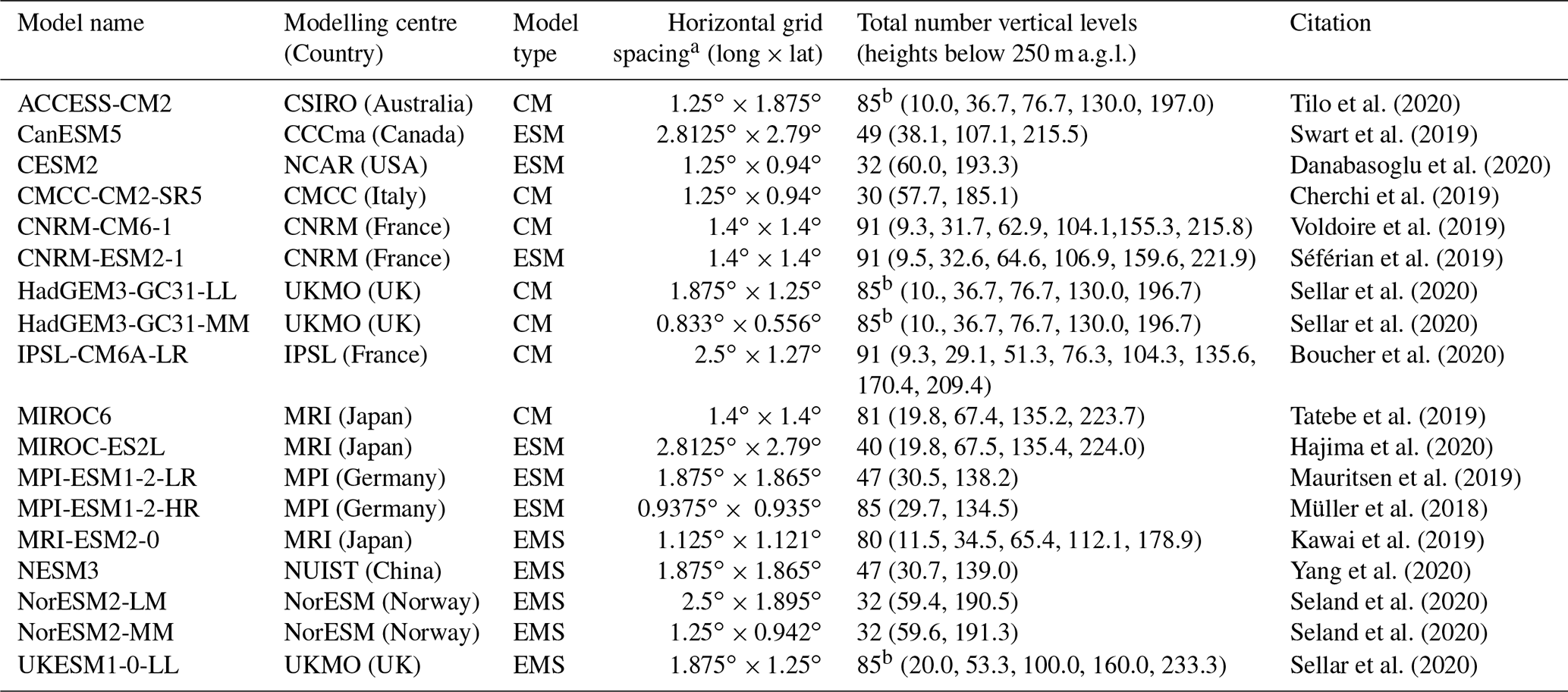
a Approximate value in the region because some models use Gaussian grid with variable latitude grid spacing. b Model data are already given in height above ground level.
2.2 Reanalysis and mast observations
We use the wind speed and direction derived from three modern reanalysis: ECMWF ERA5 (Hersbach et al., 2020); NASA Modern-Era Retrospective Analysis for Research and Applications, Version 2 (MERRA2; Gelaro et al., 2017); NOAA 20th Century Reanalysis version 3 (20CR; Slivinski et al., 2019); and the New European Wind Atlas (NEWA; Dörenkämper et al., 2020). Some general details for each dataset are listed in Table 2, including their advantages and disadvantages from a wind energy perspective. The wind speeds and directions from MERRA2 are interpolated to 100 m a.g.l. from the native model levels, similarly as to what was done with the CMIP6 data (this is described in Sect. 3.1).
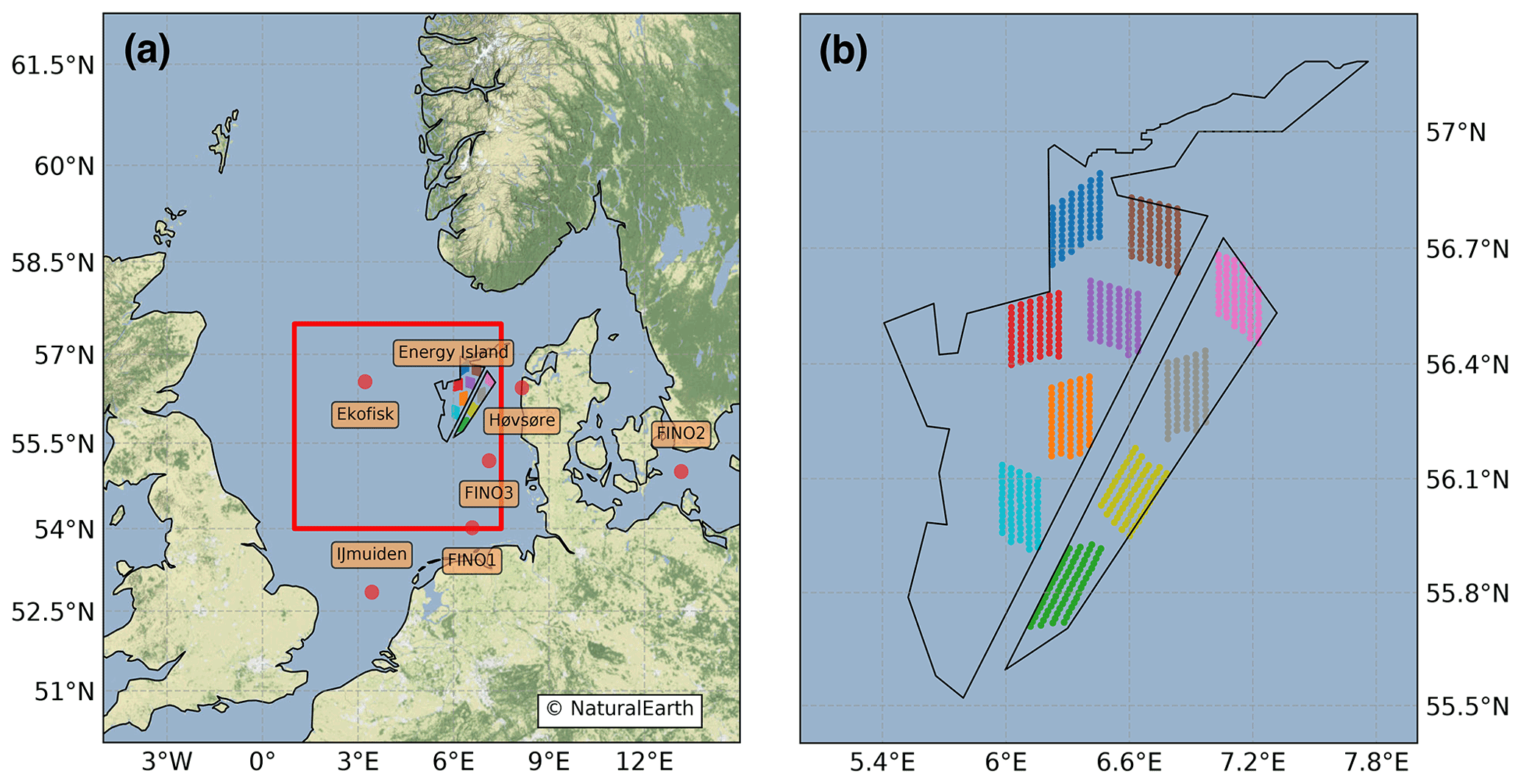
Figure 1(a) Location of the sites used for validation (red markers) and the area used for spatial averaging (red box). The area in black represents the layout of the Energy Island wind farm cluster. (b) Layout of the future Energy Island wind farm cluster area (black lines) and the 10 wind farms in markers with different colours.
Table 2Description of the various datasets used in the model evaluation of the historical wind climate.
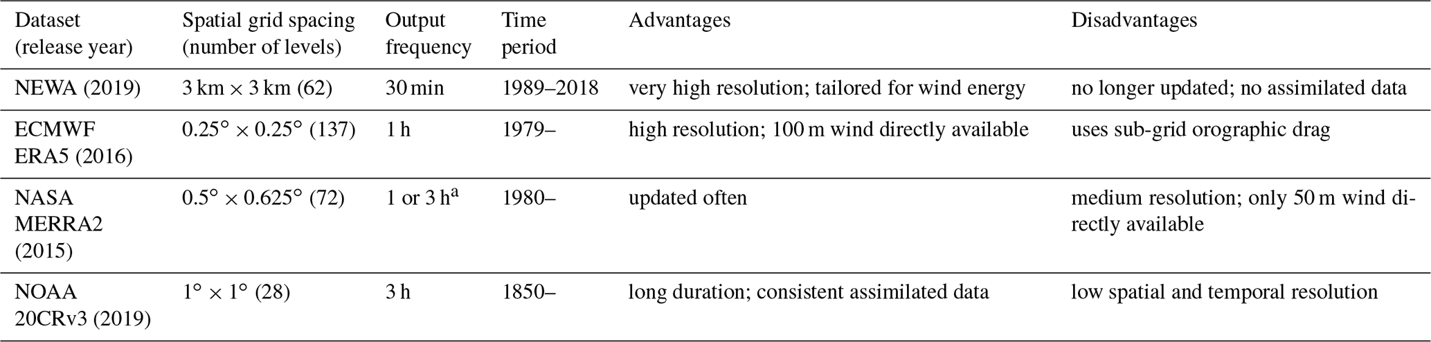
a MERRA2 50 m a.g.l. winds are available every 1 hour and atmospheric fields every 3 h.
We use data from six tall masts (Fig. 1a), with relatively long duration, in the North and Baltic seas to evaluate the boundary layer winds in the reanalysis datasets. The data are from offshore platforms (FINO1, FINO2, FINO3, IJmuiden, and Ekofisk) and a coastal met mast (Høvsøre) and are down-sampled to hourly from their original 10 min averages. When the site has various measurement levels, we select the highest and less-disturbed level as described in Hahmann et al. (2020). The data processing from the mast on the oil platform Ekofisk is described in Solbrekke et al. (2020). We use the data from the anemometer at 102 m above mean sea level. Figure 1a also shows the location of an averaging box (54–57.5∘ N, 1–7.5∘ W) used later in the future climate calculations and the location of the proposed Energy Island wind farm cluster.
3.1 Vertical interpolation of winds
The CMIP6 data from the various models are available via the ESGF database. The 6hrLev table contains the high temporal resolution atmospheric model data on pressure–sigma levels or heights above the model terrain. Thus, the wind speed and direction can be interpolated to any height above the first model level, which is listed in Table 1.
For the models with sigma coordinates, the pressure at model level k is computed from
where p0, ak, and bk are the reference pressure and the sigma level coefficients at level k and ps is the surface pressure. The thickness between two model layers, zk+1 and zk, can be determined from the hypsometric equation:
where
is the virtual temperature, which is averaged (therefore the overbar) between levels k and k+1, ϵ=0.622, Rd is the gas constant for dry air, and g is the Earth's gravitational constant. T and q are the air temperature (ta) and specific humidity (hus). The height of each model level can be obtained by integrating Eq. (2) from p=ps to the model level pressure p=pk. Knowing the height of each model level, the horizontal wind speed, , can then be interpolated to any height above the model terrain; u and v are the two wind components, named ua and va in the ESGF database. We use a linear interpolation in ln z for three heights: h=50, 100, and 200 m a.g.l. To obtain the wind direction ϕ at these heights, we linearly interpolate the two horizontal wind components in height separately and recalculate the resulting wind direction. The evaluation of the past and future wind climate is for a hub height of 100 m a.g.l.
The wind power density P is defined as
where ) is the surface air density and Tvs is the surface virtual temperature. Sometimes we use the air density for the standard atmosphere: ρst=1.225 kg m−3. We name the wind power density computed using the standard air density the standard wind power density Pst.
We also use the 10 m wind speed directly from the ESGF archive for comparisons. This field is named sfcWind in the daily and monthly data archive. As in previous studies, we use the power law to extrapolate from 10 to 100 m a.g.l.,
where . The implications of using the power law to extrapolate winds from 10 m instead of the vertical interpolation of wind speed from model levels are discussed later in the paper.
3.2 Model validation metrics
We use several metrics to evaluate the model simulations' accuracy compared to atmospheric reanalysis. The bias is a popular error statistic for comparing the wind speed distributions between observations and model-simulated fields. However, since the power density is a function of the cube of the wind speed (see Eq. 3), the shape of the wind speed distribution is more critical. Small changes in the wind speed distribution are amplified when converted to power, especially at the upper end of the distribution. Accordingly, we use the Earth mover's distance (EMD) to evaluate the differences in the shape of two frequency distributions (Hahmann et al., 2020). The EMD is equivalent to the area between the two cumulative distribution functions for one-dimensional distributions. The circular EMD (CEMD; Rabin et al., 2008) extends the EMD concept to one-dimensional circular histograms, such as the frequency distribution of wind directions. The smaller the value of EMD and CEMD, the better the distribution of the simulated wind speed and direction match those observed.
To diagnose the ability of the models to represent the annual cycle of wind speed, we compute the monthly mean of wind speed and then their average over the historical period ( and , where the subscripted o and m stand for the observed and modelled values and i=1…N is the month). To evaluate the annual cycle in wind speed in the CMIP6 model against that of the reanalysis, we compute the root-mean-square difference (RMSD) as
where N=12 months. We also use the EMD, CEMD, and RMSD to diagnose changes in the future wind climatology compared to historical conditions.
We use boxplots to compare wind speed distributions and other parameters among sites, reanalysis, and CMIP6 models. The boxplots in this paper show the “minimum”, first quartile (Q1), median, third quartile (Q3), and “maximum” of each distribution. The minimum and maximum are defined as Q1 −1.5 IQR and Q3 +1.5 IQR, respectively, and IQR = Q3 − Q1 is the interquartile range.
3.3 Wind farm energy production calculations
We perform annual or seasonal energy production calculations for the planned Energy Island wind farm cluster in the North Sea (Fig. 1b) using the time series of the past or the future wind speed and direction derived from the CMIP6 models and the reanalyses. The planned wind farm cluster consists of 10 wind farms, each having an installed capacity of 1 GW. The wind farm layouts (using a spacing of 7×12 rotor diameters D with D=240 m) in Fig. 1b come from the Energy Island report (COWI, 2020), consisting of 67 total 15 MW wind turbines for each wind farm layout. The turbine locations in each wind farm were digitalized by hand.
We use the engineering wake model of Jensen, as described in Göçmen et al. (2016), for wake calculations. This wake model accounts for the momentum (or velocity) deficit, which causes a reduction in the power output of the downstream turbines. The wake model superposes the individual turbine wakes by considering the wind direction and wake length. This wake model does not account for the mesoscale shadowing of one wind farm to another farm downstream. The wake model needs information on the thrust curve, rotor diameter, and the wake expansion parameter. The wake expansion is an empirical parameter that varies according to the wind farm, surface roughness length, and averaged atmospheric turbulence (Peña and Rathmann, 2014; Peña et al., 2016). We set the Jensen wake expansion parameter to 0.04, although this depends on turbulence, among other factors (Peña and Rathmann, 2014; Peña et al., 2016). We use the IEA 15 MW reference wind turbine (Gaertner et al., 2020) for the wind turbine characteristics. The wind turbines have a hub height of 150 m.
The power output for the wind turbines in the farm cluster is calculated every 6 h using the wind speed and wind direction from the ensemble of CMPI6 models and three reanalyses for the 10 wind farms. We also calculate the power time series at the highest frequency available for ERA5 (1 h), MERRA2, and 20CR (3 h) reanalyses to estimate the effect of the aggregation to 6 h in the CMIP6 models. The wake-free wind speed and direction time series, which are input into the wake model, are derived by vertical interpolation to hub height (z=150 m) and horizontal interpolation to the coordinates of the centre of the Energy Island cluster (56.4∘ N, 6.0∘ E, Fig. 1b). For simplicity and because of the smooth nature of the CMIP6 model output, we assume the wind speed and direction as horizontally homogeneous through the wind farm cluster, and thus it is only perturbed by the turbines' wake.
The energy production, EP, has units of gigawatt hours. It is calculated by summing up the 6 h energy output over all turbines within the analysed period or over a particular season within the analysed period. This also assumes that the energy output is constant over the 6 h. We perform three possible energy production calculations for the historical (1995–2014) and future (2031–2050) periods. The reference energy production, EPref, uses the nominal turbine power curve by multiplying it by the total number of wind turbines (no wake losses are included). The “standard EP”, EPst, includes wake losses but uses the standard density value. And finally, the net EP considers both the wake losses and variable air density. Wind farm yield calculations often include other technical losses, such as the availability of wind farms (some turbines may be offline due to faults), electrical efficiency, turbine performance, and curtailment. These losses are ignored in this study.
Since the mast measurements are at different heights, cover different periods and have various output frequencies than the CMIP6-derived winds, we evaluate the wind climatology from the CMIP6 historical simulations using a multi-step approach. We first compare the time series of mast measurements to reanalysis at the six sites at the highest possible time resolution. Once we demonstrate that these reanalyses are adequate, the CMIP6 evaluation is carried out using only the 6-hourly reanalysis data at the centroid of the Energy Island at a single level, 100 m a.g.l., but for the entire historical period (1980–2014), considering the wind speed and wind direction distribution, and the amplitude of the annual cycle in wind speed. To complete the wind climate evaluation, we survey the summary statistics (Sect. 3.2) for the sites in the North Sea and the Energy Island location. Lastly, we present the comparison of the EP calculations for the Energy Island.
Figure 2 shows the evaluation of the four different reanalysis (Table 2) against the observations for the six sites (Sect. 2.2). The reanalysis wind fields have been bi-linearly interpolated to the exact coordinates and height of the tall mast measurements. The data availability varies among the sites: from 15 years at Ekofisk to 4.5 years at IJmuiden. As illustrated, the four reanalyses represent the wind climatology very well both in terms of the mean wind speed (absolute biases <0.5 m s−1 at 75 % of the sites and reanalysis) and its distribution (except for 20CR). At the three sites that surround the Energy Island, Høvsøre, FINO3, and Ekofisk, the bias between the wind speed estimated by the ERA5 reanalysis and that observed are 0.04 %, −2.81 %, and −5.69 %, respectively. The 20CR wind speeds are lower than the observed wind speeds at all sites, especially at FINO2, which is influenced by the proximity to land in the Baltic Sea. To evaluate the CMIP6 simulations during the historical period, we continue with ERA5, MERRA2, and 20CR with a grid spacing comparable to the climate models.
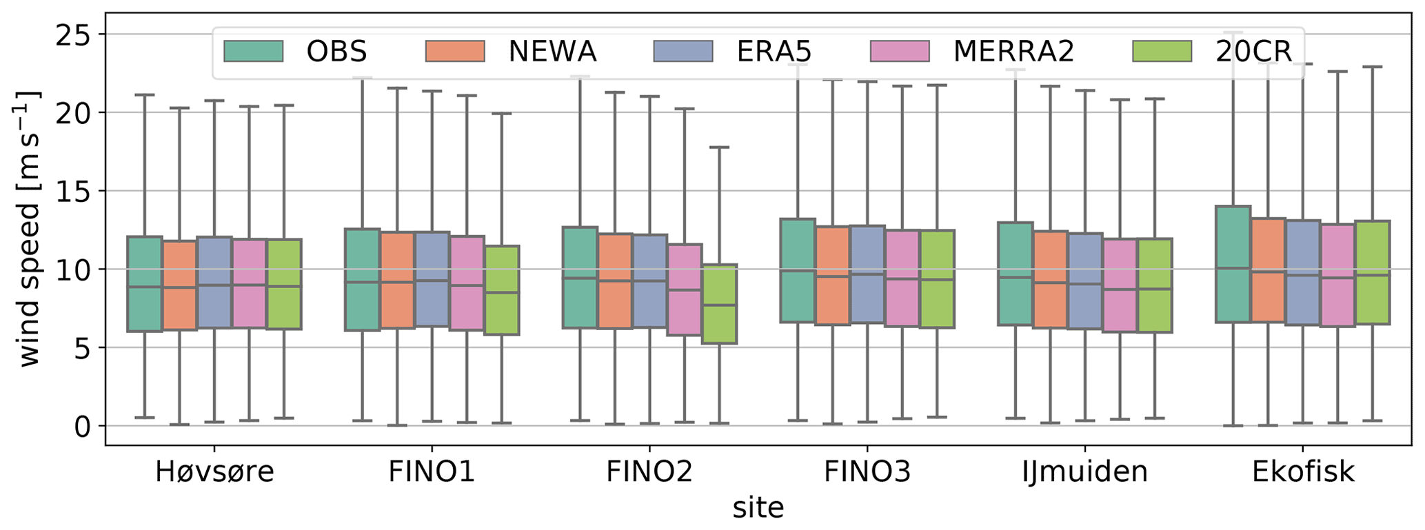
Figure 2Comparison of the observed and reanalysis-derived wind speed statistics at the six observed sites in Fig. 1a. The reanalysis and observations are synchronized in time and thus are at a 3 h frequency. The boxplots show the “minimum”, first quartile (Q1), median, third quartile (Q3), and “maximum” of each distribution.
4.1 The wind speed climatology at the Energy Island location
Figure 3 compares the 100 m wind speed climatologies among the CMIP6 models and the reanalysis for the time series at the centroid of the proposed Energy Island (Fig. 1) for the entire historical period (1980–2014). As previously demonstrated when comparing to the observed data (Fig. 2), the wind climate of the various reanalysis is nearly identical, with a mean of 10.0–10.2 m s−1. The wind climatology of the CMIP6 models is comparable to that of the reanalysis models, with mean values in the range of 9.1–10.7 m s−1. The exception is the two simulations using the MIROC model, with a mean of 8.1 and 6.3 m s−1, which is well outside the other models' range; it is not clear whether the MIROC model discrepancies are due to problems in the model simulation itself or the data provided in the ESGF archive. Comparing the 10 m wind speed for the two MIROC models against that of the other CMIP6 models (not shown) does not display such a large discrepancy. The median of most models is within ±1.5 m s−1 of that estimated by the three large-scale reanalyses. In general, the IQR in the CMIP6 models is slightly larger than that estimated by the reanalysis. The maximum wind speed, excluding any outliers, in the CMIP6 models is 20–25 m s−1, consistent within about 1–3 m s−1 with the three reanalyses, except for the MIROC and CanESM5 models.
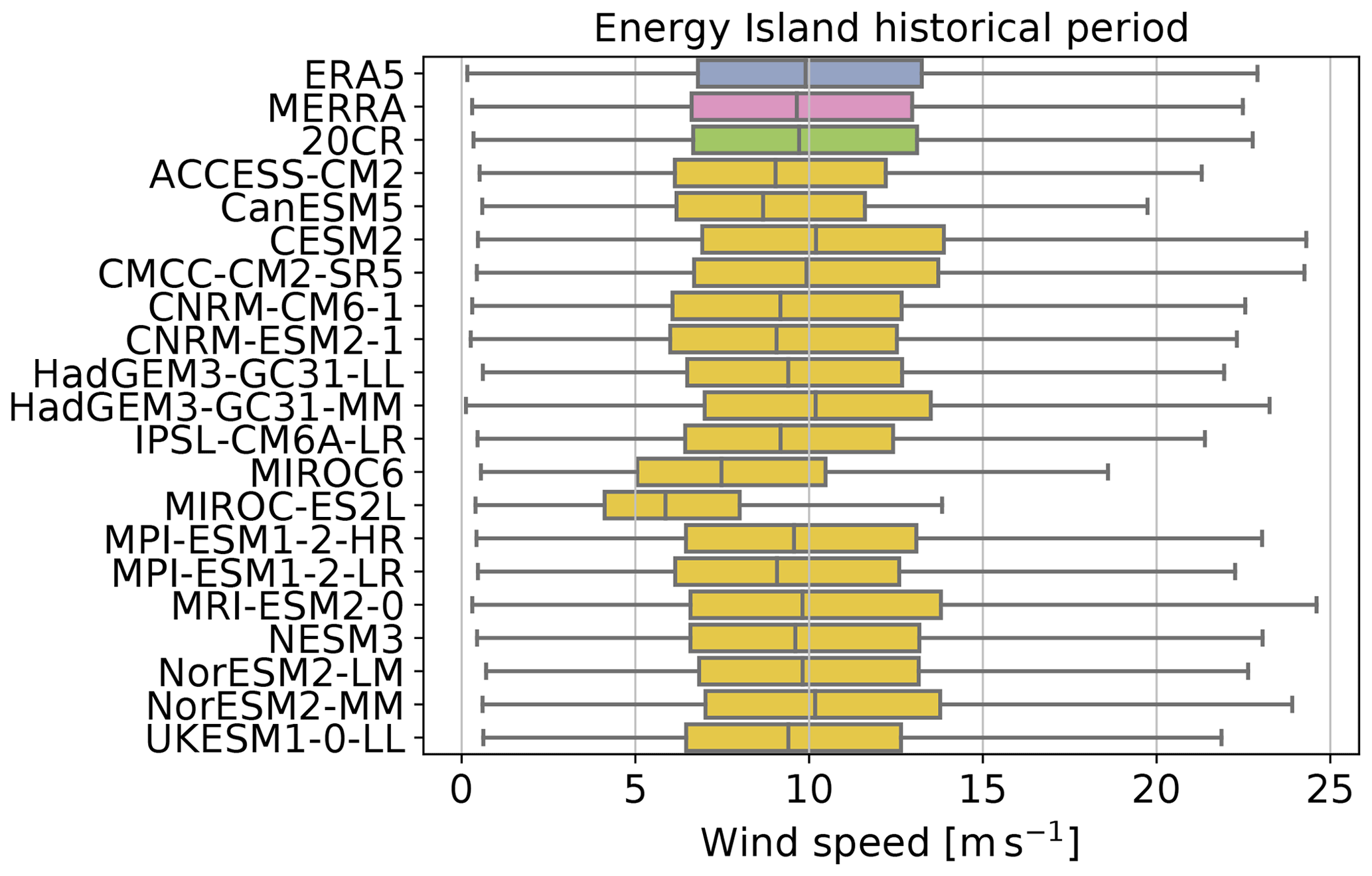
Figure 3Comparison of the wind speed at 100 m a.g.l. simulated by the CMIP6 models (see Table 1) and that provided by global reanalyses during the full historical period (1980–2014) for the Energy Island. The 6-hourly data from each CMIP6 model is synchronized with the ERA5 reanalysis. The boxplots show the “minimum”, first quartile (Q1), median, third quartile (Q3), and “maximum” of each distribution.
We also compare the combined wind speed and direction distribution (wind roses) for two CMIP6 models (i.e. the best and the worst) to the ERA5 reanalysis for the Energy Island. Figure 4 shows a remarkable similarity between the wind rose of ERA5 and the MPI-ESM1-2-HR model (CEMD = 3.8∘), but poor similarity between ERA5 and the coarse-resolution NorESM2-LM model (CEMD = 14.8∘). All models represent the dominant SW to NW flow in various degrees (not shown). Further analysis for all models and sites is done later in this section (see Fig. 6c for all CEMD for all models).
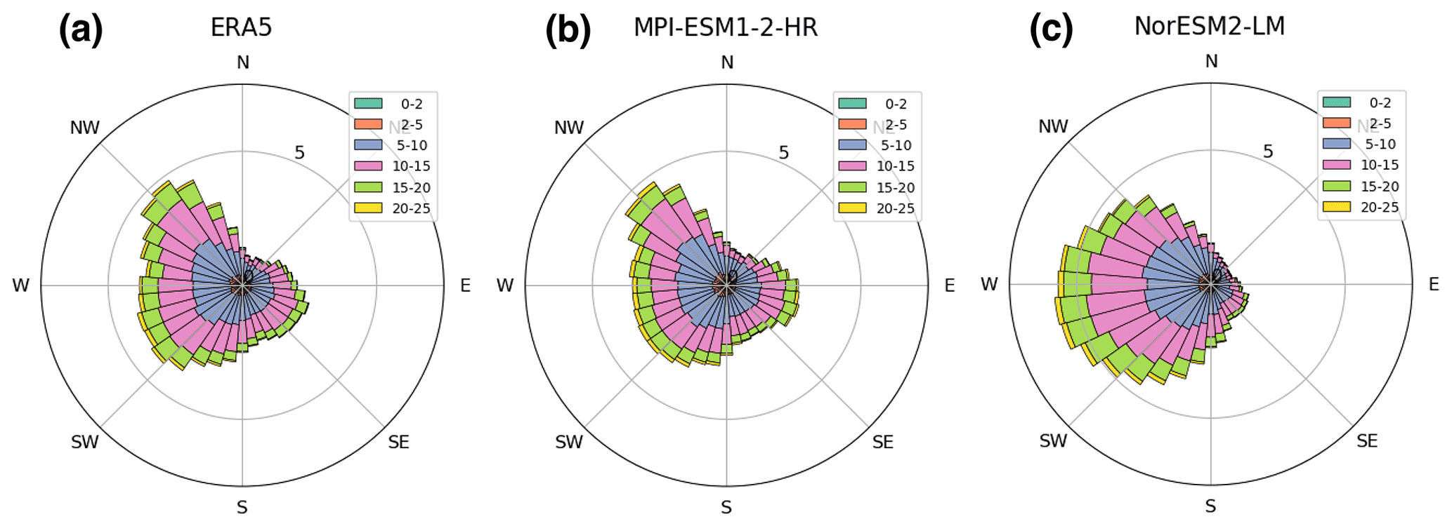
Figure 4Wind roses of the wind climatology at 100 m a.g.l. in the (a) ERA5 reanalysis and simulated by the (b) MPI-ESM1-2-HR and (c) NorESM2-LM CMIP6 models during the historical period (1980–2014) at the Energy Island location. Wind speed bins are in metres per second.
Figure 5 shows the annual cycle of the monthly mean wind speed at 100 m a.g.l. from the CMIP6 models compared to the three reanalyses for the historical period at the Energy Island. The monthly means of nearly all models are primarily within one standard deviation of the monthly mean of the ERA5 reanalysis (blue-shaded area). The three CMIP6 models that significantly fall outside this region are the same models previously flagged in Fig. 3: the two MIROC and CanESM5 model simulations. While the monthly wind speed evolution simulated by these three models follows the phase and amplitude of the reanalysis, their monthly mean wind speeds are too low. The monthly mean wind speeds simulated by the CanESM5 are too low only during the summer and autumn but within the variability of the ERA5 monthly means during the rest of the year.
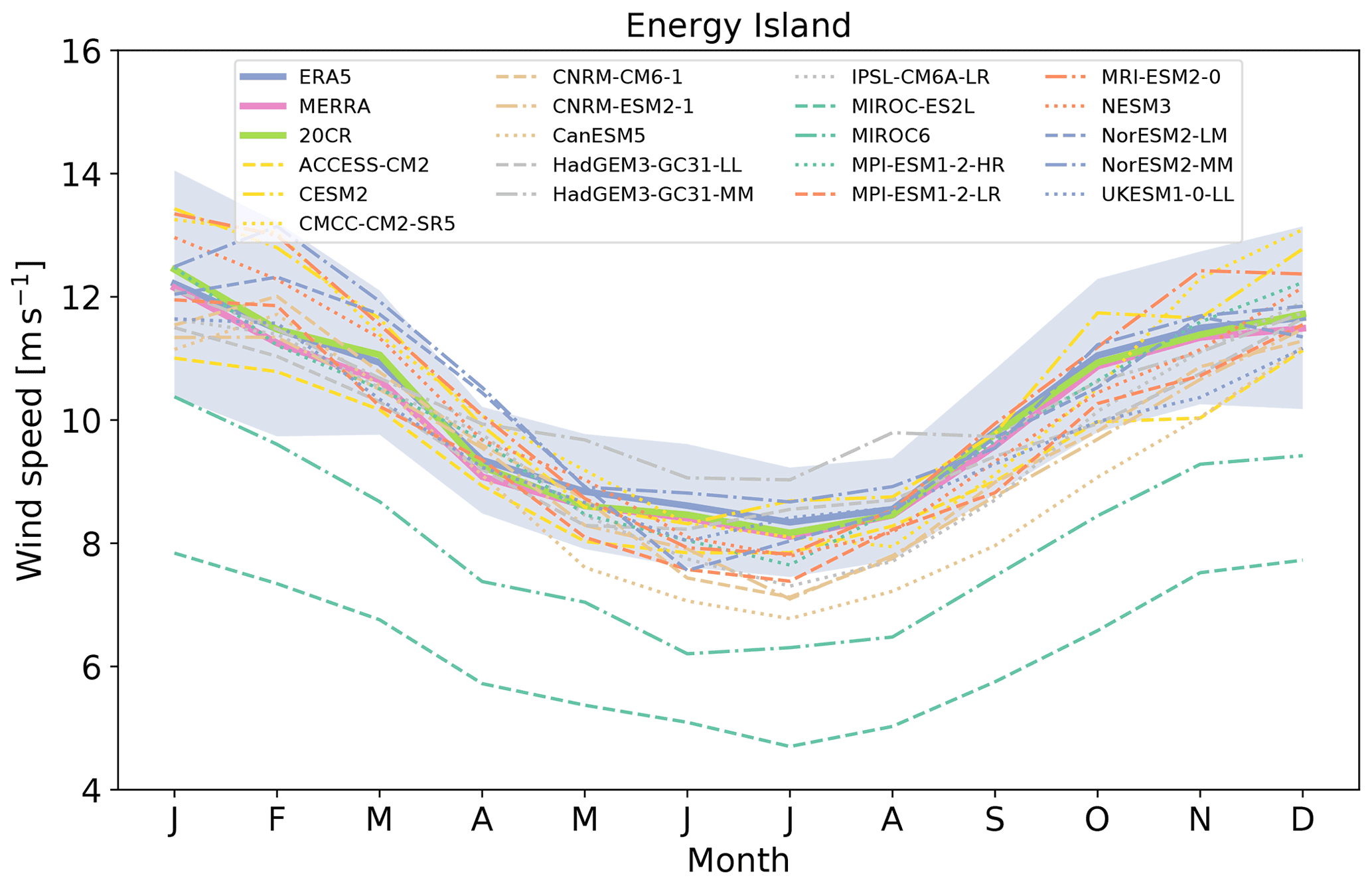
Figure 5The annual cycle of mean monthly wind speed ( and ) at 100 m a.g.l. simulated by the CMIP6 models and that provided by the global reanalyses during the full historical period (1980–2014) for the Energy Island location. The shaded area is the ± 1 standard deviation of the monthly means for the ERA5 reanalysis.
4.2 Evaluation at multiple sites
We carry on with the evaluation of the wind climatology in the CMIP6 models at multiple sites in the North Sea. We use summary heat tables (Fig. 6) to compare the wind climate in the CMIP6 models to that of the ERA5 at 100 m a.g.l., covering the entire historic period, 1980–2014. On average, two-thirds of the models underestimate the mean wind speed when compared to ERA5, especially on the eastern side of the basin (Fig. 6a). At the Ekofisk and IJmuiden sites in the central and southern North Sea, the bias in the mean wind speed compared to ERA5 is more positive; only four CMIP6 model simulations, including those by the MIROC model, overestimate the mean wind speed at Ekofisk. The results are similar among models; when they have small BIAS, they also have small EMD, CEMD, and annual cycle RMSD and vice versa. The only anomaly is the NorESM2-LM model, which has reasonable BIAS, EMD, and RMSD but large deviations in the wind rose as diagnosed by the CEMD (Fig. 6c). These statistics do not detect a better-simulated wind climatology in the CMIP6 CMs than in the ESMs. However, high spatial resolution seems advantageous for wind direction. For example, the CEMD statistics are 2.6–5.2∘ for the 1.875∘ HadGEM3-GC31-LL model but 2.0–3.9∘ for the 0.833∘ HadGEM3-GC31-LL model simulation. This is also true for the MPI-ESM1-2-HR (CEMD = 1.6–3.7∘) versus MPI-ESM1-2-LR (CEMD = 3.9–5.6∘). Based on all four metrics, the simulation using the HadGEM3-GC31-MM model is as good as that using the other two reanalyses. Fernandez-Granja et al. (2021) reached similar conclusions regarding the improvement of the atmospheric circulation in the CMIP6 models.
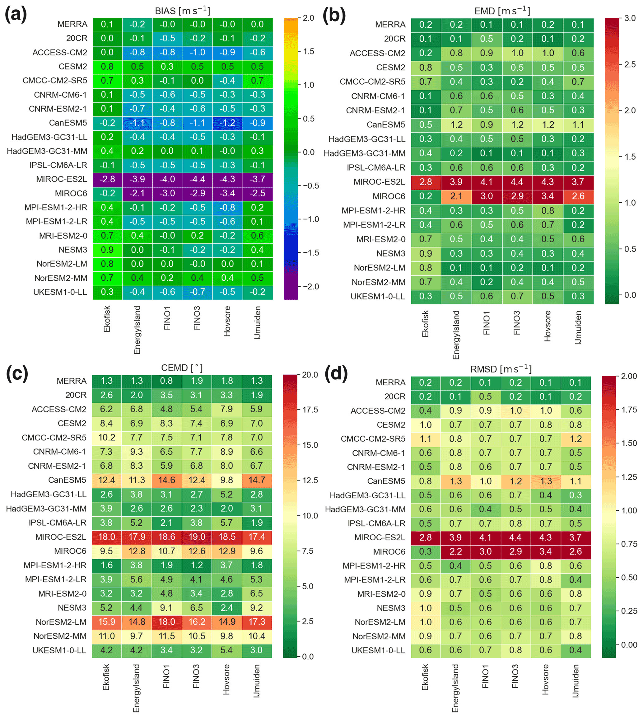
Figure 6Evaluation metrics of the 100 m wind climatologies for the reanalysis and CMIP6 models, i.e. (a) BIAS (m s−1), (b) EMD (m s−1) for the simulated wind speed, (c) CEMD (∘) for simulated wind direction, and (d) RMSD of the mean annual cycle (m s−1), at the six locations in the North Sea for the full historical period (1980–2014). The wind climatologies are evaluated against that of the ERA5.
4.3 Annual energy production at the Energy Island cluster
As described in Sect. 3.3, we perform annual energy production (AEP) calculations for the hypothetical wind farm cluster at the Energy Island. Figure 7 compares the net AEP from the wind farm cluster computed from the wind climate of the reanalysis and the CMIP6 models during the entire historical period 1980–2014. The net AEP values from the MIROC models are nearly half of the other models and are not included in the figure. The mean net AEP for the Energy Island wind farm cluster calculated using the reanalyses is between 56 and 57 TWh. The use of 6-hourly data does not dramatically influence the calculation; if one uses hourly or 3-hourly data in the ERA5 time series, the net AEP is nearly identical and only 0.03 % larger than using the 6-hourly time series, respectively. The wind farm cluster comprises 670 total 15 MW wind turbines; thus, the capacity factor is about 0.64 when using the ERA5 data. The capacity factor estimate is slightly more optimistic than that from COWI for three of the wind farms in the Energy Island cluster, which is about 0.59 (5200 GWh per wind farm according to COWI, 2020).

Figure 7Net annual energy production of the Energy Island wind farm cluster calculated from the time series of the three reanalyses and the CMIP6 models (excluding the MIROC models) for the full historical period (1980–2014).
The net AEP derived from the CMIP6 models is, on average, 4.9 % lower than that computed from the ERA5 data. Only three of the CMIP6 models have positive biases, and the ratio of the net AEP from CMIP6 and that calculated from the ERA5 time series varies between −10 % and 2.4 %. The AEP computed from the HadGEM3-GC31-MM model is 0.27 % of that calculated using the ERA5 time series, which is not surprising since the wind climatology of this model is so close to that of the ERA5 (Fig. 6). The results of the net AEP comparison are consistent with the validation of the wind speed climatology in Fig. 2. The IQR of the net AEP from the CMIP6 is comparable to that from the reanalyses. Considering the nature of the CMIP6 models, these discrepancies are considered well within the expected uncertainty.
Based on the verification statistics presented, we focus on the future changes in the wind climatology using 16 of the 18 models in Table 1. The two CMIP6 simulations using the MIROC models are considered too low compared to the observed historical climatology in the North Sea and excluded from the analysis of the future wind resources.
We assess the changes in wind resources by first examining the large-scale changes in wind speed and wind power density over the whole northern Europe region. We consider two periods of 20 years each: the “past” from 1995 to 2014 and the “future” from 2031 to 2050. Then we examine the wind speed trends in the North Sea by considering the entire 70-year period from 1980 to 2050. We finalize by evaluating the changes in wind speed and power density in the North Sea box and energy production at the Energy Island wind farm cluster from the past to the future.
5.1 Large-scale changes
The spatial distribution of the median relative changes in wind speed and wind power density is shown in Fig. 8. The figures are constructed in the following manner. The annual or seasonal mean wind speed and wind power density of each CMIP6 model are bi-linearly interpolated to a 2.5∘ × 2.5∘ regular grid. We then compute the difference between the means of the periods (2031–2050) and (1995–2014) for each model. We can find the model distribution of the changes for each grid point, and the median is then displayed. The spread of the distributions is used to assess the agreement among the 16 CMIP6 models. Areas without dotted marks represent a significant agreement between the signal (the sign of change) of the models. This way of displaying agreement among the ensemble of models is a standard practice in IPCC assessment reports (IPCC, 2022, 2021). The maps are also made for summer and winter separately. The median of the annual changes at 100 m a.g.l. are primarily negative, minor (1 %–2 % in wind speed, 2 %–4 % in wind power density), and spread in patchy areas where the models disagree on the sign of the changes. During summer, however, median 100 m a.g.l. wind speeds are reduced in the future by 3 %–5 % in a spatially broad area covering the southern North Sea, the British Isles and northern Germany. Similar patterns but larger relative values are seen in the wind power density, with 5 %–15 % reductions. In winter, the Baltic Sea experiences small but regionally consistent increases in wind speed (1 %–3 %) and power density (2 %–8 %) in the future, which are of the same sign in 12 or more models.
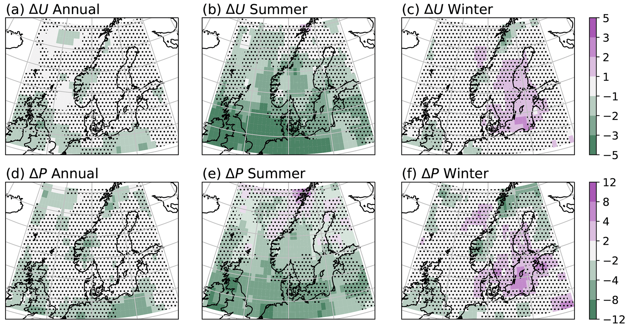
Figure 8Median of the ensemble relative change (%) in 100 m a.g.l. wind speed among the CMIP6 models (a)–(c) and wind power density (d)–(f) between the future (2031–2050) and the past (1995–2014). Medians are computed for the annual means ((a) and (d)), JJA means (summer, (b) and (e)), and DJF means (winter, (c) and (f)). The dotted areas represent areas where less than 75 % (or 12 of 16) of models agree on the sign of the change. See the text for the procedure used to compute the data displayed.
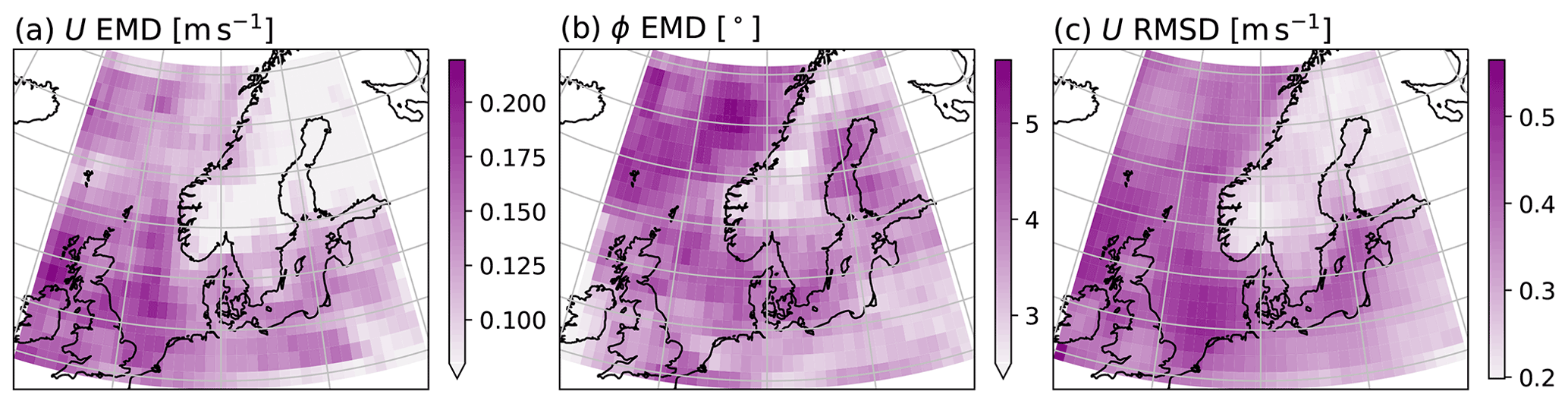
Figure 9Median of the ensemble of (a) EMD of the 100 m a.g.l. wind speed (m s−1), (b) CEMD of the 100 m a.g.l. wind direction (∘]), and (c) RMSD of the annual cycle (m s−1) between the past (1995–2014) and future (2031–2050) in the various CMIP6 models.
Figure 9 shows the maps of the median EMD, CEMD, and RMSD of the annual cycle between the past and future periods. It is interesting to see the most significant changes in EMD concentrating in the middle of the North Sea and East of Scotland, with the lowest values over the Scandinavian peninsula. The median of the CEMD map (Fig. 9b) shows changes in the wind direction distribution with larger values in the north Atlantic off the Norwegian coast. These changes in wind direction could be relevant to wind farm calculations, as will be demonstrated in the next section for the future Energy Island wind farm. The monthly mean RMSD shows the changes in the annual cycle of the monthly mean wind. Figure 9 shows larger values over water than land, especially in the North Sea. This region and that over the southern Baltic Sea agree with the assessment that seasonal changes in wind resources might be significant in this area.
5.2 Wind speed trends
Figure 10 shows the time series of annual mean wind speed averaged over the North Sea box delimited in the map in Fig. 1a. The thin background lines show each CMIP6 model (except for the MIROC models), and the coloured lines show the values for the reanalyses in the historical period. The annual mean wind speed in the reanalyses shows significant variations from year to year, with a standard deviation of 0.33 m s−1, with the lowest value of the annual mean wind speed in 2010 of 9.3 m s−1 and the largest in 1990 of 10.8 m s−1 according to the ERA5 reanalysis.

Figure 10Annual mean wind speed at 100 m a.g.l. using (a) model level winds and (b) a power law relationship (Eq. 4) averaged over the box in Fig. 1a in the CMIP6 models. Also shown are the annual mean of the three reanalyses (colours), the median of all CMIP6 models, and the 5-year rolling mean of the median.
The mean wind speed time series for the CMIP6 models also show significant interannual variations. The median of the CMIP6 models for the historical period lies within the envelope observed by the reanalyses, with a slight overestimation. When looking at the full 70-year record (1980–2050), the median of the CMIP6 models shows slow decadal variations with a trend of −0.032 m s−1 per decade, equivalent to −0.32 % per decade. When examining the models individually, 3 of the 16 CMIP6 models show increases of 0.1 % per decade or more, while 12 show decreases of −0.1 % per decade or more. However, only 5 of the 15 models show significant downward trends with a 99 % significance level based on a Wald test with the Student t distribution.
Several previous studies have used the 10 m a.g.l. wind output to estimate the 100 m a.g.l. wind speed using the power law (Eq. 4), sometimes with a different shear exponent α over the oceans. If used with , the time series of annual mean wind speed look like those in Fig. 10b; such a relation highly overestimates the turbine-height wind speed over water. While the mean in the reanalyses is 10 m s−1, that of the power-law-derived winds during the historical period is 11.4 m s−1, or 12 % larger. In addition, the power-law extrapolated wind speeds exaggerate the trends in wind speed. In the extrapolated winds, the trend in wind speed during 1980–2050 is −0.41 m s−1 per decade, 28 % larger than that obtained by using the model-computed 100 m winds. Additionally, the significance level of the trends is enhanced, with now 8 of the 16 models having significant downward trends (with a 99 % significance level based on a Wald test) in wind speed.
5.3 Inter-model spread and annual cycle
The changes between the past (1995–2014) and the future (2031–2050) in mean wind speed and wind power density in the CMIP6 models for the North Sea box (Fig. 1) are detailed in Fig. 11. We show the changes for the annual mean and four seasons: DJF (winter; December–February), MAM (spring; March–May), JJA (summer; June–August) and SON (autumn, September–November). Changes in annual mean wind speed have a slight negative median and large spread. Only 3 of the 16 CMIP6 models have changes that are significant at the 95 % level (Fig. A1). Similar conclusions, but with an even larger spread, can be drawn for the changes in annual mean power density that vary from −10 % to 8 %. Using the CMIP model-derived air density instead of standard atmosphere values does not significantly alter the annual mean wind power density results. However, it still narrows down the range of the relative differences.
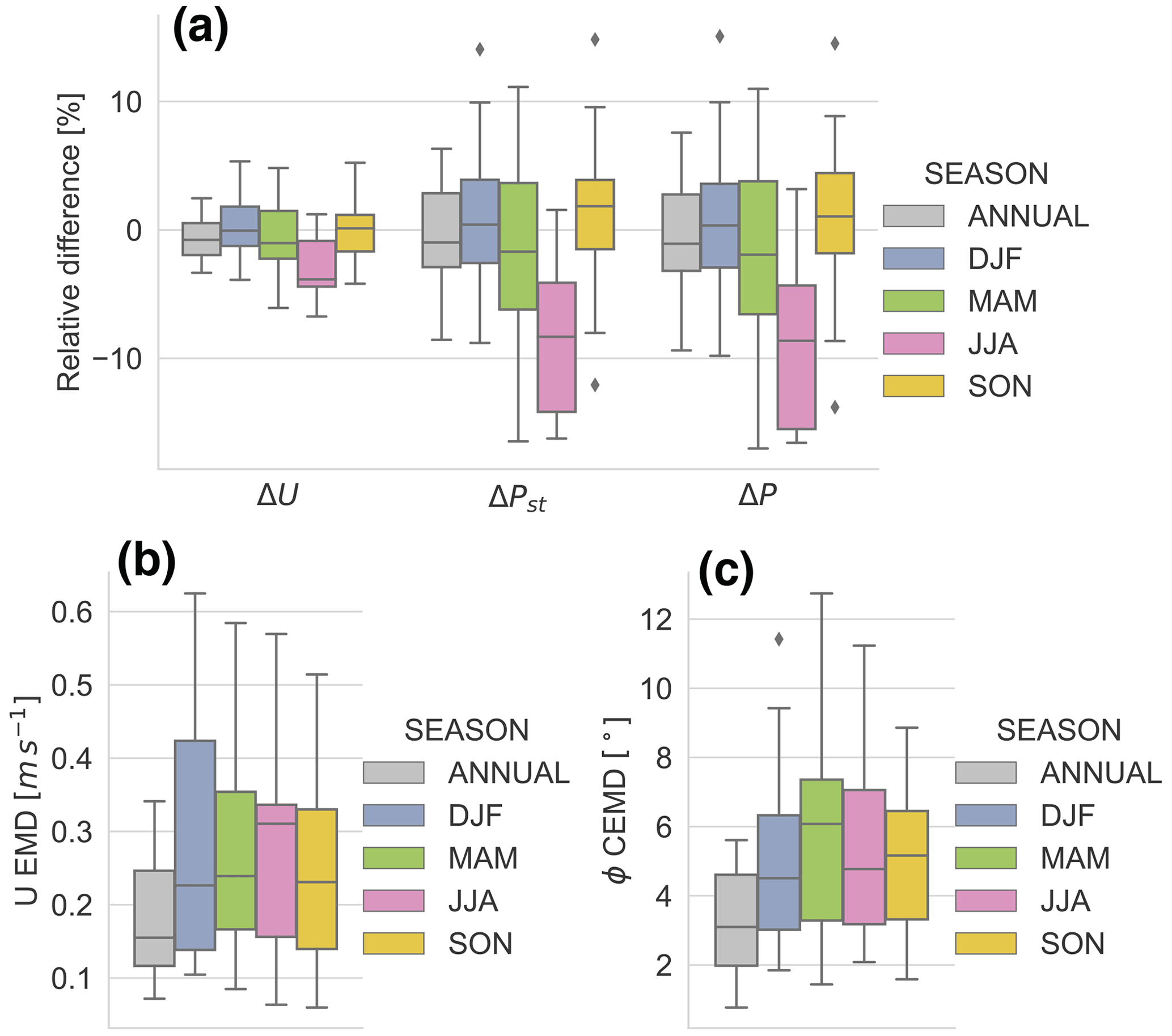
Figure 11(a) Boxplot of the relative mean changes between the past (1995–2014) and the future (2031–2050) averaged over the North Sea box in Fig. 1a in 100 m a.g.l. wind speed (ΔU), standard wind power density (ΔPST), and wind power density (ΔP). Boxplot of the changes in distribution between the past (1995–2014) and the future (2031–2050) as (b) wind speed EMD and (c) wind direction CEMD. The boxes show the spread among the 16 CMIP6 models (excluding MIROC).
The results are different when values are averaged over separate seasons. The decrease in the JJA mean wind speed is significant in half the models, with a range of 4 %–6 % (or 0.4–0.6 m s−1). Many models also have significant changes in power density during the summer, with maximum decreases on the order of 15 %. Only one model has a positive increase in summer wind speed and power density over the North Sea. The changes in surface air density are nearly significant for all models but of no consistent sign among the models. Since changes in temperature due to climate change are significant in this region (IPCC, 2021), surface pressure must also play a significant role. However, their impact on the wind power density is mostly not significant.
Figure 11b shows the EMD calculated between the past (1995–2014) and future (2031–2050) wind speed distributions in the 16 selected CMIP6 models. Changes in EMD vary between 0.07–0.34 m s−1, which is comparable to the values in the historical period when compared to the atmospheric reanalyses (Fig. 5). Larger EMD values are seen for all seasons, especially in summer. The spread among ensemble members is also much larger for the individual seasons, particularly in winter; however, this is partly an artefact of the reduced sample size. The wind direction CEMD between the past and the future is shown in Fig. 11c. The wind direction CEMD is between 0.5 and 5.6∘ in the annual wind distributions, with a median of 3∘. The wind direction CEMD is larger for the individual seasons, especially during the spring (median of 6∘), when the spread is also the largest.
We calculate the energy production of the wind farm cluster on the proposed Energy Island. The changes in EP (reference, standard, and net) between the past (1995–2014) and the future (2031–2050) are presented as boxplots in Fig. 12 for the whole year and the four individual seasons. The median reference AEP of the wind farm cluster is expected to decrease by about −1.3 %, as anticipated by the changes in wind speed. When we consider wakes, the median decrease in AEP is −1.5 %, and when we consider wakes and changes in air density, the median decline is −1.9 %. The spread among the CMIP6 models is large (with an IQR of 2.9 %–3.6 %) and increases from the reference value when wakes and density changes are considered. The capacity factor of the wind farm cluster averaged over all CMIP6 models is reduced from 57.6 % in the past to 56.8 % in the future.
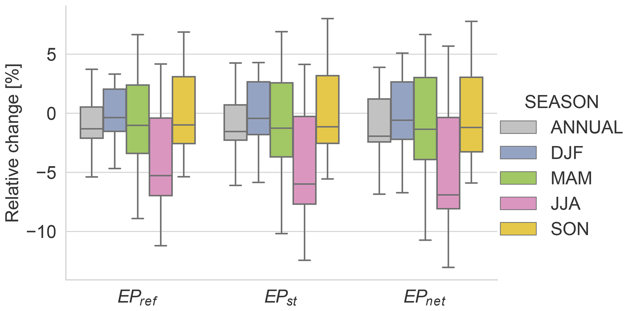
Figure 12Boxplot of the change in energy production of the future Energy Island wind farm complex considering reference EP (no wake losses), standard EP (standard air density), and net EP (including wake losses and air density). The changes are computed between the past (1995–2014) and the future (2031–2050) in the various CMIP6 models (excluding MIROC).
According to the changes in seasonal net EP between the past and the future, the median of all CMIP6 models is expected to decrease in all seasons but very little in winter (−0.6 %) and markedly more in the summer (−6.9 %). The IQR of the changes in net EP also increases from winter (4.9 %) to summer (7.7 %). Similar trends in the capacity factors are calculated using the net seasonal EP (not shown).
In all the energy production estimates, the median change in EPref is decreased by including the wake losses. Including the effect of the changes in air density further reduces the energy production in the future in most models. For example, the summer energy production is predicted to change by −5.3 %, in the reference calculation, and −6.0 %, and −6.9 %, when wake losses and air density changes are considered, respectively. The effect of the decreases in the overall energy production (in the denominator) is not a primary factor. In the annual mean, median energy production is expected to decrease by −18 GW when no wakes are considered but −25 and −33 GW when wakes and air density changes in the future are considered, respectively.
We show that most CMIP6 models can represent the hub-height wind climatology of the historical period in the North Sea well, especially considering the large model grid spacing. When using the 1980–2014 time series of wind speed and wind direction and a hypothetical wind farm cluster, AEP calculations are within 10 % of that estimated using the wind time series extracted from reanalyses data for the same period. The wind climate of the CMIP6 models is similar to that observed in this region in terms of wind speed and wind direction. The CMIP6 simulation using the HadGEM3-GC31-MM model is as good quality as any of the reanalyses in terms of representing the wind climate of the North Sea in the historical period.
Over the North Sea, we demonstrate that using the 10 m wind speed output from CMIP6 models with the power law with overestimates the 100 m mean wind speed over the sea by 20 %–30 %. This extrapolation will accordingly also exaggerate trends in wind speed and their significance. The wind shear in the boundary layer over the sea is generally smaller than that over the land (Peña and Hahmann, 2012; Hahmann et al., 2015) because of the low surface roughness length. But because the wind shear also depends on atmospheric stability, which could change, e.g. as the surface warms, the power law with a constant shear exponent becomes even less accurate for determining turbine-height winds (Badger et al., 2016). Over land, the wind shear exponent in the boundary layer is very variable (with typical values of α=0.16 over grass to α=0.28 over forest) and depends on the heights chosen, surface roughness length, and atmospheric stability (Emeis, 2018). Over non-homogeneous terrain, the wind shear and power law exponent at a site are also directional quantities, imprinting in the wind profile at various heights of the upstream flow at varying distances.
The changes in wind resources in northern Europe shown here are somewhat inconsistent with some of those provided by the CMIP5 and Euro-CORDEX data in previous studies. Using ensembles of CMIP5 model output of various compositions and sizes, studies generally show an increase in wind speed in central and northern Europe and decreases in southern Europe (Reyers et al., 2016; Carvalho et al., 2017; Gonzalez et al., 2019; Karnauskas et al., 2018; Devis et al., 2018). This is consistent with the projected northward shift and eastward extension of the North Atlantic jet and storm track into Europe under climate change (Zappa et al., 2015). Studies using Euro-CORDEX data, however, have more varied results. Tobin et al. (2016) used an ensemble of nine Euro-CORDEX models and showed that changes in the AEP of the future European wind farms would remain within ±5 % across the 21st century. Moemken et al. (2018) used a different set of nine Euro-CORDEX models, which projected small changes in mean annual and winter power output for large parts of Europe in future decades, but a considerable decrease for summer. The two Euro-CORDEX studies used different treatments of the wind speeds (one extrapolation from 10 m, the other interpolation and bias correction). They used models that do not account for changes in land use included in the global climate model forcing their regional climate model simulations.
Carvalho et al. (2021) used 10 m wind extrapolation using ERA5-derived shear parameter of a large ensemble of CMIP6 models (including the ones used in this study) and concluded that future energy resources are expected to decline by 10 %–20 % in practically all of Europe. The study also remarks that this contrasts with CMIP5 studies, which show an increase in northern Europe. The analysis of the 850 hPa zonal wind in Oudar et al. (2020) also finds differences in response between CMIP5 and CMIP6 simulations in the position of the jets in the North Atlantic and western Europe region. Additionally, Gonzalez et al. (2019) isolated the components associated with “large-scale” atmospheric circulation changes in the CMIP5 simulations and found that likely two processes are responsible. The first is related to changes in the large-scale atmospheric circulation, while the second is likely more local connected to changes in the near-surface boundary layer. This conclusion further emphasizes our hypothesis that the 10 m wind extrapolation with constant shear is likely to miss some of the processes controlling the future changes in wind resources.
We use the layout and turbine characteristics of a hypothetical massive wind farm cluster in the North Sea to evaluate future changes in wind speed and wind direction distributions for energy production in this region. Our results show that the summer decreases in wind speed are amplified when converted to energy production and further strengthened when we include the inter-turbine wakes and changes in air density. This is because changes in wind speed impact power production in different ways depending on the wind speed. A change in wind speed near the cut in (usually 3–5 m s−1) of a power curve will change the energy production, while the same decrease in the rated power section of the power curve will not. Therefore, changes in wind speed at lower wind speeds are amplified when considering energy production. The difference in energy production is thus sensitive to the power curve of the chosen turbine type. Devis et al. (2018) showed that the projected wind power changes might vary by up to half their magnitude, depending on the turbine type and region of interest. In addition, since the wake of one wind turbine decreases the wind speed downstream, including wake effects can reduce the wind speed near the cut in and further amplify the wind farm's response to wind speed changes. Because the wind direction distribution at a site dictates the combined magnitude and direction of the turbine wakes, it is expected that changes in wind direction in the future could also influence the efficiency of future wind farms, especially if the wind farm layout is optimized for present wind conditions.
In the calculation of the energy production of the Energy Island wind farm cluster, the engineering model does not consider the influence of the wind farm on the large-scale atmospheric flow (e.g. Nygaard, 2014; Fischereit et al., 2022). Large wind farms and clusters of wind farms can further decrease the wind farm efficiency by 10 %–30 % in offshore regions with moderate wind speeds and relatively wide turbine spacing (Volker et al., 2017) depending on the size of the wind farm. This aspect further impacts the response of a given wind farm cluster to future changes in the wind climate and should be considered in future studies.
This study examines the future mid-century changes in hub-height wind speed and hub-height power density over northern Europe using an ensemble of CMIP6 model output according to the historical and SSP5-8.5 scenario simulations. We found non-significant differences between the past (1995–2014) and the future (2031–2050) in the annual mean of these quantities. However, over 75 % of the models agree on the decrease in the resources during the summer in the North Sea. In the Baltic Sea, over 75 % of the models agree on an increase in wind resources during winter. However, for these future predictions to be meaningful, including as many models as possible is vital because models often disagree, and randomly selecting models might produce very different results.
The large-scale characteristics of the wind resources in the North Sea at levels accessible to present wind turbines are well represented by current reanalysis compared to long-term tall mast measurements. The CMIP6 models run for the historical period can also capture the main features of the wind resources in this region. The errors in mean wind speed in a few CMIP6 models run at relatively high resolution lie within the spread of the three reanalyses.
Extrapolating wind speeds from 10 m to turbine height using a constant power law is a poor approximation in many circumstances and will often exaggerate future changes in wind resources. This is relevant because the variables that control the value of the power law exponent (i.e. surface roughness length linked to vegetation changes and atmospheric stability) are likely to change in the future.
The changes in wind energy production shown here are in the range of 5 %–10 %. They would most likely be considered inconsequential, especially because energy systems, including large wind farms, are often over-designed to guarantee the delivery of electricity under all conditions. However, such changes represent a sizeable economic impact in the form of higher financing prices and revenue loss by the wind farm operator. Regarding the design of the future low-emission power system, it is convenient that the significant decrease in wind resources occurs during summer when the wind electricity shortfall can be replaced by solar-generated electricity. Still, the consequences of reduced resources and possible changes in variability to the power system operation are more complex and not included in this study. As with the example provided here, power system studies must also use the complete chain of models and consider the effect of simplifications and the model numerical imprint on the model-generated time series.
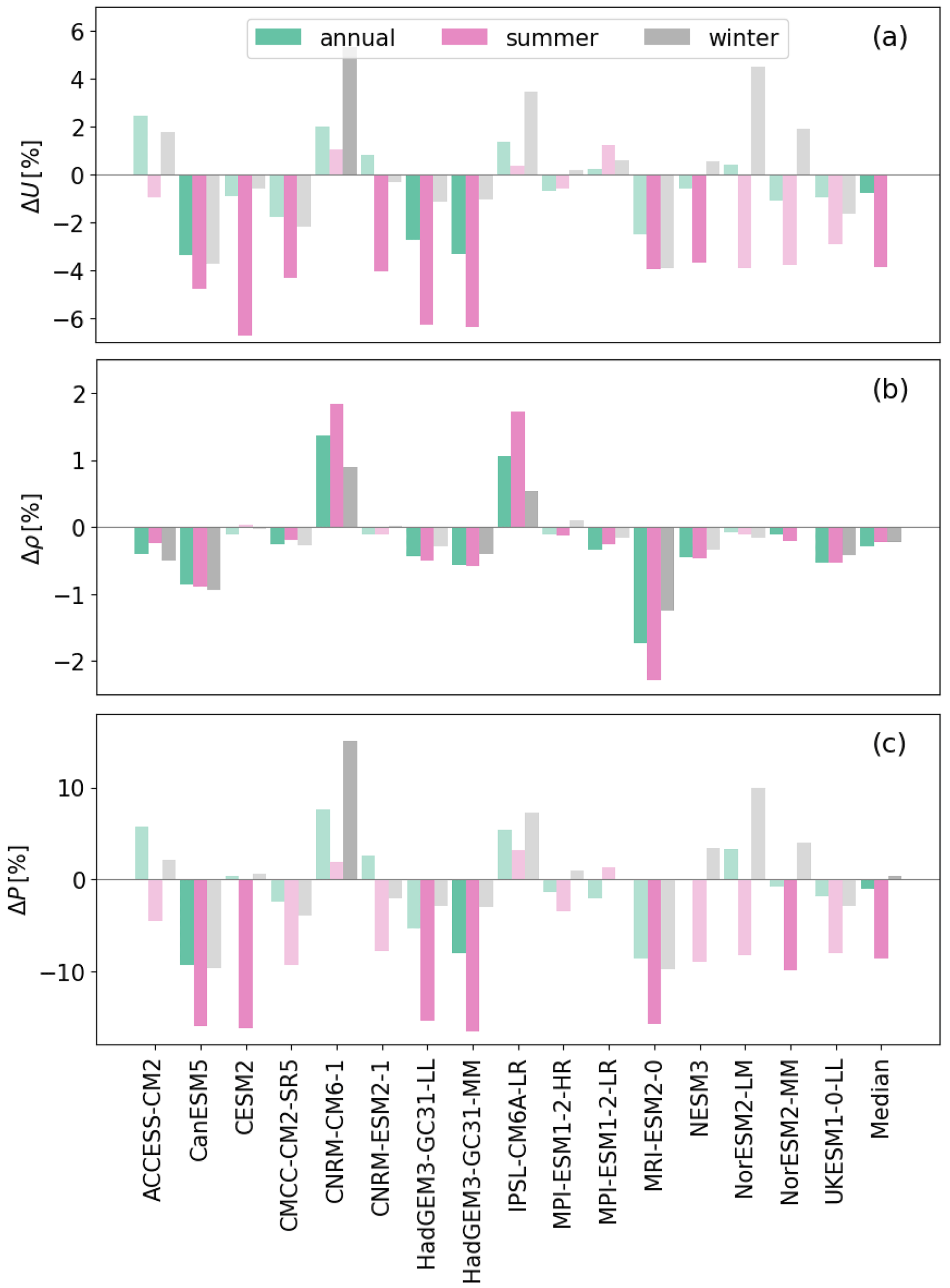
Figure A1Relative changes in (a) wind speed, (b) surface air density, and (c) wind power density between the future and the past averaged over the North Sea box. Light coloured bars are not significant at the 95 % level.
We provide examples of the Python code used to search, extract, interpolate, and locally write the winds in the CMIP6 data. The code, named future-wind, can be found at https://doi.org/10.5281/zenodo.7260128 (Hahmann, 2022). The wake calculations were performed using PyWake, available at https://github.com/DTUWindEnergy/PyWake (last access: 15 November 2022) (DOI: https://doi.org/10.5281/zenodo.2562662, Pedersen et al., 2019).
The NEWA data are available from https://doi.org/10.11583/DTU.14414096.v1 (Hahmann et al., 2021). The ERA5 data were downloaded from the ECMWF at the Copernicus Climate Change Service (C3S) Climate Data Store (CDS), at https://doi.org/10.24381/cds.adbb2d47 (Hersbach et al., 2018). The MERRA2 data are downloaded from the Distributed Active Archive Center (GSFC DAAC) at https://doi.org/10.5067/VJAFPLI1CSIV (GMAO, 2015). The NOAA/CIRES/DOE 20th Century Reanalysis (V3) data were provided by the NOAA PSL, Boulder, Colorado, USA, from their website at https://psl.noaa.gov/data/gridded/data.20thC_ReanV3.html (NOAA, 2019).
ANH wrote the first draft, extracted the CMIP6 data, and analysed the results. OGS carried out the wind farm calculations. ANH, OGS, and AP participated in the analysis design and the manuscript's writing and editing.
At least one of the (co-)authors is a member of the editorial board of Wind Energy Science. The peer-review process was guided by an independent editor, and the authors also have no other competing interests to declare.
Publisher's note: Copernicus Publications remains neutral with regard to jurisdictional claims in published maps and institutional affiliations.
The following people and organizations have kindly provided the tall mast data used for the verification. FINO 1, 2, and 3 were supplied by the German Federal Maritime And Hydrographic Agency (BSH). Ijmuiden data from the Meteorological Mast Ijmuiden were provided by the Energy Research Center of the Netherlands (ECN) and processed by Peter Kalverla from Wageningen University. Birgitte Rugaard Furevik at the Geophysics Institute, University of Bergen, kindly supplied the Ekofisk data. Høvsøre data were provided by the Technical University of Denmark (DTU). Support for the 20th Century Reanalysis Project version 3 dataset is provided by the US Department of Energy, Office of Science, Biological and Environmental Research (BER); the National Oceanic and Atmospheric Administration Climate Program Office; and the NOAA Physical Sciences Laboratory. The CMIP6 multi-model ensemble data were downloaded through the distributed data archive developed and operated by the Earth System Grid Federation (ESGF; https://esgf.llnl.gov/, last access: 13 November 2022).
The authors thank Sarah Pryor and Jake Badger for the many fruitful discussions. Graziela Luzia created the prototype data download script.
Andrea N. Hahmann and Alfredo Peña acknowledge the support of the Danish Ministry of Foreign Affairs, administered by the Danida Fellowship Centre under the project “Multi-scale and Model-scale Evaluation of Wind Atlases” (MEWA). Oscar García-Santiago was funded by the European Union Horizon 2020 research and innovation programme under grant agreement no. 861291 as part of the Train2Wind Marie Skłodowska-Curie ITN (https://www.train2wind.eu/, last access: 13 November 2022).
This paper was edited by Amy Robertson and reviewed by Nicola Bodini and one anonymous referee.
Alonso Díaz, Y., Bezanilla, A., Roque, A., Centella, A., Borrajero, I., and Martinez, Y.: Wind resource assessment of Cuba in future climate scenarios, Wind Eng., 43, 311–326, https://doi.org/10.1177/0309524X18780399, 2019. a
Badger, M., Peña, A., Hahmann, A. N., Mouche, A. A., and Hasager, C. B.: Extrapolating satellite winds to turbine operating heights, J. Appl. Meteorol. Clim., 55, 975–991, https://doi.org/10.1175/JAMC-D-15-0197.1, 2016. a
Barthelmie, R. J. and Jensen, L. E.: Evaluation of wind farm efficiency and wind turbine wakes at the Nysted offshore wind farm, Wind Energy, 13, 573–586, https://doi.org/10.1002/we.408, 2010. a
Beiter, P., Cooperman, A., Lantz, E., Stehly, T., Shields, M., Wiser, R., Telsnig, T., Kitzing, L., Berkhout, V., and Kikuchi, Y.: Wind power costs driven by innovation and experience with further reductions on the horizon, Wiley Interdiscip. Rev. Energy Environ., 10, e398, https://doi.org/10.1002/wene.398, 2021. a
Boucher, O., Servonnat, J., Albright, A. L., Aumont, O., Balkanski, Y., Bastrikov, V., Bekki, S., Bonnet, R., Bony, S., Bopp, L., Braconnot, P., Brockmann, P., Cadule, P., Caubel, A., Cheruy, F., Codron, F., Cozic, A., Cugnet, D., D'Andrea, F., Davini, P., de Lavergne, C., Denvil, S., Deshayes, J., Devilliers, M., Ducharne, A., Dufresne, J.-L., Dupont, E., Éthé, C., Fairhead, L., Falletti, L., Flavoni, S., Foujols, M.-A., Gardoll, S., Gastineau, G., Ghattas, J., Grandpeix, J.-Y., Guenet, B., Guez, Lionel, E., Guilyardi, E., Guimberteau, M., Hauglustaine, D., Hourdin, F., Idelkadi, A., Joussaume, S., Kageyama, M., Khodri, M., Krinner, G., Lebas, N., Levavasseur, G., Lévy, C., Li, L., Lott, F., Lurton, T., Luyssaert, S., Madec, G., Madeleine, J.-B., Maignan, F., Marchand, M., Marti, O., Mellul, L., Meurdesoif, Y., Mignot, J., Musat, I., Ottlé, C., Peylin, P., Planton, Y., Polcher, J., Rio, C., Rochetin, N., Rousset, C., Sepulchre, P., Sima, A., Swingedouw, D., Thiéblemont, R., Traore, A. K., Vancoppenolle, M., Vial, J., Vialard, J., Viovy, N., and Vuichard, N.: Presentation and Evaluation of the IPSL-CM6A-LR Climate Model, J. Adv. Model. Earth Sy., 12, e2019MS002010, https://doi.org/10.1029/2019MS002010, 2020. a
Carvalho, D., Rocha, A., Gomez-Gesteira, M., and Santos, C. S.: Potential impacts of climate change on European wind energy resource under the CMIP5 future climate projections, Renew. Energ., 101, 29–40, https://doi.org/10.1016/j.renene.2016.08.036, 2017. a
Carvalho, D., Rocha, A., Costoya, X., DeCastro, M., and Gómez-Gesteira, M.: Wind energy resource over Europe under CMIP6 future climate projections: What changes from CMIP5 to CMIP6, J. Renew. Sust. Energ., 151, 111594, https://doi.org/10.1016/j.rser.2021.111594, 2021. a
Chang, T.-J., Chen, C.-L., Tu, Y.-L., Yeh, H.-T., and Wu, Y.-T.: Evaluation of the climate change impact on wind resources in Taiwan Strait, Energy Convers. Manag., 95, 435–445, https://doi.org/10.1016/j.enconman.2015.02.033, 2015. a
Chen, L.: Impacts of climate change on wind resources over North America based on NA-CORDEX, Renew. Energ., 153, 1428–1438, https://doi.org/10.1016/j.renene.2020.02.090, 2020. a, b
Cherchi, A., Fogli, P. G., Lovato, T., Peano, D., Iovino, D., Gualdi, S., Masina, S., Scoccimarro, E., Materia, S., Bellucci, A., and Navarra, A.: Global Mean Climate and Main Patterns of Variability in the CMCC-CM2 Coupled Model, J. Adv. Model. Earth Sy., 11, 185–209, https://doi.org/10.1029/2018MS001369, 2019. a
Cinquini, L., Crichton, D., Mattmann, C., Harney, J., Shipman, G., Wang, F., Ananthakrishnan, R., Miller, N., Denvil, S., Morgan, M., Pobre, Z., Bell, G. M., Doutriaux, C., Drach, R., Williams, D., Kershaw, P., Pascoe, S., Gonzalez, E., Fiore, S., and Schweitzer, R.: The Earth System Grid Federation: An open infrastructure for access to distributed geospatial data, Futur. Gener. Comput. Syst., 36, 400–417, https://doi.org/10.1016/j.future.2013.07.002, 2014. a
COWI: Vindressource, layouts og energiproduktion For Bornholm I + II, Nordsøen II + III Og Området Vest For Nordsøen II + III, Tech. rep., Danish Energy Agency, https://ens.dk/sites/ens.dk/files/Vindenergi/2-3_vindressource_layouts_og_energiproduktion.pdf (last access: 13 November 2022), 2020. a, b, c, d
Cronin, J., Anandarajah, G., and Dessens, O.: Climate change impacts on the energy system: a review of trends and gaps, Climatic Change, 151, 79–93, https://doi.org/10.1007/s10584-018-2265-4, 2018. a
Danabasoglu, G., Lamarque, J.-F., Bacmeister, J., Bailey, D. A., DuVivier, A. K., Edwards, J., Emmons, L. K., Fasullo, J., Garcia, R., Gettelman, A., Hannay, C., Holland, M. M., Large, W. G., Lauritzen, P. H., Lawrence, D. M., Lenaerts, J. T. M., Lindsay, K., Lipscomb, W. H., Mills, M. J., Neale, R., Oleson, K. W., Otto-Bliesner, B., Phillips, A. S., Sacks, W., Tilmes, S., van Kampenhout, L., Vertenstein, M., Bertini, A., Dennis, J., Deser, C., Fischer, C., Fox-Kemper, B., Kay, J. E., Kinnison, D., Kushner, P. J., Larson, V. E., Long, M. C., Mickelson, S., Moore, J. K., Nienhouse, E., Polvani, L., Rasch, P. J., and Strand, W. G.: The Community Earth System Model Version 2 (CESM2), J. Adv. Model. Earth Sy., 12, e2019MS001916, https://doi.org/10.1029/2019MS001916, 2020. a
Devis, A., Van Lipzig, N. P. M., and Demuzere, M.: Should future wind speed changes be taken into account in wind farm development?, Environ. Res. Lett., 13, 64012, https://doi.org/10.1088/1748-9326/aabff7, 2018. a, b, c
Dörenkämper, M., Olsen, B. T., Witha, B., Hahmann, A. N., Davis, N. N., Barcons, J., Ezber, Y., García-Bustamante, E., González-Rouco, J. F., Navarro, J., Sastre-Marugán, M., Sīle, T., Trei, W., Žagar, M., Badger, J., Gottschall, J., Sanz Rodrigo, J., and Mann, J.: The Making of the New European Wind Atlas – Part 2: Production and evaluation, Geosci. Model Dev., 13, 5079–5102, https://doi.org/10.5194/gmd-13-5079-2020, 2020. a, b
Emeis, S.: Wind Energy Meteorology: Atmospheric Physics for Wind Power Generation, second edn., Green Energy and Technology, Springer International Publishing, Cham, ISBN 978-3-319-72858-2, https://doi.org/10.1007/978-3-319-72859-9, 2018. a
ESGF: esgf-pyclient, ESGF [code], https://esgf-pyclient.readthedocs.io/en/latest/, last access: 13 November 2022. a
Eyring, V., Bony, S., Meehl, G. A., Senior, C. A., Stevens, B., Stouffer, R. J., and Taylor, K. E.: Overview of the Coupled Model Intercomparison Project Phase 6 (CMIP6) experimental design and organization, Geosci. Model Dev., 9, 1937–1958, https://doi.org/10.5194/gmd-9-1937-2016, 2016a. a
Eyring, V., Gleckler, P. J., Heinze, C., Stouffer, R. J., Taylor, K. E., Balaji, V., Guilyardi, E., Joussaume, S., Kindermann, S., Lawrence, B. N., Meehl, G. A., Righi, M., and Williams, D. N.: Towards improved and more routine Earth system model evaluation in CMIP, Earth Syst. Dynam., 7, 813–830, https://doi.org/10.5194/esd-7-813-2016, 2016b. a
Fernandez-Granja, J. A., Casanueva, A., Bedia, J., and Fernandez, J.: Improved atmospheric circulation over Europe by the new generation of CMIP6 earth system models, Clim. Dynam., 56, 3527–3540, https://doi.org/10.1007/s00382-021-05652-9, 2021. a
Fischereit, J., Brown, R., Larsén, X. G., Badger, J., and Hawkes, G.: Review of Mesoscale Wind-Farm Parametrizations and Their Applications, Bound.-Lay Meteorol., 182, 175–224, https://doi.org/10.1007/s10546-021-00652-y, 2022. a
Gaertner, E., Rinker, J., Sethuraman, L., Zahle, F., Anderson, B., Barter, G., Abbas, N., Meng, F., Bortolotti, P., Skrzypinski, W., Scott, G., Feil, R., Bredmose, H., Dykes, K., Shields, M., Allen, C., and Viselli, A.: Definition of the IEA 15-Megawatt Offshore Reference Wind, Tech. Rep., National Renewable Energy Laboratory, https://www.nrel.gov/docs/fy20osti/75698.pdf (last access: 13 November 2022), 2020. a
Gelaro, R., McCarty, W., Suarez, M. J., Todling, R., Molod, A., Takacs, L., Randles, C. A., Darmenov, A., Bosilovich, M. G., Reichle, R., Wargan, K., Coy, L., Cullather, R., Draper, C., Akella, S., Buchard, V., Conaty, A., Da Silva, A., Gu, W., Kim, G.-K., Koster, R. D., Lucchesi, R., Merkova, D., Nielsen, J. E., Partyke, G., Pawson, S., Putman, W., Reinecker, M., Schubert, S. D., Sienkiewicz, M., and Zhao, B.: The Modern-Era Retrospective Analysis for Research and Applications, Version 2 (MERRA-2), J. Climate, 30, 5419–5454, https://doi.org/10.1175/JCLI-D-16-0758.1, 2017. a
Gernaat, D. E., de Boer, H. S., Daioglou, V., Yalew, S. G., Müller, C., and van Vuuren, D. P.: Climate change impacts on renewable energy supply, Nat. Clim. Change, 11, 119–125, https://doi.org/10.1038/s41558-020-00949-9, 2021. a, b
Giorgi, F. and Gutowski, W. J.: Regional Dynamical Downscaling and the CORDEX Initiative, Annu. Rev. Environ. Resour., 40, 467–490, 2015. a
Global Modeling and Assimilation Office (GMAO): tavg1_2d_slv_Nx: 2d, 1-Hourly, Time-Averaged, Single-Level, Assimilation, Single-Level Diagnostics V5.12.4, Greenbelt, MD, USA, Goddard Earth Sciences Data and Information Services Center (GES DISC) [data set], https://doi.org/10.5067/VJAFPLI1CSIV, 2015. a
Göçmen, T., van der Laan, P., Réthoré, P.-E., Diaz, A. P., Larsen, G. C., and Ott, S.: Wind turbine wake models developed at the Technical University of Denmark: A review, Renew. Sustain. Energy Rev., 60, 752–769, https://doi.org/10.1016/j.rser.2016.01.113, 2016. a
Gonzalez, P. L., Brayshaw, D. J., and Zappa, G.: The contribution of North Atlantic atmospheric circulation shifts to future wind speed projections for wind power over Europe, Clim. Dynam., 53, 4095–4113, https://doi.org/10.1007/s00382-019-04776-3, 2019. a, b
GWEC: Global Offshore Wind: Annual Market Report 2020, Tech. Rep. February, Global Wind Energy Council, Bru, https://gwec.net/wp-content/uploads/2020/12/GWEC-Global-Offshore-Wind-Report-2020.pdf (last access: 13 November 2022), 2020. a
GWEC: Global Wind Report 2021, Tech. Rep., Global Wind Energy Council, https://gwec.net/wp-content/uploads/2021/03/GWEC-Global-Wind-Report-2021.pdf (last access: 13 November 2022), 2021. a
Hahmann, A. N.: future-wind Initial Release. In Wind Energy Sciences (v0.1.0), Zenodo [code], https://doi.org/10.5281/zenodo.7260128, 2022. a
Hahmann, A. N., Vincent, C. L., Peña, A., Lange, J., and Hasager, C. B.: Wind climate estimation using WRF model output: Method and model sensitivities over the sea, Int. J. Climatol., 35, 3422–3439, 2015. a
Hahmann, A. N., Sīle, T., Witha, B., Davis, N. N., Dörenkämper, M., Ezber, Y., García-Bustamante, E., González-Rouco, J. F., Navarro, J., Olsen, B. T., and Söderberg, S.: The making of the New European Wind Atlas – Part 1: Model sensitivity, Geosci. Model Dev., 13, 5053–5078, https://doi.org/10.5194/gmd-13-5053-2020, 2020. a, b
Hahmann, A. N., Sīle, T., Witha, B., Davis, N., Dörenkämper, N., Ezber, Y., García-Bustamante, E., González-Rouco, J. F., Navarro, J, Olsen, B. T., Söderberg, S., Barcons, J, Sastre-Marugán, M., Trei, W., Žagar, M., Badger, J., Gottschall, J., Sanz Rodrigo, J., Mann, J., and Vasiljevic, N.: New European Wind Atlas: Mesoscale Atlas, Technical University of Denmark [data set], https://doi.org/10.11583/DTU.14414096.v1, 2021. a
Hajima, T., Watanabe, M., Yamamoto, A., Tatebe, H., Noguchi, M. A., Abe, M., Ohgaito, R., Ito, A., Yamazaki, D., Okajima, H., Ito, A., Takata, K., Ogochi, K., Watanabe, S., and Kawamiya, M.: Development of the MIROC-ES2L Earth system model and the evaluation of biogeochemical processes and feedbacks, Geosci. Model Dev., 13, 2197–2244, https://doi.org/10.5194/gmd-13-2197-2020, 2020. a
Hersbach, H., Bell, B., Berrisford, P., Biavati, G., Horányi, A., Muñoz Sabater, J., Nicolas, J., Peubey, C., Radu, R., Rozum, I., Schepers, D., Simmons, A., Soci, C., Dee, D., and Thépaut, J.-N.: ERA5 hourly data on single levels from 1959 to present, Copernicus Climate Change Service (C3S) Climate Data Store (CDS) [data set], https://doi.org/10.24381/cds.adbb2d47, 2018. a
Hersbach, H., Bell, B., Berrisford, P., Hirahara, S., Horányi, A., Muñoz‐Sabater, J., Nicolas, J., Peubey, C., Radu, R., Schepers, D., Simmons, A., Soci, C., Abdalla, S., Abellan, X., Balsamo, G., Bechtold, P., Biavati, G., Bidlot, J., Bonavita, M., Chiara, G., Dahlgren, P., Dee, D., Diamantakis, M., Dragani, R., Flemming, J., Forbes, R., Fuentes, M., Geer, A., Haimberger, L., Healy, S., Hogan, R. J., Hólm, E., Janisková, M., Keeley, S., Laloyaux, P., Lopez, P., Lupu, C., Radnoti, G., Rosnay, P., Rozum, I., Vamborg, F., Villaume, S., Thépaut, J. N., Muñoz-Sabater, J., Nicolas, J., Peubey, C., Radu, R., Schepers, D., Simmons, A., Soci, C., Abdalla, S., Abellan, X., Balsamo, G., Bechtold, P., Biavati, G., Bidlot, J., Bonavita, M., De Chiara, G., Dahlgren, P., Dee, D., Diamantakis, M., Dragani, R., Flemming, J., Forbes, R., Fuentes, M., Geer, A., Haimberger, L., Healy, S., Hogan, R. J., Hólm, E., Janisková, M., Keeley, S., Laloyaux, P., Lopez, P., Lupu, C., Radnoti, G., de Rosnay, P., Rozum, I., Vamborg, F., Villaume, S., and Thépaut, J. N.: The ERA5 global reanalysis, Q. J. Roy. Meteor. Soc., 146, 1999–2049, https://doi.org/10.1002/qj.3803, 2020. a
IEA: World Energy Outlook 2019, Tech. Rep., International Energy Agency, https://www.iea.org/reports/world-energy-outlook-2019 (last access: 13 November 2022), 2019. a
IPCC: Climate Change 2021: The Physical Science Basis. Contribution of Working Group I to the Sixth Assessment Report of the Intergovernmental Panel on Climate Change, edited by: Masson-Delmotte, V., Zhai, P., Pirani, A., Connors, S., Péan, C., Berger, S., Caud, N., Chen, Y., Goldfarb, L., Gomis, M., Huang, M., Leitzell, K., Lonnoy, E., Matthews, J., Maycock, T., Waterfield, T., Yelek ci, O., Yu, R., and Zhou, B., Cambridge University Press, Cambridge, United Kingdom, and New York, USA, in press, https://doi.org/10.1017/9781009157896, 2021. a, b
IPCC: Summary for Policymakers, in: Global Warming of 1.5 ∘C: IPCC Special Report on Impacts of Global Warming of 1.5 ∘C above Pre-industrial Levels in Context of Strengthening Response to Climate Change, Sustainable Development, and Efforts to Eradicate Poverty, Cambridge University Press, Cambridge, 1–24, https://doi.org/10.1017/9781009157940.001, 2022. a, b, c
IRENA: Future of wind: Deployment, investment, technology, grid integration and socio-economic aspects (A Global Energy Transformation paper), Tech. Rep., International Renewable Energy Agency, Abu Dhabi, https://www.irena.org/publications (last access: 13 November 2022), 2019. a, b
Jerez, S., Tobin, I., Turco, M., Jiménez-Guerrero, P., Vautard, R., and Montávez, J.: Future changes, or lack thereof, in the temporal variability of the combined wind-plus-solar power production in Europe, Renew. Energ., 139, 251–260, https://doi.org/10.1016/j.renene.2019.02.060, 2019. a
Karnauskas, K. B., Lundquist, J. K., and Zhang, L.: Southward shift of the global wind energy resource under high carbon dioxide emissions, Nat. Geosci., 11, 38–43, https://doi.org/10.1038/s41561-017-0029-9, 2018. a, b, c
Kawai, H., Yukimoto, S., Koshiro, T., Oshima, N., Tanaka, T., Yoshimura, H., and Nagasawa, R.: Significant improvement of cloud representation in the global climate model MRI-ESM2, Geosci. Model Dev., 12, 2875–2897, https://doi.org/10.5194/gmd-12-2875-2019, 2019. a
Mauritsen, T., Bader, J., Becker, T., Behrens, J., Bittner, M., Brokopf, R., Brovkin, V., Claussen, M., Crueger, T., Esch, M., Fast, I., Fiedler, S., Fläschner, D., Gayler, V., Giorgetta, M., Goll, D. S., Haak, H., Hagemann, S., Hedemann, C., Hohenegger, C., Ilyina, T., Jahns, T., Jimenéz-de-la Cuesta, D., Jungclaus, J., Kleinen, T., Kloster, S., Kracher, D., Kinne, S., Kleberg, D., Lasslop, G., Kornblueh, L., Marotzke, J., Matei, D., Meraner, K., Mikolajewicz, U., Modali, K., Möbis, B., Müller, W. A., Nabel, J. E. M. S., Nam, C. C. W., Notz, D., Nyawira, S.-S., Paulsen, H., Peters, K., Pincus, R., Pohlmann, H., Pongratz, J., Popp, M., Raddatz, T. J., Rast, S., Redler, R., Reick, C. H., Rohrschneider, T., Schemann, V., Schmidt, H., Schnur, R., Schulzweida, U., Six, K. D., Stein, L., Stemmler, I., Stevens, B., von Storch, J.-S., Tian, F., Voigt, A., Vrese, P., Wieners, K.-H., Wilkenskjeld, S., Winkler, A., and Roeckner, E.: Developments in the MPI-M Earth System Model version 1.2 (MPI-ESM1.2) and Its Response to Increasing CO2, J. Adv. Model. Earth Sy., 11, 998–1038, https://doi.org/10.1029/2018MS001400, 2019. a
Meehl, G. A., Boer, G. J., Covey, C., Latif, M., and Stouffer, R. J.: Intercomparison makes for a better climate model, Eos, Trans. Am. Geophys. Union, 78, 445–446, https://doi.org/10.1029/97EO00276, 1997. a
Moemken, J., Reyers, M., Feldmann, H., and Pinto, J. G.: Future Changes of Wind Speed and Wind Energy Potentials in EURO-CORDEX Ensemble Simulations, J. Geophys. Res., 123, 6373–6389, https://doi.org/10.1029/2018JD028473, 2018. a
Müller, W. A., Jungclaus, J. H., Mauritsen, T., Baehr, J., Bittner, M., Budich, R., Bunzel, F., Esch, M., Ghosh, R., Haak, H., Ilyina, T., Kleine, T., Kornblueh, L., Li, H., Modali, K., Notz, D., Pohlmann, H., Roeckner, E., Stemmler, I., Tian, F., and Marotzke, J.: A Higher-resolution Version of the Max Planck Institute Earth System Model (MPI-ESM1.2-HR), J. Adv. Model Earth Sy., 10, 1383–1413, https://doi.org/10.1029/2017MS001217, 2018. a
National Oceanic and Atmospheric Administration (NOAA): The Twentieth Century Reanalysis Project V3, National Oceanic and Atmospheric Administration Climate Program Office and NOAA Physical Sciences Laboratory, Boulder, Colorado, USA [data set], https://psl.noaa.gov/data/gridded/data.20thC_ReanV3.html (last access: 24 November 2022), 2019. a
Nygaard, N. G.: Wakes in very large wind farms and the effect of neighbouring wind farms, J. Phys. Conf. Ser., 524, 012162, https://doi.org/10.1088/1742-6596/524/1/012162, 2014. a, b
O'Neill, B. C., Tebaldi, C., van Vuuren, D. P., Eyring, V., Friedlingstein, P., Hurtt, G., Knutti, R., Kriegler, E., Lamarque, J.-F., Lowe, J., Meehl, G. A., Moss, R., Riahi, K., and Sanderson, B. M.: The Scenario Model Intercomparison Project (ScenarioMIP) for CMIP6, Geosci. Model Dev., 9, 3461–3482, https://doi.org/10.5194/gmd-9-3461-2016, 2016. a
Oudar, T., Cattiaux, J., and Douville, H.: Drivers of the Northern Extratropical Eddy‐Driven Jet Change in CMIP5 and CMIP6 Models, Geophys. Res. Lett., 47, e2019GL086695, https://doi.org/10.1029/2019GL086695, 2020. a
Pedersen, M. M., van der Laan, P., Friis-Møller, M., Rinker, J., and Réthoré, P.-E.: DTUWindEnergy/PyWake: PyWake (v1.0.10), Zenodo [code], https://doi.org/10.5281/zenodo.2562662, 2019. a
Peña, A. and Hahmann, A. N.: Atmospheric stability and turbulence fluxes at Horns Rev – an intercomparison of sonic, bulk and WRF model data, Wind Energy, 15, 717–731, 2012. a
Peña, A. and Rathmann, O.: Atmospheric stability‐dependent infinite wind‐farm models and the wake‐decay coefficient, Wind Energy, 17, 1269–1285, https://doi.org/10.1002/we.1632, 2014. a, b
Peña, A., Réthoré, P., and Laan, M. P.: On the application of the Jensen wake model using a turbulence‐dependent wake decay coefficient: the Sexbierum case, Wind Energy, 19, 763–776, https://doi.org/10.1002/we.1863, 2016. a, b
Pryor, S. C., Barthelmie, R. J., Bukovsky, M. S., Leung, L. R., and Sakaguchi, K.: Climate change impacts on wind power generation, Nat. Rev. Earth Environ., 1, 627–643, https://doi.org/10.1038/s43017-020-0101-7, 2020. a
Rabin, J., Delon, J., and Gousseau, Y.: Circular Earth Mover's Distance for the comparison of local features, in: 2008 19th Int. Conf. Pattern Recognit., Tampa, FL, USA, 8–11 December 2008, IEEE, 1–4, https://doi.org/10.1109/ICPR.2008.4761372, 2008. a
Reyers, M., Moemken, J., and Pinto, J. G.: Future changes of wind energy potentials over Europe in a large CMIP5 multi-model ensemble, Int. J. Climatol., 36, 783–796, https://doi.org/10.1002/joc.4382, 2016. a
Riahi, K., van Vuuren, D. P., Kriegler, E., Edmonds, J., O'Neill, B. C., Fujimori, S., Bauer, N., Calvin, K., Dellink, R., Fricko, O., Lutz, W., Popp, A., Cuaresma, J. C., KC, S., Leimbach, M., Jiang, L., Kram, T., Rao, S., Emmerling, J., Ebi, K., Hasegawa, T., Havlik, P., Humpenöder, F., Da Silva, L. A., Smith, S., Stehfest, E., Bosetti, V., Eom, J., Gernaat, D., Masui, T., Rogelj, J., Strefler, J., Drouet, L., Krey, V., Luderer, G., Harmsen, M., Takahashi, K., Baumstark, L., Doelman, J. C., Kainuma, M., Klimont, Z., Marangoni, G., Lotze-Campen, H., Obersteiner, M., Tabeau, A., and Tavoni, M.: The Shared Socioeconomic Pathways and their energy, land use, and greenhouse gas emissions implications: An overview, Glob. Environ. Chang., 42, 153–168, https://doi.org/10.1016/j.gloenvcha.2016.05.009, 2017. a
Sailor, D. J., Smith, M., and Hart, M.: Climate change implications for wind power resources in the Northwest United States, Renew. Energ., 33, 2393–2406, https://doi.org/10.1016/j.renene.2008.01.007, 2008. a
Seland, Ø., Bentsen, M., Olivié, D., Toniazzo, T., Gjermundsen, A., Graff, L. S., Debernard, J. B., Gupta, A. K., He, Y.-C., Kirkevåg, A., Schwinger, J., Tjiputra, J., Aas, K. S., Bethke, I., Fan, Y., Griesfeller, J., Grini, A., Guo, C., Ilicak, M., Karset, I. H. H., Landgren, O., Liakka, J., Moseid, K. O., Nummelin, A., Spensberger, C., Tang, H., Zhang, Z., Heinze, C., Iversen, T., and Schulz, M.: Overview of the Norwegian Earth System Model (NorESM2) and key climate response of CMIP6 DECK, historical, and scenario simulations, Geosci. Model Dev., 13, 6165–6200, https://doi.org/10.5194/gmd-13-6165-2020, 2020. a, b
Sellar, A. A., Walton, J., Jones, C. G., Wood, R., Abraham, N. L., Andrejczuk, M., Andrews, M. B., Andrews, T., Archibald, A. T., de Mora, L., Dyson, H., Elkington, M., Ellis, R., Florek, P., Good, P., Gohar, L., Haddad, S., Hardiman, S. C., Hogan, E., Iwi, A., Jones, C. D., Johnson, B., Kelley, D. I., Kettleborough, J., Knight, J. R., Köhler, M. O., Kuhlbrodt, T., Liddicoat, S., Linova-Pavlova, I., Mizielinski, M. S., Morgenstern, O., Mulcahy, J., Neininger, E., O'Connor, F. M., Petrie, R., Ridley, J., Rioual, J.-C., Roberts, M., Robertson, E., Rumbold, S., Seddon, J., Shepherd, H., Shim, S., Stephens, A., Teixiera, J. C., Tang, Y., Williams, J., Wiltshire, A., and Griffiths, P. T.: Implementation of U.K. Earth System Models for CMIP6, J. Adv. Model. Earth Sy., 12, e2019MS001946, https://doi.org/10.1029/2019MS001946, 2020. a, b, c
Slivinski, L. C., Compo, G. P., Whitaker, J. S., Sardeshmukh, P. D., Giese, B. S., McColl, C., Allan, R., Yin, X., Vose, R., Titchner, H., Kennedy, J., Spencer, L. J., Ashcroft, L., Brönnimann, S., Brunet, M., Camuffo, D., Cornes, R., Cram, T. A., Crouthamel, R., Domínguez‐Castro, F., Freeman, J. E., Gergis, J., Hawkins, E., Jones, P. D., Jourdain, S., Kaplan, A., Kubota, H., Blancq, F. L., Lee, T., Lorrey, A., Luterbacher, J., Maugeri, M., Mock, C. J., Moore, G. K., Przybylak, R., Pudmenzky, C., Reason, C., Slonosky, V. C., Smith, C. A., Tinz, B., Trewin, B., Valente, M. A., Wang, X. L., Wilkinson, C., Wood, K., and Wyszyński, P.: Towards a more reliable historical reanalysis: Improvements for version 3 of the Twentieth Century Reanalysis system, Q. J. Roy. Meteor. Soc., 145, 2876–2908, https://doi.org/10.1002/qj.3598, 2019. a
Solbrekke, I. M., Kvamstø, N. G., and Sorteberg, A.: Mitigation of offshore wind power intermittency by interconnection of production sites, Wind Energ. Sci., 5, 1663–1678, https://doi.org/10.5194/wes-5-1663-2020, 2020. a
Swart, N. C., Cole, J. N. S., Kharin, V. V., Lazare, M., Scinocca, J. F., Gillett, N. P., Anstey, J., Arora, V., Christian, J. R., Hanna, S., Jiao, Y., Lee, W. G., Majaess, F., Saenko, O. A., Seiler, C., Seinen, C., Shao, A., Sigmond, M., Solheim, L., von Salzen, K., Yang, D., and Winter, B.: The Canadian Earth System Model version 5 (CanESM5.0.3), Geosci. Model Dev., 12, 4823–4873, https://doi.org/10.5194/gmd-12-4823-2019, 2019. a
Séférian, R., Nabat, P., Michou, M., Saint-Martin, D., Voldoire, A., Colin, J., Decharme, B., Delire, C., Berthet, S., Chevallier, M., Sénési, S., Franchisteguy, L., Vial, J., Mallet, M., Joetzjer, E., Geoffroy, O., Guérémy, J.-F., Moine, M.-P., Msadek, R., Ribes, A., Rocher, M., Roehrig, R., Salas-y Mélia, D., Sanchez, E., Terray, L., Valcke, S., Waldman, R., Aumont, O., Bopp, L., Deshayes, J., Éthé, C., and Madec, G.: Evaluation of CNRM Earth System Model, CNRM-ESM2-1: Role of Earth System Processes in Present-Day and Future Climate, J. Adv. Model. Earth Sy., 11, 4182–4227, https://doi.org/10.1029/2019MS001791, 2019. a
Tatebe, H., Ogura, T., Nitta, T., Komuro, Y., Ogochi, K., Takemura, T., Sudo, K., Sekiguchi, M., Abe, M., Saito, F., Chikira, M., Watanabe, S., Mori, M., Hirota, N., Kawatani, Y., Mochizuki, T., Yoshimura, K., Takata, K., O'ishi, R., Yamazaki, D., Suzuki, T., Kurogi, M., Kataoka, T., Watanabe, M., and Kimoto, M.: Description and basic evaluation of simulated mean state, internal variability, and climate sensitivity in MIROC6, Geosci. Model Dev., 12, 2727–2765, https://doi.org/10.5194/gmd-12-2727-2019, 2019. a
Taylor, K. E., Stouffer, R. J., and Meehl, G. A.: An Overview of CMIP5 and the Experiment Design, B. Am. Meteorol. Soc., 93, 485–498, https://doi.org/10.1175/BAMS-D-11-00094.1, 2012. a
Tilo, Z., A., C. M., M., L. R., Andrew, L., W., B. R., Martin, D., Lauren, S., Ying-Ping, W., and Jhan, S.: The Australian Earth System Model: ACCESS-ESM1.5, J. of Southern Hemisphere Earth Systems Science, 70, 193–214, https://doi.org/10.1071/ES19035, 2020. a
Tobin, I., Jerez, S., Vautard, R., Thais, F. F., Van Meijgaard, E., Prein, A., Déqué, M., Kotlarski, S., Maule, C. F., Nikulin, G., Noël, T., Teichmann, C., Gobiet, A., Thais, F. F., Meijgaard, E. V., Prein, A., Kotlarski, S., Maule, C. F., Nikulin, G., Noël, T., and Teichmann, C.: Climate change impacts on the power generation potential of a European mid-century wind farms scenario, Environ. Res. Lett., 11, 034013, https://doi.org/10.1088/1748-9326/11/3/034013, 2016. a
Voldoire, A., Saint-Martin, D., Sénési, S., Decharme, B., Alias, A., Chevallier, M., Colin, J., Guérémy, J.-F., Michou, M., Moine, M.-P., Nabat, P., Roehrig, R., Salas y Mélia, D., Séférian, R., Valcke, S., Beau, I., Belamari, S., Berthet, S., Cassou, C., Cattiaux, J., Deshayes, J., Douville, H., Ethé, C., Franchistéguy, L., Geoffroy, O., Lévy, C., Madec, G., Meurdesoif, Y., Msadek, R., Ribes, A., Sanchez-Gomez, E., Terray, L., and Waldman, R.: Evaluation of CMIP6 DECK Experiments With CNRM-CM6-1, J. Adv. Model. Earth Sy., 11, 2177–2213, https://doi.org/10.1029/2019MS001683, 2019. a
Volker, P. J. H., Hahmann, A. N., Badger, J., and Jørgensen, H. E.: Prospects for generating electricity by large onshore and offshore wind farms, Environ. Res. Lett., 12, 034022, https://doi.org/10.1088/1748-9326/aa5d86, 2017. a
Wang, S., Yang, H., Pham, Q. B., Khoi, D. N., and Nhi, P. T. T.: An ensemble framework to investigate wind energy sustainability considering climate change impacts, Sustainability, 12, 876, https://doi.org/10.3390/su12030876, 2020. a
Wiser, R., Rand, J., Seel, J., Beiter, P., Baker, E., Lantz, E., and Gilman, P.: Expert elicitation survey predicts 37 % to 49 % declines in wind energy costs by 2050, Nat. Energy, 6, 555–565, https://doi.org/10.1038/s41560-021-00810-z, 2021. a
Yalew, S. G., van Vliet, M. T., Gernaat, D. E., Ludwig, F., Miara, A., Park, C., Byers, E., De Cian, E., Piontek, F., Iyer, G., Mouratiadou, I., Glynn, J., Hejazi, M., Dessens, O., Rochedo, P., Pietzcker, R., Schaeffer, R., Fujimori, S., Dasgupta, S., Mima, S., da Silva, S. R., Chaturvedi, V., Vautard, R., and van Vuuren, D. P.: Impacts of climate change on energy systems in global and regional scenarios, Nat. Energy, 5, 794–802, https://doi.org/10.1038/s41560-020-0664-z, 2020. a
Yang, Y., Wang, B., and Cao, J. e. a.: Improved historical simulation by enhancing moist physical parameterizations in the climate system model NESM3.0, Clim. Dynam., 54, 3819–3840, https://doi.org/10.1007/s00382-020-05209-2, 2020. a
Zappa, G., Hoskins, B. J., and Shepherd, T. G.: Improving climate change detection through optimal seasonal averaging: The case of the North Atlantic jet and European precipitation, J. Climate, 28, 6381–6397, https://doi.org/10.1175/JCLI-D-14-00823.1, 2015. a
Zheng, C.-W., Li, X.-Y., Luo, X., Chen, X., Qian, Y.-H., Zhang, Z.-H., Gao, Z.-S., Du, Z.-B., Gao, Y.-B., and Chen, Y.-G.: Projection of future global offshore wind energy resources using CMIP data, Atmos. Ocean, 57, 134–148, https://doi.org/10.1080/07055900.2019.1624497, 2019. a
- Abstract
- Introduction
- Data
- Methods
- Evaluation of the historical CMIP6 wind climatologies
- The future of wind resources in the North Sea
- Energy production for the Energy Island wind farm cluster
- Summary and discussion
- Conclusions
- Appendix A
- Code availability
- Data availability
- Author contributions
- Competing interests
- Disclaimer
- Acknowledgements
- Financial support
- Review statement
- References