the Creative Commons Attribution 4.0 License.
the Creative Commons Attribution 4.0 License.
 | 07 Feb 2022
Alignment of scanning lidars in offshore wind farms
Andreas Rott
Jörge Schneemann
Frauke Theuer
Juan José Trujillo Quintero
Martin Kühn
Long-range Doppler wind lidars are applied more and more for high-resolution areal measurements in and around wind farms. Proper alignment, or at least knowledge on how the systems are aligned, is of great relevance here. The paper describes in detail two methods that allow a very accurate alignment of a long-range scanning lidar without the use of extra equipment or sensors. The well-known so-called hard targeting allows a very precise positioning and north alignment of the lidar using the known positions of the surrounding obstacles, e.g. wind turbine towers. Considering multiple hard targets instead of only one with a given position in an optimization algorithm allows us to increase the position information of the lidar device and minimizes the consequences of using erroneous input data. The method, referred to as sea surface levelling, determines the levelling of the device during offshore campaigns in terms of roll and pitch angles based on distance measurements to the water surface. This is particularly well-suited during the installation of the systems to minimize alignment error from the start, but it can also be used remotely during the measurement campaign for verification purposes. We applied and validated these methods to data of an offshore measurement campaign, where a commercial long-range scanning lidar was installed on the transition piece platform of a wind turbine. In addition, we present a model that estimates the quasi-static inclination of the device due to the thrust loading of the wind turbine at different operating conditions. The results show reliable outcomes with a very high accuracy in the range of 0.02∘ in determining the levelling. The importance of the exact alignment and the possible applications are discussed in this paper. In conclusion, these methods are useful tools that can be applied without extra effort and contribute significantly to the quality of successful measurement campaigns.
- Article
(4622 KB) - Full-text XML
- BibTeX
- EndNote


Scanning long-range Doppler wind lidar devices play an increasingly important role in the assessment of wind conditions (Krishnamurthy et al., 2016). Due to their ability to measure the wind speed over long distances and over an entire area with high temporal and spatial resolution, it is possible to obtain knowledge about wind fields. This can be utilized for wind resource assessment offshore from the coast (Koch et al., 2012; Shimada et al., 2020) or existing offshore platforms and wind energy research on, for example, wind turbine wakes (Krishnamurthy et al., 2017), wind farm cluster wakes (Schneemann et al., 2020), meteorological phenomena like low-level jets (Pichugina et al., 2016) or global wind farm blockage (Schneemann et al., 2021), and minute-scale wind power forecasts to improve grid stability and energy trading (Theuer et al., 2020).
The wind field in the lowest part of the (marine) boundary layer is by nature inhomogeneous. Flow complexity is exacerbated around and inside wind farms. For wind energy applications the characterization of the wind conditions has to be performed with a spatial accuracy of some metres. Therefore, an exact positioning and orientation of the measuring device during a measurement campaign is very important. This is a major challenge for remote sensing devices, such as lidars, since even small inclination errors can lead to large deviations, e.g. in the resulting measurement height. To give an example, an error of 0.25∘ in alignment results in an altitude error of about 44 m at 10 km distance.
The position of a lidar device can be assessed with an internal GPS or by surveying methods with sufficient accuracy. However, the orientation of the system, which is more critical, is typically determined with two sensors with unknown (arguably insufficient) accuracy. The full orientation in three-dimensional space is given by three rotation angles, namely, bearing, pitch and roll. The bearing represents the deviation from north on the horizontal plane and is measured by a compass; as synonyms for this we also use the terms “northing” and “orientation” in this paper. Pitch and roll, which mainly affect the elevation of the laser beam, are measured by an internal inclinometer or a level spirit. To our knowledge, lidar manufacturers do not supply any calibration protocol of such sensors. Therefore, in a campaign they can only be used for rough levelling and must be complemented by more accurate measurements.
Doppler wind lidars are able to detect the backscatter of the laser beam from aerosols. Therefore, measurements against hard targets result in very high carrier-to-noise ratios (CNRs) in the detected signal. This phenomenon can be utilized to determine the distance of a hard target from the lidar and its direction with respect to the scanner orientation of the lidar, i.e. its line of sight. An established technique to determine the positioning and the orientation of the device is the so-called hard targeting (HT). This technique can be applied onshore, as well as offshore. It uses existing hard targets with known positions like met masts, light houses or wind turbine towers for north orientation. Vasiljevic (2014) introduced a method called CNR mapper allowing the north orientation and the tilt of the lidar to be checked by mapping the CNR around hard targets with a well-known position and height using several RHI (range height indicator) or PPI (plan position indicator) scans.
In an offshore wind farm setting it is difficult to get hard targets with a fixed height. From a lidar perspective, wind turbines experience a change in height due to the two main moving components, nacelle and rotor blades. This makes scanning set-up and data analysis very difficult for the estimation of the levelling of the device. To overcome this, Rott et al. (2017) introduced a method called sea surface levelling (SSL) for offshore-installed lidars. This method does not rely on external object heights but uses the sea surface as a reference. This method reaches a much higher accuracy with several technical advantages. The scanning set-up is very simple with almost no need for set-up. Additionally, the reference is ubiquitous, and no pre-processing of external and uncertain information is needed. This allows levelling to be performed on the fly at installation time. In fact, it has been applied to effectively minimize installation errors (Trujillo et al., 2019). This is of practical advantage in offshore campaigns, where installation time windows are very tight. Furthermore, SSL can be applied during commissioning for calibration of any internal levelling sensor (Trujillo et al., 2019, 2021) and accurately correct scanning trajectories. Finally, the procedures are relatively fast and can be applied continuously in the measurement programme without causing long interruptions of the main scanning strategy. This can be used for orientation monitoring purposes during the whole measurement campaign. The only drawback of this method is that the levelling is based on the high-resolution PPI scan, which takes a few minutes with conventional systems. Therefore, higher-frequency fluctuations are not captured with this method, but only an average estimate on the timescale of a few minutes can be produced.
For HT no commonly used method has been established so far; in most cases researchers use individual estimations. The CNR mapper is not fully compatible with all lidar software programmes. Furthermore, at offshore sites often only wind turbines are available as hard targets, which do not provide a defined stationary object with a known height due to the rotor and yaw movements.
Knowing the levelling of the device becomes particularly relevant when a lidar is installed on a moving base, as discussed previously in Gottschall et al. (2014). Bromm et al. (2018) explained that measurements from the top of the nacelle of a wind turbine prove difficult because the nacelle tilts due to thrust. This is because the lidar support platform changes its tilt dynamically depending on atmospheric and operational conditions. This situation is also given, although less pronounced, in an installation at the transition piece of a turbine. Due to the high accuracy needed in levelling, this also needs to be quantified. Two approaches are conceivable for this. First, if the lidar system has an inclinometer, it can be calibrated with SSL and then used. Second, if a reliable inclinometer is not available, an empirical model of the platform's inclination can be adapted. An approach to derive such a model is presented here. The platform tilt model (PTM) was developed based on standard signals from the turbine SCADA (supervisory control and data acquisition) system.
With the three concepts introduced, a framework for accurately assessing the northing and levelling of scanning lidar equipment installed on elevated offshore structures can be achieved. Therefore, the goal of our work is to present the concepts, their implementation and validation in a real offshore wind farm environment. The paper is structured following the three objectives:
-
The first is the determination of the accurate northing and positioning of a lidar based on measurements with the device. This is achieved with the help of hard targeting (HT). This method is not limited to being used only offshore.
-
The second is the precise measurement of the inclination of an offshore-installed lidar using sea surface levelling (SSL). This method and extension are explained so that device-specific parameters can be better considered.
-
The third is the estimation of the live roll and pitch angles of a lidar installed on the transition piece of a wind turbine based on operational measurements of the wind turbine using a platform tilt model (PTM).
The code and measurement data developed and used in this study are available for download in Rott et al. (2021b) (code) and Rott et al. (2021a) (data set). With the help of the scripts, the results of this study can be reproduced on the basis of the data.
The three methods of HT, SSL and the PTM involve several steps, outlined in Fig. 1. They are briefly summarized before going into more detail in the following sections.

Figure 1Overview of the procedure of the methods. In orange are the input devices. HT is shown in grey, SSL in blue and PTM in green. The variables are explained in the following sections.
The grey boxes represent the HT, which is described in more detail in Sect. 2.1. Starting from the top, the hard target scans are performed in the first step. Based on these scans we use the HT to acquire the northing γ0 and position x0,y0 of the lidar. The blue boxes demonstrate the procedure of the SSL, which is detailed in Sect. 2.2. The first step is to perform the sea surface level scans. Based on them, we use the sea surface distance estimation as described in Sect. 2.2.1 to determine the sea surface intersection rsea. The SSL uses the sea surface model, shown in Sect. 2.2.2, to estimate the respective roll and pitch angles ρm and ϕm by following the method described in Sect. 2.2.3. Next, we apply the PTM, illustrated by the green boxes, introduced in Sect. 2.3, to these results in combination with the available SCADA data to approximate the resting roll and pitch angles ρr and ϕr, as well as a linear scaling parameter c. Finally, we can use the inverse platform tilt model to predict the levelling of the lidar in terms of live roll and pitch ρmod and ϕmod from the SCADA data. To illustrate the methods, we already use sample data from the measurement campaign described in Sect. 2.4.
2.1 Hard targeting (HT)
HT is a method to determine an accurate orientation and positioning of the lidar based on fixed objects in the vicinity whose positions are known. The method is outlined by the grey boxes in Fig. 1.
The lidar measures information about the quality of the signal in the form of the CNR ξcnr(γlidar,rlidar) in each measurement location with the azimuth angle and the range . Solid objects yield stronger backscatter than the aerosols in the air leading to a much higher CNR value. This makes it possible to identify the location of these obstacles in the measurements. For the HT we performed plan position indicator (PPI) scans with an elevation of , i.e. horizontal PPI scans. First, we used a relatively fast 360∘ PPI scan to identify the rough location of viable hard targets, followed by higher-resolution scans targeted at those locations. For these latter scans we set the angular resolution of the azimuth angle to and the spatial resolution of the range gates to Δrlidar=2 m.
Figure 2 shows the CNR value of a HT scan for a single beam, in which a solid object was hit by the laser beam, in comparison to the median CNR curve for all azimuth angles of the respective scan. The peak in the signal represents the quasi-Gaussian shape of the probe volume, i.e. the laser pulse. The exact object range depends on the shape and symmetry of the pulse of the lidar system. However, a good approximation is the centre. It is to note that the method to estimate the northing shown in the next section is resilient to inaccuracies at this distance.

Figure 2Example of the measured CNR over the range for a hard target scan for a single beam (orange) compared to the median for all azimuth angles (blue). The black horizontal line presents the 5 dB threshold.
In a wind farm, it makes sense to use the towers of the other turbines as targets for the hard target scans, as we did in the case presented here. The turbine locations are given in a Cartesian coordinate system and are denoted by for , with Nwt∈ℕ being the number of turbines. The first step is to identify the targets in the measurements. We use a CNR filter for this. For the WindCube 200S we chose a simple threshold for the CNR ξcnr(γlidar,rlidar). We define the set of locations Lht of the hard target measurements as positions in the polar coordinate system of the lidar where is greater than or equal to 5 dB.
If the resolution of the scan is high enough, a solid object, such as the tower of a wind turbine, is represented by a cluster of measurement points, which meet the criterion from Eq. (1). Let Nht:=#Lht be the cardinality of the identified hard target measurements Lht, i. e. Nht is the number of elements in the set Lht.
In the next step, we are constructing an optimization which minimizes the distances of the identified hard targets to the known locations by adjusting the three parameters x0,y0 and γ0, which represent the x and y positions and the north orientation of the lidar, respectively. Hard targets that were identified in the CNR values but for which no coordinates are known should be excluded from the process because the optimization tries to minimize the distances to the known locations.
The cost function is defined as follows:
with
The cost function calculates the quadratic Euclidean distances of the identified hard targets to all known locations of the turbines, chooses the turbine closest to the respective hard target and sums up all the squares of the closest distances. We can now formulate the optimization problem as follows:
This optimization can be solved numerically quite easily. We used the Nelder–Mead algorithm (Gao and Han, 2012) for non-linear optimization problems provided by the minimize function of Python's SciPy module (Virtanen et al., 2020). This algorithm is a downhill simplex method that starts with an initial guess for the solution, which must be chosen by the user. This solution should ideally be quite close to the optimal solution in order for the algorithm to converge to the correct minimum.
2.2 Sea surface levelling (SSL)
SSL is a method that uses the water surface to estimate the levelling of the lidar. An overview is given in Fig. 1 in the blue boxes.
2.2.1 Sea surface levelling scans
For the SSL we measure the distance from the scanner head to the sea surface for different azimuth angles by the use of a PPI scan with a negative elevation. In our case we set the elevation to . We had a sector of approximately 268∘ with line of sight from the lidars to the sea surface, while the rest was blocked by the transition piece and the turbine tower. We set the range gates of the device to in accordance with the roughly estimated distance of the scanner to the sea surface. The sea surface levelling scans were carried out on 11 and 12 April 2019, 2 and 3 May 2019, and from 14 to 17 May 2019. Figure 3 illustrates the sea surface levelling scan.
Figure 3Schematic representation of the sea surface levelling scan from the transition piece platform of a turbine at the Global Tech I wind farm.
We assume that the sea surface is a flat and horizontal area, neglecting the curvature of the earth, and we interpret waves as measurement noise. The shape of the intersection between this scan and the sea surface is a conic section with an azimuthal range of less than 360∘ due to the tower shadow and provides us with information about the levelling of the lidar. For example, if the levelling of the device is accurate, the intersection results in a nearly perfect circle, with relatively small fluctuations due to waves. If the levelling is slightly misaligned, the shape of the intersections becomes an ellipse. For larger misalignment the intersection is a parabola, if its absolute value matches the elevation angle (in our case 3∘), or hyperbola, if the elevation angle is exceeded.
At the point where the laser hits the sea surface, the water absorbs the infrared light and the CNR signal drops significantly. This drop does not occur in the form of a step since the lidar cumulates measurements over a probe volume; i.e. the measurement for a certain target range consists of a weighted average of measurements around the target distance due to the length and shape of the laser pulses.
Figure 4 shows an example of the CNR value for a sea surface measurement over the range rlidar for a single beam with the corresponding azimuth angle γlidar∈Γ. Γ is the set of viable azimuth angles, i.e. azimuth angles where the sea surface could be detected.
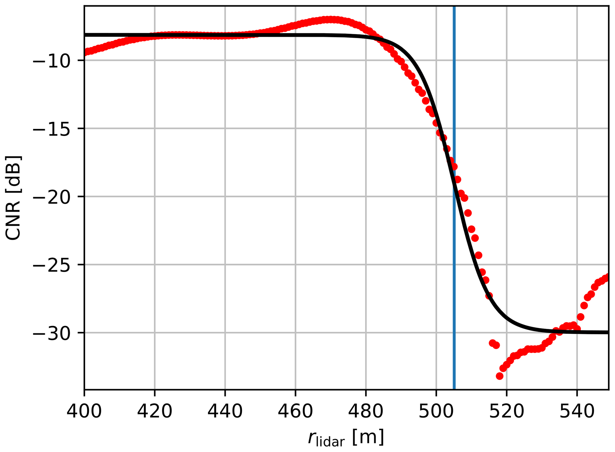
Figure 4Example of a measured CNR over the range for one azimuth angle. The black graph is an inverse sigmoid function fitted to the CNR values, and the vertical blue line is in the sigmoid's midpoint, representing the estimated distance to the sea surface.
The figure also shows an inverse sigmoid function, which was fitted to the CNR values, in black, and the midpoint of the sigmoid function is shown by the vertical line in blue, which is our estimate for the sea surface distance. For the sigmoid function we use a logistic function given by
This function is defined over the range r and is parameterized by phigh and plow for the upper and lower limit of the sigmoid, respectively, pmidpoint for the sigmoid's midpoint, and pgrowth for the logistic growth rate. The sigmoid function is fitted to the measured CNR values using a least-squares fit, and the estimate for the sea surface distance is set to
For the estimation of the distance to the sea surface we have chosen this value because at this distance the signal is partially weakened, which represents a partial absorption of the probe volume. This assumption is considered reasonable since the height of the lidar device above the still water level calculated by trigonometrical relations corresponds well with the actual height above the sea surface. Depending on the lidar instrument used and the settings, it is possible that the shape of the CNR curve will look different. In our study, the inverse sigmoid fit was found to give a robust estimate of the distance to the water surface; for other systems it may be possible that the fit function needs to be adjusted.
We only considered scans in which the CNR value exceeded a defined threshold. If the maximum CNR value for a single beam was below −18 dB for all ranges, we omitted that azimuth angle. If less than 20 azimuth angles met these requirements, we removed the entire sea surface levelling scan.
2.2.2 Sea surface distance model
To estimate the levelling of the lidar with respect to the sea surface, we built a model to calculate the distances for every azimuth angle to the surface plane for given roll and pitch angles and a height above the surface.
Figure 5 shows the definition of the coordinate system for the lidar, as well as the roll angle ρ, the pitch angle ϕ and the azimuth angle γ. Note that in this case we have defined the rotations around the axes in a clockwise direction. The following matrices define these clockwise rotations around the three axis for the substitute angle α:
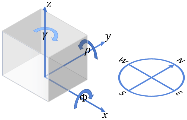
Figure 5Coordinate system of the lidar with the clockwise rotations around the axes and a compass rose. γ is the yaw angle, ρ is the roll angle, and ϕ is the pitch angle of the device.
Now we can define the building blocks for modelling the laser beam of the lidar. Without any rotations the laser beam Lscanner∈ℝ3 can be described as a three-dimensional straight line pointing to the north along the y axis by the following vector equation
where is the variable for the range.
We define the pitch with the pitch angle as follows:
The roll with the roll angle is defined as follows:
The azimuth with the azimuth angle of the scanner head is given by
We define the elevation with the elevation angle of the lidar counter-clockwise around the x axis; therefore we have to adjust the sign:
With the height of the scanner head above the sea surface we can declare the height vector H∈ℝ3:
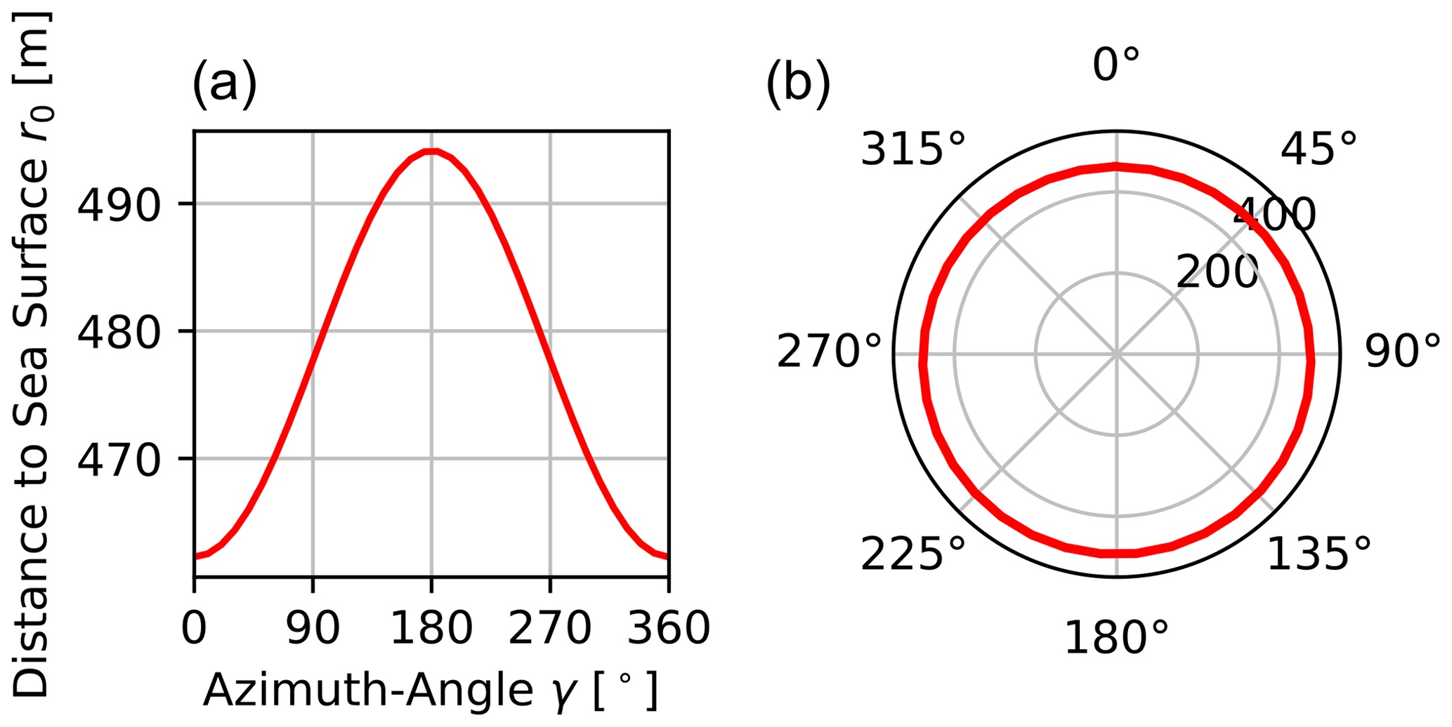
Figure 6Modelled distances to the sea surface for an example set of parameters (h=25 m, , , , ) on a regular plot (a) and a polar plot (b).
In addition, we can add the displacement vector D∈ℝ3, which consists of xshift∈ℝ and yshift∈ℝ as the shifts along the x and y axes, respectively.
For the WindCube 200S and most other long-range lidar models the laser does not exit from the centre of the rotation around the z axis since the laser is deflected by two mirrors. We did not consider this displacement in our previous work in Rott et al. (2017). Adding the displacement means that the model no longer describes a conic section and becomes more complex. However, the effects of this change are only marginal for a relatively small displacement, as is the case for a typical two-mirror lidar scanner. For this device we approximated the displacement as and yshift=0.15 m. For the sake of completeness, we list the formulas without and with the displacement and use the complete formula for our evaluation. The coordinates of the laser beam in the coordinate system of the lidar can now be described by adding the introduced displacements and rotations to Lscanner in the following manner:
We want to estimate the range at which the laser beam hits the sea surface, i.e. for the parameters and yshift. To do so, we can solve the vector equation for the variable r0 in the z coordinate. While the variable rsea (see Eq. 9) defines the measured distance to the sea surface, we introduce here the variable r0 of the modelled distance as a function of the different rotation angles and translational shifts. In our previous publication (see Rott et al., 2017), we set .
When we include the non-trivial displacement D(xshift,yshift) of the scanner head from the z axis, the complete equation for the range r0 is
Given the set of parameters and yshift we can calculate the range r0 to the sea surface.
Figure 6 illustrates the distance from the lidar to the sea surface for
h=25 m,
,
,
,
,
and
yshift=0.15 m.
2.2.3 Model fitting
To estimate the levelling of the lidar from the measured sea surface levelling scan, we have to first determine the ranges rsea(γ) to the sea surface for every viable azimuth angle γ∈Γ (see Sect. 2.2.1). Then we fit the unknown parameters () of our model from Eq. (20) to these measurements.
To do this we build an optimization problem, which minimizes the deviation of the model to the measurement data. For the cost-function we used the maximum likelihood method by utilizing the Lorentz distribution. The Lorentz distribution does not weight outliers as strongly as the commonly used Gaussian distribution, i.e. the least-squares method. The cost function is
with
The set Γ is the set of all viable azimuth angles. Hereby the optimization problem is the following:
Analogous to the previous optimization problem, we again used the Nelder–Mead method (Gao and Han, 2012) to solve this optimization.
2.3 Platform tilt model
The PTM estimates the correlation between the turbine operation and the bending of the transition piece platform. The procedure is summarized in the green boxes in Fig. 1.
We observed that the platform with the lidar was tilted, depending on the turbine operation. To consider this we assume in accordance with the elastic bending of a cantilever beam a linear rotational spring stiffness ktilt.
where τ is the tilt angle. The rotor thrust T and power P are commonly expressed as a function of the wind speed u, the swept rotor area A, air density ρ, and the dimensionless thrust and power coefficients cT and cP, respectively:
Combining Eqs. (27) to (29) yields the tilt angle as a function of the power P and the wind speed u representing temporal averages for the time during which the sea surface levelling scan was executed.
For most wind turbines the thrust and power coefficient can be approximated as constant in the variable operational speed range which corresponds to the lower to medium partial load range. Beyond and especially above the rated wind speed the dependency on the wind speed has to be considered since the thrust loading is reduced, while the rated power is maintained. In the following we consider only the variable operational speed range, typically extending between 3.5 and 9 to 11 m s−1, to simplify Eq. (30) with a constant factor c.
To define the tilt of the platform we are using the rotational matrices we defined in Sect. 2.2.2. The tilt matrix Rtilt of the platform depends on the tilt angle τ and the matrix ν in which the platform tilts (in our case this is the nacelle orientation). We define
The negative tilt angle τ has to be considered for the rotation Rx because the platform bends in the negative direction of the turbine orientation ν. This allows us to model the rotation of the platform as a combination of resting pitch and roll angles ϕr and ρr and the thrust-dependent tilt rotation of the platform.
The matrix εi is the ith residual of the combined rotations measured by the SSL in terms of the pitch angle ϕm,i and the roll angle ρm,i, as well as the modelled rotations defined by the corresponding tilt angle τm,i and orientation νm,i of the turbine, while Ω is the set of all available measurements at different operating conditions. When we substitute τm,i with the measured active power Pm,i and wind speed um,i by using Eq. (31), we are left with the three unknown parameters: c,ϕr and ρr. To estimate these parameters we try to minimize the residual εi with the following cost function:
The operator is the Frobenius norm. The optimization problem, utilizing the least-square method, then is
Again, we solved this optimization with the Nelder–Mead algorithm (Gao and Han, 2012). For the initial solution we chose and . Thus, we can determine the parameters from the measured data.
In the last step we want to utilize the obtained parameters c,ρr and ϕr to estimate the dynamic roll and pitch angles from the power and wind speed measurements of the turbine. This makes it possible to perform further lidar scans and estimate the levelling and the resulting height and position error of the lidar measurement based on the current SCADA data in post-processing. To do so we are using Eq. (33) and assume that the residual εi is zero. We rename the variables ϕm,i and ρm,i for the pitch and roll angles measured by the SSL to ϕmod,i and ρmod,i, respectively, to emphasize that in this case the variables are derived from the wind turbine data by our model.
The objective is to solve for ϕmod,i and ρmod,i. To do this, we multiply Eq. (37) with the z unit vector . Thus, the two sides of the equation represent how the rotation matrices affect the lot vector to the x–y plane, which is orthogonal to the sea surface, resulting in a unit vector n. With this we get
This can be reformulated to
Now we can derive the dynamic roll and pitch angles from the SCADA data.
2.4 Measurement set-up and data
The three methods presented in this paper refer to a measurement campaign which was carried out from August 2018 until June 2019 in the German North Sea with a scanning lidar positioned on the platform of the transition piece of a wind turbine in the offshore wind farm Global Tech I (GT I). A more detailed description of the measurement campaign is given in Schneemann et al. (2020), and some measurement data are published by Schneemann et al. (2019). In the following sections we will first present important information about the measurement set-up, equipment and the wind farm GT I (Sect. 2.4).
The offshore wind farm GT I consists of 80 turbines of the type Adwen AD 5-116 with a total nominal power output of 400 MW. It is located in the German North Sea approximately 100 km from the coast.
For the measurement campaign we had knowledge about the coordinates of all turbines, as well as a subset of 1 Hz supervisory control and data acquisition (SCADA) data, including active and reactive power output, nacelle orientation, wind speed, wind direction and turbine status.
The scanning long-range Doppler lidar we used for this investigation is a Leosphere WindCube 200S (serial number WLS200S-024) (see Fig. 7). It was installed on the transition piece platform of the turbine GT58 at the westerly border of the offshore wind farm GT I. For detailed information about the lidar, we refer to Schneemann et al. (2020).

Figure 7Image of the WindCube200S installed on the transition piece of the wind turbine in the offshore wind farm Global Tech I. Picture taken by Stephan Voß.
In the following the results of the HT, the SSL and the PTM are presented for the reference case.
3.1 Hard targeting
Since the lidar was installed on the platform southwest of the tower of wind turbine GT58, we could not see a large part of the wind farm Global Tech I (GT I) from the lidar. But the turbines north and southeast were visible. When we installed the lidar it was oriented south-southeast. We made a rough estimate for the lidar's uncorrected north orientation of and used this as our initial estimate. We defined the coordinates of the turbine GT58 as the origin of our coordinate system and used its coordinates as the initial guess for the location of the lidar, i.e. .
Figure 8 presents the results of the optimization for the whole set of available hard targets that could be detected from the lidar's position. The orange dots represent the identified hard targets. The blue symbols show the positions of the turbines. The optimization yielded , and .
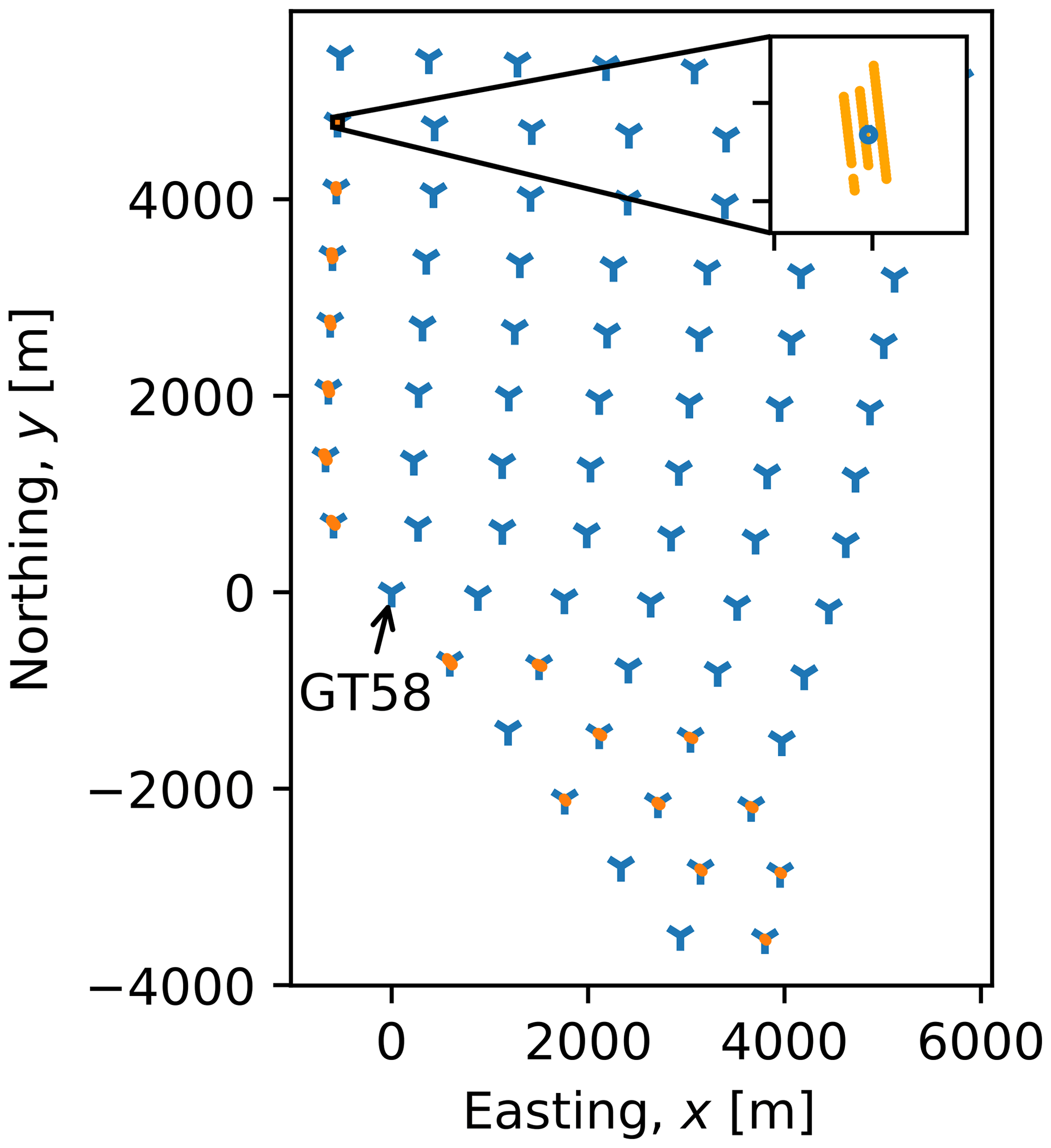
Figure 8Result of the HT. The blue symbols represent the turbine layout. The orange dots are the hard target measurements Lht. In the upper right corner is a zoom in for the northernmost hard target measurements.
For comparison, we applied HT not only to the entire set of detected wind turbines (WTs) but also to the individual WTs (Scenario 1: “individual turbines”), a subset of the various WTs located up to a certain range away from the lidar (Scenario 2: “increasing range”) and a subdivision of the WTs into northern and southern WTs from the lidar (Scenario 3: “north/south”). These three additional scenarios allowed us to observe the sensitivity of the method with respect to the set of available hard targets and their distances.
In the first scenario we applied the HT to the 17 individual turbines which could be detected from the lidar's point of view (see Fig. 8). In this case one has to be careful that the algorithm assigns the hard targets to the correct WT, since the optimization can easily converge to an incorrect WT if the initial values are not ideal. On average, this resulted in a lidar alignment of 171.71∘ with a standard deviation of 0.58∘.
In the second scenario, we artificially limited the range of the lidar. We considered six cases in which we increased the range in 1000 m increments from 1000 to 6000 m, with the goal of investigating how the results change with the addition of more hard targets.
Figure 9 shows the evolution of position determination and alignment over the range. On average, the alignment was 171.63∘ with a standard deviation of 0.02∘.
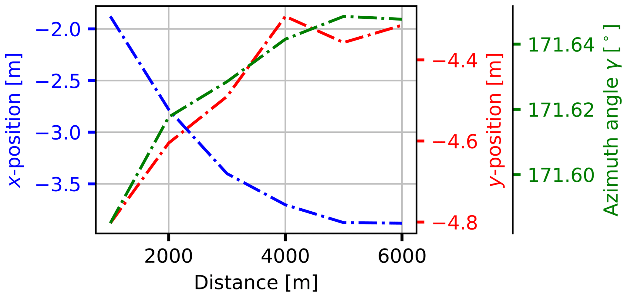
Figure 9Result of the HT for increasing range (Scenario 2). The blue graph shows the evolution of the x coordinate over the range restriction. The red graph shows the y coordinate and the green graph the azimuth angle.
In the third scenario, we divided the hard targets into two groups: those from the lidar to the north and the southern hard targets. The mean value for the alignment from these two groups is 171.65∘ with a standard deviation of 0.03∘.
In Table 1 the statistics for the three scenarios are summarized.

3.2 Sea surface levelling
3.2.1 Lidar levelling
In the first step, we determined the intersections of the laser beam of the lidar with the sea surface for the sea surface levelling scans according to Sect. 2.2.1. With the sea surface distance model (Sect. 2.2.2) we can use the optimization from Sect. 2.2.3 to find the optimal set of parameters for the height and roll angle and pitch angles. For the initial guess for our parameters we chose and .
Figure 10 illustrates an example result of the model fitting for a single SSL scan. The blue dots show estimated distances to the sea surface, which are scattered around the model fit shown in red. Some uncertainty can be seen in the measurements, but the fit still seems to reflect the distances well. The optimization for this scan yielded and hssl=24.560 m.

Figure 10Example fitting of the modelled sea surface distances to the measured distances for a complete SSL scan. and hssl=24.560 m. Illustrated in a regular plot (a) and in a polar plot (b).
We repeated this procedure for every available SSL scan from our measurement campaign (see Sect. 2.2.1). On a standard personal computer, the optimization took about 1 to 2 s to compute a suitable solution per scan. Of our measurements, 1935 scans passed our filter requirements, for which we applied the SSL.
Figures 11 and 12 display the results of our method for a consecutive subset of our measurements. Figure 11 reflects the tidal pattern in the German North Sea. As reference we also show offset-corrected Nucleus for European Modelling of the Ocean (NEMO) data (red graph) from the EU Copernicus Marine Service (, ). In Fig. 12 we can see the roll ρm and pitch ϕm angles of the lidar, which describe the levelling of the device, over the same time period. Over the entire series of measurements, larger fluctuations can be observed for both the roll angle and the pitch angle. For directly consecutive measurements, however, the fluctuations are very small in both cases. From this we conclude that the measurement noise is low, and we attribute the changes over the entire series of measurements to the variable thrust loading of the turbine at different wind speeds.
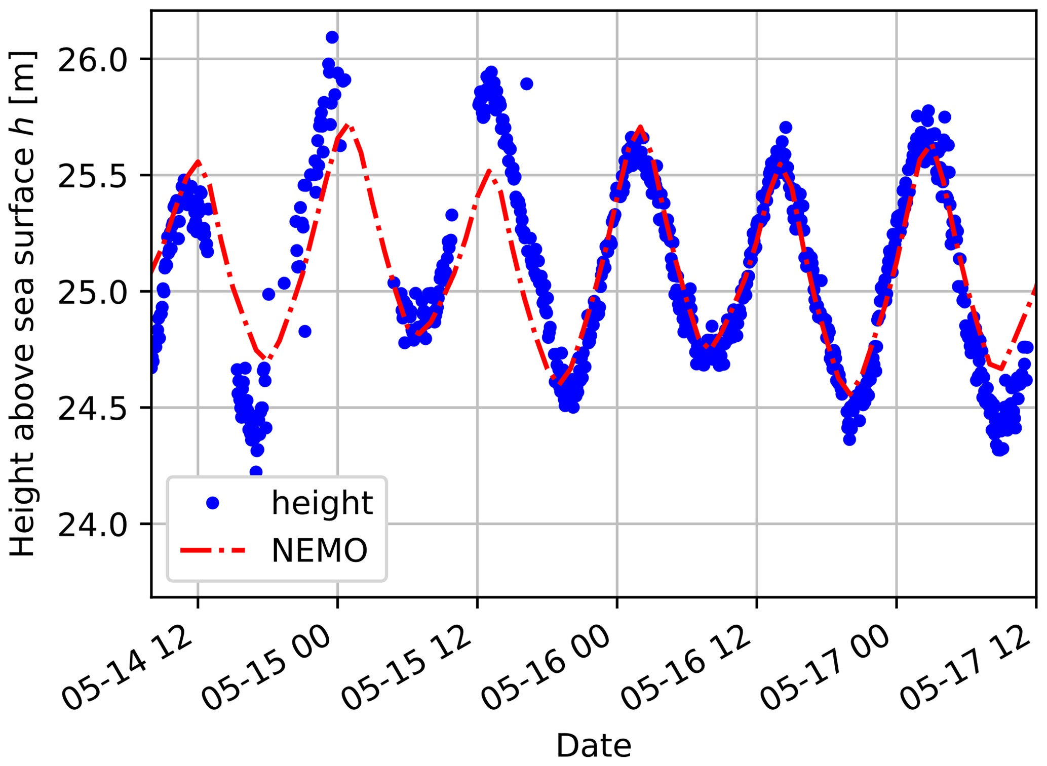
Figure 11Height above sea level determined during 3 d of continuous measurements. The blue dots represent the height of the lidar's scanning head above the sea surface as measured by SSL for a contiguous subset of the SSL scan data. Offset-corrected sea surface height from the NEMO model provided by the EU Copernicus Marine Service is shown in red.
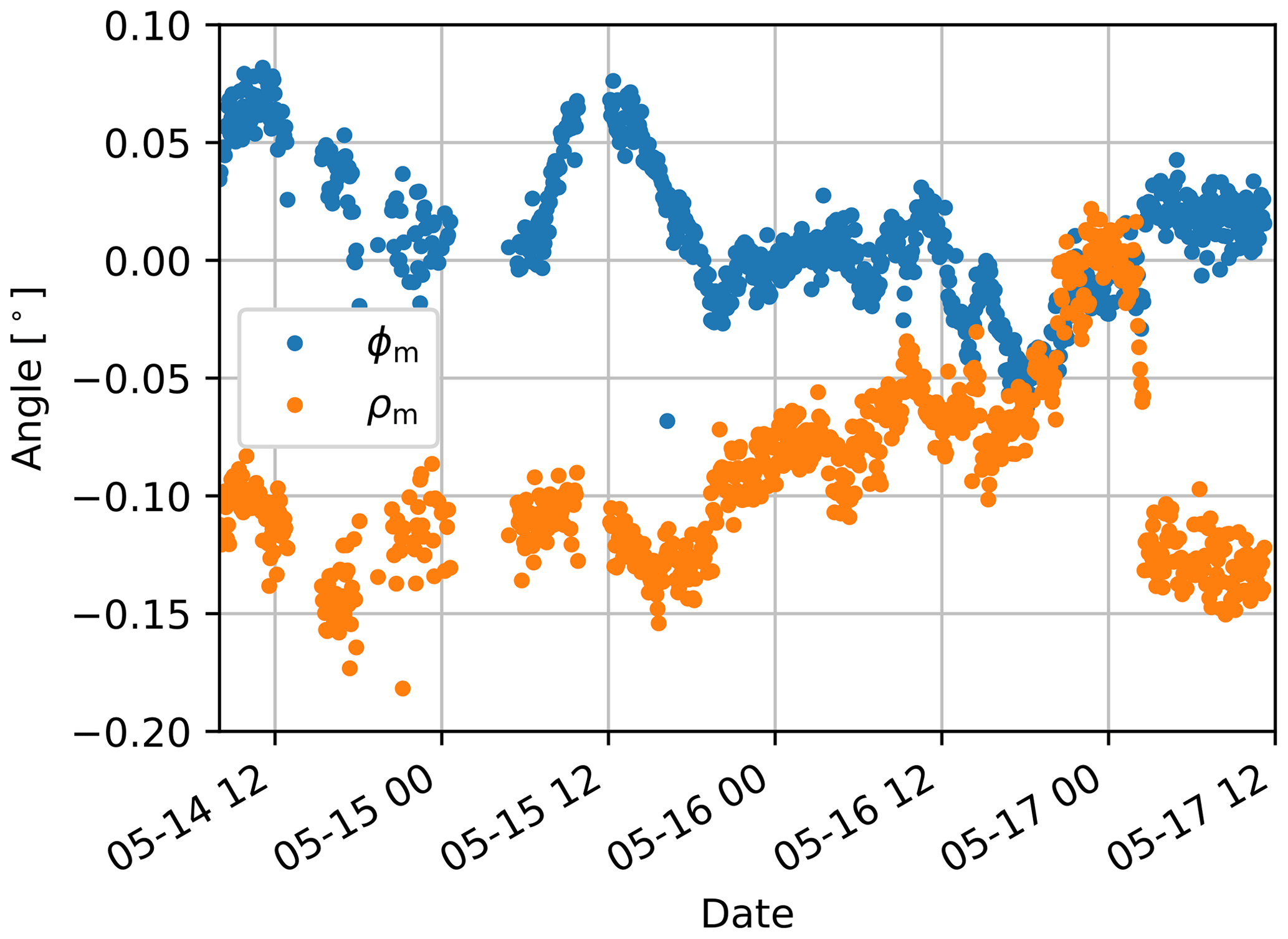
Figure 12Roll ρm and pitch ϕm angles of the lidar measured by the SSL for a contiguous subset of the SSL scan data.
3.2.2 Platform tilt angles
To easily process the results of the SSL along with the SCADA data needed to determine the platform tilt, we resampled the data to 5 min time steps using 5 min averages. With this we have a joined set of 1142 measurements. After fitting the PTM to the measurements we achieved the following results for the three parameters:
The parameter c allows us to estimate the tilt angle of the transition piece platform according to Eq. (31).
In Fig. 13 a comparison of the estimated tilt angles is depicted for all joined measurements. The black dots show the tilt angle calculated by the PTM with the SCADA data. We refer to this as the modelled tilt angle τmod. The red dots show the tilt angle of the lidar derived from the roll ρm and pitch ϕm angles measured by the SSL using Eq. (33) and the estimated resting roll ρr and pitch ϕr angles by minimizing the residual εi. We refer to this as the measured tilt angle τm.
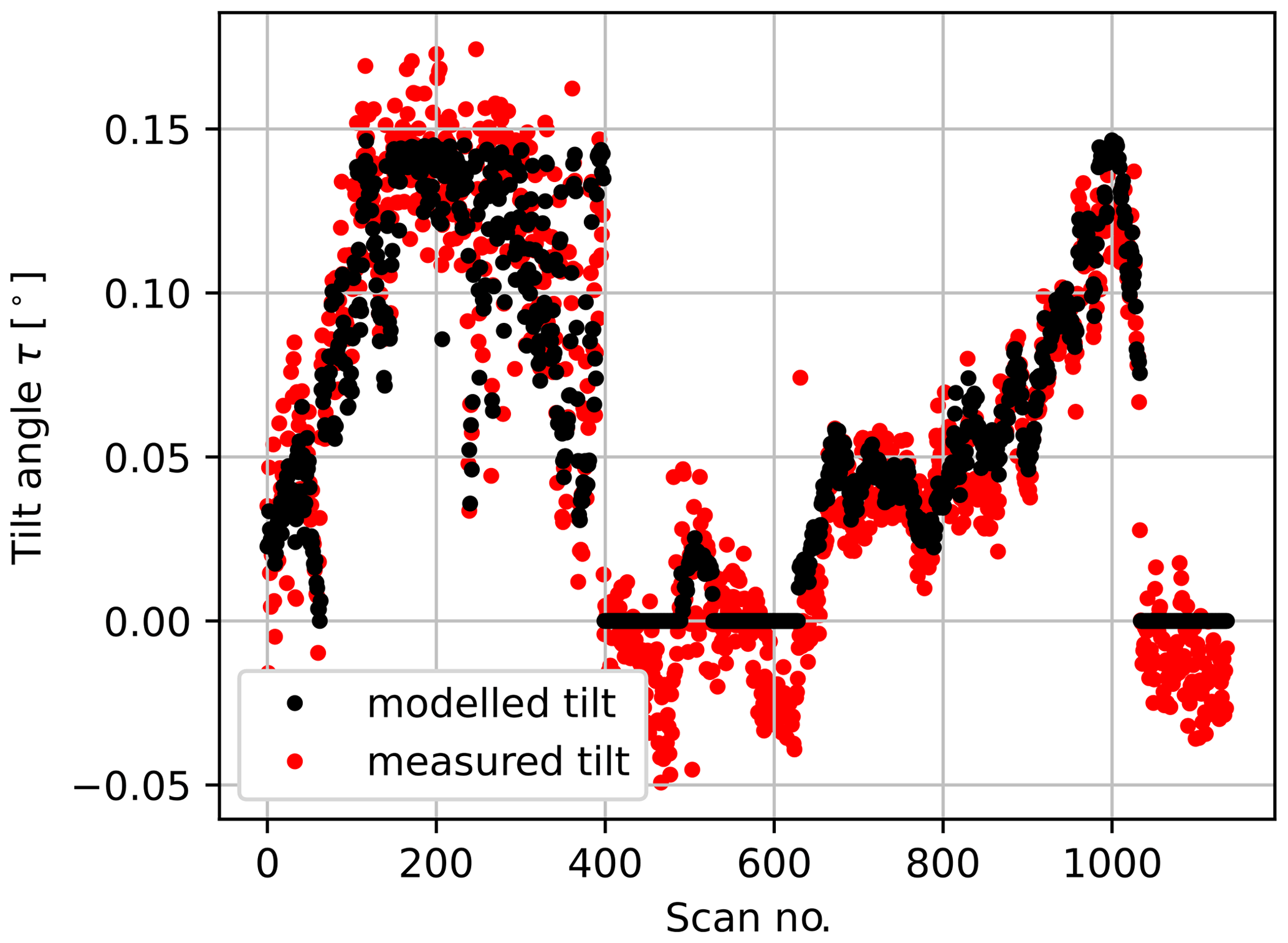
Figure 13Comparison of the measured tilt angle τm (red) derived from the roll ρm and pitch ϕm angles measured by the SSL and the modelled tilt angle τmod estimated by the PTM (black) over the scan number.
The maximum modelled tilt angle is around 0.14∘ when the turbine is in normal operation and the wind speed is close to the nominal wind speed. There are a few periods when the estimation of the PTM yields 0∘. They coincide with situations without power production and associated thrust loading. In these situations the measured tilt angle drops below 0∘. We believe that the weight of the rotor pulls the tower and consequently the transition piece platform forward, creating a negative tilt angle. However, the amount is relatively small. Therefore, we have not refined the model in this respect.
In Fig. 14 the measured tilt angle and the modelled tilt angle are compared in a scatter plot to demonstrate the strong linear correlation between our thrust estimation (see Eq. 31) and the tilting of the transition piece platform.
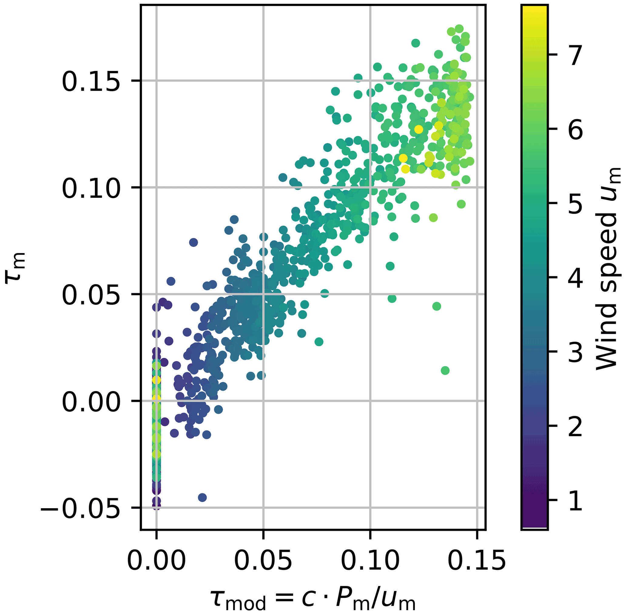
Figure 14Comparison of the modelled tilt angle τmod of the transition piece platform estimated by the PTM (x axis) to the measured tilt angle τm derived from the roll ρm and pitch ϕm angles measured by the SSL (y axis) in a scatter plot. The colour of the scatter points represent the wind speed measured by the turbine anemometer.
In Fig. 15 we can see the modelled roll and pitch angles in comparison to the values measured by the SSL. We obtain them by inserting the estimated parameters into Eq. (38) and then using Eq. (39). A few instances can be observed in which the modelled angles remain temporarily constant at their resting positions ρr and ϕr. These are situations in which the turbine has not produced any power; thus the thrust in our model has been set to 0 kN, and thereby the tilt angle is also 0∘.
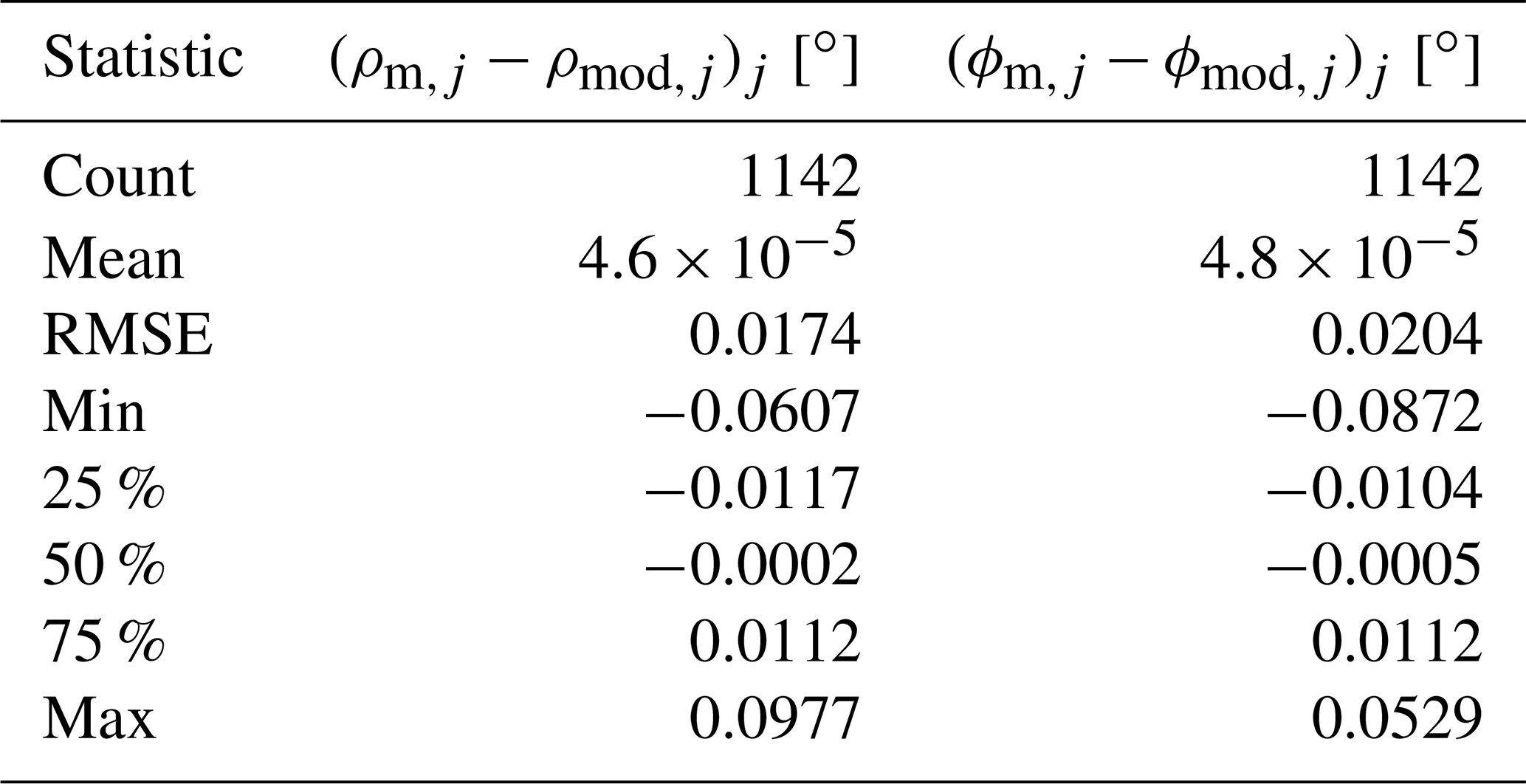
Table 2 summarizes the statistical deviations between the measured and the modelled roll and pitch angles. The table shows the number of measurements (count), the average deviation (mean), the root mean square error of the estimate (RMSE), the largest negative deviation between the measured and the modelled angles (min), the lower quartile of the error (25 %), the median (50 %), the upper quartile (75 %), and the largest position deviation of the measured and the modelled angles (max) for the roll and the pitch angle.
The hard targeting scans and sea surface levelling scans are very valuable measurements for an offshore lidar campaign. They do not require additional equipment and only take a rather small amount of time but can help improve the accuracy of the measurement campaign significantly. The knowledge of the correct orientation and position of the lidar is essential for measurement campaigns in which local effects, e.g. turbine wake and induction zone, are analysed. Information about the levelling of the device is useful for all measurements but especially for long-range measurements since the error in measurement height due to a misalignment scales linearly with the range.
HT to determine the north alignment and position of a long-range lidar is a commonly used technique that probably evolved from cross bearing in navigation and is based on standard geometry. Nevertheless, we have not found a consistent description of the method in the literature that relates to the calibration of long-range Doppler wind lidars and can be easily applied in a wind farm. Therefore, we wanted to dedicate a small part of this paper to the presentation of a simple method that can accurately determine the position of the lidar in addition to the north orientation. In our study we applied the method to a subset of the available hard targets in three different scenarios to investigate the sensitivity of the method towards the amount of suitable data.
In Scenario 1 we applied the HT to the 17 individual wind turbines we could detect in the hard target scans and computed mean and standard deviation of the orientation and positioning. The results show that the method is not very accurate when applied to individual turbines. Especially in the case of positioning, there are larger deviations in the results. This is due to the fact that the detection of individual hard targets is not very accurate because of probe length averaging. In addition, only the coordinates corresponding to the centre of the tower were available for the individual turbines. Unfortunately, no statement could be made about the accuracy of these coordinates.
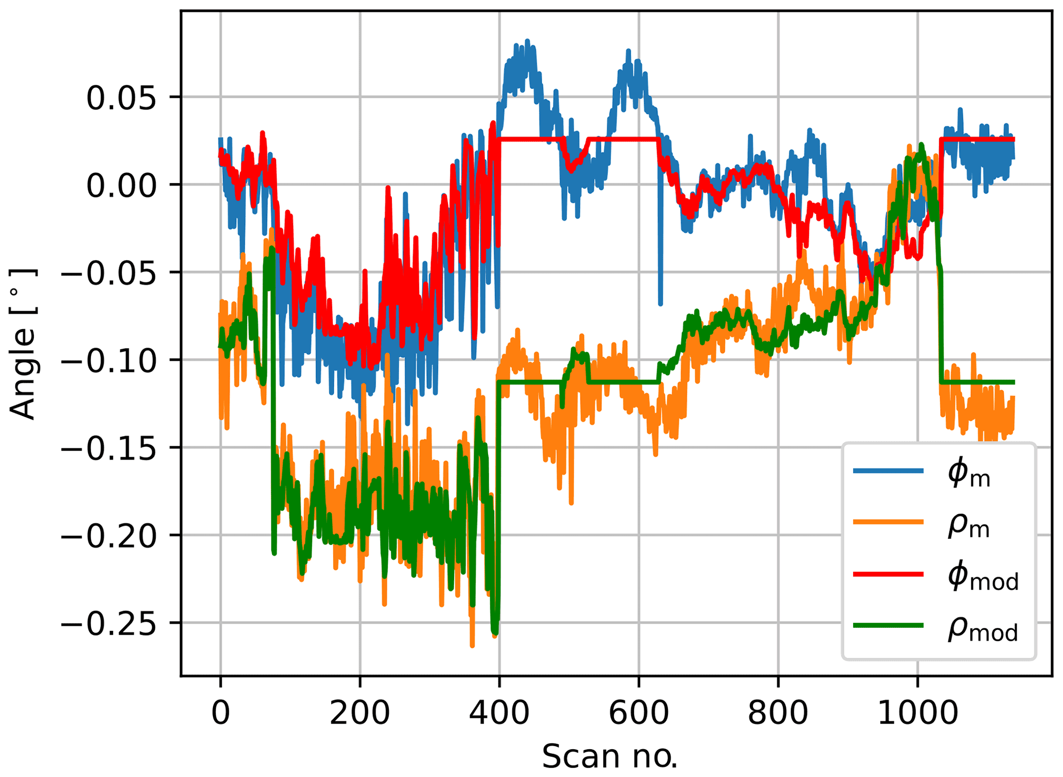
Figure 15Comparison of the roll ρm and pitch ϕm angles measured by the SSL and the roll ρmod and pitch ϕmod angles modelled by the PTM.
Table 2Error statistics of the modelled roll and pitch angles to the measured roll and pitch angles.
In Scenario 2, the method was applied to hard targets within a certain measurement range. The range was successively increased until all available data were included. This example demonstrates how adding additional hard targets ensures that the results for positioning and alignment each converge to a constant value.
In the third scenario, the set of available hard targets was divided into the northern and southern turbines when viewed from the lidar. The results show that the orientation is determined almost identically for both subsets, but there are differences of several metres in the positioning. This is due to the fact that for both subsets the vectors to the respective hard targets are almost linearly dependent on each other. For a more precise positioning, reference points are needed which are located in as different directions as possible (ideally orthogonal to each other).
Overall, the accuracy of the determination of position and orientation by the method presented here increases with the number of hard targets detected. The results from Scenario 2 show that especially the determination of the orientation has a very high accuracy.
In connection with hard target scans, it is recommended to investigate the pointing accuracy of the lidar's scanner unit as discussed in Vasiljevic (2014). Depending on the device or device type, there may be different sources of inaccuracies, such as the backlash problem. It is therefore advisable to quantify such errors before a hard target scan by performing scans with different scan speeds or scan rotation directions.
The SSL is a rather new technique, which was first introduced in Rott et al. (2017). In this paper we extended the method and explained it in more detail. The advantage of this method is that by only using the lidar itself and the sea surface, it reaches a very high accuracy in determining the levelling. Since the laser itself is utilized, this is even an advantage over additional alignment sensors attached to the lidar's housing.
Figure 6 shows that a misalignment of 0.1∘ leads to a maximum difference in distance of more than 30 m for the given set-up. This demonstrates the sensitivity of the shape of the intersection with regards to the pitch angle of the lidar device. This sensitivity strongly depends on the elevation angle of the PPI scan. Here we have chosen an angle of based on experience from previous campaigns. A smaller absolute angle further increases the sensitivity of the intersection shape, but this also increases the uncertainties caused by waves. In general, the elevation must be chosen to match the measurement set-up, the most important thing being that there is a direct line of sight to the water surface for as large a sector as possible. The setting of the range gates should also be selected carefully. In our case, we chose a 1 m resolution that sufficiently resolves the drop in CNR value at which the beam hits the water (see Fig. 4).
A large source of uncertainty is the determination of the distance to the sea surface (Sect. 2.2.1). It is possible that the method presented here systematically overestimates or underestimates the distances. However, as long as this is done consistently, only the size but not the general shape of the intersection with the water surface is affected by this. This leads to an error in the estimation of the height but not in the estimation of the angles. Due to the flat elevation angle, an over- or underestimation of the distance by, for example, 20 m results in an over- or underestimation of the height above the water surface by approx. 1 m. Another source of uncertainty in the determination of the distance to the sea surface are waves, thus the best time for the SSL scan is when the water surface is very calm. However, the effects of a misaligned lidar are so significant that we perceive the influence of the waves as measurement uncertainty, which is largely averaged out in the measurements. A further source for the deviation of the measured distances and the model fitting, which can be observed in Fig. 10, is movement of the transition piece platform during an SSL scan. With our set-up one SSL scan took approximately 5 min to execute; therefore fluctuations with a higher frequency change the shape of the intersection of the laser beam with the sea surface. This is not considered in the model fitting. The SSL as described here therefore gives an average value for the levelling over the scan duration. Furthermore, the movement of the transition piece platform is only modelled as a rotation at the scanner head. It is likely that the origin of the rotation for the tilt is located further below, resulting in movement of the lidar. However, since the angles are relatively small, the motion is primarily lateral and does not affect the distances to the sea surface; only the change in height due to bending of the tower base directly affects the distance to the sea surface. Since these changes are very small and, moreover, the point of origin cannot be accurately determined, we have neglected this. Lastly, the accuracy of the model fitting also depends on the quality of the SCADA data. Especially the nacelle orientation has an important role for the thrust model. A deviation in the measurement of the nacelle orientation leads to a systematic error in the tilt model. For our measurement campaign we checked this sensor and assumed that the error or the orientation of the turbine is within 2∘.
Nevertheless, the results of the SSL are considered very reliable. This is supported by the fact that successive measurements for levelling lead to very similar results, which can be seen in Fig. 12. In addition, the temporal development of the roll and pitch angles can be described on average very well by means of the PTM (see Fig. 15). If we look at the results in Table 2, we can see that the RMSE is only about 0.02∘ for both roll and pitch. We assume that the total model error is of the same order of magnitude. Without power output the turbine's thrust model yields zero loading, and the modelled angles take their resting position. In Fig. 15 we can observe periods when this occurs, and the modelled roll and pitch angles are constant. In these situations we can clearly see a deviation to the measured values, and therefore the thrust model does not seem to work that well. This is probably because a turbine also exerts wind loading when it is not producing power, and even if the wind speed and therefore the thrust are very low, the tower top tilt moment due to the excentric weight of the rotor-nacelle assembly can lead to an inclination of the transition piece platform, which is not considered in our tilt model. In this respect, the model could be improved in the future.
SSL allows us to determine the levelling of a lidar. Thereby larger inclinations can be identified and corrected at the beginning of a measurement campaign. But even if a correction is not possible for logistic reasons and, as we discovered, dynamic variations of the levelling occur, it is helpful to know the exact orientation of a lidar so that the measurements can be interpreted accordingly, as was done in Schneemann et al. (2021). To illustrate, we consider an example of the effects that inclinations can have on measurements. In our measurement campaign we observed a maximum absolute roll angle of about 0.25∘ (see Fig. 15). This angle alone, for a horizontal PPI scan, causes the height of measurements at 1 km distance to be wrong by up to approx. 4.4 m depending on the azimuth angle. For typical long-range lidars measuring up to 8 km, this builds up to about 35 m, which is more than the height above the water surface of about 25 m for our measurement campaign. This means that at a distance of about 6.5 km we would have hit the sea surface at a downward inclination (Earth curvature taken into account), while at an upward inclination we would have more than doubled the measurement height.
The transition piece platform in our measurement campaign was mounted on a tripod with a water depth of about 40 m. Even though the water depth is comparatively large, we would expect that even larger tilt angles can occur at wind turbines that are mounted on a more flexible monopile and probably even larger at floating wind turbines. For nacelle-based lidar measurements the movement of the nacelle is in the order of 1 to 2∘. This emphasizes the importance of knowing the correct alignment. We think that in the future additional sensors should be utilized that can directly measure the levelling of the lidar with high accuracy. These should be compared to the results of the SSL, thus providing a reference for the alignment of the laser with which the correct installation of the sensor can be verified. Until then, we recommend performing the HT at the beginning of a measurement campaign to correct the orientation. Afterwards, the SSL should be run continuously to determine the levelling and to obtain sufficient data for the parameterization of the PTM. During the campaign, it is recommended to repeat the SSL from time to time to check if the parameterization is still acceptable and the levelling of the lidar is still correct.
Furthermore, it should be explored how information from such sensors can be directly incorporated into the lidar control to dynamically correct the elevation of the scanner head, or whether it is possible to mount the lidar or the scanner of the lidar in a Cardan suspension.
The objectives of this paper were to present two methods for accurately estimating the position, orientation and levelling of a long-range lidar in an offshore environment and in addition to introduce a model that can estimate turbine-induced inclinations from turbine operating data. This information can be used to correct the position data of the measuring points of ongoing lidar measurements. On the one hand, a more precise orientation of the lidar helps to transfer the measurement points more accurately into the global coordinate system, and, on the other hand, it provides a better estimate of the actual height at which the wind speed was measured by a lidar. This helps to reduce uncertainties in long-range-scanning lidar data analysis.
HT, SSL and the PTM are described in detail and applied to data from an offshore measurement campaign. For HT, we have shown that the presented method takes advantage of detecting multiple hard targets in different directions, thereby increasing the accuracy. While we assume an error of about 1 m for the positioning of the instrument, the northing results in consistent values, which indicate a very high accuracy (see Table 1). For SSL and the PTM, the evaluations (Table 2) show that the inclinations measured by the SSL can be reproduced by the PTM with a very high accuracy. In addition, the SSL also provides a good estimation of the water surface height.
The HT is not limited to being used offshore and should be applied to every long-range lidar campaign to estimate the orientation and positioning at the start of a measurement campaign. While the PTM presented here was developed specifically for use of a lidar on the platform of a transition piece, it can be extended to other offshore sites where tilt is related to the thrust of the wind turbine.
In general, knowledge about the positioning, orientation and levelling of remote sensing equipment is crucial for successful measurements at longer distances. We therefore consider it very important to perform calibration measurements as proposed in this paper during each measurement campaign.
The code and scripts developed in this research are published at the following: https://doi.org/10.5281/zenodo.5654919 (Rott et al., 2021b).
The data used for the evaluation can be used as an illustration of the code and can be found here: https://doi.org/10.5281/zenodo.5654866 (Rott et al., 2021a).
AR initiated and directed the research, developed the methods, prepared the computational scripts, analysed the measured data, was heavily involved in funding acquisition and research discussion, prepared the figures, and was lead author of the article. JS assisted with data provision and data processing, as well as derivation of the methods, and provided extensive feedback in several reviews. FT assisted in the development of the computational scripts, verified the calculations, provided support in countless discussions and gave extensive feedback in several interactions. JJTQ supported with his rich experience of lidar systems, was instrumental in drafting the research question and helped with extensive review. MK was instrumental in acquiring funding, supervised the research, and provided support with valuable comments and good advice.
The contact author has declared that neither they nor their co-authors have any competing interests.
Publisher’s note: Copernicus Publications remains neutral with regard to jurisdictional claims in published maps and institutional affiliations.
We acknowledge the wind farm operator Global Tech I Offshore Wind GmbH for providing SCADA data, as well as their support of the work and the measurement campaign. Thanks to EU Copernicus Marine Service Information for providing sea surface height data from the NEMO model used in Fig. 11. Special thanks to Johannes Schulz-Stellenfleth, Helmholtz Zentrum Geesthacht, for helping with sea surface height data. Many thanks to Thomas Luhmann, Jade University of Applied Sciences, for the useful comments and advice. Special thanks to Stephan Voß, ForWind – University Oldenburg, for his work and support in planning and conducting the measurement campaign.
We performed the lidar measurements and parts of the work in the framework of the research projects “OWP Control” (grant no. FKZ 0324131A) and “X-Wakes” (grant no. FKZ 03EE3008D), both funded by the German Federal Ministry for Economic Affairs and Energy on the basis of a decision by the German Bundestag. The work of Frauke Theuer has been supported by the German Federal Environmental Foundation (DBU) (grant no. 20018/582).
This paper was edited by Jakob Mann and reviewed by two anonymous referees.
Bromm, M., Rott, A., Beck, H., Vollmer, L., Steinfeld, G., and Kühn, M.: Field investigation on the influence of yaw misalignment on the propagation of wind turbine wakes, Wind Energy, 21, 1011–1028, https://doi.org/10.1002/we.2210, 2018. a
Gao, F. and Han, L.: Implementing the Nelder-Mead simplex algorithm with adaptive parameters, Comput. Optim. Appl., 51, 259–277, 2012. a, b, c
Gottschall, J., Wolken-Möhlmann, G., Viergutz, T., and Lange, B.: Results and conclusions of a floating-lidar offshore test, Energy Proced., 53, 156–161, https://doi.org/10.1016/j.egypro.2014.07.224, 2014. a
Koch, G. J., Beyon, J. Y., Modlin, E. A., Petzar, P. J., Woll, S., Petros, M., Yu, J., and Kavaya, M. J.: Side-scan Doppler lidar for offshore wind energy applications, J. Appl. Remote Sens., 6, 1–11, https://doi.org/10.1117/1.jrs.6.063562, 2012. a
Krishnamurthy, R., Boquet, M., and Osler, E.: Current Applications of Scanning Coherent Doppler Lidar in Wind Energy Industry, in: EPJ Web of Conferences, EDP Sciences, 119, 10003, https://doi.org/10.1051/epjconf/201611910003, 2016. a
Krishnamurthy, R., Reuder, J., Svardal, B., Fernando, H., and Jakobsen, J.: Offshore Wind Turbine Wake characteristics using Scanning Doppler Lidar, Energy Proced., 137, 428–442, https://doi.org/10.1016/j.egypro.2017.10.367, 2017. a
Madec, G., Bourdallé-Badie, R., Chanut, J., Clementi, E., Coward, A., Ethé, C., Iovino, D., Lea, D., Lévy, C., Lovato, T., Martin, N., Masson, S., Mocavero, S., Rousset, C., Storkey, D., Vancoppenolle, M., Müeller, S., Nurser, G., Bell, M., and Samson, G.: NEMO ocean engine, Zenodo [code], https://doi.org/10.5281/zenodo.1464816. a
Pichugina, Y. L., Brewer, W. A., Banta, R. M., Choukulkar, A., Clack, C. T. M., Marquis, M. C., McCarty, B. J., Weickmann, A. M., Sandberg, S. P., Marchbanks, R. D., and Hardesty, R. M.: Properties of the offshore low level jet and rotor layer wind shear as measured by scanning Doppler Lidar, Wind Energy, 20, 987–1002, https://doi.org/10.1002/we.2075, 2016. a
Rott, A., Schneemann, J., Trabucchi, D., Trujillo, J. J., and Kühn, M.: Accurate deployment of long range scanning lidar on offshore platforms by means of sea surface leveling, in: Poster presentation Windtech 2017, available at: http://windtechconferences.org/wp-content/uploads/2018/01/Windtech2017_AnRott-Poster.pdf (last access: 6 February 2018), 2017. a, b, c, d
Rott, A., Schneemann, J., and Theuer, F.: Data supplement for “Alignment of scanning lidars in offshore wind farms” – Wind Energy Science Journal, Zenodo [data set], https://doi.org/10.5281/zenodo.5654866, 2021a. a, b
Rott, A., Schneemann, J., and Theuer, F.: AndreasRott/Alignment_of_scanning_lidars_in_offshore_wind_farms: Version1.0, Zenodo [code], https://doi.org/10.5281/zenodo.5654919, 2021b. a, b
Schneemann, J., Voß, S., Rott, A., and Kühn, M.: Doppler wind lidar plan position indicator scans and atmospheric measurements at the offshore wind farm “Global Tech I”, ForWind, Institute of Physics, Carl-von-Ossietzky University Oldenburg, Pangaea, https://doi.org/10.1594/PANGAEA.909721, 2019. a
Schneemann, J., Rott, A., Dörenkämper, M., Steinfeld, G., and Kühn, M.: Cluster wakes impact on a far-distant offshore wind farm's power, Wind Energ. Sci., 5, 29–49, https://doi.org/10.5194/wes-5-29-2020, 2020. a, b, c
Schneemann, J., Theuer, F., Rott, A., Dörenkämper, M., and Kühn, M.: Offshore wind farm global blockage measured with scanning lidar, Wind Energ. Sci., 6, 521–538, https://doi.org/10.5194/wes-6-521-2021, 2021. a, b
Shimada, S., Goit, J. P., Ohsawa, T., Kogaki, T., and Nakamura, S.: Coastal Wind Measurements Using a Single Scanning LiDAR, Remote Sens., 12, 1347, https://doi.org/10.3390/rs12081347, 2020. a
Theuer, F., van Dooren, M. F., von Bremen, L., and Kühn, M.: Minute-scale power forecast of offshore wind turbines using long-range single-Doppler lidar measurements, Wind Energ. Sci., 5, 1449–1468, https://doi.org/10.5194/wes-5-1449-2020, 2020. a
Trujillo, J.-J., Cañadillas, B., Ehmsen, A., and Neumann, T.: Measuring effects of the Borkum Riffgrund 1 wind farm on FINO1 by means of long range lidar, in: Wind Europe Offhshore, 26–28 November 2018, Copenhagen, Denmark, PO166, https://windeurope.org/offshore2019/conference/posters/(last access date: 29 January 2022), 2019. a, b
Trujillo, J.-J., Orozco, P., Cañadillas, B., Frühmann, R., and Neumann, T.: Assessment of representative wind speed vertical profiles in the vicinity of offshore windfarms by means of long-range lidar, in: EERA-DeepWind Conference, 13–15 January 2021, https://www.sintef.no/globalassets/project/eera-deepwind-2021/presentasjoner/c-trujillo-juan_ul-international.pdf (last access: 29 January 2022), 2021. a
Vasiljevic, N.: A time-space synchronization of coherent Doppler scanning lidars for 3D measurements of wind fields, PhD thesis, DTU Wind Energy, available at: https://orbit.dtu.dk/files/102963702/NVasiljevic_Thesis.pdf (last access: 29 January 2022), 2014. a, b
Virtanen, P., Gommers, R., Oliphant, T. E., Haberland, M., Reddy, T., Cournapeau, D., Burovski, E., Peterson, P., Weckesser, W., Bright, J., van der Walt, S. J., Brett, M., Wilson, J., Jarrod Millman, K., Mayorov, N., Nelson, A. R. J., Jones, E., Kern, R., Larson, E., Carey, C., Polat, l., Feng, Y., Moore, E. W., Vand erPlas, J., Laxalde, D., Perktold, J., Cimrman, R., Henriksen, I., Quintero, E. A., Harris, C. R., Archibald, A. M., Ribeiro, A. H., Pedregosa, F., van Mulbregt, P., Vijaykumar, A., Bardelli, A. P., Rothberg, A., Hilboll, A., Kloeckner, A., Scopatz, A., Lee, A., Rokem, A., Nathan Woods, C., Fulton, C., Masson, C., Häggström, C., Fitzgerald, C., Nicholson, D. A., Hagen, D. R., Pasechnik, D. V., Olivetti, E., Martin, E., Wieser, E., Silva, F., Lenders, F., Wilhelm, F., Young, G., Price, G. A., Ingold, G.-L., Allen, G. E., Lee, G. R., Audren, H., Probst, I., Dietrich, J. P., Silterra, J., Webber, J. T., Slavič, J., Nothman, J., Buchner, J., Kulick, J., Schönberger, J. L., de Miranda Cardoso, J. V., Reimer, J., Harrington, J., Cano Rodríguez, J. L., Nunez-Iglesias, J., Kuczynski, J., Tritz, K., Thoma, M., Newville, M., Kümmerer, M., Bolingbroke, M., Tartre, M., Pak, M., Smith, N. J., Nowaczyk, N., Shebanov, N., Pavlyk, O., Brodtkorb, P. A., Lee, P., McGibbon, R. T., Feldbauer, R., Lewis, S., Tygier, S., Sievert, S., Vigna, S., Peterson, S., More, S., Pudlik, T., Oshima, T., Pingel, T. J., Robitaille, T. P., Spura, T., Jones, T. R., Cera, T., Leslie, T., Zito, T., Krauss, T., Upadhyay, U., Halchenko, Y. O., and Vázquez-Baeza, Y.: SciPy 1.0: Fundamental Algorithms for Scientific Computing in Python, Nat. Methods, 17, 261–272, https://doi.org/10.1038/s41592-019-0686-2, 2020. a