Data-driven farm-wide fatigue estimation on jacket-foundation OWTs for multiple SHM setups

The sustained development over the past decades of the offshore wind industry has seen older wind farms beginning to reach their design lifetime. This has led to a greater interest in wind turbine fatigue, the remaining useful lifetime and lifetime extensions. In an attempt to quantify the progression of fatigue life for offshore wind turbines, also referred to as a fatigue assessment, structural health monitoring (SHM) appears as a valuable contribution. Accurate information from a SHM system can enable informed decisions regarding lifetime extensions. Unfortunately direct measurement of fatigue loads typically revolves around the use of strain gauges, and the installation of strain gauges on all turbines of a given farm is generally not considered economically feasible. However, when we consider that great numbers of data, such as supervisory control and data acquisition (SCADA) and accelerometer data (of cheaper installation than strain gauges), are already being captured, these data might be used to circumvent the lack of direct measurements.

It is then highly relevant to know what is the minimal sensor instrumentation required for a proper fatigue assessment. In order to determine this minimal instrumentation, a data-driven methodology is developed for real-world jacket-foundation offshore wind turbines (OWTs). In the current study the availability of high-frequency SCADA (1 Hz) and acceleration data (>1 Hz) as well as regular 10 min SCADA is taken as the starting point. Along these measured values, the current work also investigates the inclusion of an estimate of the quasi-static thrust load using the 1 s SCADA using an artificial neural network (ANN).

After data collection all data are transformed to features on a 10 min interval (feature generation). When considering all possible variations a total of 430 features was obtained. To reduce the dimensionality of the problem this work performs a comparative analysis of feature selection algorithms. The features selected by each method are compared and related to the sensors to decide on the most cost-effective instrumentation of the OWT.

The variables chosen by the best-performing feature selection algorithm then serve as the input for a second ANN, which estimates the tower fore–aft (FA) bending moment damage equivalent loads (DELs), a valuable metric closely related to fatigue. This approach can then be understood as a two-tier model: the first tier concerns itself with engineering and processing 10 min features, which will serve as an input for the second tier that estimates the DELs.

It is this two-tier methodology that is used to assess the performance of eight realistic instrumentation setups (ranging from 10 min SCADA to 1 s SCADA, thrust load and dedicated tower SHM accelerometers). Amongst other findings, it was seen that accelerations are essential for the model's generalization. The best-performing instrumentation setup is looked at in greater depth, with validation results of the tower FA DEL ANN model showing an accuracy of around 1 % (MAE) for the training turbine and below 3 % for other turbines, with a slight underprediction of fatigue rates. Finally, the ANN DEL estimation model – based on two intermediate instrumentation setups (combinations of 1 s SCADA, thrust load, low quality accelerations) – is employed in a farm-wide setting, and the probable causes for outlier behaviour are investigated.

1 Introduction

1.1 Fatigue assessment

Topics such as the fatigue experienced by offshore wind turbines, their remaining useful lifetime and foreseeable lifetime extensions have become increasingly crucial for the offshore wind energy sector, particularly as older wind farms begin to reach the end of their design lifetime. Taking into account the fatigue assessment of turbines is fundamental if operators are to make informed decisions regarding wind turbine's lifetime extension. Collecting data required for such fatigue assessments is generally considered a part of structural health monitoring (SHM). Martinez-Luengo and Shafiee (2019) have shown how, although initially increasing the capital expenditures as some additional hardware is required, SHM induces a reduction in operational expenditure which far exceeds the initial increase in capital expenditures. Thus, SHM is highly attractive in the current industry climate, as it allows us to reduce overall costs, which can then be translated into a further reduction of the cost of energy (CoE), one of the main challenges of the industry at large (van Kuik et al., 2016). Furthermore, offshore wind turbine design is usually driven by fatigue, wherein improvements in fatigue assessment of built wind turbines can induce further optimization of future designs (Seidel et al., 2016).

Fatigue assessments are often based on measurements of the turbine's load history (Loraux and Brühwiler, 2016; Schedat et al., 2016; Iliopoulos et al., 2017; Ziegler et al., 2017). A direct measurement of fatigue loads is obtained through the use of strain gauges. Strain gauges on the substructure's primary steel allow us to measure the strain histories. These strain histories can then be readily translated to stress histories and ultimately fatigue loads, e.g. through the use of a rainflow-counting algorithm. Unfortunately, the installation and operation of strain gauges is rather labour and maintenance intensive, resulting in a rather limited industry adoption. At best, only a subset of turbines in a farm are equipped with strain gauges to monitor the fatigue life of the substructure. In contrast, operators do want to understand the fatigue rates across the entire wind farm, and as such alternatives to quantify fatigue loads are being searched. In particular the use of supervisory control and data acquisition (SCADA) data is often considered. SCADA data are interesting as they capture the key operational data (i.e. power production, wind speed, blade pitch, etc.) of an offshore wind turbine. SCADA is also available for every turbine and is stored by most operators. When a method can be developed that estimates fatigue rates from SCADA data, then farm-wide fatigue rates can be obtained.

However, for offshore wind turbines the sole use of SCADA data might be insufficient to fully explain fatigue behaviour. While the turbine control and environmental conditions cover a significant part of fatigue loads, the interaction between dynamic loads and the structural dynamics of the substructure also plays a key role (Vorpahl et al., 2013). It is this interaction that is typically poorly represented by the SCADA data¹. In contrast, accelerometer data almost exclusively cover those structural dynamics and are closely related to the stress histories. We can see how closely related the accelerometer data are to the strain measurements in Fig. 1. Therefore the inclusion of accelerometer data is considered to complement SCADA data.

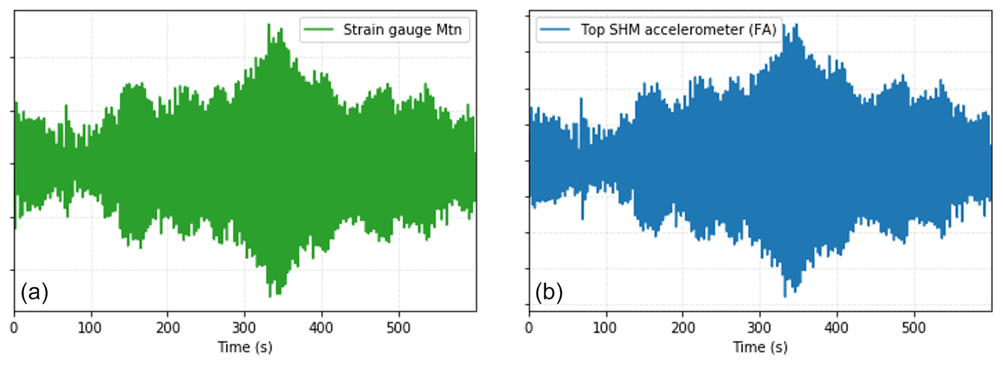
Figure 1 (a) Fore–aft bending moment (M_tn, Nm) signal, measured by the strain gauges during a standstill occurrence of 600 s. (b) Top tower SHM accelerometer fore–aft displacement signal (m) for the same period as in panel (a).

In this contribution, we investigate a solution to estimate the fatigue rates (expressed as damage equivalent loads, DEL) for an offshore wind farm on jacket foundations. At this farm high-frequency 1 s SCADA and (low-quality) nacelle-installed accelerometers are available for all locations. At two locations a dedicated SHM system is installed comprising tower accelerometers and strain gauges.

The aim is to predict the 10 min fatigue rates (DEL) of the entire farm. This is achieved by training an artificial neural network (ANN) using the data from one of the two SHM locations to predict the DEL solely using 10 min statistics derived from the 1 s SCADA and accelerometer data. All data are brought back to 10 min intervals as this is the lowest common denominator of most sensors' measurement intervals. For various parameters, including DEL, only values at 10 min intervals are available. Moreover working with 10 min intervals, over 1 s intervals, dramatically reduces the number of data required to represent long periods of time (e.g. several years) and avoids issues with time synchronization between various systems that can easily accumulate to a difference of several seconds.

In this contribution we had access to the 1 s SCADA, allowing us to assess the added value of various statistics at a 10 min interval. Continuing on previous work of the authors Noppe et al. (2018b), the current investigation also incorporates a second ANN that translates 1 s SCADA into an estimate of the thrust load at 1 Hz. This offers a direct look into the loads of the turbine even in absence of strain gauges. This thrust load estimate is then, much like all other 1 s SCADA parameters, translated into 10 min interval metrics using various statistics.

This contribution aims to assess the feasibility of this strategy, study the added value of various sensors and statistics, and provide insight into how the most suitable parameters can be selected.

1.2 Use of machine learning in (offshore) wind

The increasing adoption of data acquisition systems in modern wind turbines and the large number of data they produce, combined with the advent of widespread use of artificial intelligence (AI), has led to an increased use of ANNs within the specific context of wind energy, exhaustively documented by Marugán et al. (2018), Wilkinson et al. (2014) and Stetco et al. (2019), with the latter having a clear focus on condition monitoring (Helsen et al., 2015). Thus, data-driven approaches present themselves as increasingly alluring alternatives to physics-based models, assuming themselves as the next step in operational fatigue lifetime estimation (Veldkamp, 2008).

Data-driven approaches appear then to be especially suitable to predict tower fore–aft (FA) bending moment damage equivalent loads (DELs). Previous research has often shown the high sensitivity of neural networks to input variables' quality (Novak et al., 2018), which renders proper selection of input variables paramount to the model's performance (Leray and Gallinari, 1999), consisting in a good practice to uphold (Vera-Tudela and Kühn, 2014). To this point, an input feature engineering and selection methodology was developed based on 10 min metrics of several input parameters from SCADA, accelerations and thrust load data. The results of the input feature selection are thoroughly analysed, and their validity and applicability are discussed in the present contribution.

Previous relevant research from Smolka and Cheng (2013) has successfully investigated the possibility of establishing a reliable data-driven fatigue estimator serving the entirety of the turbine's operational life and what amount and type of sample data are required, provided an accurate portrayal of the diversity of loading situations and rigorous sample selection are present.

Likewise, the work of Vera-Tudela and Kühn (2014, 2017), albeit dealing with the blade flap- and edgewise bending moment fatigue load estimation, has put forth a robust methodology to evaluate the accuracy of different feature selection methods and used 1 year of measurements at two wind turbines to evaluate the prediction quality of their SCADA-based neural network model in different flow conditions with acceptable results.

Similarly, Avendaño-Valencia et al. (2021) has used Gaussian process regression time series modelling to evaluate the influence so-called EOPs (environmental and operational parameters) have on the features of the vibration response of the wind turbine blades. Also applied to estimate the blade root flapwise damage equivalent loads (DELs), Schröder's (2020) work has emphatically demonstrated how a surrogate model based on ANNs outperforms other surrogate models, such as polynomial chaos expansion and quadratic response surface, in computational time, model accuracy and robustness, further applying it to connect wind farm loads to turbine failures (Schröder, 2020). As for Mylonas et al. (2020), it used conditional variational auto-encoder neural networks to estimate the probability distribution of the accumulated fatigue on the root cross-section of a simulated wind turbine blade, making long-term probabilistic deterioration predictions based on historic SCADA data (Mylonas et al., 2020, 2021).

Finally, Movsessian et al. (2021) has used 1-year SCADA data from onshore wind turbines to perform a comparative analysis of feature selection techniques, in particular assessing the strengths of neighbourhood component analysis (NCA) (Goldberger et al., 2004) when compared to other feature selection algorithms, such as Pearson's correlation, principal component analysis (PCA) (Wold et al., 1987) and stepwise regression (Draper and Smith, 1998), to estimate the tower fore–aft bending moment.

2 Sensors, data and methodology

2.1 Sensors and data

The current contribution is part of a long-standing effort where OWI-Lab aims to develop structural health monitoring procedures based on load and vibration measurements, which enable more accurate lifetime predictions in offshore wind turbines (OWT). It is in this context that data are acquired from two real-world instrumented OWTs on jacket foundations within an offshore wind farm. These turbines have a rated power of 6 MW and a maximum of 12 rpm. An overview on the placement and data collected by the different sensors of the fully instrumented turbines can be seen in the schematic presented in Fig. 2.

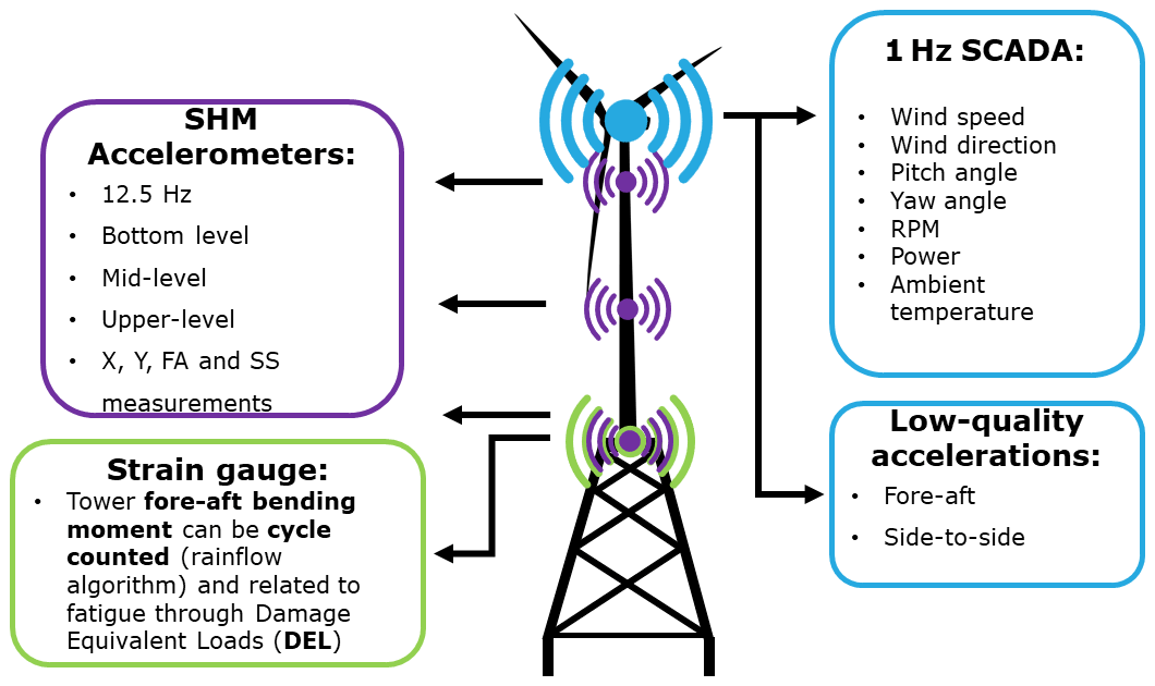
Figure 2 Overview of different sensors installed in wind turbine. Sensors locations are not accurate representations.

For this particular farm, SCADA data at a 1 Hz sample frequency were available for every turbine. The 1 s SCADA data contained, among others, wind speed (m s⁻¹), wind direction (^∘), pitch angle (^∘), yaw angle (^∘), rotational speed (cps, cycles per second), power (kW) and ambient temperature (^∘C). This wind farm also collected acceleration data from a built-in biaxial accelerometer in the nacelle on every turbine. However, this sensor was like the SCADA data sampled at a frequency of 1 Hz, and only the absolute value of the acceleration is stored.

In addition, data from two turbines with a full SHM setup were available. The SHM setup comprises three dedicated tower biaxial accelerometers with a sampling frequency of 12.5 Hz located at the tower bottom level, mid-level and top level. Apart from the accelerations in the two sensor directions, X and Y (with X in the dominant wind direction, often aligning with the fore–aft and Y 90^∘ from it), also the accelerations in the nacelle's frame of reference – i.e. fore–aft (FA) and side to side (SS) – are calculated through the use of the known yaw angle of the wind turbine. In addition, the collected SHM accelerations can also be transformed into displacements, through double integration in the frequency domain. To avoid excessive drifts in this transformation a lower frequency bound of 0.1 Hz is used (Maes et al., 2016).

These accelerometers outperform the accelerometers in the nacelle in three key properties. Firstly, the higher sampling frequency offers a wider frequency range. Secondly, they offered a much better signal-to-noise ratio than those installed in the nacelle. A third disadvantage of the nacelle accelerometer was that only the absolute values of this sensor were stored. A time series of the nacelle accelerometer is shown on top of one from the SHM system in Fig. 3.

Figure 3 Time series comparing the top-level FA SHM accelerometer signal and the nacelle-installed FA signal.

Alongside the accelerometers, the SHM setup also contains four axial strain gauges installed along the transition piece (TP) inner circumference at the TP–tower interface level. This setup of four strain gauges allows us to calculate the bending moments in both the FA (M_tn) and SS (M_tl) direction, when the yaw angle is known (Link and Weiland, 2014). For fatigue assessment the setup also cycle counts all strain and bending moment histories and calculates damage equivalent loads (DELs). After obtaining the bending moments, one can then employ a rainflow-counting algorithm (Dirlik, 1985) (reliant on a subset of the Python implementation of the WAFO toolbox; Brodtkorb et al., 2000), a well-known method widely discussed in literature (Marsh et al., 2016), which combines the number of cycles with their stress range. Finally, through the employment of a S–N curve (Ziegler and Muskulus, 2016) and Palmgren–Miner's rule (Kauzlarich, 1989), the damage equivalent loads are calculated. A more detailed discussion of this procedure can be found in Hübler et al. (2018).

Damage equivalent loads are usually presented under two forms: damage equivalent moments (DEMs) or damage equivalent stress ranges (DESs). These do not present two different quantities but rather two ways of presenting the same information – respectively as bending moments (Nm) or as stress MPa – easily translatable between one another using the moment of inertia. We can then understand the DEL as an umbrella term for both DEM and DES. The DEM is based on Eq. (1) as defined by Hendriks and Bulder (1995) (here presented for the stress ranges), wherein m is the slope of the S–N curve, n_i is the number of cycles of a given stress range (σ_i), r_o is the tower outer radius, r_i is the tower inner radius and N_eq=10⁷ is a predefined number of cycles. Following the discussion in Seidel et al. (2016), the compromise value of 4 was selected for m.

$$\begin{array}{}\text{(1)}& \mathrm{DEM}={\left({\displaystyle \frac{\sum _i{n}_i\cdot {\left(\frac{\mathrm{\Delta }{\mathit{\sigma }}_i\cdot \frac{\mathit{\pi }}{\mathrm{2}}\cdot \left(r_{\mathrm{o}}^{\mathrm{4}}-r_{\mathrm{i}}^{\mathrm{4}}\right)}{r_{\mathrm{i}}}\right)}^m}{N_{\mathrm{eq}}}}\right)}^{\mathrm{1}/m}\end{array}$$

As the DEL is a direct quantification of fatigue loads it can be considered as the primary input for any future fatigue assessment. But naturally these DEL values are only available for the two instrumented turbines. This paper aims to determine a methodology to estimate these DEL values for all turbines in the farm. In practice, this means that we can only rely on the SCADA data and the data from the nacelle accelerometer. In the current contribution we focus primarily on the DEL estimation in the FA direction, as measurements reveal it to be the most relevant for the current jacket foundations. However, the methodology equally applies for SS direction.

2.2 Methodology

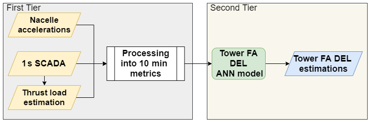
The main methodology of the present contribution can be understood as a two-tier neural network model. The first tier concerns itself with the generation and processing of relevant 10 min features, which will serve as inputs for the second tier. In the first tier, an ANN model is utilized to estimate the thrust load on a 1 s basis. This model has to be trained, validated and cross-validated before being considered fit for employment (upper white-background section of Fig. 4). After this, the 1 s thrust load, along with SCADA and accelerations from the SHM accelerometer, is processed into a variety of 10 min metrics (see grey section of Fig. 4). Between the 10 min feature generation tier (grey section of Fig. 4) and the DEL prediction tier (pale yellow section of Fig. 4), the 10 min metrics undergo a dimensionality reduction procedure based on a feature selection algorithm, which allows us to train, validate and cross-validate a 10 min ANN FA DEL estimation model for a fewer number of relevant input features. The motivation behind a 10 min approach lies with the common framework for data processing (also 10 min), the aim of including environmental effects and vibration levels, but also the issues inherent to working with different sampling frequencies (1 Hz SCADA, 12.5 Hz accelerometer) and possible time delays. After training, validating and cross-validating the DEL ANN model (middle white-background section of Fig. 4), we can observe this second tier in pale yellow in Fig. 4. Albeit the current contribution's methodology can be seen globally in Fig. 4, the sections which are under a white background consist of training, validation, cross-validation and determining which features ought to be used. Thus, these tasks will only be performed once. When a final model is achieved, only the sections with the grey and pale yellow background are required to produce estimations – this will be picked up again by Sect. 3.4.

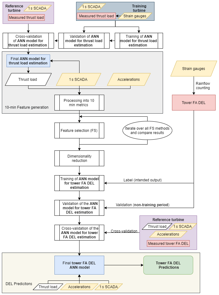
Figure 4 Flowchart representing the methodology's steps. Yellow highlights the sensors (and data by them captured), red the target, blue the final model and green the final results. Note that for ease of writing, as well as to differentiate from the ANN's thrust load predictions, the thrust load deduced from the strain gauges is mentioned as the measured thrust load.

2.2.1 Tier 1: 10 min feature generation

We can understand the first tier as globally contributing to generate and engineer relevant inputs (processed into 10 min metrics) for the model employed in the second tier. A particular element of the current implementation of this first tier is the prior training, validation and cross-validation, followed by the employment of a thrust load estimation neural network model based on high-frequency 1 s SCADA. The thrust load can be obtained from measurements by low-pass filtering the bending moment time series (with an upper frequency bound of 0.2 Hz; Noppe, 2019).

Historical research carried on the OWI-Lab by Noppe et al. (2018a, b) has shown the relevance the quasi-static thrust load assumes in the fatigue consumption in OWTs – albeit not being the sole contributor. It offers a direct insight into among others the role the controller can play in turbine fatigue life. Furthermore, the estimated load could potentially resolve the need for strain gauges through the use of thrust load estimation and acceleration measurements (Cosack, 2010; Baudisch, 2012).

The estimation of the thrust load is, in this contribution, performed through the use of an artificial neural network. This ANN was implemented using the tensor-manipulating framework TensorFlow, in particular its high-level API machine-learning library, Keras (Chollet, 2017), implemented on the programming language Python. The architecture selected for this ANN was a deep feed-forward neural network (Bishop, 2006). Research carried out by Schröder et al. (2018) into blade root flapwise damage equivalent load estimation has shown the greater performance of deep feed-forward ANNs when compared to other surrogate models, such as polynomial chaos expansion (PCE). This relative better performance should also be translated into tower bending moment DEL estimation.

In this contribution, feed-forward neural networks (Hastie et al., 2009) are employed using rectified linear activation functions, commonly referred to as ReLU (Glorot et al., 2011; Jarrett et al., 2009), a standard non-linear activation function for regression-focused feed-forward ANNs. The loss (the model's error) was calculated by a mean squared error loss function and is represented in Eqs. (2) and (3) for the DEL (D) and thrust load (F), respectively. Here, for a vector of n predictions, we have D_i or F_i, the vector of observed values, and $\widehat{{\mathit{D}}_i}$ or $\widehat{{\mathit{F}}_i}$, the vector of predicted values.

$$\begin{array}{}\text{(2)}& {\displaystyle }& {\displaystyle }\mathrm{MSE}={\displaystyle \frac{\mathrm{1}}{n}}\sum _{i=\mathrm{1}}^n{\left({\mathit{D}}_i-\widehat{{\mathit{D}}_i}\right)}^{\mathrm{2}}\text{(3)}& {\displaystyle }& {\displaystyle }\mathrm{MSE}={\displaystyle \frac{\mathrm{1}}{n}}\sum _{i=\mathrm{1}}^n{\left({\mathit{F}}_i-\widehat{{\mathit{F}}_i}\right)}^{\mathrm{2}}\end{array}$$

In order to minimize the loss function, an optimizer is required during the ANNs training. A common, well-performing choice is the adaptive moment estimation algorithm, also known as Adam, or, in this particular case, Adamax, an extension of Adam based on the infinity norm (Kingma and Ba, 2014). This particular optimizer was selected through hyperparameter tuning by comparison with other available optimizers, such as stochastic gradient descent (SGD), root mean squared propagation (RMSProp) and Adadelta (Zeiler, 2012), an extension of the adaptive gradient algorithm, Adagrad.

As mentioned, the ANNs' training will proceed until a given number of epochs is reached. A threshold of 100 was defined, as initial sensitivity analyses showed the model converging to a solution well before 100 epochs. This performance was monitored through the mean absolute error and root mean square error of the training and validation datasets (i.e. an independent dataset not used during training). In order to prevent the model overfitting for the training dataset, an early stop callback mechanism with a patience of 10 epochs was implemented (Prechelt, 1998; Caruana et al., 2001).

The final thrust load estimation ANN topology had four hidden dense layers – i.e. four intermediary layers between the input and output layers where every neuron is connected to every other neuron in the next layer – with a varying number of neurons (from 64 to 300), achieved through hyperparameter tuning.

The thrust load, along with the SCADA and acceleration data, is then processed into 10 min metrics. These include widely known statistics as mean, minimum, maximum, median, mode (most common repeated value), standard deviation, range and root mean square (rms) computed from 10 min intervals of the time series. In addition also more atypical statistics such as spectral moments (first to fourth, Miller and Rochwarger, 1970; Grimmett and Stirzaker, 2020), skewness and kurtosis are calculated from the time series. The selection of which engineering input features should be calculated can be traced to Vera-Tudela and Kühn (2014). The formulae for these metrics can be found in Table A1. Apart from these statistical metrics, metrics that are rooted in fatigue assessment are also included. In particular, the damage equivalent moment (DEM) of the estimated thrust load is calculated, in a way representing the fatigue contribution of only the thrust load. In addition the damage equivalent acceleration is calculated by first cycle counting the SHM accelerations – both the original signals and the signal “transformed” into displacement. We can see them in Eq. (4), where a(t) stands for the acceleration signal. The damage equivalent accelerations (DEAs) do not have any immediate physical meaning in terms of fatigue but could be interpreted as a fatigue-weighed mean amplitude of the acceleration.

$$\begin{array}{}\text{(4)}& \mathrm{DEA}={\left({\displaystyle \frac{\sum _i{n}_i\cdot \mathrm{\Delta }a(t{)}^m}{N_{\mathrm{eq}}}}\right)}^{\mathrm{1}/m}\end{array}$$

The transformation of the original acceleration signals into displacements is performed through double integration in the frequency domain, as shown by Eq. (5). Here, ℒ stands for the Laplace transformation, a(t) stands for the acceleration signal, s stands for the circular frequency (2π×f) and x(t) stands for the transformed displacement signal. This transformation is discussed in depth in Maes et al. (2018).

$$\begin{array}{}\text{(5)}& x\left(t\right)={\mathcal{L}}^{-\mathrm{1}}\left\{{\displaystyle \frac{\mathrm{1}}{s^{\mathrm{2}}}}\mathcal{L}\mathit{\left\{}a\right(t\left)\mathit{\right\}}\right\}\end{array}$$

After the processing of all high-frequency signals (35) into 10 min metrics, a total of 430 metrics is available for each 10 min interval. Given the large number of variables, some dimensionality reduction prior to the second tier of the algorithm is desirable.

2.2.2 Feature selection

Feature selection encompasses a number of methods focused in reducing the number of input variables of predictive models into the variables believed to be the most useful to the models (Leray and Gallinari, 1999). The reduction of input variables is frequently desirable as, by removing redundant variables, computational, memory and time costs are reduced (Guyon and Elisseeff, 2003). Moreover, it has been shown that dimensionality reduction may improve the overall performance of neural network models, as non-informative variables can add uncertainty to the predictions and reduce the overall effectiveness of the model (Kuhn and Johnson, 2013). ANN models' performance is thus highly dependent on the input data's quality, with certain inputs being vastly more relevant than others for the model's performance (Schröder et al., 2020).

Apart from enabling a dimensionality reduction, feature selection can also help identify the most important input parameters. Knowing which features are relevant can be valuable information in assessing the added value of certain sensors, here in particular the accelerometers, required signals from SCADA and the metrics that are worth calculating. As such, the outcome of the feature selection may offer the possibility to optimize setups and reduce the number of SCADA data that have to be made available by the operator and processed.

Feature selection methods can be classified and grouped into various categories. Firstly, one can distinguish between supervised and unsupervised methods: if the outcome is not ignored (i.e. we have a target variable), then the technique is supervised. This is precisely the case of the present contribution, wherein the target variable is the DEL of the tower FA bending moment. Thus this contribution will solely focus on these methods. Supervised feature selection algorithms can be further subdivided into intrinsic, wrapper and filter methods.

Starting with the filter-based feature selection methods, these employ statistical techniques to evaluate the relationship between each input variable and the target variable, assigning a score for the relevance of the input variable. The scores obtained for the relationship between the variable and the target are then used to choose (filter) the inputs that will be used in the model. Filter-based feature selection methods include Pearson's r, dominance analysis, Spearman's ρ, Kendall's τ and K-best. These were computed using the Python packages scipy.stats, dominance_analysis and scikit-learn.

Differently, wrapper feature selection methods generate several machine-learning models evaluating different subsets of input variables, wherein the selected features are the ones that are present in the model that performs better, according to a performance metric, such as the mean squared error (MSE), used in this paper. These methods' models use processes that add/remove predictors until an optimal combination that maximizes model performance is found. Unlike filter approaches, wrapper methods are able to detect the possible interactions between variables. There are, however, disadvantages, such as an increasing overfitting risk (for small samples) and a very significant computation time if the number of variables is large. Wrapper feature selection methods include recursive feature elimination (RFE), in which a machine-learning algorithm present in the core of the model is fitted, the features ranked by importance, the least relevant features iteratively discarded and the model then re-fitted, with the processes being repeated until the required number of features is achieved. In this contribution, the machine-learning algorithms used in the core of the RFE, also known as estimators, were a random forest (RF) regressor and a decision tree classifier (DTC).

Finally, intrinsic methods represent feature selection models which possess built-in feature selection. This means that the model only includes features that maximize the accuracy, thus performing automatically a feature selection during training. These include penalized regression models and decision trees, such as random forest algorithms which are an ensemble of decision tree algorithms that generate several decision trees during training and output the mean/average prediction of the individual trees. A deeper look into these methods can be seen in d N Santos et al. (2020b).

One final word should also be added regarding the popular methods principal component analysis (PCA, Jolliffe and Cadima, 2016) and neighbourhood component analysis (NCA, Goldberger et al., 2004) and their non-inclusion in the present contribution. Although certainly powerful dimensionality reduction tools, both PCA and NCA are unable to provide insights into the original variables, as they transform the variable space (into principal components). It was deemed interesting to just work with the pre-existing variables, as they are related to the installed sensors, and one can then learn more about their relative importance. This knowledge would not be possible if PCA or NCA were to be employed.

2.2.3 Tier 2: estimation of DEL using an artificial neural network

The second tier of the current contribution's model uses the features engineered in the first tier that were picked up during the feature selection process as input. The measured tower bending moment DEL, attained from the strain gauges, is used as the label, or intended output, during the training stage of the ANN model, prior to its employment in the second tier (see middle white-background section of Fig. 4).

Much like with the ANN used to estimate the thrust load, the tower bending moment DEL feed-forward ANN model is implemented on Python through the machine-learning library Keras – based on the tensor-manipulation framework TensorFlow. The activation functions between each neuron were, once again, rectified linear transfer functions and the loss function MSE. The use of MSE as a loss function is particularly important in this application as MSE is more sensitive to outliers than other loss functions, which is relevant as the DEL is very sensitive to higher loads (Liano, 1996). For this particular application, it was found, through hyperparameter tuning and monitoring of the MSE, that the Adam optimizer was the best-performing optimization algorithm. The final topology of the tower bending moment DEL ANN presented six dense hidden layers with 18–500 neurons.

After training, this model was validated on the same year as the training year (excluding the training period) and a different year, as well as cross-validated on the other fully instrumented turbine for a whole year before being employed (pale yellow section of Fig. 4).

3 Results and discussion

3.1 Thrust load model

Following the methodology prescribed in the previous section, one must first exhibit the results for the training, validating and cross-validating of the artificial neural network that estimates the thrust load. The full results and discussion can be found in d N Santos et al. (2020a). The high-frequency SCADA data used to train consisted in wind speed (m s⁻¹), rotor speed (cps), mean pitch (^∘), nacelle orientation (^∘) and actual active power (kW) from 12 d, carefully selected as to be statistically representative of all operating conditions, namely parked, run-up and full load. Strain measurements from the same time period undergo a temperature compensation before calculating the resulting bending moments and filtering this last signal with a low pass filter with an upper frequency bound of 0.2 Hz. The filtered FA bending moment M_tn signal is subsequently translated into thrust load, which must further be corrected for the air density (Baudisch, 2012; Noppe et al., 2018b).

The model training, monitored through the mean absolute error (MAE) and root mean square error (RMSE), was deemed satisfactory, as convergence was achieved with both MAE and RMSE below 1 %. We can observe the model's output when plotting a discrete time series of interest, e.g. when the turbine is operating at rated power (see Fig. 5), and we compare the predictions with the measured values of the thrust load. In this figure, we can observe how close the predictions accompany the measured thrust load, capturing almost fully the base quasi-static loading behaviour.

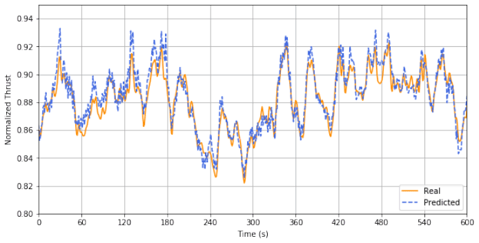
Figure 5 Measured (orange) and predicted (blue) thrust values for a 10 min time instance at rated power.

The model was then validated for 3 months of data outside of the training period on the same turbine as for training. The model was also applied to a different (non-training) wind turbine with a similar SHM setup, the cross-validation stage. The results for predicted thrust load were compared with the measured values attained from the strain gauges at this location. This cross-validation served to assess whether the model is transferable to other turbines in the farm. In Fig. 6 we can observe the model's performance (through the mean absolute error expressed as a percentage of the maximal thrust load value) for both the validation and cross-validation datasets plotted against the wind speed (MAE binned according to the wind speed with a step of 2 m s⁻¹).

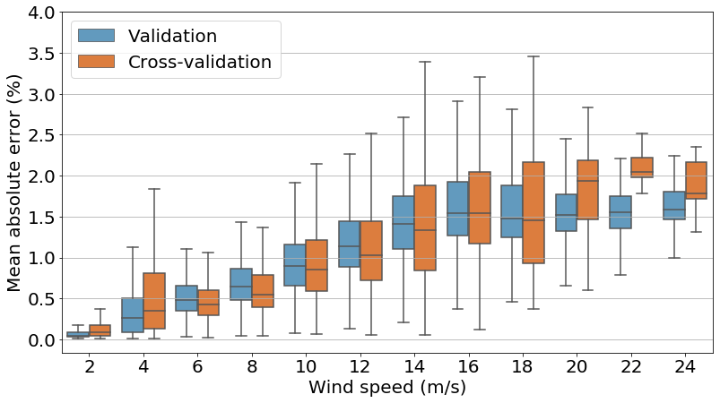
Figure 6 Box plot of MAE of thrust load estimations, expressed as a percentage of the maximal training thrust load value (binned) for the validation and cross-validation turbines plotted against wind speed.

For both cases (validation and cross-validation) we can observe that both curves are rather similar, with one and the other presenting a slight increase in the MAE as the wind speed increases and most values staying below 2 %. The increase in MAE with the wind speed is expected, as higher loads are attained for higher wind speeds (and the MAE relates to the absolute value of the loads). The two curves differ in the fact that, for the cross-validation, the MAE box plots present slightly larger whiskers. A small number (3) of overshoots prior to a rotor stop, not present in the training dataset, and whose cause remains undetermined were also identified for the cross-validation. We can understand the higher maximal value for the cross-validation (attained for 4 m s⁻¹) as being related to these overshoots prior to a rotor stop.

Regardless of the presence of these overshoots, they do not overly influence the final results, as both the original and cross-validation turbines' MAE box plots remain highly similar. This similitude allows us to affirm the transferable nature of the ANN model to other offshore wind turbines.

3.2 Parameter and sensor significance

A key concern of the current contribution is to understand the added value each sensor brings to the predictive model, in particular, the contribution of the dedicated tower SHM accelerometer. Apart from enabling us to reduce the input variable space's dimensionality, the performance of a feature selection routine also allows us to identify the most important parameters engineered in the first tier (see Sect. 2.2.1 and 2.2.2) and linking them with the original sensor, which in turn allows us to assess whether a particular sensor is worth adding to the setup.

Finally, in order to assess the gains the current instrumentation layout presents relative to less-instrumented turbine setups, a comparative analysis based on ANNs is carried out for eight different instrumentation scenarios.

3.2.1 Feature selection

As mentioned above, in order to understand which engineered features are relevant to determine the tower bending moment DEL (and thus, which sensors are important), several feature selection algorithms are studied and the groups of features they select registered. Before performing any feature selection routine, one must first engineer the necessary 10 min features.

The thrust load, accurately estimated as detailed in Sect. 3.1, can then be, along with the acceleration and SCADA signals (in a total of 35 high-frequency parameters), processed into 10 min metrics, as seen in Sect. 2.2.1. The different permutations between signals and metrics generate a total of 430 features available at 10 min intervals.

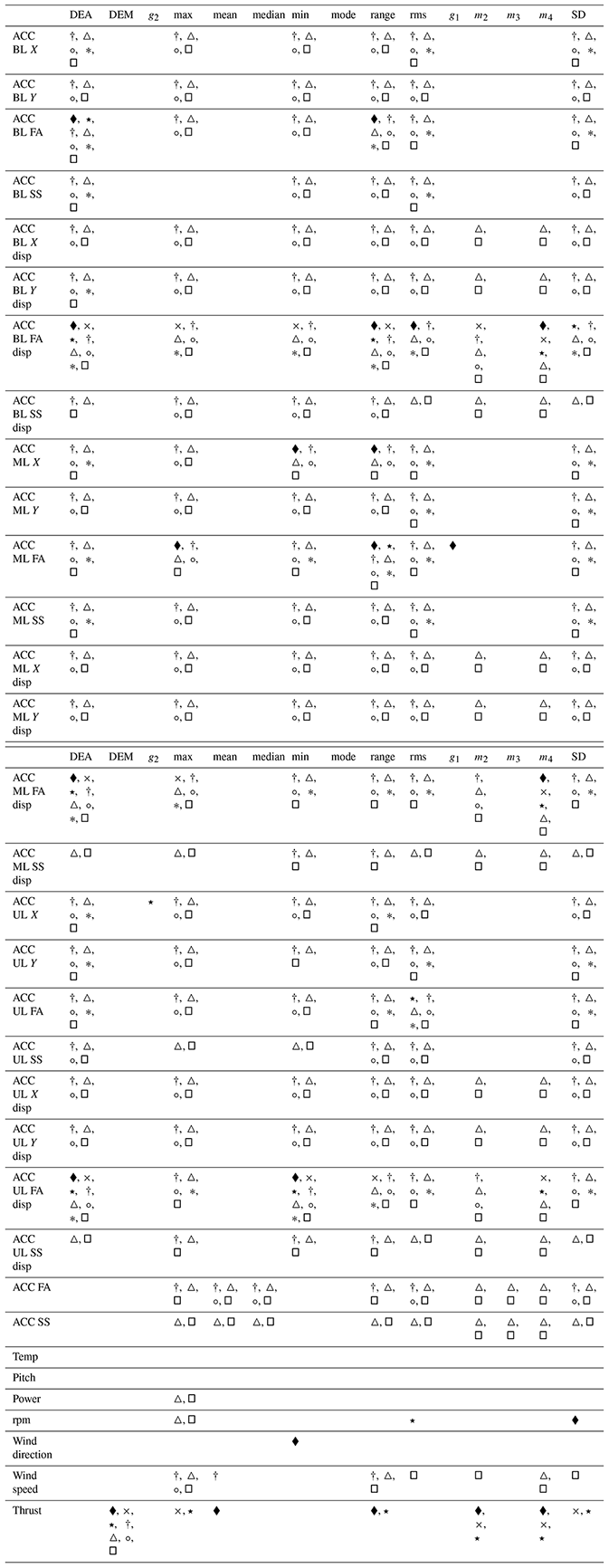
This large number of features further elicits the need to perform a feature selection study, in order to lead to a reduction in the number of the input variables. Several methods were compared, including filter-based methods (Pearson's r, dominance analysis, Spearman's ρ, Kendall's τ, K-best), wrapper-based methods (recursive feature elimination (RFE) with either a decision tree classifier or a random forest estimator – feature ranking algorithm) and an intrinsic method (random forest), described in Sect. 2.2.2. In Table 1 we can observe each feature selection method, along with the number of features (also expressed as a percentage of total number of features) selected by each method and the class. The full results of the feature selection are shown in Appendix B in Table B2. Table B1 provides a quick explanation of the nomenclature employed. A more in-depth discussion can be found in d N Santos et al. (2020b).

Table 1 Feature selection methods, classes and number of features selected.

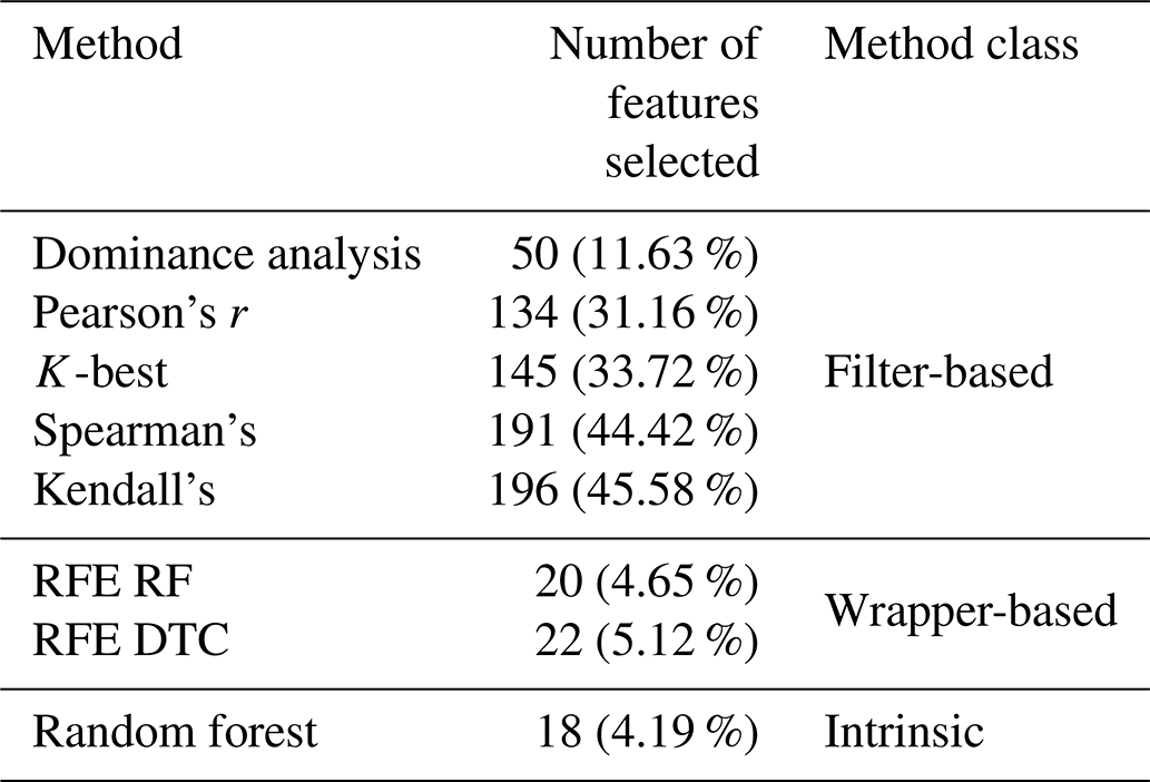
Table 1 shows a clear distinction between filter-based and other methods, wherein the former selects 100+ features. This might be because filter-based methods are not non-linear, which might increase the difficulty in discerning the most important features and effectively withholding non-relevant ones. Nevertheless, to properly assess the performance of each feature selection method, the features selected by each feature selection method were fed into a generic feed-forward artificial neural network. The ANN presents two hidden layers with 50 and 100 neurons, respectively, using a rectified linear activation function between each layer. The number of neurons in the input layer is equal to the number of features selected by the feature selection method. The ANN also applies an Adamax optimizer and a mean squared error loss function with the target being the tower FA bending moment DEL, as well as a limit of 100 epochs. The training–testing split was performed through k-fold cross-validation with 10 folds and a batch size of five, which allows us to assess the generalization of each model (Anguita et al., 2012). The results for each method are presented in Fig. 7. The spread in results for each method is due to the 10-fold cross-validation, and methods' classes are distinguishable through a colour scheme: green (intrinsic), orange (wrapper) and blue (filter).

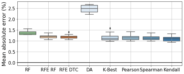
Figure 7 Mean absolute error of every feature selection method's ANNs as a percentage of the maximal DEL value. RFE stands for recursive feature elimination, RF for random forest, DTC for decision tree classifier and DA for dominance analysis.

In Fig. 7, we can observe that all methods present similar values (between 1.5 % and 1 %), apart from dominance analysis. Upon first glance, one would be tempted to assume that Kendall's τ is the best model, as it presents a marginally lower mean MAE than other methods. However, it is also crucial to look at the number of features selected by each model (see Table 1). The intrinsic and wrapper methods selected around 20 features, whereas filter-based methods (apart from dominance analysis, which selects 50 features) all selected above 100 features. For the latter, the higher the number of features, the better the model's performance. This evidenced by Fig. 8.

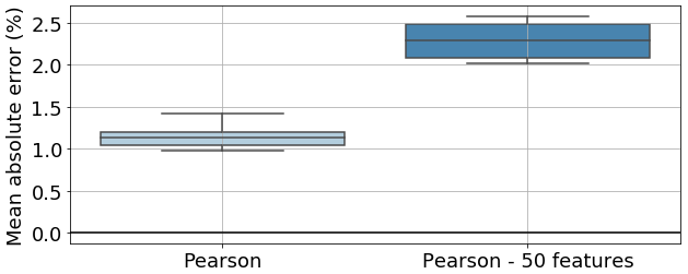
Figure 8 Comparison of mean absolute error between model trained with features selected by Pearson's r and just the first 50 features selected.

In Fig. 8 we can see that, for Pearson's r, if, instead of 134 (31.16 % of the total number of features) features selected, there are only 50 (11.63 %) features selected, the MAE increases by over 1 % (attaining a similar value to dominance analysis).

Given the results shown in Fig. 7, we are then in the presence of a trade-off scenario: either we have a small number of highly relevant features selected by recursive feature elimination, and thus, a high computational cost in feature selection but smaller cost in neural network model training and input variable processing, or we have a high number of features selected by filter-based methods, which entails a small computational cost for feature selection and a bigger cost for neural network model training.

Naturally, as the objectives of Sect. 3.2 are to reduce the dimensionality of the input variable space and gain insights into the most important features (and therefore the most important sensors), filter-based feature selection methods ought to be discarded in favour of intrinsic or wrapper methods. These latter, for a low number of features (around 20), present models which perform as well as models involving higher numbers of features.

If we now focus on wrapper methods (see Table B2), we notice that these select solely FA and X acceleration/displacement signals, whilst also selecting rpm, thrust and wind direction. These methods pick up metrics such as kurtosis and skewness but also DEA, DEM, rms, range, SD, maximum, minimum, mean, and the second and fourth spectral moments. As for intrinsic methods, they only selected metrics for bottom level, mid-level and upper-level FA displacements (DEA, maximum, minimum, range, and second and fourth spectral moments) and for thrust (DEM, maximum, SD, and second and fourth spectral moments).

Globally, we can say that some metrics are selected more often by all methods – DEA, rms, range, minimum, maximum and SD – and that some features are selected by all methods – DEA of FA displacement for bottom level, mid-level and upper level, range of FA bottom-level displacement, minimum of FA upper-level displacement, and DEM of thrust.

The fact that all methods select DEA FA displacement metrics and the DEM of thrust is understandable, as this was the initial assumption behind the cycle counting of these signals – that they would more closely relate with the target, the tower FA bending moment cycle-counted DEL. Likewise, the more often selected statistics (rms, range, SD, minimum, maximum) relate to variations within the signal, which is the most relevant in the cycle-counting process.

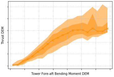
When focusing on SCADA-related features, we can observe that wrapper (RFE) and intrinsic methods select SCADA-related metrics which were not picked up by filter methods – mean, maximum, range, SD, and second and fourth spectral moments of thrust but also SD and rms of rpm and minimum wind direction. The higher number of thrust-related metrics selected might be due to its initially linear relationship to the tower FA bending moment DEM (see Fig. 9, where especially for lower wind speeds there's a linear correlation). SCADA parameters such as the wind direction are only picked up by the wrapper methods. These, along with the intrinsic method, also signal the spectral moments more. Again, this is to be expected, as filter-based methods, even nonlinear ones such as Spearman (dependent on monotonic functions) and Kendall, cannot pick up the more complex interactions between the SCADA data and the target variable. Only two parameters were not chosen by any feature selection algorithm – the temperature and pitch. Nevertheless, if we discard filter-based methods, SS and Y SHM accelerations appear to be unnecessary for this site, along with the low-quality nacelle-installed absolute accelerations, power and wind speed. Likewise, only three metrics were not select by any method – median, mode and the third spectral moment; in future uses of this methodology, these need not be considered.

Figure 9 Thrust DEM vs. tower fore–aft bending moment DEM.

In sum, the more trustworthy wrapper and intrinsic methods give us then more meaningful features; this has lead to the selection of RFE (DTC) for further use (in Sects. 3.2.2 and 3.3), instead of RF or RFE RF, as it presented a better, albeit marginally so, performance. We can also clearly affirm that one ought to engineer a varied set of features (including spectral moments, kurtosis, skewness, rms and cycle counting the signal) stemming from the SHM accelerometers (for FA and X direction signals, which should also be translated into displacement) and the thrust load estimation (with a desirable inclusion of certain SCADA-related features, such as wind direction and rpm). It ought to be reinforced that the conversion of SHM accelerations to displacements appears to be crucial. Metrics such as median, mode and the third spectral moment seem to bear no fruits, as do the Y and SS SHM accelerations, low-quality nacelle-installed absolute accelerations, temperature and pitch. The SHM acceleration parameter with most metrics selected was the FA bottom-level displacement signal, which might mean that this is the most important placement for the accelerations – a surprising result as it was expected that the top side accelerometer would be a better placement. Nevertheless, in order to identify the most important placement of the SHM accelerometer (if at bottom level, mid-level or upper level), it would be desirable to perform a dedicated study with three scenarios – with only one SHM accelerometer at a level per scenario. This has to, for the time being, be left for future research tasks (especially for monopile foundations).

In this section, several feature selection methods were compared, with a clear preference for wrapper or intrinsic methods, and the relevant metrics and sensors (and signals) identified, with it being then apparent that, when faced with an instrumentation scenario as described in Sect. 2.1, nacelle-installed low-quality accelerometers should be disregarded in favour of SHM accelerometers, the calculation of FA and (to a lesser extent) X displacement metrics should be prioritized over SS and Y, and that the estimation of thrust load is paramount. The authors would like to point out that the conclusions related to which features are to be selected are connected with the site at question and that it is a good practice to redo feature selection for a different site.

Table 2 Scenarios investigated. Different scenarios imply that different data sources are considered to be available, in line with real-world experience. For example, scenario A considers that only 10 min statistics of SCADA are available, while scenario H covers a near-ideal situation only possible on the two SHM turbines. Scenarios D and F are possible at all turbines of the particular farm in this contribution. Note that the access to 1 s SCADA inherently implies access to 10 min SCADA. Some scenarios exclude the calculation of the 1 s thrust load estimation to assess the added value of calculating this type of parameter.

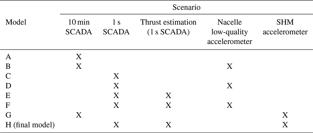
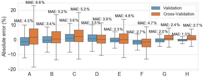
Figure 10 Comparison of the ANN model's performance in validation and cross-validation for eight different sensor data quality scenarios. Error expressed as a percentage of the absolute maximal training DEL value.

3.2.2 Minimal instrumentation study

In the previous section we have seen how the most valuable sensors are the dedicated tower SHM accelerometers, along with the estimation of the thrust load based on 1 s SCADA, and which metrics are more relevant. However, in order to fully answer what is gained with the addition of each sensor and by their increased quality, an additional analysis is required. This is particularly relevant, as the instrumentation setup described in Sect. 2.1 is not always present or even the most commonly present in wind farms.

To this point, eight different plausible scenarios are defined. Each scenario only considers a subset of all parameters to be available, in line with scenarios OWI-Lab has experienced in past projects (scenarios involving 10 min SCADA and low-quality nacelle absolute accelerations are typical for older wind turbines, whereas the inclusion of 1 s SCADA and/or SHM accelerometers is sometimes seen in newer turbines). These scenarios are identified in Table 2. For each scenario a model is trained and is tested for a validation and a cross-validation dataset, both comprising in total of 1 year worth of data. The validation dataset is comprised of the dataset of the year of the ANN training, and the cross-validation is comprised of a dataset of 1 year of another non-training turbine. Both results are presented together, in which the cross-validation results allow us to assess to what level the results can be transferred from one turbine to another.

Scenario H, the final model, follows the methodology prescribed in Fig. 4 and, as presented in Sect. 3.2.1, uses the data selected using the RFE DTC feature selection algorithm (the only scenario where feature selection was performed), including components from 1 s SCADA, dedicated tower SHM accelerometers and the thrust load. The RFE DTC was the chosen method, as explained in the previous section. Scenarios D and F – 1 s SCADA, low-quality nacelle absolute accelerations and thrust load in the case of F – are the prevailing instrumentation scenarios throughout the farm in this contribution, except for the two aforementioned fully instrumented turbines (scenario H), and will be further discussed in Sect. 3.4.

In Fig. 10, we can see the absolute error box plots, expressed as a percentage of the maximal training dataset DEL, with the MAE also indicated. Here, the absolute error relates to the absolute values, and not the modulus, and is given by the difference between real and predicted values, $X_i-\widehat{X_i}$ (presented as a percentage of the maximal DEL).

Some general remarks can be drawn by analysing this figure. Firstly, when comparing the first four scenarios (A–D), we can see that the inclusion of 1 s SCADA induces a better model, with a lower MAE (specifically if we consider the cross-validation). Both for 10 min SCADA and for 1 s SCADA the inclusion of nacelle-installed low-quality accelerometers (B and D) does not necessarily enhance the performance of the model itself (validation MAE, in blue, does not improve that much, especially for 1 s SCADA), but it does improve the model's generalization to other turbines (cross-validation MAE, in orange, almost decreasing by 2 % for both cases). We can try to understand this as implying that, albeit for a single turbine SCADA data alone might provide a decent enough model, if we want to apply a model to different turbines, then the inclusion of accelerations is paramount.

Focusing on 1 s SCADA, we can see that the inclusion of the thrust load (E and F) further improved the model itself (validation) but is not able to generalize as well for the cross-validation turbine, actually slightly degrading the results when compared to 1 s SCADA and nacelle-installed accelerations (D), suggesting that the thrust load model was overfitted to the training turbine. Such an issue could be potentially resolved when considering multiple turbines for the training of the thrust load model. However, with only two instrumented turbines, in which the second turbine serves as a cross-validation, it was opted to only consider data from the single training turbine.

Pivoting back to 10 min SCADA, if we include dedicated tower SHM accelerometers (G), again we see accelerations improving the generalization but this time also vastly improving the model performance (MAE close to 2 %, error well between the minus and plus 10 % bounds). This might be due to the fact that, with more accurate accelerometers, with greater quality, a fuller picture of the structural dynamics can be drawn for both the validation (training) and cross-validation turbines. Scenario G – 10 min SCADA and SHM accelerations – should also be highlighted, as it performs rather well (both MAEs around 2 %). This is especially relevant for older wind farms, where usually 1 s SCADA is not available. Finally, the results for the model based on the RFE DTC selected features are the best for the turbine (H), as they have the lowest MAE and smallest inter-quartile range for the validation turbine.

We can then say that the best models include data from SHM accelerometers and are able to present MAEs of around 2 %. The 1 s SCADA models can have their performance enhanced by estimating the thrust load (however, concerns regarding the adaptability to other turbines should not be ignored) or by including nacelle accelerations. These models had MAEs of around 4 % for cross-validation, with most errors falling within ±10 %. For just 1 s SCADA or 10 min SCADA models (A, B, C), MAEs are above 5 % and most cases will fall within ±20 %. It is up to the operator, then, to determine which bounds are considered acceptable.

The present contribution provides a detailed overview of how the ANN-based methodology might perform for different instrumentation scenarios on jacket-foundation offshore wind turbines. It is expected that, for monopile-foundation OWTs, where the importance of wave-related dynamics is much greater, other conclusions will be drawn as to the minimal instrumentation setup performance.

3.3 Fatigue rate (DEL) estimation

Following the discussion held in the preceding section (Sect. 3.2), a deeper look into the best-performing model – scenario H – is performed.

For this, several ANN topologies were tested employing the Adam optimizer and a mean squared error loss function, a limit of 100 epochs, k-fold cross-validation with 10 folds, a batch size of five, and monitoring of MSE and RMSE. Of the different tested topologies, the best-performing one presented five hidden layers with 100, 200, 300, 200 and 100 neurons, respectively. The data selected for training consisted in a randomized sample of 8000 non-consecutive data points within a given year (the training dataset represented 35.7 % of the available data for that one year, with a random 80 %–20 % train–test split). The deep neural network was then trained on this dataset, its performance was tested on the testing dataset, and it was then validated on a different period in the same year outside the training period, a different year, and cross-validated for an entirely different turbine. The training turbine is located at the northwestern edge of the farm, and the cross-validation turbine is located in the middle of the farm (see Sect. 3.4, OWT 7 and OWT 35 of Fig. 16). In Fig. 11 we can see plots of the time series for normalized DEL (both for the validation and cross-validation datasets) for a period of 7 d. We can see how, for both cases, the predictions closely accompany the measured behaviour.

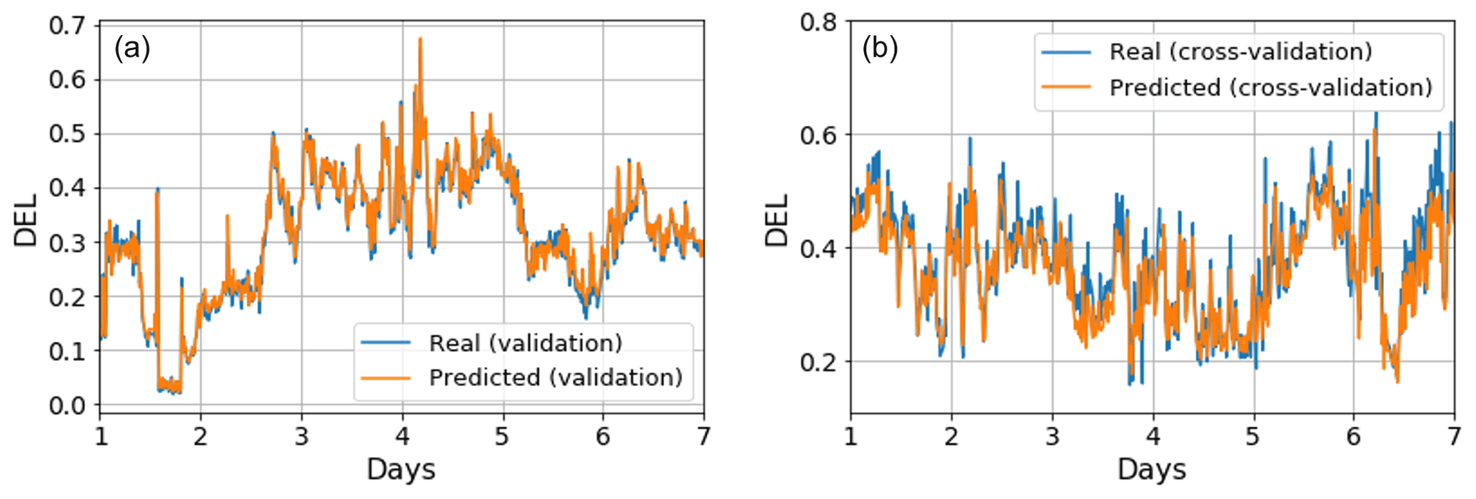
Figure 11 (a) Time series of DEL for 7 d of the validation dataset (real – blue; predicted – orange). (b) As in panel (a) but for the cross-validation dataset (different turbine from training).

In Fig. 12, the absolute error of the tower FA bending moment DEL predictions, estimated as for Fig. 10, expressed as a percentage of maximal value of DEL (for training) is plotted for the training year, a different year (but still in the training turbine) and a different turbine. Additionally, the MAE for each case (also expressed as a percentage of the maximal training DEL), is superimposed on the plot.

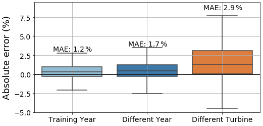
Figure 12 DEL prediction error for validation (training year and different year) and cross-validation, expressed as a percentage of the maximal DEL. Error expressed as a percentage of the absolute maximal training DEL value.

Here we can see that the model performs rather well for the training year – the MAE is kept around 1 %. Likewise, for a different year, the model performs rather well, with a MAE of 1.7 %, although a slight underprediction is noticeable (a positive error means that the real value is superior to the prediction, also existent for the training year) and there is a marginally bigger spread. Nevertheless, differences for the performance between the training year and different year are almost negligible. The model then seems to properly adapt and generalize. We can thus conclude that the model performs appropriately, presenting sufficient generalization to successfully predict for datasets which do not correspond to its training period, with a MAE around 1 %, which is within the bounds defined established Sect. 3.2.1.

Things, however, change for a different turbine: the MAE increases about 2-fold to 2.9 %, the spread for the error is much more noticeable and there is an accentuated underprediction (positive error). There may exist several, non-exclusive, reasons behind this degradation of the model's performance for a different turbine – located in the turbines' wake – than that of training. Firstly, one cannot ignore the inherent site dependency of the trained model: the ANN was trained on a given turbine, so it is expected that, even though it is able to capture the overall behaviour of other turbines of the same farm, it will have a greater difficulty to adapt to different turbines as well as for the training turbine. Additionally, as seen in Sect. 3.2, the inclusion of thrust-related metrics might further enhance site dependency. Furthermore, this site dependency can be increased by the feature selection process – the features that are selected are for the training turbine; these might possibly differ for the cross-validation turbine. One possible way to circumvent this would be to have a population-based model (Antoniadou et al., 2015; Worden et al., 2020) which would use the data of both turbines during training. However, for our current study, this would impede the cross-validation as only two turbines are available. Nevertheless, we can still affirm that, albeit the relatively worse results for cross-validation (different turbine), the model still performs within the realms of acceptability, giving us a certain degree of trustworthiness.

In Fig. 13, we can take a deeper look at the model's performance, wherein in Fig. 13a the absolute error of the tower FA bending moment DEL predictions is binned according to the wind speed with a step of 2 m s⁻¹ for the validation dataset (year of training) and the cross-validation dataset (different turbine).

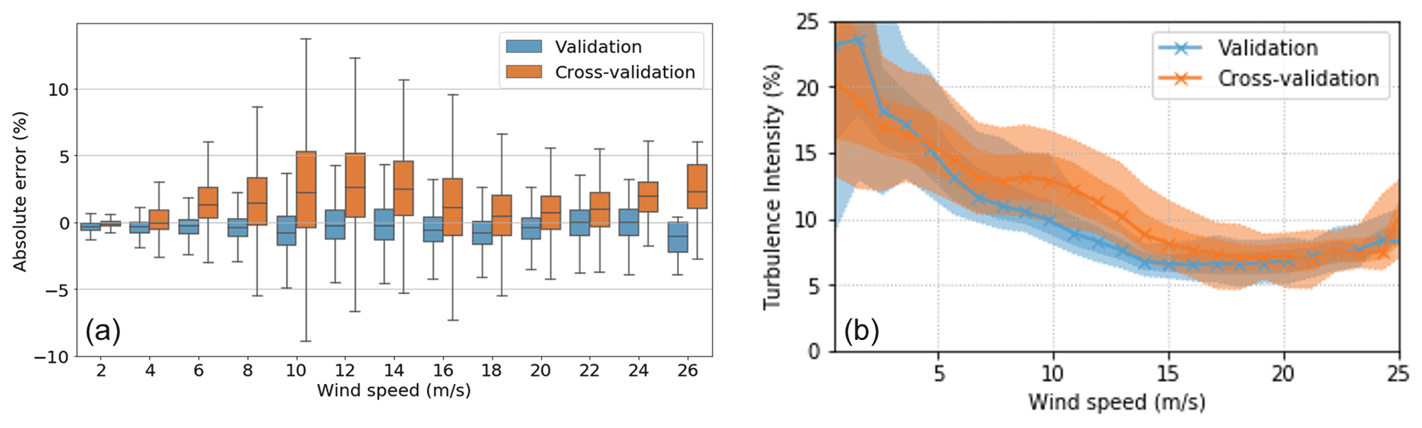
Figure 13 (a) Box plot of error expressed as a percentage of the absolute maximal training DEL value (binned) for the validation and cross-validation turbines plotted against wind speed. (b) Turbulence intensity (%) vs. wind speed (m s⁻¹) for validation and cross-validation turbines.

Here, we can verify the better performance of the model for the validation dataset, as evidenced by Fig. 12, and that the model is underpredicting for the different turbine (cross-validation). More interestingly, we can observe how the model performs worse for a different turbine for mid-range speeds (8–18 m s⁻¹) rather than for higher speeds. This is possibly related to the worse performance of the model under wake. Avendaño-Valencia et al. (2021) worked in this direction, concluding that the fatigue life of OWTs under free-stream inflow can be quite distinct from OWTs under wake (Avendaño-Valencia et al., 2021). This can be further verified by inspecting Fig. 13b, where the turbulence intensity is plotted against the wind speed, as turbulence intensity (TI) is given by $\mathrm{TI}\left(\mathit{\%}\right)=\left(\mathit{\sigma }\right(u)/\stackrel{\mathrm{‾}}{u})\times \mathrm{100}$, where σ(u) represents the standard deviation of wind speed and $\stackrel{\mathrm{‾}}{u}$ the mean wind speed. The values of turbulence intensity for lower wind speeds are rather unstable and thus disregarded in this analysis. In this figure we can see how, for wind speeds between 5 and 18 m s⁻¹, the turbulence intensity of the cross-validation turbine is noticeably higher than for the validation (and training) turbine. We can then reasonably assume that, precisely because the cross-validation turbine faces higher turbulence (being located under more severe wake) than the training turbine, the prediction error for the cross-validation turbine will be highest in the regions where the gap between turbulence intensities is greater.

Additionally, in Fig. 14 we can observe how, even for the training turbine (OWT 7; see Sect. 3.4), a similarly higher error appears for the training turbine when operating under wake. Even though the number of data is noticeably lower (thus, there are only box plots up to 18 m s⁻¹), we can also see the higher errors above 10 m s⁻¹.

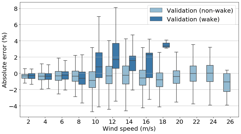
Figure 14 Box plot of error expressed as a percentage of the absolute maximal training DEL value (binned) of DEL for the validation/training turbines plotted against wind speed under wake and under free-flow conditions.

This worse performance for the cross-validation might be possibly due to a lack of under-wake data and could be enhanced through wake transfer models or a population-based approach. Nevertheless, we can say that, overall, the tower bending moment FA DEL ANN model performs well and presents itself as a viable solution for DEL estimation under a fleet-leader concept.

3.4 Farm-wide

In this final section the proposed methodology is used in a real-world farm-wide setting with 48 assets. Figure 15 schematizes the pipeline for the farm-wide model, consisting in the parts of Fig. 4 which are kept for producing DEL estimations – the 10 min feature generation and DEL predictions tiers, in grey and pale yellow, respectively.

Figure 15 Schematic of tower FA DEL estimation ANN methodology.

As mentioned in Sect. 3.2, most turbines present in the wind farm do not possess fully instrumented setups (scenario H; see Table 2) but rather 1 s SCADA (which allows us to obtain the thrust load) and low-quality nacelle-installed accelerometers. According to Fig. 10 the best-performing model in this scenario is model F. However, as Fig. 10 also revealed concerns to the transferability of the thrust load model, also model D, without thrust load and a better score on cross-validation, is included for comparison.

It ought to be mentioned that the ANN model was trained in OWT 7 and cross-validated in OWT 31. We can then estimate the DEL for each turbine for 4 months in the summer of 2020 and plot farm-wide based on 10 min averages, as seen in Fig. 16:

Firstly, it must be mentioned that the apparent big value difference between both plots is due to the narrowness of the color map scale, as the objective is to identify outlier behaviour. On average, Fig. 16a is 6 % lower than Fig. 16a, which is in line with the results of Fig. 10. Here, we can observe that, for both figures, the DEL increases from east to west, which is in accordance with the dominant southwest (SW) wind direction in the Belgian North Sea. This is related to the effect wake has on DEL, as turbines under free-flow conditions present lower DELs than their counterparts under wake.

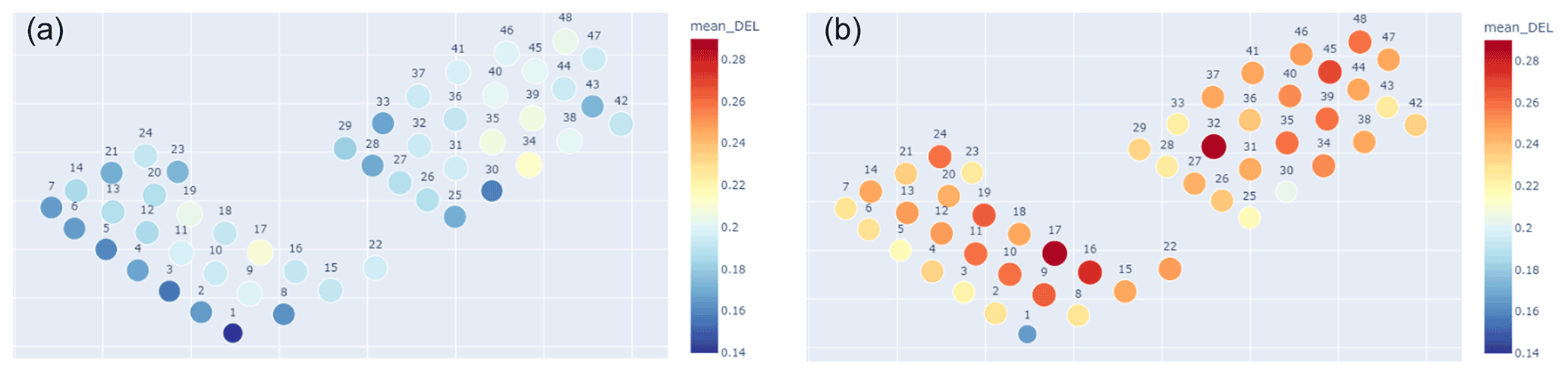
Figure 16 Mean DEL (ratio of the arithmetic mean of all 10 min DELs and the maximum training DEL) farm-wide plot, normalized in relation to the highest training DEL value for (a) scenario F and (b) scenario D.

There are, however, some noticeable exceptions. Several turbines have a lower-than-expected DEL (such as OWT 1 or OWT 30, in blue in Fig. 16). Although there are many underlying phenomena that might contribute to this behaviour, we can start by analysing the power production farm-wide for the same period (Fig. 17, scenario F):

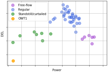
Figure 17 DEL (scenario F) vs. power plotted for the mean values of every turbine of the farm. The lowest DEL turbine – OWT 1 – is shown.

We can see here that there's generally a positive correlation between the turbines which face a lower DEL and the ones that produce less. If we focus on OWT 1 (in orange), which presented the lowest DEL and is on the lower end of the power axis in Fig. 17, we observe that the reason it does not produce so much is due to it being in standstill for a sizeable amount of time during the period investigated. This more frequent standstill, along with OWT 1 usually facing free-flowing wind due to the dominant wind direction, produces the lowest mean DEL of the farm for the period under study. Figure 17 further highlights two distinct sets which present a lower mean DEL: firstly, turbines that were in standstill/curtailed, in green, of which OWT 30 is an example, wherein the lower power output (and thus lower amount of time functioning) is correlated with lower DELs; secondly, turbines that were located in the first string (row of turbines) facing the dominant wind and thus faced mostly free-flow conditions, which enabled both a higher production (higher mean power) and lower DELs, as wake-induced load variations were not present.

Apart from the turbines facing a lower DEL, there are three notable exceptions with a higher-than-expected DEL OWT 34 for Fig. 16a, OWT 32 for Fig. 16b and OWT 17 for both. In Fig. 18 the DEL for each turbine is plotted against the mean fore–aft accelerations (a, scenario D) and against the standard deviation of the fore–aft accelerations (b, scenario F). We can see, for both figures, that OWT 17 is shown to possess an outlier behaviour, presenting both a higher-than-average mean fore–aft acceleration value and standard deviation, where DEL and both of these parameters are positively correlated. The higher variability in the measured accelerations is related to higher DELs (larger cycles). It has been checked whether OWT 17 faces a higher-than-average number of starts/stops, which naturally induce greater loads and DEL.

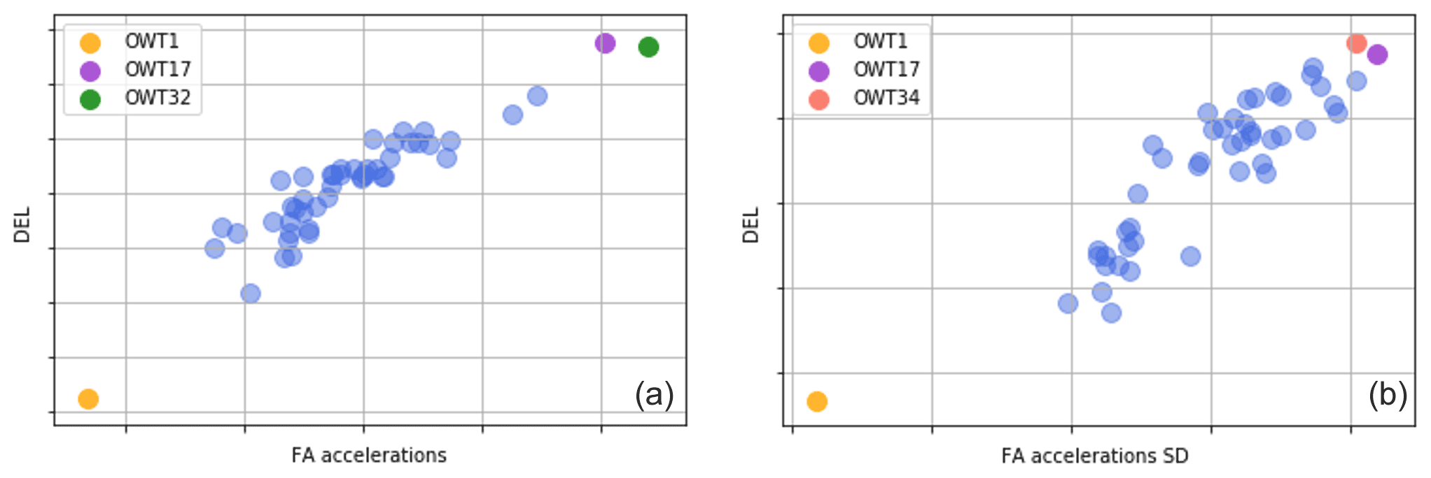
Figure 18 (a) DEL (for scenario D) vs. mean fore–aft low-quality absolute accelerations for every turbine of the farm. OWT 1 is parked, and OWT 17 and OWT 32 are outliers. (b) DEL (for scenario F) vs. the standard deviation of fore–aft accelerations for every turbine of the farm. OWT 1 is parked, and OWT 17 and OWT 34 are outliers.

The main difference between Fig. 16a and b concerns OWT 32 and OWT 34, where the model from scenario D highlights the former and the model from scenario F the latter.

Regarding OWT 32, as Fig. 16b plots the farm-wide DEL for scenario D – a model which includes 1 s SCADA and nacelle accelerations but no thrust load, it can reasonably be assumed that, when including no thrust load, the model will give an added importance to accelerations (referring back to Fig. 1). We can see in Fig. 18a that the mean FA acceleration of OWT 32 far surpasses the average value, where the average fore–aft acceleration value positively correlates with the DEL. If we look back at Fig. 3, this means that the mean value of the FA low-quality absolute accelerations (in green) will have a higher value (offset). This translates, for the top-level SHM FA accelerations, into a greater amplitude (and thus a higher root mean square), which implies that the sensor is seeing more vibrations.

Regarding OWT 34, no apparent unique answer for the higher DEL could be unveiled in the SCADA- or acceleration-based features. However, as seen in Fig. 18b, the standard deviation of accelerations appears to highlight a bit more clearly OWT 34. The answer might indeed lie there – the underlying causal phenomenon might not be picked up solely by SCADA but also by including accelerations and how the model weights their relative importance. It is interesting to note that this turbine in particular presented an unbalanced rotor for this period. The link between acceleration measurements and a higher DEL might lie there. Nonetheless, the 10 min ANN tower FA DEL model is composed by numerous input variables, wherein discerning a single culprit might be difficult, as some behaviours might be the fruit of complex interactions between several parameters, such as thrust load and accelerations.

4 Conclusions

In the current contribution, a methodology to determine jacket-foundation OWT tower bending moment DEL based on artificial neural networks has been successfully implemented. This value can serve wind farm operators in taking informed lifetime-related decisions. The model was validated on two distinct years of data for the training turbine and presented a MAE of around 1 %. Its cross-validation on a different turbine, albeit performing slightly worse (MAE close to 3 %), has proven the applicability of this model to other turbines.

The model uses a reduced set of input data determined by the employment of the recursive feature elimination (using a decision tree classifier estimator) feature selection algorithm. These data are provided by 1 s SCADA (along with the estimation of the thrust load) and SHM accelerometer sensors. A comparative study of feature selection techniques and another of different sensor setups, based on the use of neural networks, have allowed us to identify the sensors and engineered features of greatest importance, as well as which sorts of errors might be related to each instrumentation setup. From this study, it appears that the installation of dedicated tower SHM accelerometers is advisable, as, if a fleet-leader model is to be applied, acceleration data are essential to a good farm-wide generalization. On the other hand, the inclusion of a thrust load model improves overall validation scores, but this does not translate into better cross-validation scores. Further research, in farms with more instrumented turbines, is needed to come to a decision on the added value of quasi-static thrust load.

Finally, this methodology is employed on a farm-wide setting, allowing us to identify turbines with outlier DEL values. By looking at the SCADA and acceleration input data, tentative answers for outlier behaviour can be drawn, providing farm operators with important insights related to maintenance.

5 Future work

Throughout this contribution, the development of this methodology has seen some questions arise, which deserve a deeper look. These questions can be see as future steps in research. Some future research directions include the following:

• application of the current methodology to monopiles;

• employment of other machine-learning algorithms (e.g. SVM, decision trees, kriging, Gaussian process regression, variational auto-encoders) and comparative performance study;

• understanding of the impact of sensor quality (10 min, 1 s, etc.) in a monopile-foundation OWT;

• development of a population-based strategy with training not dependent on only one turbine but on data from possibly several turbines – in particular this seems relevant for the thrust load model that, while improving validation, has resulted in lower cross-validation results;

• utilization of the DEL ANN model to research specific phenomena, such as wind–wave misalignment and wake effect on monopile-foundation OWTs;

• evaluation of which SHM accelerometer placement (bottom level, mid-level or upper level) is the most valuable.

Appendix A

Table A1 Statistical metrics formulae applied to parameter x in which N is the number of individual samples x_i in a 10 min interval.

Appendix B

Table B1 Variable abbreviation explanation.

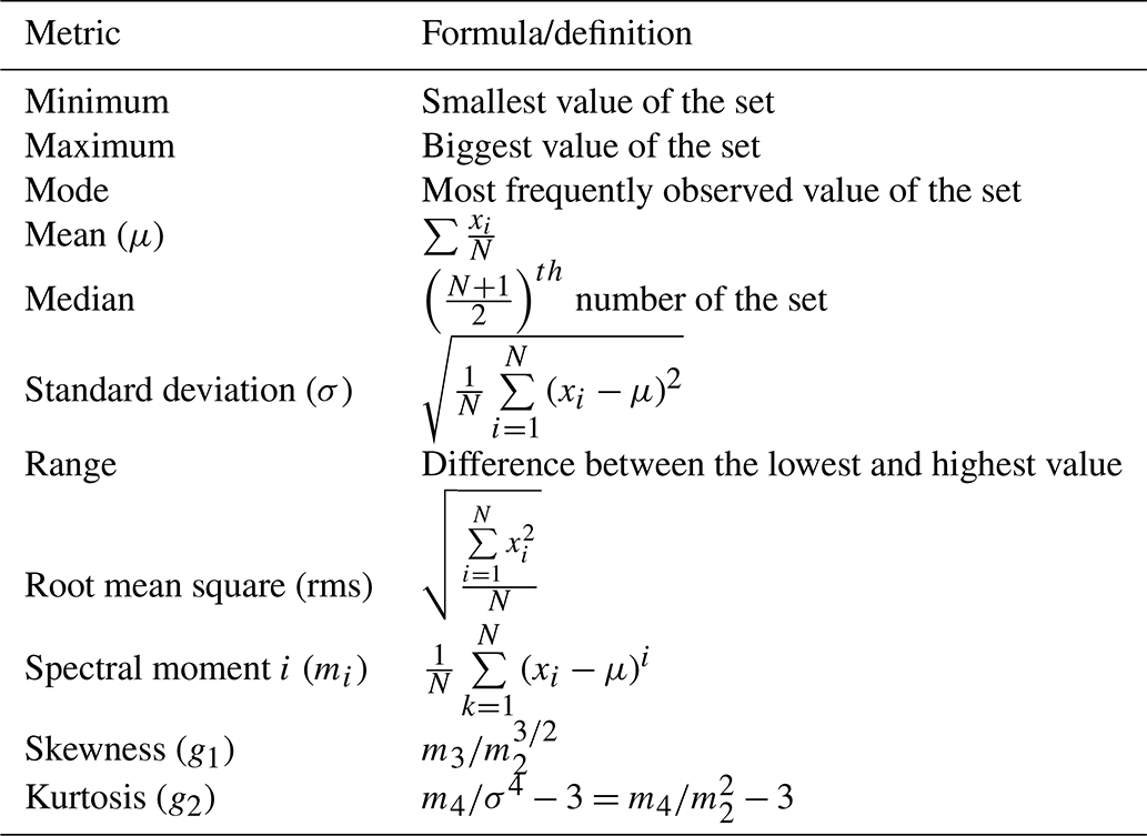
Table B2 Comparative table for different feature selection methods, wherein the differences between the selected parameters/metrics are illustrated. The rows in grey are SCADA-dependent parameters. Note the features ACC FA and ACC SS are the fore–aft and side-to-side accelerations captured by the nacelle's low-quality accelerometer.