the Creative Commons Attribution 4.0 License.
the Creative Commons Attribution 4.0 License.
 | 09 Feb 2022
Optimal closed-loop wake steering – Part 2: Diurnal cycle atmospheric boundary layer conditions
Aditya S. Ghate
Jesús Bas Quesada
Juan José Pena Martínez
Wei Zhong
Felipe Palou Larrañaga
Sanjiva K. Lele
John O. Dabiri
The magnitude of wake interactions between individual wind turbines depends on the atmospheric stability. We investigate strategies for wake loss mitigation through the use of closed-loop wake steering using large eddy simulations of the diurnal cycle, in which variations in the surface heat flux in time modify the atmospheric stability, wind speed and direction, shear, turbulence, and other atmospheric boundary layer (ABL) flow features. The closed-loop wake steering control methodology developed in Part 1 (Howland et al., 2020c, https://doi.org/10.5194/wes-5-1315-2020) is implemented in an example eight turbine wind farm in large eddy simulations of the diurnal cycle. The optimal yaw misalignment set points depend on the wind direction, which varies in time during the diurnal cycle. To improve the application of wake steering control in transient ABL conditions with an evolving mean flow state, we develop a regression-based wind direction forecast method. We compare the closed-loop wake steering control methodology to baseline yaw-aligned control and open-loop lookup table control for various selections of the yaw misalignment set-point update frequency, which dictates the balance between wind direction tracking and yaw activity. In our diurnal cycle simulations of a representative wind farm geometry, closed-loop wake steering with set-point optimization under uncertainty results in higher collective energy production than both baseline yaw-aligned control and open-loop lookup table control. The increase in energy production for the simulated wind farm design for closed- and open-loop wake steering control, compared to baseline yaw-aligned control, is 4.0 %–4.1 % and 3.4 %–3.8 %, respectively, with the range indicating variations in the energy increase results depending on the set-point update frequency. The primary energy increases through wake steering occur during stable ABL conditions in our present diurnal cycle simulations. Open-loop lookup table control decreases energy production in the example wind farm in the convective ABL conditions simulated, compared to baseline yaw-aligned control, while closed-loop control increases energy production in the convective conditions simulated.
- Article
(7520 KB) - Full-text XML
- Companion paper
- BibTeX
- EndNote


Collective wind farm power maximization through wake steering control has demonstrated potential in large eddy simulations (LESs) of idealized atmospheric boundary layer (ABL) conditions (Gebraad et al., 2016), wind tunnel experiments (Campagnolo et al., 2020), and in initial field experiments (Fleming et al., 2019; Howland et al., 2019; Doekemeijer et al., 2021). The primary approach of wake steering control has been open-loop, in which a lookup table of model-optimal yaw misalignment set points is constructed as a function of the incident wind direction, wind speed, and turbulence intensity (Fleming et al., 2019). The set points are optimized using a steady-state, physics-based wake model and applied at the wind farm in time based on an estimate of the incident wind conditions at the farm. However, several challenges arise in open-loop wake steering control, including time-varying ABL flow conditions with measurement uncertainty (Quick et al., 2017; Annoni et al., 2019) and wake model parameter uncertainty (Schreiber et al., 2020; Howland, 2021b), which may lead to a discrepancy between the optimal yaw misalignment set points in the steady-state wake model and the true optimal yaw misalignment values which vary in time.
Recent studies have developed closed-loop control methodologies (Ciri et al., 2017; Campagnolo et al., 2020; Doekemeijer et al., 2020; Howland et al., 2020c) which improve wake steering performance in flow with evolving mean states by incorporating wind farm measurements to modify wind condition (Doekemeijer et al., 2020) and wake model parameter (Howland et al., 2020c) estimates. The reader is directed to Part 1 of this study (Howland et al., 2020c) for further motivation of closed-loop wake steering control. Doekemeijer et al. (2020) investigated the performance of a proposed closed-loop control methodology in LESs of the idealized neutral ABL with a prescribed time-varying wind direction. Howland et al. (2020c) evaluated the performance of closed-loop wake steering control in the conventionally neutral ABL, which is characterized by neutral stratification in the boundary layer capped by a stable free atmosphere (e.g., Allaerts and Meyers, 2015) with fixed boundary conditions. The occurrence of the conventionally neutral ABL is rare in practice since the flow in the boundary layer is generally affected by non-neutral atmospheric stability. While numerical investigations often isolate atmospheric stability to characterize its effects (Abkar and Porté-Agel, 2015), the transition between states of stability influences the ABL structure (Basu et al., 2008b; Fitch et al., 2013) and affects wind farm performance (Abkar et al., 2016). In this study, we investigate the performance of the closed-loop wake steering control methodology developed in Part 1 (Howland et al., 2020c) in the stratified ABL with time-varying wind direction and atmospheric stability.
Wind conditions evolve over the diurnal cycle through modifications to the surface heat flux (Stull, 2012). The daytime ABL is characterized by surface heating and convection, giving rise to enhanced mixing and turbulent kinetic energy. Convective rolls with elongated streamwise length scales are observed for the weakly convective ABL (Deardorff, 1972; Atkinson and Wu Zhang, 1996; Salesky et al., 2017). Conversely, the stratification in the nocturnal ABL suppresses vertical velocity fluctuations and limits the flow length scales (Sullivan et al., 2003). The stable ABL is characterized by enhanced wind speed and direction shear (Wyngaard, 2010) and subgeostrophic (or low-level) jets (Thorpe and Guymer, 1977). Stable ABL low-level jets are generated, in part, by Coriolis-induced wind veer (van der Laan et al., 2021) and by inertial oscillations induced by Coriolis forces (Van de Wiel et al., 2010). Through modifications of the structure of the ABL, stratification influences wind farm performance (Wharton and Lundquist, 2012b).
In some instances, wind farm efficiency is diminished in stable conditions, compared to convective (Barthelmie and Jensen, 2010). Other studies have identified increases in power during stable ABL operation (Wharton and Lundquist, 2012a). Differences in reported wind farm performance in stable ABL conditions may relate to site- and time-specific wind direction shear (Sanchez Gomez and Lundquist, 2020; Howland et al., 2020d) or low-level jets (Gadde and Stevens, 2021). Wind turbines generally operate in time-varying yaw misalignment due to slowly reacting yaw control systems and control error (Fleming et al., 2014). The power production of a wind turbine in yaw misalignment depends on the incident velocity field (Howland et al., 2020d; Liew et al., 2020). Since the wind speed and direction variations over the rotor area depend on the atmospheric stability, the power–yaw relationship for a given wind turbine depends on the stability (Howland et al., 2020d), in addition to the control system in use. While the overall wind turbine performance depends on the interaction between these effects, the influence of stability on wake recovery is more clear. Wakes recover faster in convective ABL conditions compared to stable or neutral conditions (Iungo and Porté-Agel, 2014), and relatedly, the wake meandering is enhanced (Abkar and Porté-Agel, 2015). Provided slower wake recovery as a function of streamwise distance downwind of a wind turbine in stable ABL conditions, wake interactions are generally increased (Abkar et al., 2016). Overall, the potential for wake steering control to increase wind farm power production is anticipated to be higher in stable conditions, and initial empirical results confirm this trend (Fleming et al., 2019).
Wake models parameterize the effects of ABL turbulence on the wake recovery through a prescribed wake spreading rate (Jensen, 1983). Since the wake recovery depends on the atmospheric stability (Abkar and Porté-Agel, 2015), the wake spreading coefficient should depend on the wind conditions. Niayifar and Porté-Agel (2016) proposed a model for the wake spreading rate as a function of the turbulence intensity, but the formulation considers only neutral stability. Instead, we leverage closed-loop control (Howland et al., 2020c) to estimate the wake spreading rate using time-dependent wind farm measurements. Through closed-loop control, the yaw misalignment set-point optimization adapts to the estimated wake model parameters, which vary with atmospheric stability. We anticipate that the primary benefits of the proposed closed-loop control approach result from adapting the model used for set-point optimization to time-varying wind conditions.
The optimal wake steering strategy depends on the wind farm design and the wind conditions, including the wind speed, wind direction, and atmospheric stability. With the effects of turbulent diffusion parameterized with the wake spreading rate, the wind farm flow is estimated using a steady-state wake model with prescribed wind conditions (e.g., Gebraad et al., 2016). Recent studies have extended yaw misalignment set-point optimization to consider wind condition variability and uncertainty about the mean state of yaw misalignment (Quick et al., 2017), wind direction (Rott et al., 2018), and joint yaw misalignment and wind direction (Simley et al., 2020). Howland (2021b) extended methods for set-point optimization under uncertainty to consider wake model parameter uncertainty, and empirical improvements for open-loop and closed-loop control were demonstrated. Quick et al. (2020) estimated the expected value of wind farm power under wind condition uncertainty using polynomial chaos expansion and demonstrated that wind direction uncertainty was the primary uncertainty in determining model-optimal yaw set points.
Beyond wind condition variations about a known mean state, the low-frequency mean state of the atmosphere evolves in time due to mesoscale meteorological processes (e.g., Sanz Rodrigo et al., 2017a) and the diurnal cycle (Kumar et al., 2006; Fitch et al., 2013) and is challenging to forecast. Existing wind farm control reacts to low-pass-filtered wind condition measurements (e.g., Fleming et al., 2019). Since the optimal wind farm control strategy inherently depends on the transient atmospheric conditions, wake steering control based on a forecast of future wind conditions over a finite time horizon is anticipated to improve performance rather than reacting to past data. Recently, Simley et al. (2021) demonstrated in idealized wake model numerical experiments that perfect wind direction preview information slightly improves wake steering control. In this study, we develop a regression-based statistical methodology to forecast future wind direction over a prediction horizon of minutes. We focus on a horizon of minutes based on the timescales of turbine yaw motors. In our approach, the yaw set points are optimized using the wake model and the wind direction prediction rather than the low-pass-filtered historical wind direction data. The performance of wake steering control in transient ABL conditions also depends on the yaw misalignment update frequency (Kanev, 2020), which represents a balance between yaw duty (frequency of yaw motor motions) and reacting to flow features of certain lengths and timescales. In this study, we compare the performance of closed-loop control to open-loop lookup table control for several yaw misalignment update frequency selections.
The set of findings presented here demonstrate the utility of closed-loop wake steering control in more realistic ABL conditions, with time-varying wind direction, wind speed, and atmospheric stability. The potential for wake steering control to increase wind farm power production inherently depends on the atmospheric conditions and the wind farm geometry. To test the closed-loop control methodology, we select a representative, idealized wind farm design and diurnal cycle simulation setup. The effect of wake steering on wind farm energy production will depend on the wind farm and atmospheric conditions of interest. To assess the different control strategies, we focus on controlled numerical experiments in which we modify the wind farm control between cases which have the same wind farm design and incident atmospheric conditions.
This paper represents Part 2 of the closed-loop wake steering control study presented in Part 1 (Howland et al., 2020c). The technical details associated with the model-based wake steering control are detailed in Part 1. Given recent advances in the literature, some methods are updated in this study, and the updates are described in Sect. 2. The diurnal cycle ABL case is described in Sect. 3, and the results are presented in Sect. 4. There are several appendices to provide supporting technical information. The wind direction forecast algorithm is in Appendix A. The diurnal cycle setup is described in Appendix B. The diurnal cycle code validation is presented in Appendix C. Appendix D discusses the initialization of the LES cases for reproducible numerical experiments of wind farm control. Finally, the lookup table construction, for open-loop control, is discussed in Appendix E.
The model-based closed-loop wake steering control methodology used in this study is presented in Sect. 2 of Howland et al. (2020c). Since the publication of Part 1, there have been several additional studies in the literature with improvements to wake steering control methodologies. The updates to the wake steering methodology proposed in Part 1 are introduced in this section.
Several studies have investigated the superposition of individual wind turbine wakes in engineering wake models. Zong and Porté-Agel (2020) propose a momentum-conserving superposition methodology under assumptions of uniform, steady inflow and negligible turbulent transport. Various wake superposition methodologies are investigated for the application of closed-loop control with parameter estimation by Howland and Dabiri (2021), which demonstrated that momentum-conserving and modified linear superposition (Niayifar and Porté-Agel, 2016) perform similarly, while linear superposition (Lissaman, 1979) has degraded predictive accuracy. However, since the momentum-conserving superposition (Zong and Porté-Agel, 2020) requires iterations, it is more computationally expensive than modified linear superposition. Therefore, modified linear superposition (Niayifar and Porté-Agel, 2016) is used in this study (more details are provided in Howland and Dabiri, 2021). The secondary steering model proposed by Howland and Dabiri (2021) is also used.
The power production of a yaw-misaligned turbine depends on the incident flow field (Liew et al., 2020; Howland et al., 2020d). Howland et al. (2020d) developed a blade-element model which predicts the power production of a wind turbine in yaw misalignment given an incident ABL flow and validated the model with utility-scale turbine data operating under various wind speed and direction shear profiles and yaw misalignments. Since the present LES uses non-rotational actuator disk modeling (ADM), the blade element approach is not a representative model. Instead, we use the cosine model, where Pp is a tuned empirical parameter. The Pp exponent depends on the time-varying inflow. Additional inaccuracies arise in the cosine model since the power production as a function of the yaw misalignment is not generally symmetric in non-uniform flow (Howland et al., 2020d; Doekemeijer et al., 2021). Numerical experiments in Part 1 (Howland et al., 2020c) demonstrated that underestimating Pp leads to poor wake steering performance. We select Pp=2.5 for the particular ADM used in this study based on empirical tuning to LESs of the conventionally neutral ABL (Howland and Dabiri, 2021). Since the main purpose of the present study is to characterize the performance of open- and closed-loop methodologies with a shared wake model, we do not dynamically adapt Pp in the closed-loop method in this study. Future work should either use a blade element model to predict the power–yaw relationship for a rotating wind turbine model (Howland et al., 2020d) or adapt Pp depending on the incident flow conditions for a non-rotational model.
Part 1 (Howland et al., 2020c) utilized deterministic programming to optimize the yaw misalignment set points for fixed incident wind speed and direction. In this study, the yaw misalignment set points are optimized using stochastic programming under wind condition (Quick et al., 2017) and model parameter uncertainty (Howland, 2021b). The deterministic and stochastic (optimization under uncertainty, OUU) programming approaches to yaw set-point optimization will be compared. Since the ADM used in this study has fixed CT and Cp as a function of the wind speed, the wind direction is the primary factor influencing the yaw set points (Quick et al., 2020). We therefore consider variations in wind direction α only. The yaw set points are optimized at each control update step with period T. At current time t, the goal of the set-point optimization is to find the optimal yaw misalignment angles for time window t through t+T. The yaw set-point optimization is given by
where is the modeled wind farm power production as a function of the wind direction α, yaw misalignment set-points γs, and wake model parameters ψ. In this study, the wake model parameters to be estimated are the wake spreading rate kw and the Gaussian wake proportionality constant σ0 for each turbine in the wind farm (see Part 1, Howland et al., 2020c). The optimal yaw misalignment set point is . The expected value of the power production is
The probability distributions are indicated by f(⋅). The wake model used in Eqs. (1) and (2) is steady state, which inherently assumes statistically steady-state flow over the time horizon t through t+T. We neglect the wake and rotor dynamics associated with the yaw maneuver (Macrí et al., 2021) and the advection time of the modification to the wake. We account for variations in the wind direction through f(α). The probability distributions are estimated using the wind farm data collected over the window t−T through t, with current time t. The mean wind direction estimate for the next period (t through t+T) is indicated by . The wind direction is assumed to be uniformly distributed between and , where σα is the standard deviation in time of the wind direction measured over the interval T with a sampling rate of Δt, the computational time step in LESs. Previous studies have used Gaussian (Rott et al., 2018; Simley et al., 2020) and Laplacian (Quick et al., 2020) distributions to represent turbulent wind direction variations about a mean state. The diurnal cycle has a non-stationary mean wind direction. With a time-varying flow state, a Gaussian distribution may underpredict the frequency of variations about the mean state. We anticipate that the most appropriate choice of f(α) depends on time-averaging length T, and we recommend that other wind direction probability distributions be considered in future work. Methods for estimating are discussed in Sect. 2.1. The model parameter probability distributions are estimated using the methodology proposed in Howland (2021b), although it is noted that f(ψ) can be estimated using Bayesian uncertainty quantification in future work. Equation (2) is approximated using numerical quadrature with the midpoint rule. The yaw set points are optimized using Eq. (1), solved with gradient-based optimization (Howland et al., 2019). While gradient-based optimization of Eq. (1) may be affected by local extrema, the analytic gradient-based optimization enables real-time set-point optimization on the order of seconds for the eight turbine case considered here. Future work may consider the combination of gradient-free search algorithms and gradient-based optimization. In this study, closed-loop control cases with deterministic yaw set-point optimization are also performed. The deterministic yaw set-point optimization is the method presented in Part 1, with deterministic wind directions and a single set of wake model parameters estimated using the ensemble Kalman filter (EnKF) (Evensen, 2003).
2.1 Statistical wind direction forecast
Existing wake steering control methodologies, including in Part 1, implement yaw misalignment angles based on the low-pass-filtered measurements of the wind direction (see, e.g., Fleming et al., 2019; Howland et al., 2020c). However, due to turbulent and large-scale wind variations, the wind direction varies in time. Methods which react to previous low-pass-filtered wind direction measurements may implement a suboptimal yaw misalignment strategy, depending on the future wind direction trajectory. A recent study using idealized wake model numerical experiments by Simley et al. (2021) demonstrated that using perfect preview wind direction measurements improves wake steering, but using a preview based on a empirically fit cross-spectrum, between the wind direction measurements of two neighboring turbines, did not increase power over the standard method. The empirically fit cross-spectrum model-based wind direction prediction requires measurements of the wind direction by a wind turbine, MET mast, or lidar at an upwind location.
The goal of the optimization (Eq. 1) in closed-loop control is to estimate the optimal yaw set-point angles γs for the time window of t to t+T, during which the yaw angles will be applied. In this study, we use a steady-state wake model for yaw set-point optimization which estimates the time-averaged power production based on time-averaged wind conditions. With perfect wind direction information, the yaw set-point optimization is performed at time t with
We therefore focus on methods to forecast . In this study, two methods are used to estimate , with the estimate given by . The standard approach (termed the filtered method) is which assumes that the moving averaged wind direction is not changing. The moving average is a low-pass filter. We note that some previous approaches used other low-pass filters, such as a first-order low-pass filter (e.g., Simley et al., 2020), rather than a moving average, but we do not anticipate the results of the present study to be substantially different based on the particular wind direction filter used.
Here, we develop an alternative approach to estimate the future mean wind direction based on regression (termed predictive method). The wind direction forecast first uses wind direction data from t−2T to t to identify if the low-frequency wind direction is stationary or varying. A linear regression model is fit to wind direction data from t−2T to t−T. The regression model is then used to predict the wind direction from t−T to t. If the coefficient of determination (R2) of the regression is above a set threshold value of Rmin=0.2 and the regression model has lower mean square error (MSE) than predicting the wind direction from t−T to t as , then the wind direction is considered to be varying; otherwise it is considered stationary. With the low-frequency wind direction determined to be varying, a second regression model is fit to wind direction data from t−T to t. The future wind direction is then predicted using the second regression model at time . If the wind direction is considered stationary, it is estimated as , the default filtered method. The full algorithm is presented in Appendix A in Fig. A1 and Algorithm 1. While this method does not require external upwind wind direction measurements, it could be improved with additional upwind sensors. Closed-loop wake steering cases are performed in LES with both the filtered and predictive wind direction estimates. We selected a linear regression approach for simplicity. We recommend future investigation of methodologies for short-term wind direction forecasting in future work.
Large eddy simulations are performed using the open-source pseudo-spectral code PadéOps (Ghate and Lele, 2017; Ghate et al., 2018). The solver is introduced in detail in Part 1 (Howland et al., 2020c). The LES code has been previously used for simulations of the stable ABL (Ghate, 2018; Howland et al., 2020b). The code is validated for the simulation of the diurnal cycle through a comparison to the LES data of Kumar et al. (2006) in Appendix C. The equation for the transport of the filtered nondimensional potential temperature θ is given by
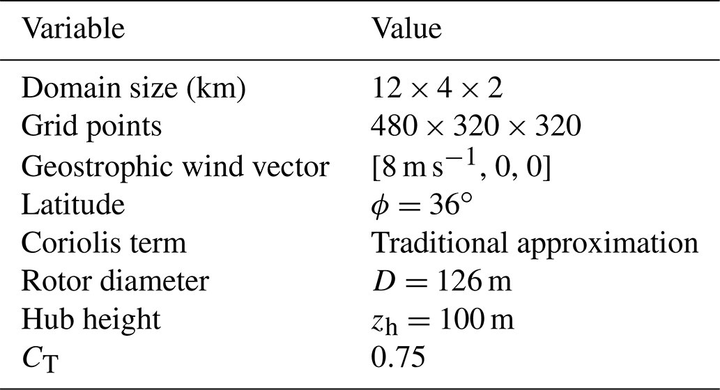
with velocity u, subgrid-scale heat flux with eddy viscosity νT, and turbulent Prandtl number Pr. The wall model is constructed using the SURFFLUX1 algorithm (Basu et al., 2008a) to estimate friction velocity based on a prescribed surface heat flux. The simulation details are provided in Table 1. We use the concurrent precursor methodology to simulate a finite wind farm (see, e.g., Munters et al., 2016; Howland et al., 2020a) with fringe regions (Nordström et al., 1999) in the last 25 % of the domain in the x and y horizontal directions.
A representative diurnal cycle ABL is designed based on the study of (Kumar et al., 2006). The geostrophic wind speed is fixed at G=8 m s−1 and is in the positive x direction. We consider a barotropic ABL with no geostrophic wind shear (baroclinicity). The wind speed is initialized with u=G and throughout the domain. The surface heat flux is prescribed following the time-varying profile shown in Fig. B1a in Appendix B. Further diurnal cycle setup details are provided in Appendix B. The full 24 h diurnal cycle is not simulated since the 12 h period captures the stability transition of interest and for computational limitations. The surface heat flux is initialized at K m s−1, with positive and negative heat flux corresponding to surface heating and cooling, respectively. The convective ABL is run for 1 h to remove startup transience before the wind farm control is initiated. A note on LES initialization for reproducible wind farm control numerical experiments is given in Appendix D.
A nine turbine wind farm is located in the computational domain. The wind turbines are modeled using the ADM. The wind farm geometry is shown in Fig. 1. The turbines are spaced uniformly with distances Sx=6D and Sy=3D in the x and y directions, respectively. Eight wind turbines are considered for wake steering control with one turbine used for reference. Given the initialization in the convective ABL, the wind direction in the ABL will initially be oriented in the positive x direction (Fig. 2a). As the surface heat flux becomes negative, the convective ABL will transition to a stable boundary layer. During the transition, the reduced vertical mixing and inertial oscillations will result in an Ekman spiral, which is characterized by counter-clockwise turning of the wind from the geostrophic wind direction (parallel to isobars) to the surface wind direction (cross-isobaric). As a result, the mean wind direction at the wind turbine hub height will become positive (with the angle measured between the wind direction and the x axis), as shown in Fig. 2a. A zoomed-in wind direction profile between hours 2 and 3 is shown in Fig. 2b to show the turbulent variations. In summary, in the convective ABL, the flow will be approximately in the positive x direction, resulting in wake interactions along the columns of turbines. During the transition and stable regimes, the flow will be oriented with a positive angle, measured from the x axis, and wake interactions will be along the farm diagonals (e.g., turbine 4 in the wake of turbine 1).
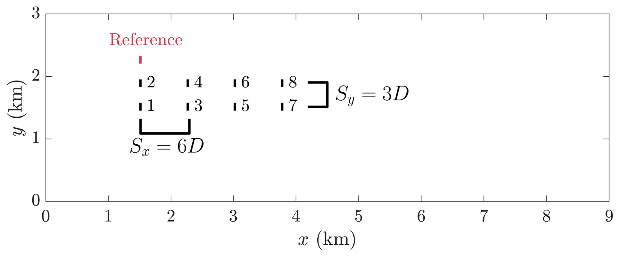
Figure 1The wind farm layout considered in this study within the domain of interest (excluding the sections influenced by the fringe region). The reference turbine (shown in red) is used for power normalization and uses yaw alignment control for each case.
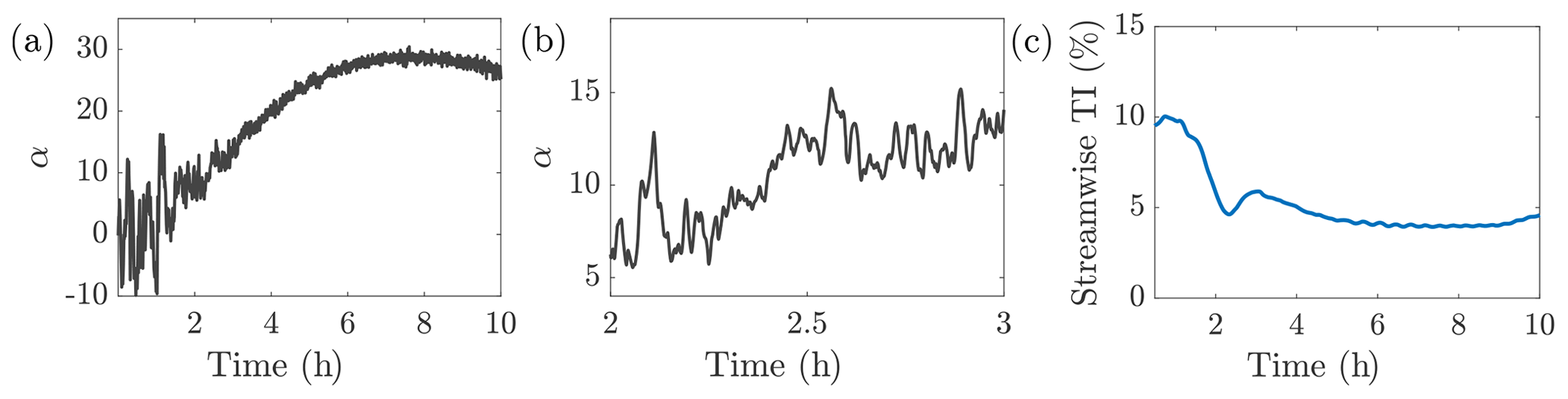
Figure 2Diurnal cycle flow (a) hub-height wind direction, (b) hub-height wind direction zoomed in to show variations between hours 2 and 3, and (c) hub-height turbulence intensity.
The streamwise hub-height turbulence intensity in the inflow to the wind farm, computed from the concurrent precursor, is shown in Fig. 2c. The convective ABL is characterized by approximately 10 % streamwise turbulence intensity. The turbulence intensity decreases below 5 % during stable conditions. The incident wind speed profiles over the diurnal cycle are shown in Fig. 3a. The unstable wind speed has low shear above the near-wall region. As the flow transitions to nocturnal conditions, the shear across the rotor area is enhanced and a subgeostrophic jet emerges. Given the setup of the representative ABL used in this study, the maximum wind speed is above the rotor area. The wind direction as a function of height α(z)−α(zh) is shown in Fig. 3b. The wind direction change over the rotor area is minimal during the convective conditions and is enhanced during stable conditions. The peak veer across the rotor area is approximately 15∘. The stable boundary layer wind direction variation as a function of height z is consistent with Ekman turning (see, e.g., Wyngaard, 2010).
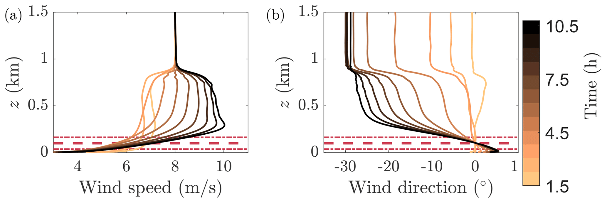
Figure 3Diurnal cycle flow (a) wind speed and (b) wind direction, α(z)−α(zh), as a function of height z, where zh is the wind turbine hub height. The profiles are 30 min averages at hourly intervals throughout the 12 h simulation, with lighter colors near the initialization (unstable ABL) and darker colors corresponding to later times of the simulation (stable ABL). The simulation is initialized at time t=0 corresponding to 18:00. The horizontal dashed line corresponds to hub height, and the horizontal dashed dotted lines are the rotor extents.
As the boundary layer transitions during the diurnal cycle, the structure of the turbulence will be modified, in addition to the mean wind profile changes. An instantaneous hub-height wind speed snapshot during convective conditions is shown in Fig. 4a for wind turbines operating in baseline yaw-aligned control. A zoomed-in image focusing on the wind farm region is shown in Fig. B2. There are large-scale structures of high and low wind speed. The wake meandering is qualitatively seen in the variations in the y position of the wake velocity deficits as a function of x. The mean wind direction at hub height is in the positive x direction during convective conditions. An instantaneous snapshot during stable conditions is shown in Fig. 4b. Compared to the convective conditions (Fig. 4a), the stable flow field has diminished length scales, and the wake meandering is reduced. The wind direction has also shifted, to approximately 20–30∘, with respect to the x axis (see Fig. 2a). A 10 min moving average of the instantaneous flow fields, sampled at a rate of approximately 15 s, is taken for the convective and stable conditions, shown in Fig. 4c and d, respectively. The same time step as the instantaneous snapshots is shown. The 10 min moving average does not eliminate the heterogeneity from the convective ABL flow field. Longer time averages reduce flow field heterogeneity but also average over mean state transitions. Flow field heterogeneity can be physically modeled in future work (e.g., Starke et al., 2021; Martínez-Tossas et al., 2021). Conversely, the 10 min moving average used for the stable conditions removed nearly all inflow heterogeneity. The time-averaged wake regions trailing the individual turbines are qualitatively different in the two atmospheric stability regimes. The effective wake diameters in the time-averaged convective ABL are significantly larger than in stable conditions.
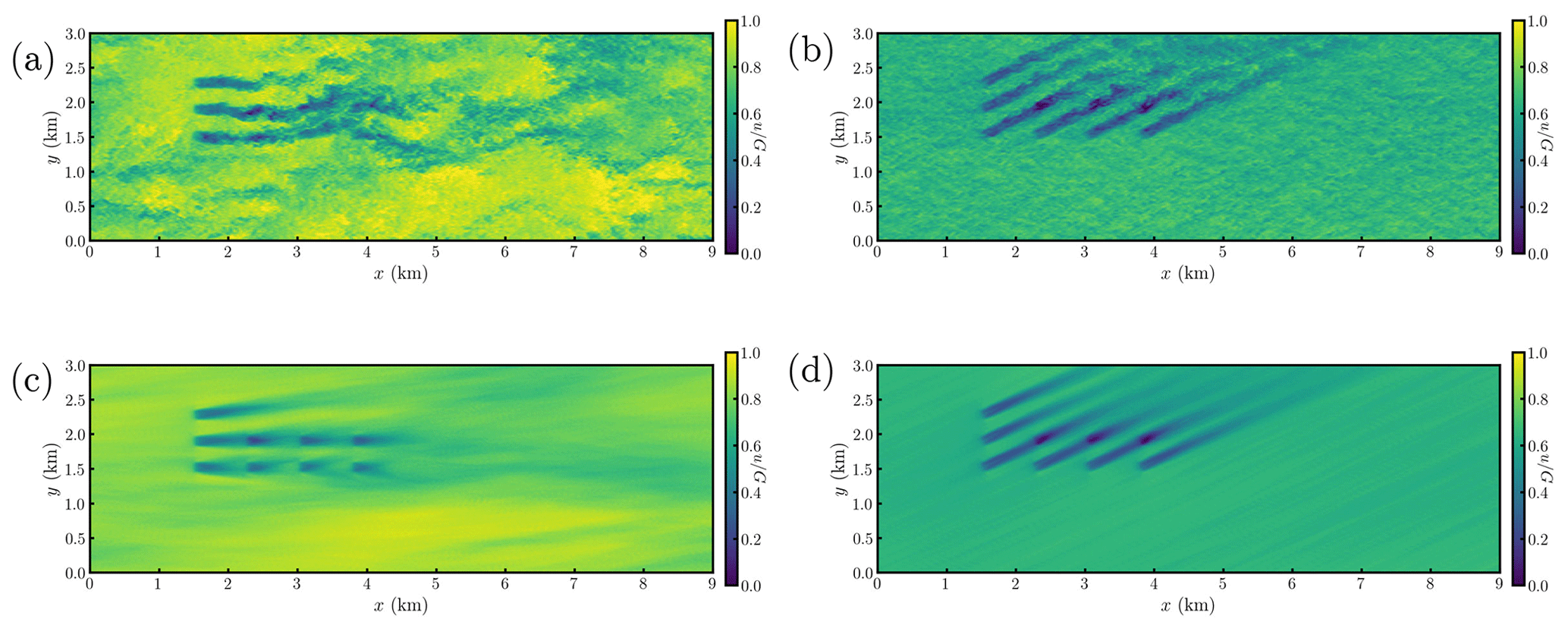
Figure 4Hub-height streamwise velocity during (a, c) unstable and (b, d) stable ABL conditions for the baseline yaw-aligned control case. Instantaneous snapshots are shown in (a) and (b), and 10 min moving averaged flow fields are shown in (c) and (d). The streamwise velocity zoomed in to focus on the wind farm area is shown in Fig. B2.
Table 2The diurnal cycle atmospheric boundary layer wake steering cases. Cases with α forecast checked use the DirectionEstimation (Algorithm 1) to forecast the wind direction over future time T. Cases with optimization under uncertainty (OUU) use the OUU methodology described in Sect. 2. Each case represents a separate LES simulation.
In this section, wake steering control cases are run in the representative diurnal cycle simulation environment discussed in Sect. 3. The wake steering and yaw-aligned control cases are run with a prescribed, fixed yaw update period of T. The wind farm control cases performed in this study are described in Table 2. A baseline, yaw-aligned control case (Case A) is run for reference. As in Part 1, a basic yaw controller is used such that the nacelle position of each turbine is updated to orient towards the mean wind direction measured at each local turbine, averaged over time T. We compare four wake steering control strategies. We consider one open-loop wake steering case and three closed-loop control cases, which differ only through their yaw set-point optimization methods.
Case D (D for deterministic) is closed-loop wake steering with deterministic yaw set-point optimization. The yaw set points are optimized with estimated wake model parameters using the EnKF and mean wind conditions prescribed as the average conditions observed over previous time T. Case D–F (D for deterministic, F for wind direction forecasting) is closed-loop wake steering with deterministic yaw set-point optimization which uses the wind direction forecast methodology. Comparing Cases D and D–F, differences will arise only from the wind direction used in the yaw set-point optimization. Case D uses the mean wind direction measured over the previous time T, while Case D–F uses DirectionEstimation (Algorithm 1) to forecast the wind direction over future time T. Case OUU-F uses optimization under uncertainty (OUU; see Sect. 2) and the wind direction forecast methodology. For brevity, we do not include a case with OUU without the wind direction forecast. Case L uses open-loop lookup table control. The lookup table synthesis is described in Appendix E. In Sect. 4.1, the power–yaw relationship for the freestream turbines is presented. The performance of the various control strategies are compared in Sect. 4.2. The wake model predictions are compared for closed- and open-loop control methodologies. The influence of the yaw update period is considered in Sect. 4.4.
For the purpose of parsing the diurnal cycle results by atmospheric stability, we define the stable regime as (Van Wijk et al., 1990), where L is the Obukhov length:
with friction velocity u*, reference potential temperature θ0, von Karman constant κ, and gravitational acceleration g. For L<0, the flow is unstable or near neutral, while for L>200 the flow is near neutral. Conditions of L<0 and L>200 are combined into unstable and stability transition periods. This stability characterization is qualitative and is used for the interpretation of the results in the following sections.
4.1 Power–yaw relationship
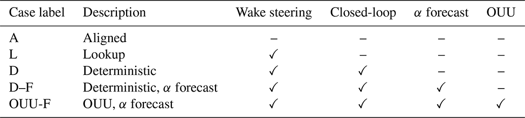
The power productions of the leading two wind turbines in the array, turbines 1 and 2 (see layout in Fig, 1), as a function of their yaw misalignment with respect to the turbine-specific hub-height wind direction, are shown in Fig. 5. The results are shown for a yaw update period of T=30 min, and therefore, each data sample shown is a 30 min average. Since the wind direction changes as a function of time, the magnitude and sign of the model-optimal yaw misalignment set points will also change. Given the incident wind direction and wind farm geometry, turbine 2 will initially misalign the yaw to benefit turbine 4. With the wind direction shifting away from 0∘ with respect to the x axis, there are no turbines downwind of turbine 2 (see Fig. 4b) and its yaw misalignment set point will become zero. Turbine 1 will continue to misalign the yaw to benefit either turbine 3 or turbine 4. The power ratios for the convective ABL are shown with open markers. Given the highly turbulent convective ABL, the finite-time-averaged inflow wind to a given turbine may differ from the winds incident to the reference turbine (see Fig. 4). This effect is not accounted for in the cosine models and is the primary cause for the significant spread in the power ratios in convective conditions.
While there are a limited number of data samples for , the power ratio shown in Fig. 5 appears asymmetric around during stable conditions (filled markers). Given the nocturnal wind speed and direction profiles shown in Fig. 3, the power production for the yawed wind turbines will be asymmetric as a function of the sign of the yaw misalignment angle (Howland et al., 2020d). Considering a non-rotational actuator disk model representation of a wind turbine, the power production is , where u is the incident wind velocity vector and is the unit vector normal to the rotor area. Given the Ekman spiral, negative yaw misalignment, a clockwise rotation of the wind turbine viewed from above, will locally align the turbine above hub height where the wind speed is larger than the hub-height speed (Fig. 3a). Conversely, positive yaw misalignment will locally align the turbine below hub height where the wind speed is lower than hub-height speed.
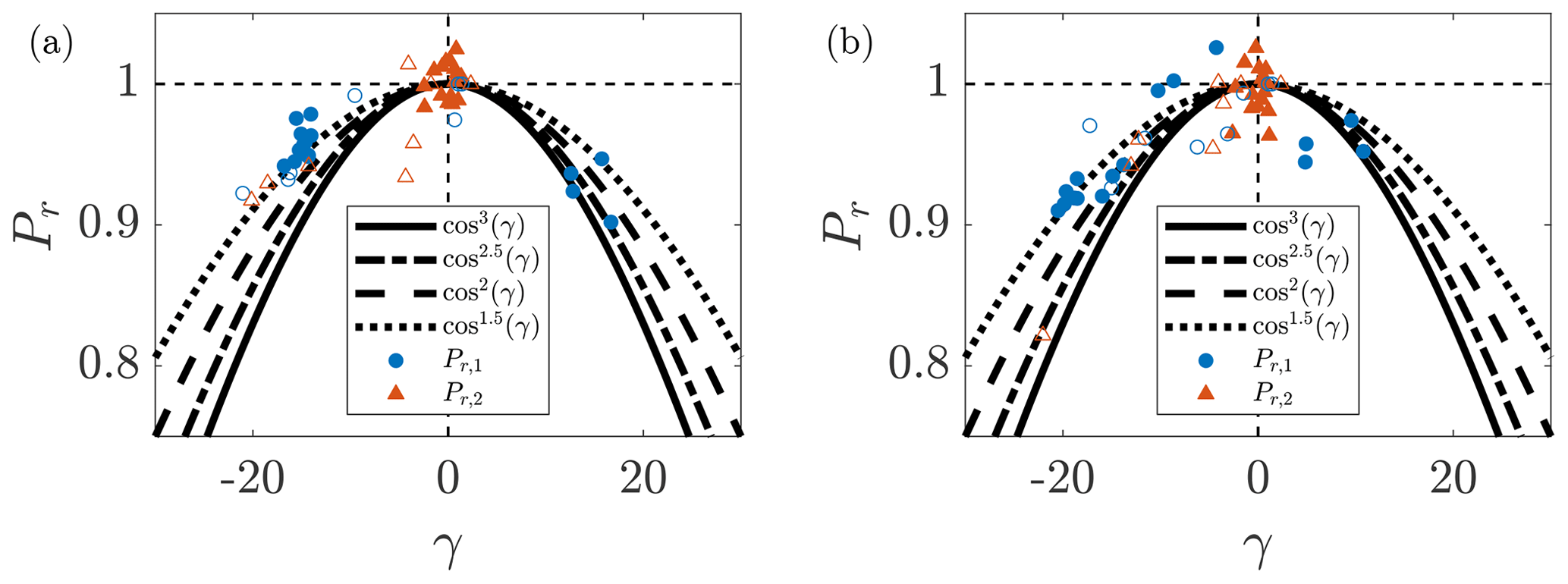
Figure 5Power ratio for turbines 1 and 2 (see layout in Fig. 1) for (a) Case L open-loop lookup table control and (b) Case D closed-loop control shown as a function of the realized yaw misalignment with respect to the hub-height wind direction. Power ratios for stable atmospheric stability (Obukhov length ) are shown with filled markers, and hollow markers are unstable and stability transition periods. The power ratio is averaged for 30 min for each sample.
The power ratio of turbine 1 for negative yaw misalignment is near the cos 1.5(γ) curve. Conversely, the data samples for positive yaw are generally between cos 1.5(γ) and cos 3(γ). In this study, the Pp parameter for the simplified cosine power ratio model was set to Pp=2.5 based on previous tuning in conventionally neutral ABL conditions (see Sect. 2). Since the simplified cosine model is not the focus of the present study, and since the most accurate Pp factor depends on the incident wind profiles and on the sign of γ, the value is not further tuned and is fixed at Pp=2.5 for closed- and open-loop control cases. The results of Part 1 (Howland et al., 2020c) indicate that overestimating the power degradation as a function of the yaw misalignment angle is preferred for wake steering, compared to underestimation.
The power–yaw relationship is often considered for an isolated wind turbine (Howland et al., 2020b), although wake effects have also been considered by (Liew et al., 2020). In this discussion, we have considered the leading turbines in the farm to behave approximately as isolated wind turbines. The leading turbines in the array may be affected by the presence of the downwind turbines, which may alter the power–yaw relationship. This effect may be considered in future work.
4.2 Comparison of control strategies
In this section, the various control strategies introduced in Sect. 4 are implemented in the diurnal cycle ABL flow with a fixed control update period of T=30 min. We first investigate the influence of the wind direction estimation methodologies. The statistical wind direction forecast (Sect. 2.1) is compared to a wind direction estimate using a moving average filter with timescale T. The instantaneous α and mean αT wind direction as a function of time, as measured by the reference wind turbine, is shown in Fig. 6. The mean wind direction estimates using a moving average and using the wind direction forecast methodology are shown, termed filtered αT and predictive αT, respectively. The mean wind direction prediction methods have access to α(0:t), where t is the current time, and predict . In the limiting cases of high wind direction variability around a mean value (hours 0–3) or low mean wind direction changes in time (hours 6–10), the predictive methodology defaults to the same estimate as the filtered value. However, for periods of transitioning mean wind directions (hours 3–6), the predictive wind direction forecast more accurately estimates the mean wind direction for the future time horizon of length T. The mean absolute error (MAE) for the filtered and predictive methods for estimating αT are 1.9 and 1.3∘, respectively. The mean square error (MSE) for the filtered and predictive methods for estimating αT are 6.0 and 3.7 (degrees squared), respectively.
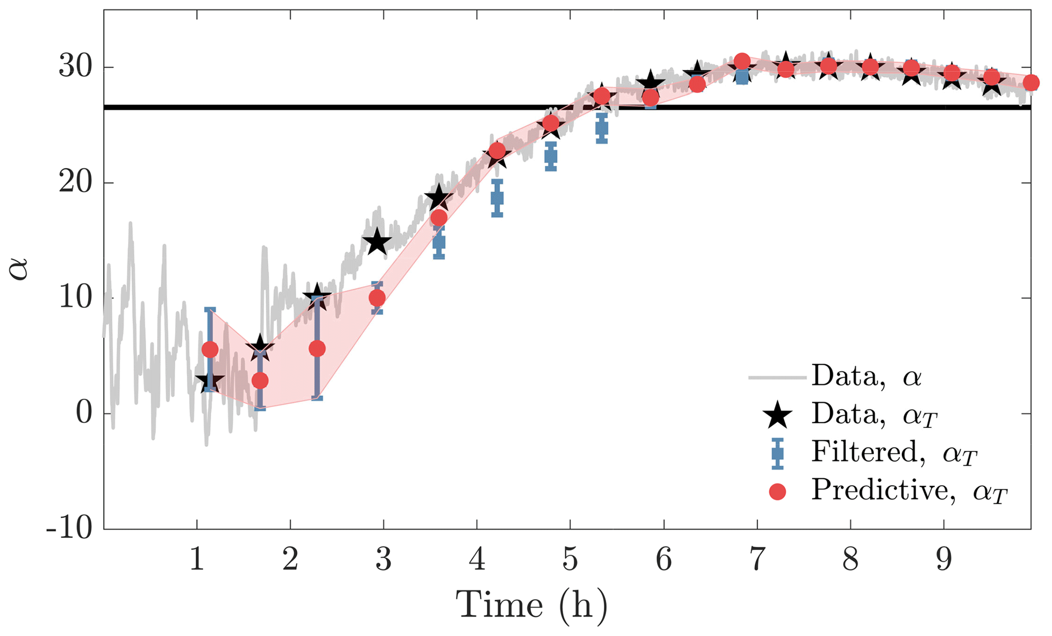
Figure 6Comparison of the mean wind direction estimation methods to the measured instantaneous (α) and mean (αT) wind direction data. A standard approach is shown where the low-pass-filtered wind direction αT is estimated through a moving average. The predictive method is shown in which αT is estimated using the proposed DirectionEstimation algorithm, described in Fig. A1 and Algorithm 1. The horizontal black line corresponds to the wind direction of alignment between turbines 1 and 4.
Closed-loop wake steering control is implemented in the diurnal cycle ABL with deterministic yaw set-point optimization with the filtered (Case D) and predictive forecast (Case D–F) methodologies for the estimation of αT. Two separate LES cases are run with the only difference being the estimated mean wind direction (αT) provided to the yaw set-point optimizer. The yaw set points for turbine 1 are shown in Fig. 7a for the two cases. The realized yaw misalignment angles are shown in Fig. 7b. Since the initial conditions are fixed (the processor topology is also fixed; see Appendix D), during the initial four control update steps in which the filtered and predictive mean wind directions are the same (see Fig. 6), the yaw misalignment values are identical. For step five and beyond, the estimates for the mean wind direction differ, resulting in a divergence of the yaw control approaches. The primary differences between the cases arise between hours 3.5 and 6, during which the mean wind direction transitions over the inflow angle of alignment between turbines 1 and 4. At this inflection point, the optimal yaw set-point angle will transition from positive to negative yaw. The predictive methodology estimates that the wind direction will transition to an angle greater than the inflection point, resulting in a negative yaw set point, while the filtered methodology results in a positive yaw set point. The positive yaw set point, given the resulting trajectory of α, results in wrong-way steering that increases the wake losses at turbine 4.
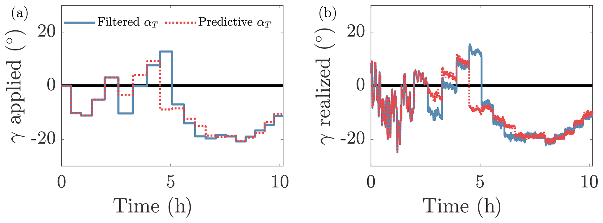
Figure 7Yaw misalignment for turbine 1 (a) applied and (b) realized for the deterministic optimization methodology with filtered (Case D) and predictive forecast (Case D–F) wind-direction-based yaw optimization.
The performance of each case is characterized using an energy ratio,
which quantifies the wind farm performance compared to baseline yaw-aligned control, indicated with γ0, over time interval t1 to t2. The percent gain in energy through wake steering is . We first focus on the time periods in which the filtered and predictive wind direction methodologies differ (control update periods 6 through 9, approximately hours 3.5 to 6). The gain for this time period is −0.1 % and 1.1 % for the filtered (Case D) and predictive (Case D–F) cases, respectively. As a result of the transitioning mean wind direction, reacting to the filtered history of wind direction results in the incorrect yaw misalignment direction, and therefore reduced energy production, compared to baseline yaw-aligned control. Conversely, the predictive wind direction methodology results in the appropriate yaw misalignment set-point direction and increases power compared to baseline control. The energy gain G for Cases D and D–F for the full simulation is shown in Table 3. Overall, the wind direction forecast method increases the energy production using wake steering control in both atmospheric stability regimes, with the predominant energy improvements occurring during the time periods of hours 3.5 to 6, described above.
The energy gain resulting from the use of a wind direction forecast methodology in wake steering control is case specific and depends on several factors. First, the performance gain depends on the fidelity of the predictive methodology. In this study, we have proposed a linear-regression-based wind direction forecast which demonstrates empirical success in this application (Fig. 6). For different ABL forcing, site-specific characteristics, or different update periods T, linear regression may not be sufficient, and other data-driven prediction approaches can be implemented in the framework outlined here (see Appendix A). Future work should consider nonlinear regression or more complex machine learning time series prediction methods. Further, the improvements herein predominantly stem from the occurrence of wind direction changes across the turbine alignment inflow angle. The degree to which a wind direction forecast methodology improves overall wake steering performance will depend on the frequency of such occasions.
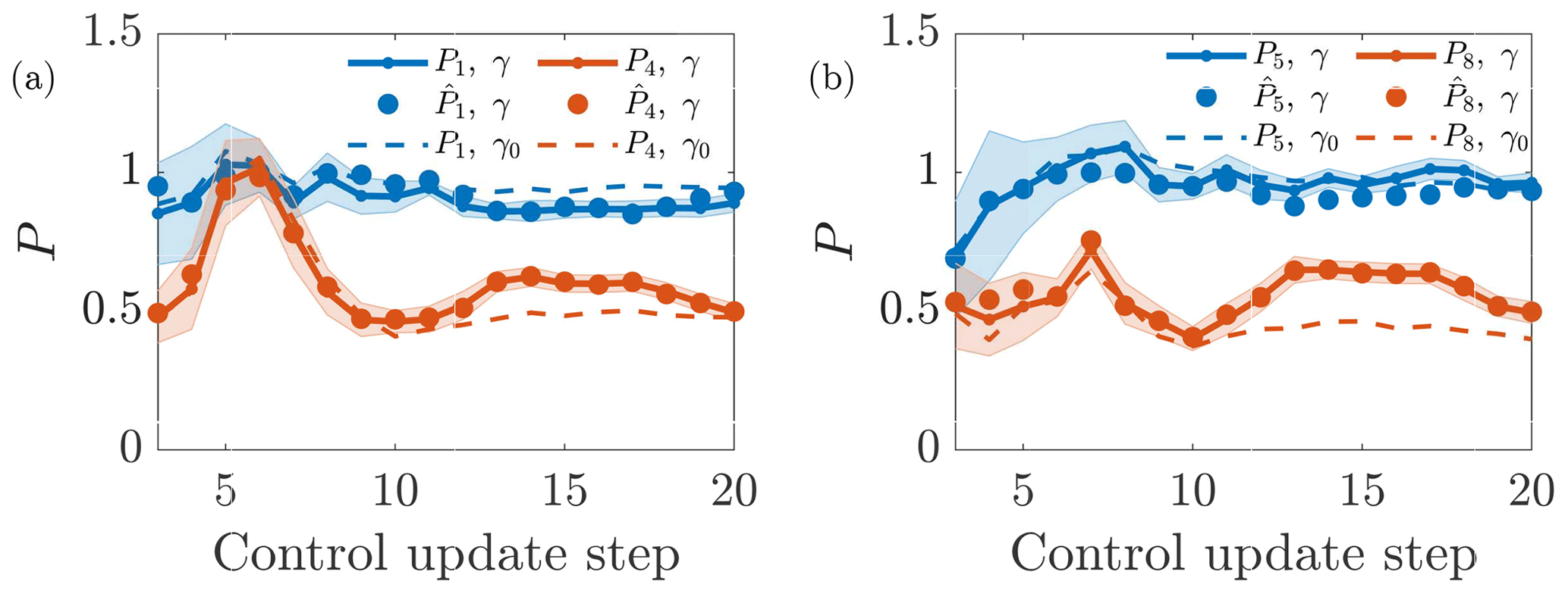
Figure 8Power production results from the closed-loop control Case D and baseline yaw-aligned control cases. The LES power data are given by P, and the wake model estimates are given by . The subscripts on the power denote the turbine number. The yaw-misaligned and yaw-aligned cases are denoted by γ and γ0, respectively.
In the closed-loop wake steering control approach proposed in Part 1 (Howland et al., 2020c), the wake model parameters ψ are estimated at each control update step with time increment T. The LES power production P, γ as a function of the control update step for Case D is shown in Fig. 8. In addition, the wake model power estimates for wake steering control and the LES power production for yaw-aligned control P, γ0 are shown. The power productions for the pair of turbines 1 and 4 are shown in Fig. 8a and for turbines 5 and 8 in Fig. 8b. The wake model estimates for the power production of turbines 4 and 8 exhibit low error, as anticipated because the wake model is calibrated using these data with the EnKF. We test the effect of the EnKF parameter estimation of wake model predictions for out-of-sample data in Sect. 4.3. Larger error arises in the prediction of upwind, freestream power production for turbines 1 and 5, given the simple cosine model (see discussion in Sect. 4.1). The power increase for the downwind turbines is more substantial in the stable regime (control update 9 and after). The estimated wake model parameters are shown in Fig. 9. The parameters are averaged over the upwind turbines 1, 3, and 5. Both the wake spreading rate and the proportionality constant are reduced in stable atmospheric stability, compared to unstable conditions, as anticipated from the time-averaged velocity fields (Fig. 4).
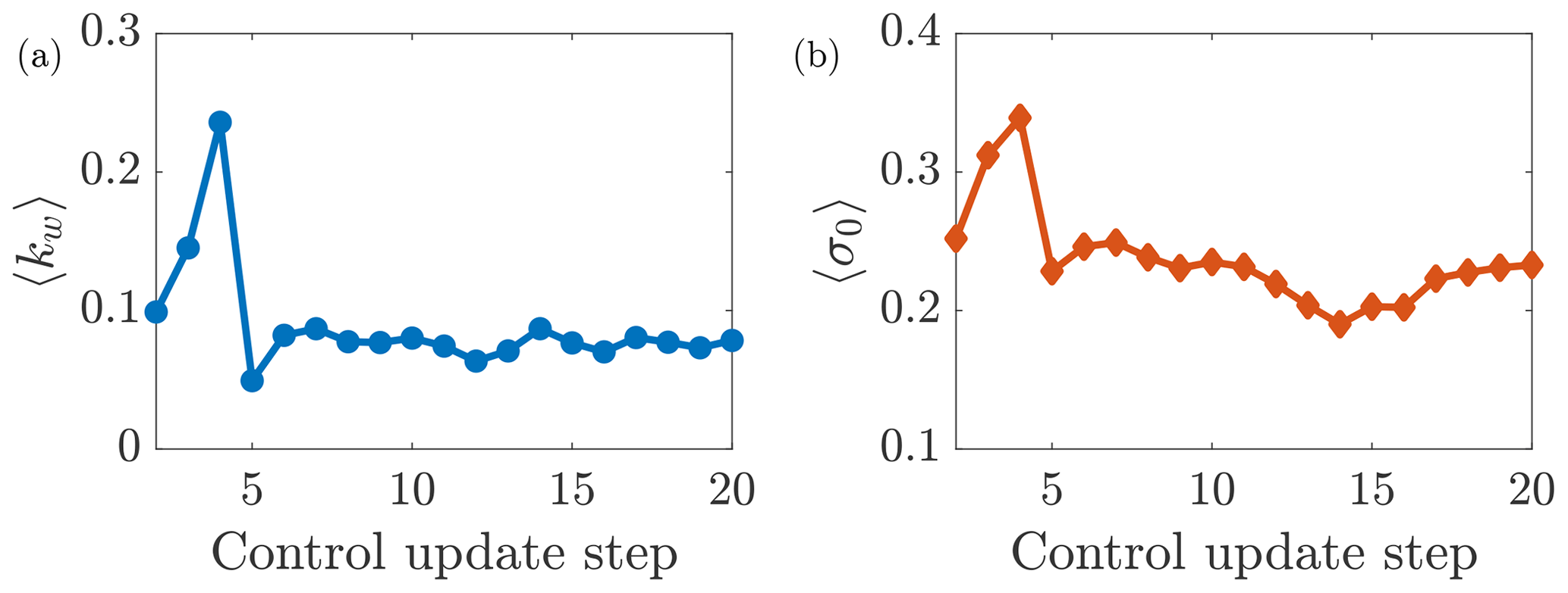
Figure 9Estimated wake model parameters averaged over turbines 1, 3, and 5 as a function of the control update step. (a) Wake spreading coefficient kw. (b) Gaussian wake proportionality constant σ0.
Table 3Wind farm energy production increase compared to baseline yaw-aligned control; with Er in Eq. (6). Cases with α forecast use the DirectionEstimation algorithm. Case OUU-F uses stochastic programming for yaw set-point optimization under uncertainty (OUU). The case with the highest overall wind farm energy production for a given time period is shown in bold. The stable periods correspond to with unstable and transition times otherwise. We note that the hub-height wind direction and wind speed also vary with stability. We denote the approximate mean wind direction at the wind turbine hub height during each stability period with (see Figs. 4 and 6).
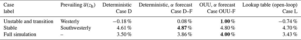
Closed-loop wake steering control is implemented with optimization under uncertainty (see Sect. 2) and the wind direction forecast methodology in Case OUU-F. The energy gain results for Case OUU-F are shown in Table 3. Generally, set-point OUU will reduce the magnitude of the peak yaw misalignment angles, especially near the inflow angle of alignment (see, e.g., Quick et al., 2020). Given the high turbulence in the convective ABL, the wind direction standard deviations are large (see Fig. 6), and the yaw set points will be reduced, compared to deterministic optimization. Case OUU-F has improved performance compared to Case D–F. The OUU (Case OUU-F) has improved performance as a result of increases in energy production during unstable and transition regimes. The energy production is slightly less for OUU in the stable regime. The energy ratio between times t1 and t2 for a given turbine is
with the power production of the reference turbine given by Pref (see Fig. 1 for the layout). The reference turbine is used for normalization rather than to maintain information in the turbine energy ratio metric Er,i about wake losses. The turbine energy ratios for Case OUU-F are shown in Fig. 10. Small reductions in Er,i for yaw-misaligned turbines (1, 3, and 5) result in large increases in energy ratios for the waked turbines (4, 6, and 8). Turbine 7 is not yaw misaligned during the simulation and slightly outperforms the reference turbine likely due to mean flow effects such as induction and blockage in the stable ABL (Segalini and Dahlberg, 2020).
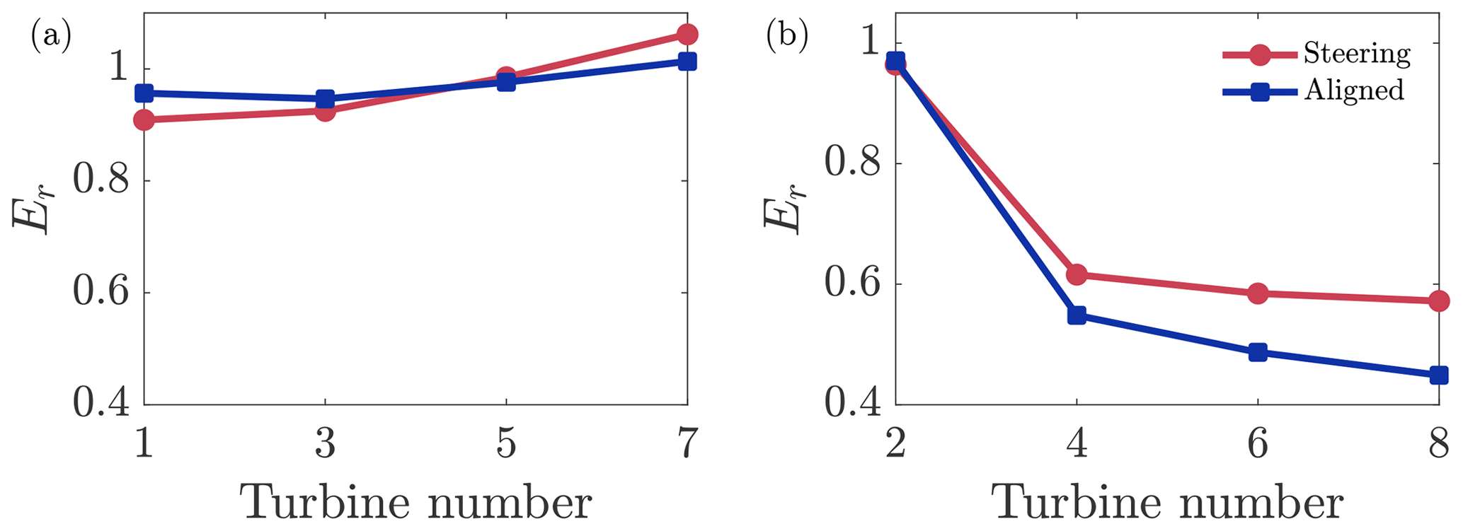
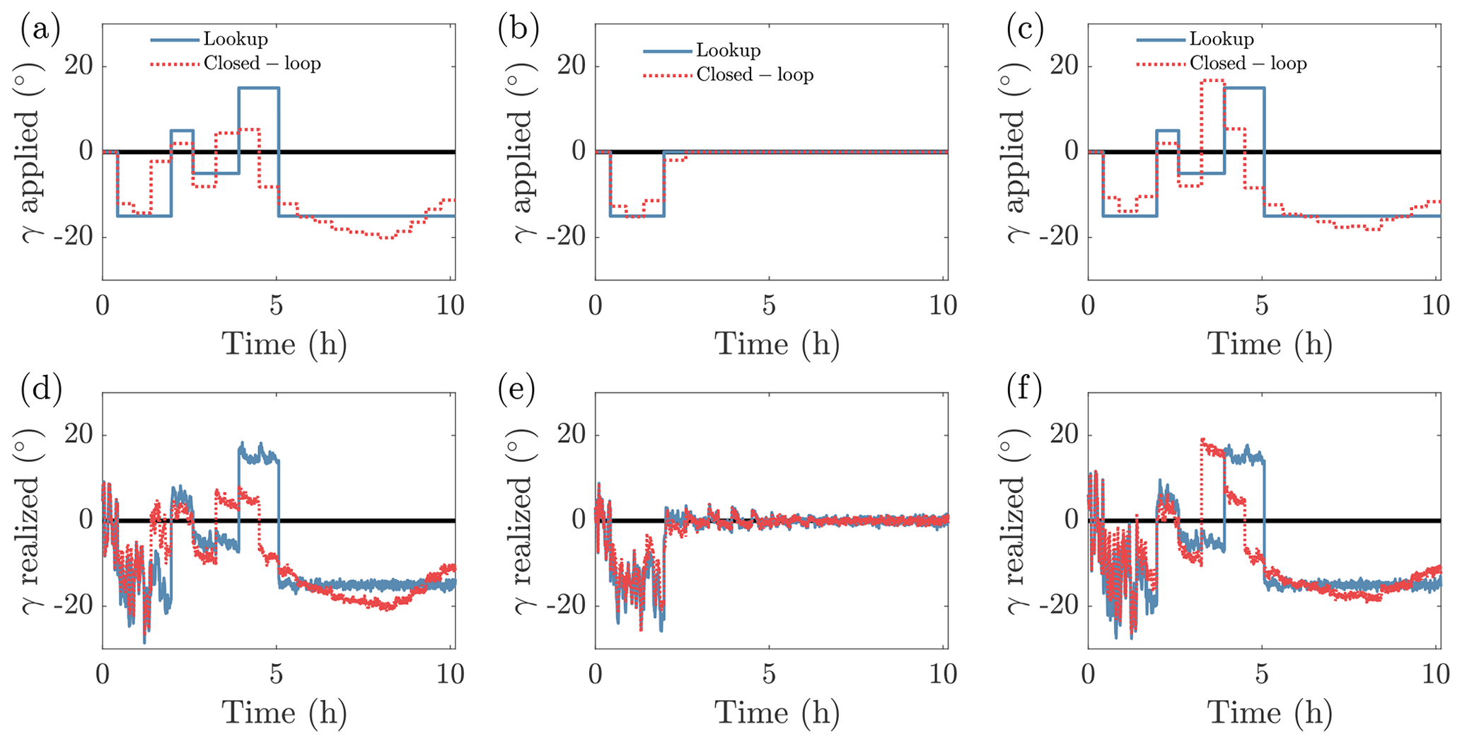
Figure 11Comparison of the yaw misalignment set-point values as a function of time from the OUU closed-loop control (Case OUU-F) and from open-loop lookup table control (Case L) for turbines (a) 1, (b) 2, and (c) 3. (d–f) Same as (a–c) with realized yaw.
Open-loop wake steering is implemented in the diurnal cycle ABL LES (Case L). The open-loop yaw misalignment lookup table synthesis is described in Appendix E. The yaw misalignment set points and realized yaw values for turbines 1, 2, and 3 for closed-loop Case OUU-F and open-loop Case L are shown in Fig. 11. The yaw misalignment set points are qualitatively similar in their approach but quantitatively differ. The differences between the closed- and open-loop yaw set points are larger in the unstable and transition regimes of the simulation than the stable regime. Comparing the yaw misalignment applied in the open- and closed-loop control cases, there are differences in the yaw duty, with the closed-loop control introducing some small amplitude (𝒪(1∘)) higher-frequency variations in the applied yaw. Modifying yaw duty can affect loads on the yaw bearing and other wind turbine components (see, e.g., Hure et al., 2015; Campagnolo and Bottasso, 2021). For open-loop wake steering, the yaw duty depends both on the objective function used to generate the lookup table and on how the lookup table is applied. The objective function used in the optimization step of the closed-loop control considers only farm power production. Future work should incorporate yaw duty penalties in the optimization objective function.
The energy gains for the open-loop wake steering case are shown in Table 3. The lookup table control performance is similar to closed-loop control with deterministic set-point optimization but without the wind direction forecast method (Case D). Lookup table control has less energy production than baseline yaw-aligned control for unstable and transition regimes, with a 0.74 % energy loss. For stable conditions, the open-loop lookup table control has a 4.70 % energy increase over baseline control. Overall, the open-loop control case has diminished performance compared to all closed-loop control cases.
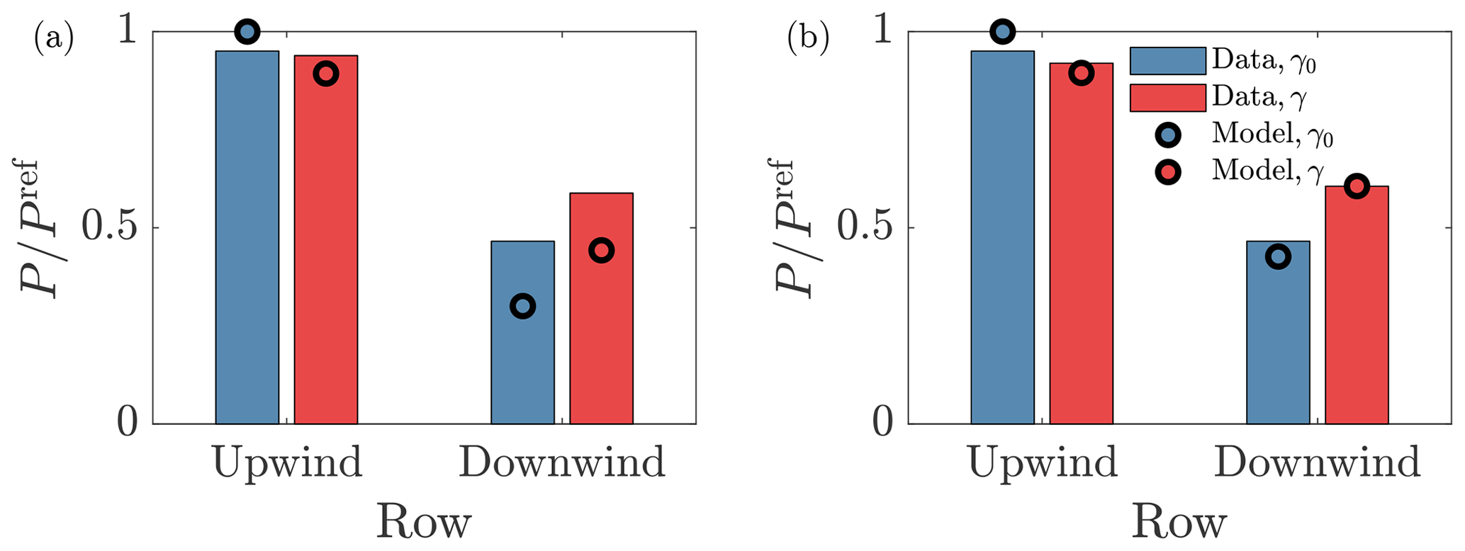
Figure 12Comparison of LES row-averaged power data and wake model predictions for the closed-loop (Case OUU-F) and lookup table (Case L) wind farm control methodologies for the stable stratification regime. (a) Lookup table control data and predictions. (b) Closed-loop control data and predictions. Baseline yaw-aligned control results are indicated with γ0, and wake steering results are indicated with γ. The upwind row is an average of turbines 1, 3, and 5. The downwind row is an average of turbines 4, 6, and 8.
4.3 Wake model predictions
The predictive performances of the open- and closed-loop control methodologies are assessed by comparing the power production predictions from the wake model to the LES power for stable atmospheric conditions. The row-averaged power production is shown for upwind turbines, averaged over turbines 1, 3, and 5, and for downwind turbines, averaged over turbines 4, 6, and 8. The wake model power predictions from open-loop control, using the predefined wake model parameters depending on turbulence intensity in the inflow, are shown in Fig. 12a. The LES power production from the open-loop wake steering case (denoted with γ) is shown, in addition to the baseline yaw-aligned control case (denoted with γ0). The predefined wake model parameters result in significant predictive bias for the downwind waked turbines for both yaw-aligned and wake steering control. The absolute errors are 0.146 and 0.165 for the yaw-misaligned and yaw-aligned wake model estimates, respectively. The LES power production is compared to the closed-loop wake model estimates, in which the wake model parameters are estimated using the ensemble Kalman filter, in Fig. 12b. The ensemble Kalman filter adapts the wake model parameters to accurately estimate the wake steering power production. Since the closed-loop control LES power is used in the Kalman filter, this result is a wake model estimate (training data). Conversely, the wake model estimates for the power production in baseline yaw-aligned control (γ0) are predictions since the Kalman filter does not use the power production from the separate yaw-aligned LES case to estimate wake model parameters. The absolute errors are 0.0004 and 0.039 for the yaw-misaligned and yaw-aligned wake model estimates, respectively.
4.4 Comparison of yaw update periods
In this section, the sensitivity of the wind farm energy production for the various control cases to the yaw set-point update period T is investigated. Baseline yaw-aligned control and three wake steering cases previously described are implemented in LES of the diurnal cycle of the ABL with control update periods of T=30 and T=15 min. Case D is not repeated with T=15 min in this section for brevity. Each case with a specified control update period represents an independent LES simulation. Again, all simulations are initialized from the same initial conditions. The energy gain, with Er in Eq. (6), with respect to baseline yaw-aligned control Case A for T=30 min is shown in Table 4. For yaw-aligned control, decreasing T will increase the frequency of updates, wherein the nacelle position is updated according to the measured wind direction. It is therefore anticipated that reducing T will increase the energy production in yaw-aligned control (see, e.g., Fleming et al., 2014), at the compromise of increased yaw duty (we do not account for the yaw motor energy consumption in this study). Table 4 demonstrates a 0.43 % increase in energy production for the baseline yaw-aligned control with T=15 min, compared to T=30 min.
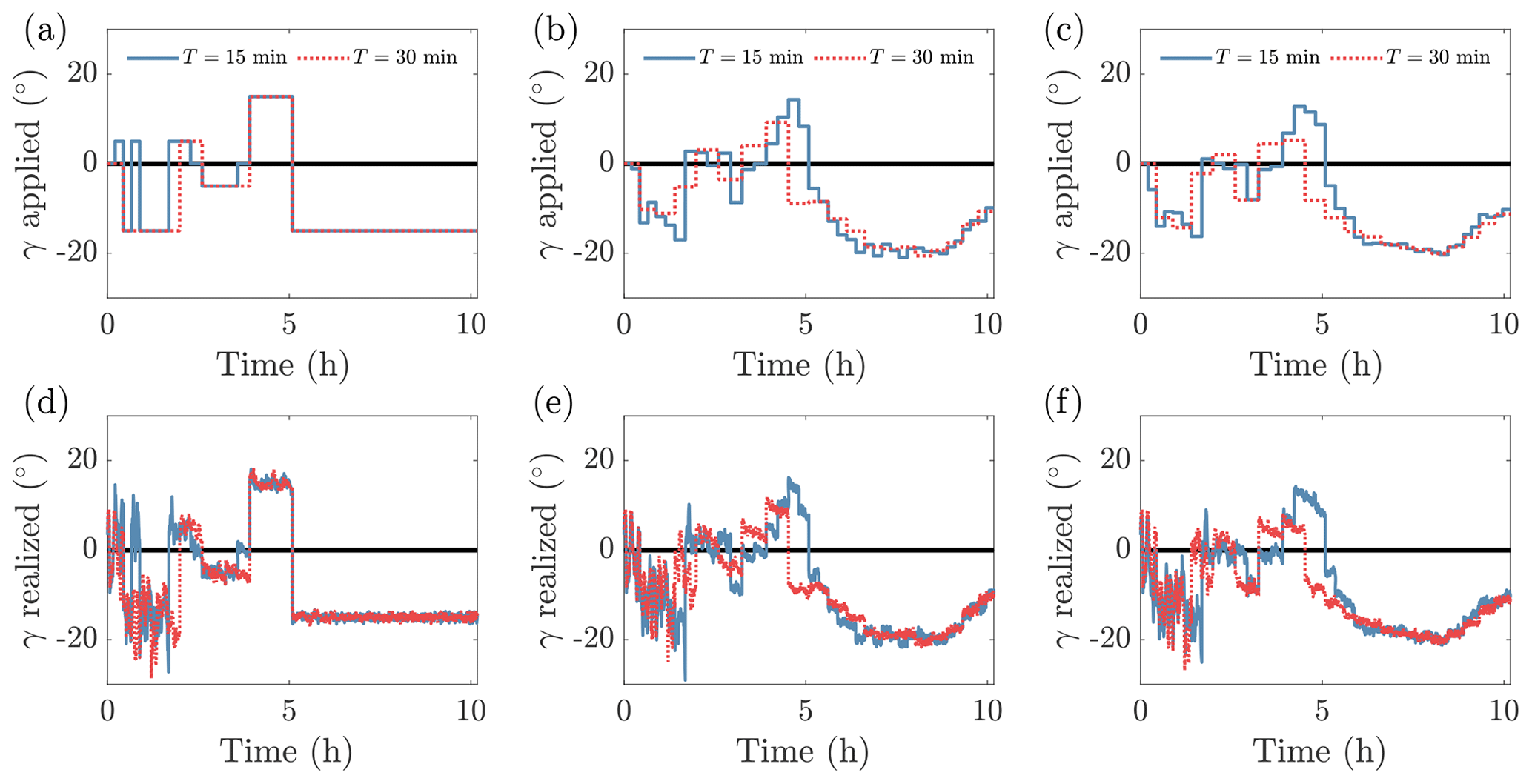
Figure 13Comparison of the yaw misalignment set-point values as a function of time for turbine 1 from the (a) lookup table (Case L), (b) deterministic optimization (Case D–F), and (c) closed-loop control with optimization under uncertainty (Case OUU-F). (d–f) Same as (a–c) with realized yaw.
The wake steering control cases are implemented with T=15 min. The yaw misalignment set points and realized yaw for T=30 and 15 min for open-loop lookup table control (Case L), closed-loop control with deterministic optimization (Case D–F), and closed-loop control with OUU (Case OUU-F) are shown in Fig. 13. A lower control update period increases the variability in the yaw set-point values as the yaw control reacts to higher-frequency timescales. Notably, the T=30 min closed-loop control cases transition to negative yaw misalignment in the stable regime (around 5 h) sooner than the faster update frequency cases (T=15 min). For T=15 min, the wind direction forecast method defaults to the moving average filter for most time steps. For T=30 min, the wind direction forecast results in negative yaw misalignment angles as the flow is transitioning across the inflow angle of turbine alignment (proactive) rather than after the transition has occurred (reactive).
Table 4Wind farm energy production increase compared to baseline yaw-aligned control with T=30 min; with Er in Eq. (6). Cases with α forecast use the DirectionEstimation algorithm. The case with the highest overall wind farm energy production is shown in bold. The full simulation period is considered, with stable, unstable, and transition regimes.

The energy gain for each case with respect to the energy production in baseline yaw-aligned control with T=30 min is shown in Table 4. The highest energy production among all cases considered is optimization under uncertainty (Case OUU-F) with the wind direction forecast methodology and T=15 min. The reduced yaw update period increases the energy production of closed-loop wake steering performed with OUU (Case OUU-F), while it slightly decreases the energy production of closed-loop wake steering with deterministic set-point optimization (Case D–F). There are several factors which contribute to this result. The closed-loop control method estimates wake model parameters based on the average power measurements. For the closed-loop control methodology used here, the moving average for wind turbine power production uses the same timescale T used by the control updates. Therefore, reductions in T also reduce the time averaging length of the power production, which is used for parameter estimation. The reduction in T increases the variability in the mean power data by the central limit theorem. Reductions in T may therefore lead to higher variability in the estimated wake model parameters. However, the averaging and control update timescale T must be sufficiently small to adapt the wind farm control to the time-varying mean wind conditions. The selection of T is a trade-off between these competing effects and may be site and ABL condition specific. While the optimal selection of T is not the focus of this study, T=15 min empirically demonstrates the highest overall energy production in these LES cases. The optimal update period should be investigated jointly with wind condition forecast methodologies. Future work should consider decoupling the parameter estimate and control updates.
Contrary to deterministic set-point optimization, Case OUU-F, which utilizes set-point optimization under model parameter uncertainty, has improved performance with decreasing update periods T. This empirical result is also reproduced for unstable ABL conditions in Howland (2021b). Optimizing yaw misalignment set points under a distribution of model parameters reduces the sensitivity to noise in the wind farm power production data. The effect of reducing the yaw update period for open-loop control is anticipated to be similar to baseline yaw-aligned control since the yaw set points have been pre-defined in the lookup table. The energy production from open-loop control is increased by 0.4 % by reducing T to 15 min. For T=15 min, open-loop lookup table control (case L) has a similar performance to closed-loop control with deterministic optimization (Case D–F). Closed-loop control with yaw set-point OUU (Case OUU-F) has the highest energy production for both yaw update periods, and the highest overall energy production occurs with T=15 min.
The closed-loop wake steering control methodology, developed in Part 1 (Howland et al., 2020c) is extended here. We compared closed-loop wake steering to baseline yaw-aligned control and open-loop lookup table control in idealized large eddy simulations of the diurnal cycle for yaw set-point update periods of T=15 and 30 min. The effect of wake steering on energy production depends on the wind farm geometry and the atmospheric conditions. For the idealized wind farm and ABL setup considered here, wake steering has a larger increase in energy production for stable ABL conditions than for convective. Importantly, other details of the flow, such as hub-height wind direction and speed, change along with stability in the diurnal cycle simulations presented in this study. Therefore, the present diurnal cycle simulations do not represent controlled experiments to isolate the effects of the stability on wake steering control. Such controlled experiments are suggested for future work.
Open-loop lookup table control and closed-loop wake steering control with deterministic set-point optimization have reduced energy production in convective conditions compared to baseline yaw-aligned control in the considered cases. Closed-loop wake steering with set-point optimization under uncertainty increases energy in convective conditions, compared to baseline control. The highest overall energy production is achieved with closed-loop wake steering with yaw misalignment set-point optimization under wind direction and model parameter uncertainty for T=15 min. Reducing the yaw set-point update period increases the energy production for all cases except for closed-loop wake steering control with deterministic set-point optimization, in which the yaw set points are influenced by data measurement noise. The influence of the data measurement noise is alleviated with set-point optimization under uncertainty.
The optimal yaw misalignment set points depend on the incident wind direction. Rather than assuming that the future wind direction will be equal to the low-pass-filtered recorded wind direction data, in this study, we develop a regression-based wind direction forecast. The wind direction forecast uses two previous time windows to identify if the wind direction is stationary or varying in time. If the wind direction is stationary, the standard filtered wind direction is used. If the wind direction is identified to be varying in time, a linear regression is used to forecast the future wind direction. The proposed framework can be used with arbitrary wind direction time series estimation methods. Future work should consider nonlinear regression or more complex time series machine learning methodologies, such as recurrent neural networks.
The results of Part 1 and 2 of this study suggest several directions of future work. Future work should investigate the optimal yaw set-point update period in tandem with wind condition prediction methodologies. Since the closed-loop control method impacts yaw duty, realistic utility-scale turbine yaw duty penalties, based on yaw motor energy usage and increased maintenance costs, should also be considered in the set-point optimization. Improved estimates for the wake model parameter probability distributions with physical constraints should be considered. Additionally, future work should consider model form uncertainty and modeling error in connection with model parameter estimation. Future studies should compare various model-based closed-loop wake steering approaches which use steady-state and dynamic wind farm models to model-free closed-loop wake steering control.
We note that the simulations presented in this study are an idealization of the diurnal ABL with fixed geostrophic wind speed and direction (Beare et al., 2006; Svensson et al., 2011; Fitch et al., 2013). While observations occasionally demonstrate approximately steady geostrophic winds over timescales up to a day (Bosveld et al., 2014), variations in the large-scale forcings in the atmosphere influence the ABL (Muñoz-Esparza et al., 2017) and wind farm flows (Sanz Rodrigo et al., 2017a, b). Methodologies to investigate wake steering control in more realistic ABL wind conditions through meso-microscale coupling should be considered in future work. Finally, future work should consider wake steering in complex terrain.
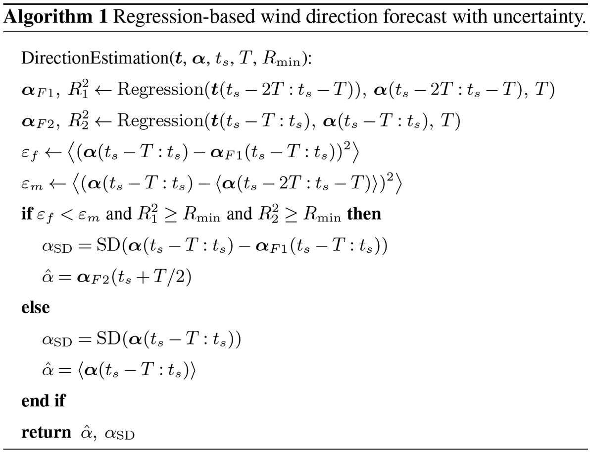
The regression-based statistical wind direction forecast discussed in Sect. 2.1 is described in this section. A schematic of the algorithm is shown in Fig. A1. The algorithm is presented in Algorithm 1. The inputs are the measurement time series t, the measured wind direction time series α, the current time ts, the yaw set-point update period T, and the minimum coefficient of determination value Rmin. The algorithm Regression() is provided time and wind direction vectors and uses linear regression to estimate the wind direction over the next time period of length T (αF). Averaging is denoted by 〈⋅〉, and standard deviation is denoted by SD.
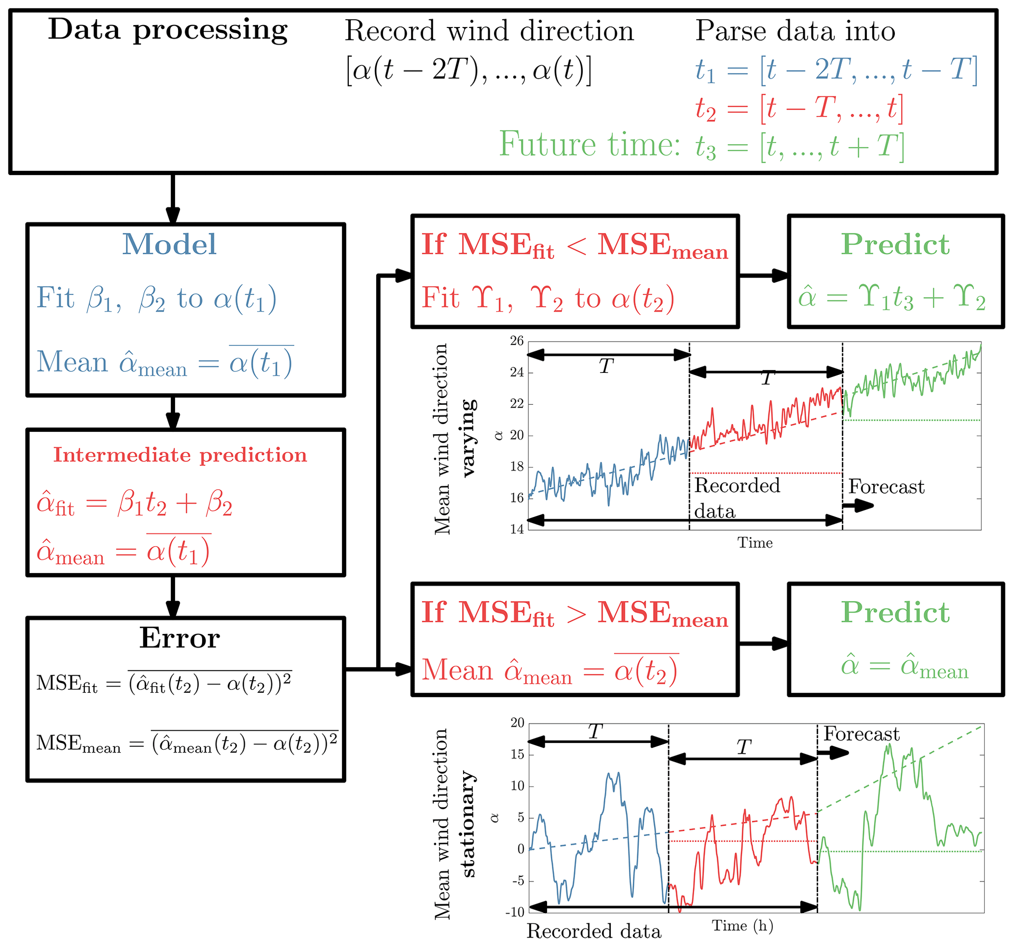
Figure A1Wind direction estimation algorithm DirectionEstimation. Dashed lines are wind direction predictions using regression, and dotted lines are predictions using the mean values.
The surface heat flux boundary condition used in the idealized diurnal cycle simulation is shown in Fig. B1a. The initial potential temperature profile is shown in Fig. B1b. The streamwise velocity at the wind turbine hub height, zoomed in to the wind farm region, is shown in Fig. B2.
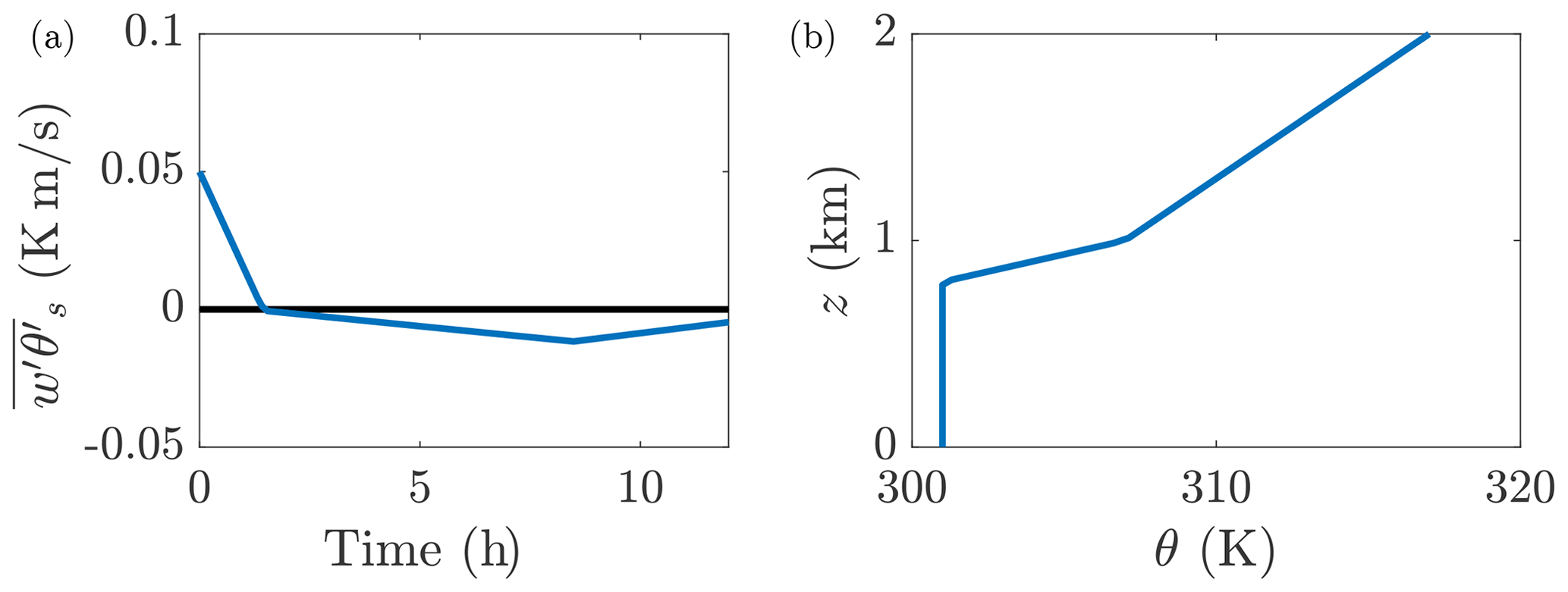
Figure B1(a) Time-varying surface heat flux . The simulation is initialized at time t=0 corresponding to 18:00. Positive heat flux corresponds to surface heating, and negative flux is cooling. (b) Initial potential temperature θ profile.
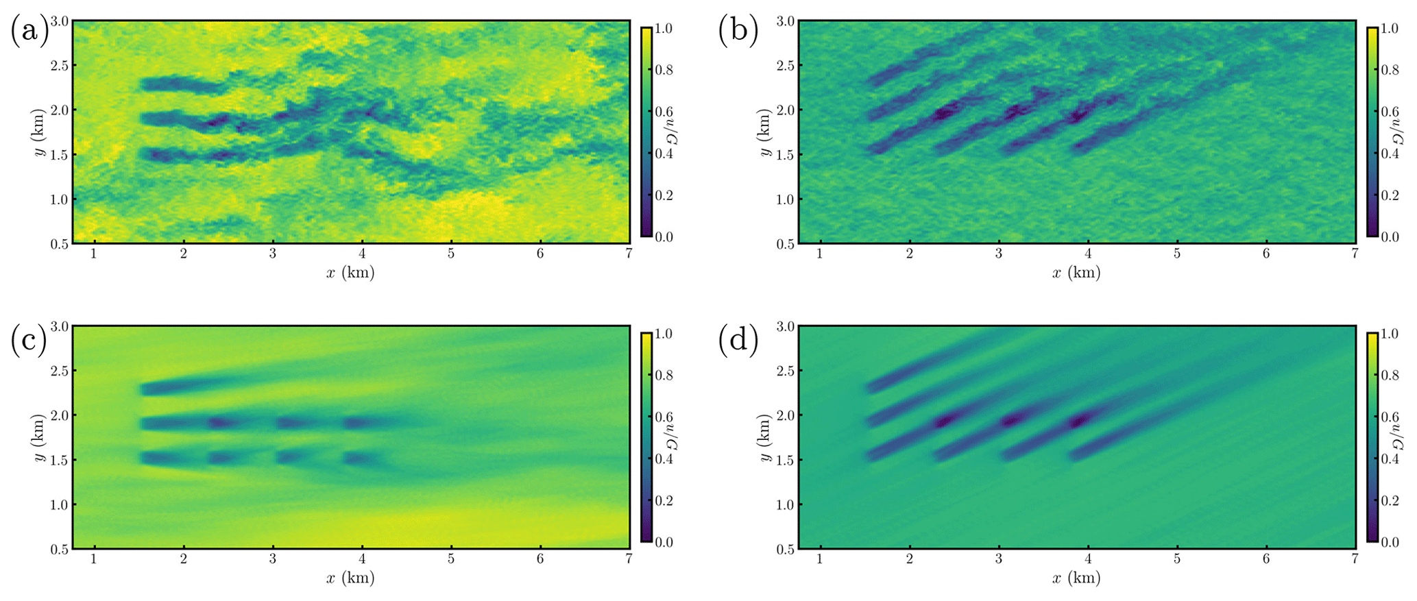
Figure B2Zoomed-in hub-height streamwise velocity during (a, c) unstable and (b, d) stable ABL conditions for the baseline yaw-aligned control case. Instantaneous snapshots are shown in (a) and (b), and 10 min moving averaged flow fields are shown in (c) and (d). The streamwise velocity in the full domain is shown in Fig. 4.
The diurnal cycle implementation in PadéOps (Ghate, 2018) is validated in this section. The diurnal cycle LES case of Kumar et al. (2006) is used as a reference. The boundary conditions constructed in Kumar et al. (2006) correspond to the HATS field campaign (Horst et al., 2004). The full details of the diurnal cycle initialization are provided in (Kumar et al., 2006). The free atmosphere is in geostrophic balance. Only the vertical component of Earth's rotation is included (traditional approximation is enforced; Howland et al., 2020b). The prescribed geostrophic wind speed and surface heat flux are shown in Fig. C1.
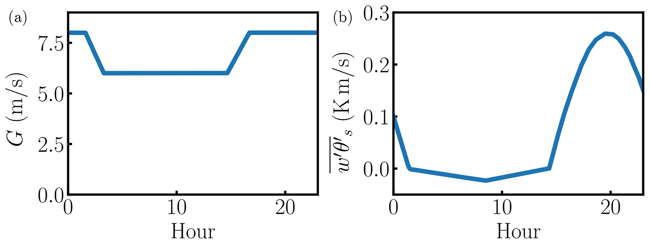
Figure C1Diurnal cycle validation case (Kumar et al., 2006). (a) Diurnal cycle geostrophic wind speed. (b) Diurnal cycle surface heat flux .
The validation focuses on two integrated quantities in the ABL. The friction velocity is shown in Fig. C2a. There is sufficient agreement between the present LES and the reference case. The boundary layer height zi, normalized by the Obukhov length, is shown in Fig. C2b. There is qualitative agreement between the cases with some quantitative discrepancy in the stability transition regions of the profile. The quantitative discrepancies in the normalized boundary layer height are primarily the result of the differing numerics and subgrid-scale models used in the two simulations. Primary discrepancies arise in the stable ABL since the Ozmidov scale is of the same order as the grid spacing (Sullivan et al., 2016). The present LES uses a sixth-order compact finite difference scheme (Lele, 1992) in the vertical direction, whereas Kumar et al. (2006) implemented a second-order finite difference scheme. Overall, the results suggest that the diurnal cycle boundary condition implementation is sufficient for the simulation of a representative diurnal cycle of the ABL.
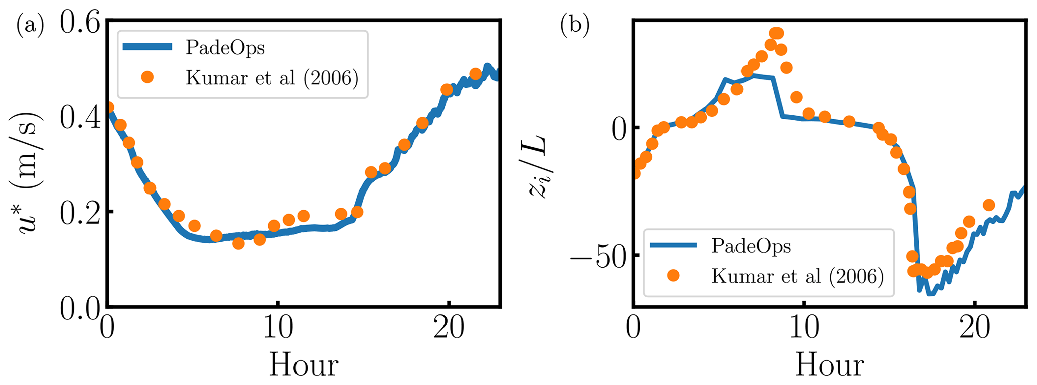
Figure C2Diurnal cycle validation case (Kumar et al., 2006). (a) Diurnal cycle friction velocity u*. (b) Diurnal cycle boundary layer height normalized by the Obukhov length . Details for boundary layer height estimation provided in Kumar et al. (2006).
Since turbulent flows exhibit a chaotic dependence on initial conditions (e.g., Pope, 2001), the initial conditions for all LES cases presented in this study are executed from the same initial conditions. Further, differences in parallel processor topology can result in round-off errors which will exponentially grow to 𝒪(1) differences in the instantaneous flow fields. In this section, we highlight the differences that arise in the comparison of separate wind farm control LES cases due to the chaotic nature of turbulence. Two simulations of open-loop lookup table control are implemented in the diurnal cycle simulations described in Sect. 3. The lookup table methodology is described in Appendix E. The simulations are started from identical initial conditions but with different parallel processor topology, which will result in an initial round-off error difference (10−8) between the cases. The reference turbine wind directions are shown in Fig. D1a, and the applied yaw misalignments are shown in Fig. D1b. While the differences between the cases appear minor visually, they differ in their energy ratio results. The energy gains for the two cases with respect to baseline yaw-aligned control are 3.43 % and 3.17 % for cases 1 and 2, respectively. The primary differences arise in convective ABL conditions, in which the energy gains are −0.74 % and −1.69 % for cases 1 and 2, respectively. Conversely, the differences in stable conditions are minor, with gains of 4.70 % and 4.72 % for cases 1 and 2, respectively. Overall, the results suggest that the initialization and parallel processor topology round-off must be identical to machine precision to ensure accurate comparisons between LES control cases. Primary differences arise in ABL conditions with high turbulence.
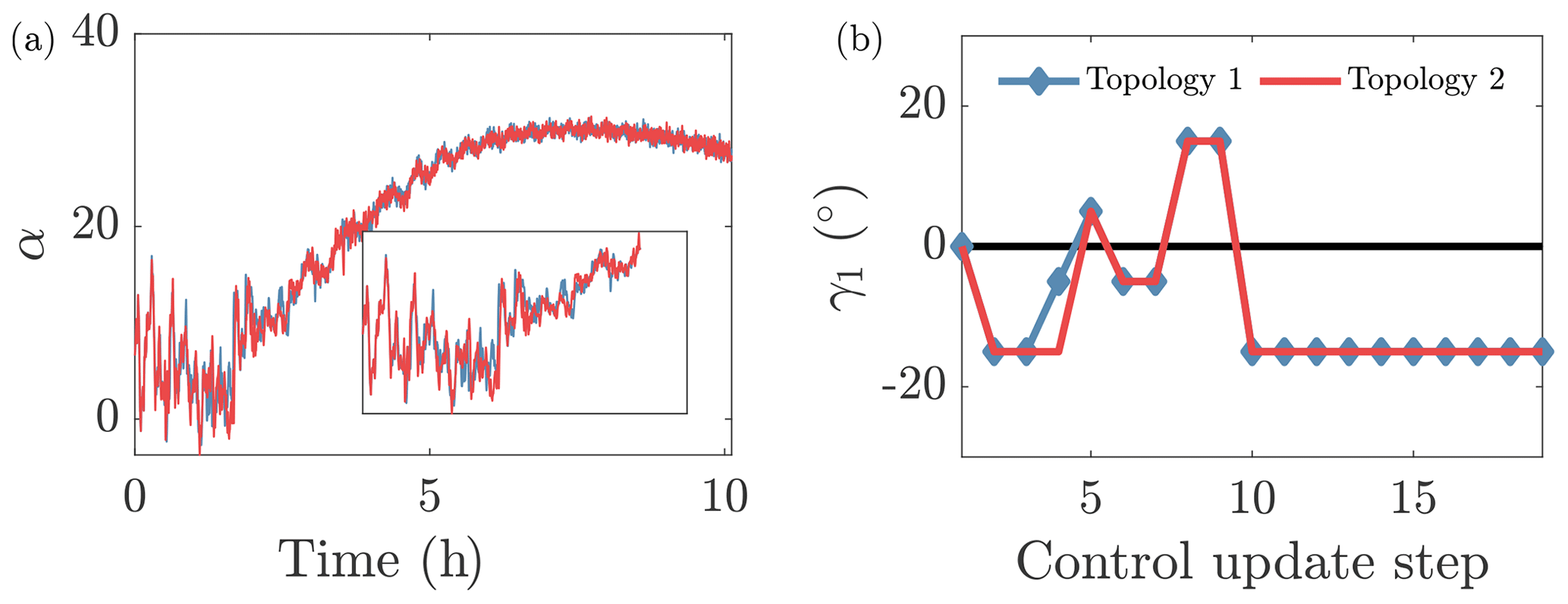
Figure D1(a) Reference turbine wind direction for open-loop wake steering control cases for two differing parallel processor topologies. The simulations are executed from identical initial conditions. (b) The yaw misalignment set points implemented in the two open-loop lookup table control cases.
The yaw misalignment lookup table synthesis is described in this section. The wake model presented in Part 1 (Howland et al., 2020c) is used for yaw set-point optimization for the eight wind turbines of interest (Fig. 1) for the wind directions encountered in the LES case, between (Fig. 2a). The wake spreading rate is prescribed using the empirical fit of Niayifar and Porté-Agel (2016), , where TI is the streamwise turbulence intensity. The proportionality constant of the presumed Gaussian wake is set to σ0=0.25 (Shapiro et al., 2019; Howland et al., 2020c). The parameter k* in the empirical fit of Niayifar and Porté-Agel (2016) is not identical to the parameter kw used in the lifting line wake model (Shapiro et al., 2018). An empirical calibration for kw is not available in the literature. Instead, the wake spreading rate kw is found by equating the Gaussian wake model form used by Niayifar and Porté-Agel (2016) with the form used in this study. The resulting empirical kw is
where x is the streamwise distance between the turbines normalized by the rotor diameter, CT is the coefficient of thrust, and k* is defined in the relationship above.
Figure E1Yaw misalignment set-point lookup table for open-loop control for turbines 1, 2, and 3 as a function of the incident wind direction.
The yaw set-point lookup table is constructed with a wind direction discretization of . The turbulence intensity is extracted from the baseline yaw-aligned control simulation as a function of time. The mean turbulence intensity in each wind direction bin (see Fig. 2c) is used to estimate the wake spreading rate k*, which is then used to compute kw in Eq. (E1). The yaw set points are then optimized in each wind direction bin for the prescribed kw and σ0. The resulting yaw set points for turbines 1, 2, and 3 are shown in Fig. E1. The other yaw misalignments are not shown for brevity but are provided in the dataset accompanying this study. The yaw misalignments are applied to the wind farm by selecting the closest wind direction bin to the moving average filtered wind direction estimate (see Fig. 11).
All data and computer code used in this paper are open source. The data and code are available at https://doi.org/10.5281/zenodo.5160943 (Howland, 2021a). The code is open source and available at https://github.com/FPAL-Stanford-University/PadeOps (Ghate et al., 2018).
MFH and JOD conceived the work. ASG and MFH developed the LES code. SKL supervised and obtained funding for LES code development. MFH conducted the analysis. MFH, JBQ, JJPM, WZ, and FPL contributed to control algorithm development. MFH wrote the manuscript. All authors contributed to edits.
The contact author has declared that neither they nor their co-authors have any competing interests.
Publisher’s note: Copernicus Publications remains neutral with regard to jurisdictional claims in published maps and institutional affiliations.
Aditya S. Ghate was funded by Tomkat Center for Sustainable Energy at Stanford University. Sanjiva K. Lele acknowledges partial support from NSF-CBET-1803378. The authors would also like to thank the referees and the associate editor for their thoughtful comments and contribution to this work.
This research has been supported by the National Science Foundation, Directorate for Engineering (grant no. NSF-CBET-1803378). Michael F. Howland was partially supported by Siemens Gamesa Renewable Energy. All simulations were performed on Stampede2 supercomputer under the XSEDE project ATM170028.
This paper was edited by Katherine Dykes and reviewed by Bart M. Doekemeijer and Paul van der Laan.
Abkar, M. and Porté-Agel, F.: Influence of atmospheric stability on wind-turbine wakes: A large-eddy simulation study, Phys. Fluids, 27, 035104, https://doi.org/10.1063/1.4913695, 2015. a, b, c
Abkar, M., Sharifi, A., and Porté-Agel, F.: Wake flow in a wind farm during a diurnal cycle, J. Turbul., 17, 420–441, 2016. a, b
Allaerts, D. and Meyers, J.: Large eddy simulation of a large wind-turbine array in a conventionally neutral atmospheric boundary layer, Phys. Fluids, 27, 065108, https://doi.org/10.1063/1.4922339, 2015. a
Annoni, J., Bay, C., Johnson, K., Dall'Anese, E., Quon, E., Kemper, T., and Fleming, P.: Wind direction estimation using SCADA data with consensus-based optimization, Wind Energ. Sci., 4, 355–368, https://doi.org/10.5194/wes-4-355-2019, 2019. a
Atkinson, B. and Wu Zhang, J.: Mesoscale shallow convection in the atmosphere, Rev. Geophys., 34, 403–431, 1996. a
Barthelmie, R. J. and Jensen, L.: Evaluation of wind farm efficiency and wind turbine wakes at the Nysted offshore wind farm, Wind Energy, 13, 573–586, 2010. a
Basu, S., Holtslag, A. A., Van De Wiel, B. J., Moene, A. F., and Steeneveld, G.-J.: An inconvenient “truth” about using sensible heat flux as a surface boundary condition in models under stably stratified regimes, Acta Geophys., 56, 88–99, 2008a. a
Basu, S., Vinuesa, J.-F., and Swift, A.: Dynamic LES modeling of a diurnal cycle, J. Appl. Meteorol. Clim., 47, 1156–1174, 2008b. a
Beare, R. J., Macvean, M. K., Holtslag, A. A., Cuxart, J., Esau, I., Golaz, J. C., Jimenez, M. A., Khairoutdinov, M., Kosovic, B., Lewellen, D., and Lund, T. S.: An intercomparison of large-eddy simulations of the stable boundary layer, Bound.-Lay. Meteorol., 118, 247–272, 2006. a
Bosveld, F. C., Baas, P., van Meijgaard, E., de Bruijn, E. I., Steeneveld, G.-J., and Holtslag, A. A.: The third GABLS intercomparison case for evaluation studies of boundary-layer models. Part A: Case selection and set-up, Bound.-Lay. Meteorol., 152, 133–156, 2014. a
Campagnolo, F. and Bottasso, C. L.: On the effectiveness of one-sided wake steering-A wind tunnel study with dynamic direction changes, in: 2021 American Control Conference (ACC), IEEE, 25–28 May 2021, New Orleans, LA, USA, 20942388, 3070–3075, https://doi.org/10.23919/ACC50511.2021.9483266, 2021. a
Campagnolo, F., Weber, R., Schreiber, J., and Bottasso, C. L.: Wind tunnel testing of wake steering with dynamic wind direction changes, Wind Energ. Sci., 5, 1273–1295, https://doi.org/10.5194/wes-5-1273-2020, 2020. a, b
Ciri, U., Rotea, M. A., and Leonardi, S.: Model-free control of wind farms: A comparative study between individual and coordinated extremum seeking, Renew. Energ., 113, 1033–1045, 2017. a
Deardorff, J. W.: Numerical investigation of neutral and unstable planetary boundary layers, J. Atmos. Sci., 29, 91–115, 1972. a
Doekemeijer, B. M., van der Hoek, D., and van Wingerden, J.-W.: Closed-loop model-based wind farm control using FLORIS under time-varying inflow conditions, Renew. Energ., 156, 719–730, 2020. a, b, c
Doekemeijer, B. M., Kern, S., Maturu, S., Kanev, S., Salbert, B., Schreiber, J., Campagnolo, F., Bottasso, C. L., Schuler, S., Wilts, F., Neumann, T., Potenza, G., Calabretta, F., Fioretti, F., and van Wingerden, J.-W.: Field experiment for open-loop yaw-based wake steering at a commercial onshore wind farm in Italy, Wind Energ. Sci., 6, 159–176, https://doi.org/10.5194/wes-6-159-2021, 2021. a, b
Evensen, G.: The ensemble Kalman filter: Theoretical formulation and practical implementation, Ocean Dynam., 53, 343–367, 2003. a
Fitch, A. C., Lundquist, J. K., and Olson, J. B.: Mesoscale influences of wind farms throughout a diurnal cycle, Mon. Weather Rev., 141, 2173–2198, 2013. a, b, c
Fleming, P., Scholbrock, A., Jehu, A., Davoust, S., Osler, E., Wright, A. D., and Clifton, A.: Field-test results using a nacelle-mounted lidar for improving wind turbine power capture by reducing yaw misalignment, J. Phys.-Conf. Ser., 524, 012002, https://doi.org/10.1088/1742-6596/524/1/012002, 2014. a, b
Fleming, P., King, J., Dykes, K., Simley, E., Roadman, J., Scholbrock, A., Murphy, P., Lundquist, J. K., Moriarty, P., Fleming, K., van Dam, J., Bay, C., Mudafort, R., Lopez, H., Skopek, J., Scott, M., Ryan, B., Guernsey, C., and Brake, D.: Initial results from a field campaign of wake steering applied at a commercial wind farm – Part 1, Wind Energ. Sci., 4, 273–285, https://doi.org/10.5194/wes-4-273-2019, 2019. a, b, c, d, e
Gadde, S. N. and Stevens, R. J.: Effect of low-level jet height on wind farm performance, J. Renew. Sustain. Ener., 13, 013305, https://doi.org/10.1063/5.0026232, 2021. a
Gebraad, P., Teeuwisse, F., Van Wingerden, J., Fleming, P. A., Ruben, S., Marden, J., and Pao, L.: Wind plant power optimization through yaw control using a parametric model for wake effects – a CFD simulation study, Wind Energy, 19, 95–114, 2016. a, b
Ghate, A.: Gabor mode enrichment in large eddy simulation of turbulent flows, PhD thesis, Stanford University, https://searchworks.stanford.edu/view/12797455 (last access: 5 August 2021), 2018. a, b
Ghate, A., Subramaniam, A., and Howland, M. F.: PadéOps, GitHub [code], available at: https://github.com/FPAL-Stanford-University/PadeOps (last access: 5 August 2021), 2018. a, b
Ghate, A. S. and Lele, S. K.: Subfilter-scale enrichment of planetary boundary layer large eddy simulation using discrete Fourier–Gabor modes, J. Fluid Mech., 819, 494–539, 2017. a
Horst, T., Kleissl, J., Lenschow, D., Meneveau, C., Moeng, C., Parlange, M., Sullivan, P., and Weil, J.: HATS: Field observations to obtain filtered fields from crosswind arrays of sonic anemometers in the atmospheric surface layer, J. Atmos. Sci, 61, 1566–1581, 2004. a
Howland, M. F.: Supporting data for Optimal closed-loop wake steering, Part 2: Diurnal cycle atmospheric boundary layer conditions, Zenodo [data set], https://doi.org/10.5281/zenodo.5160943, 2021a. a
Howland, M. F.: Wind farm yaw control set-point optimization under model parameter uncertainty, J. Renew. Sustain. Ener., 13, 043303, https://doi.org/10.1063/5.0051071, 2021b. a, b, c, d, e
Howland, M. F. and Dabiri, J. O.: Influence of Wake Model Superposition and Secondary Steering on Model-Based Wake Steering Control with SCADA Data Assimilation, Energies, 14, 52, https://doi.org/10.3390/en14010052, 2021. a, b, c, d
Howland, M. F., Lele, S. K., and Dabiri, J. O.: Wind farm power optimization through wake steering, P. Natl. Acad. Sci., 116, 14495–14500, 2019. a, b
Howland, M. F., Ghate, A. S., and Lele, S. K.: Coriolis effects within and trailing a large finite wind farm, in: AIAA Scitech 2020 Forum, 6–10 January 2020, Orlando, FL , p. 0994, https://doi.org/10.2514/6.2020-0994, 2020a. a
Howland, M. F., Ghate, A. S., and Lele, S. K.: Influence of the geostrophic wind direction on the atmospheric boundary layer flow, J. Fluid Mech., 883, A39, https://doi.org/10.1017/jfm.2019.889, 2020b. a, b, c
Howland, M. F., Ghate, A. S., Lele, S. K., and Dabiri, J. O.: Optimal closed-loop wake steering – Part 1: Conventionally neutral atmospheric boundary layer conditions, Wind Energ. Sci., 5, 1315–1338, https://doi.org/10.5194/wes-5-1315-2020, 2020c. a, b, c, d, e, f, g, h, i, j, k, l, m, n, o, p, q, r, s
Howland, M. F., González, C. M., Martínez, J. J. P., Quesada, J. B., Larranaga, F. P., Yadav, N. K., Chawla, J. S., and Dabiri, J. O.: Influence of atmospheric conditions on the power production of utility-scale wind turbines in yaw misalignment, J. Renew. Sustain. Ener., 12, 063307, https://doi.org/10.1063/5.0023746, 2020d. a, b, c, d, e, f, g, h
Hure, N., Turnar, R., Vašak, M., and Benčić, G.: Optimal wind turbine yaw control supported with very short-term wind predictions, in: 2015 IEEE International Conference on Industrial Technology (ICIT), IEEE, Seville, Spain, 17–19 March 2015, 15219611, 385–391, https://doi.org/10.1109/ICIT.2015.7125129, 2015. a
Iungo, G. V. and Porté-Agel, F.: Volumetric lidar scanning of wind turbine wakes under convective and neutral atmospheric stability regimes, J. Atmos. Ocean. Tech., 31, 2035–2048, 2014. a
Jensen, N. O.: A note on wind generator interaction, Vol. 2411, Roskilde, Denmark, Risø National Laboratory, 1983. a
Kanev, S.: Dynamic wake steering and its impact on wind farm power production and yaw actuator duty, Renew. Energ., 146, 9–15, 2020. a
Kumar, V., Kleissl, J., Meneveau, C., and Parlange, M. B.: Large-eddy simulation of a diurnal cycle of the atmospheric boundary layer: Atmospheric stability and scaling issues, Water Resour. Res., 42, W06D09, https://doi.org/10.1029/2005WR004651, 2006. a, b, c, d, e, f, g, h, i, j
Lele, S. K.: Compact finite difference schemes with spectral-like resolution, J. Comput. Phys., 103, 16–42, 1992. a
Liew, J., Urbán, A. M., and Andersen, S. J.: Analytical model for the power–yaw sensitivity of wind turbines operating in full wake, Wind Energ. Sci., 5, 427–437, https://doi.org/10.5194/wes-5-427-2020, 2020. a, b, c
Lissaman, P.: Energy effectiveness of arbitrary arrays of wind turbines, J. Energy, 3, 323–328, 1979. a
Macrí, S., Aubrun, S., Leroy, A., and Girard, N.: Experimental investigation of wind turbine wake and load dynamics during yaw maneuvers, Wind Energ. Sci., 6, 585–599, https://doi.org/10.5194/wes-6-585-2021, 2021. a
Martínez-Tossas, L. A., King, J., Quon, E., Bay, C. J., Mudafort, R., Hamilton, N., Howland, M. F., and Fleming, P. A.: The curled wake model: a three-dimensional and extremely fast steady-state wake solver for wind plant flows, Wind Energ. Sci., 6, 555–570, https://doi.org/10.5194/wes-6-555-2021, 2021. a
Muñoz-Esparza, D., Lundquist, J. K., Sauer, J. A., Kosović, B., and Linn, R. R.: Coupled mesoscale-LES modeling of a diurnal cycle during the CWEX-13 field campaign: From weather to boundary-layer eddies, J. Adv. Model. Earth Sy., 9, 1572–1594, 2017. a
Munters, W., Meneveau, C., and Meyers, J.: Turbulent inflow precursor method with time-varying direction for large-eddy simulations and applications to wind farms, Bound.-Lay. Meteorol., 159, 305–328, 2016. a
Niayifar, A. and Porté-Agel, F.: Analytical modeling of wind farms: A new approach for power prediction, Energies, 9, 741, https://doi.org/10.3390/en9090741, 2016. a, b, c, d, e, f
Nordström, J., Nordin, N., and Henningson, D.: The fringe region technique and the Fourier method used in the direct numerical simulation of spatially evolving viscous flows, SIAM J. Sci. Comput., 20, 1365–1393, 1999. a
Pope, S. B.: Turbulent flows, Cambridge University Press, 2001. a
Quick, J., Annoni, J., King, R., Dykes, K., Fleming, P., and Ning, A.: Optimization under uncertainty for wake steering strategies, J. Phys.-Conf. Ser., 854, 012036, https://doi.org/10.1088/1742-6596/854/1/012036, 2017. a, b, c
Quick, J., King, J., King, R. N., Hamlington, P. E., and Dykes, K.: Wake steering optimization under uncertainty, Wind Energ. Sci., 5, 413–426, https://doi.org/10.5194/wes-5-413-2020, 2020. a, b, c, d
Rott, A., Doekemeijer, B., Seifert, J. K., van Wingerden, J.-W., and Kühn, M.: Robust active wake control in consideration of wind direction variability and uncertainty, Wind Energ. Sci., 3, 869–882, https://doi.org/10.5194/wes-3-869-2018, 2018. a, b
Salesky, S. T., Chamecki, M., and Bou-Zeid, E.: On the nature of the transition between roll and cellular organization in the convective boundary layer, Bound.-Lay. Meteorol., 163, 41–68, 2017. a
Sanchez Gomez, M. and Lundquist, J. K.: The effect of wind direction shear on turbine performance in a wind farm in central Iowa, Wind Energ. Sci., 5, 125–139, https://doi.org/10.5194/wes-5-125-2020, 2020. a
Sanz Rodrigo, J., Chavez Arroyo, R. A., Moriarty, P., Churchfield, M., Kosović, B., Réthoré, P.-E., Hansen, K. S., Hahmann, A., Mirocha, J. D., and Rife, D.: Mesoscale to microscale wind farm flow modeling and evaluation, WIRES Energy Environ., 6, e214, https://doi.org/10.1002/wene.214, 2017a. a, b
Sanz Rodrigo, J., Churchfield, M., and Kosovic, B.: A methodology for the design and testing of atmospheric boundary layer models for wind energy applications, Wind Energ. Sci., 2, 35–54, https://doi.org/10.5194/wes-2-35-2017, 2017b. a
Schreiber, J., Bottasso, C. L., Salbert, B., and Campagnolo, F.: Improving wind farm flow models by learning from operational data, Wind Energ. Sci., 5, 647–673, https://doi.org/10.5194/wes-5-647-2020, 2020. a
Segalini, A. and Dahlberg, J.-Å.: Blockage effects in wind farms, Wind Energy, 23, 120–128, 2020. a
Shapiro, C. R., Gayme, D. F., and Meneveau, C.: Modelling yawed wind turbine wakes: a lifting line approach, J. Fluid Mech., 841, R1, https://doi.org/10.1017/jfm.2018.75, 2018. a
Shapiro, C. R., Starke, G. M., Meneveau, C., and Gayme, D. F.: A Wake Modeling Paradigm for Wind Farm Design and Control, Energies, 12, 2956, https://doi.org/10.3390/en12152956, 2019. a
Simley, E., Fleming, P., and King, J.: Design and analysis of a wake steering controller with wind direction variability, Wind Energ. Sci., 5, 451–468, https://doi.org/10.5194/wes-5-451-2020, 2020. a, b, c
Simley, E., Fleming, P., King, J., and Sinner, M.: Wake steering wind farm control with preview wind direction information, Tech. rep., National Renewable Energy Lab. (NREL), Golden, CO (United States), https://doi.org/10.23919/ACC50511.2021.9483008, 2021. a, b
Starke, G. M., Meneveau, C., King, J. R., and Gayme, D. F.: The area localized coupled model for analytical mean flow prediction in arbitrary wind farm geometries, J. Renew. Sustain. Ener., 13, 033305, https://doi.org/10.1063/5.0042573, 2021. a
Stull, R. B.: An introduction to boundary layer meteorology, vol. 13, Springer Science & Business Media, https://doi.org/10.1007/978-94-009-3027-8, 2012. a
Sullivan, P. P., Horst, T. W., Lenschow, D. H., Moeng, C.-H., and Weil, J. C.: Structure of subfilter-scale fluxes in the atmospheric surface layer with application to large-eddy simulation modelling, J. Fluid Mech., 482, 101–139, 2003. a
Sullivan, P. P., Weil, J. C., Patton, E. G., Jonker, H. J., and Mironov, D. V.: Turbulent winds and temperature fronts in large-eddy simulations of the stable atmospheric boundary layer, J. Atmos. Sci., 73, 1815–1840, 2016. a
Svensson, G. A. A. M. H., Holtslag, A. A. M., Kumar, V., Mauritsen, T., Steeneveld, G. J., Angevine, W. M., Bazile, E., Beljaars, A., De Bruijn, E. I. F., Cheng, A., and Conangla, L.: Evaluation of the diurnal cycle in the atmospheric boundary layer over land as represented by a variety of single-column models: The second GABLS experiment, Bound.-Lay. Meteorol., 140, 177–206, 2011. a
Thorpe, A. J. and Guymer, T. H.: The nocturnal jet, Quarterly Journal of the Royal Meteorological Society, 103, 633–653, 1977. a
van der Laan, M. P., Kelly, M., and Baungaard, M.: A pressure-driven atmospheric boundary layer model satisfying Rossby and Reynolds number similarity, Wind Energ. Sci., 6, 777–790, https://doi.org/10.5194/wes-6-777-2021, 2021. a
Van de Wiel, B. J., Moene, A., Steeneveld, G., Baas, P., Bosveld, F., and Holtslag, A.: A conceptual view on inertial oscillations and nocturnal low-level jets, J. Atmos. Sci., 67, 2679–2689, 2010. a
Van Wijk, A., Beljaars, A., Holtslag, A., and Turkenburg, W.: Evaluation of stability corrections in wind speed profiles over the North Sea, J. Wind Eng. Ind. Aerod., 33, 551–566, 1990. a
Wharton, S. and Lundquist, J. K.: Assessing atmospheric stability and its impacts on rotor-disk wind characteristics at an onshore wind farm, Wind Energy, 15, 525–546, 2012a. a
Wharton, S. and Lundquist, J. K.: Atmospheric stability affects wind turbine power collection, Environ. Res. Lett., 7, 014005, https://doi.org/10.1088/1748-9326/7/1/014005, 2012b. a
Wyngaard, J. C.: Turbulence in the Atmosphere, Cambridge University Press, https://doi.org/10.1017/CBO9780511840524, 2010. a, b
Zong, H. and Porté-Agel, F.: A momentum-conserving wake superposition method for wind farm power prediction, J. Fluid Mech., 889, A8, https://doi.org/10.1017/jfm.2020.77, 2020. a, b
- Abstract
- Introduction
- Model-based closed-loop wake steering control methodology updates
- Setup of large eddy simulations of the diurnal cycle
- Wake steering results
- Conclusions
- Appendix A: Statistical wind direction forecast algorithm
- Appendix B: Idealized diurnal cycle setup
- Appendix C: Diurnal cycle validation
- Appendix D: Note on wake steering LES initialization
- Appendix E: Lookup table synthesis
- Code and data availability
- Author contributions
- Competing interests
- Disclaimer
- Acknowledgements
- Financial support
- Review statement
- References