Applying a random time mapping to Mann-modeled turbulence for the generation of intermittent wind fields

A new approach to derive a synthetic wind field model which combines spatial correlations from the Mann model and intermittency is introduced. The term intermittency describes the transition from Gaussian to non-Gaussian velocity increment statistics at small scales, where non-Gaussian velocity increment statistics imply a higher probability for extreme values than a Gaussian distribution. The presented new model is named the Time-mapped Mann model. The intermittency is introduced by applying a special random time-mapping procedure to the regular Mann model. The time-mapping procedure is based on the so-called continuous-time random walk model. As will be shown, the new Time-mapped Mann field reflects spatial correlations from the Mann model in the plane perpendicular to flow direction and temporal intermittency. In the first wind turbine study, the new Time-mapped Mann field and a regular Mann field are used as inflow to a wind turbine in a blade element momentum simulation. It is shown that the wind field intermittency carries over to loads of the wind turbine and, thus, shows the importance of carefully modeling synthetic wind fields.

1 Introduction

Wind energy plays a leading role in the energy transition process to renewable energy these days. In 2020, the world witnessed new wind energy installations of 93 GW, making the global installed capacity of wind energy 743 GW according to the Global Wind Energy Council (GWEC, 2021). The growing demand for wind energy resulted in growing turbine rotor diameters. This leads to an increase in loads on the different turbine components like blades and tower. Numerical simulations are now crucial to predict loads and performance parameters in the early design stages. In this context, wind fields should be accurately simulated to be able to anticipate extreme load cases and fatigue loads on different parts of the wind turbine to reach the optimum design without compromising the structural limits of these components. However, the physics of the turbulent wind fields are not yet completely understood, and many models were proposed to simulate these fields as described in the following.

The IEC 61400-1 standard for wind turbines (Han, 2007) recommends using Gaussian-based atmospheric turbulence models, namely Kaimal (Kaimal et al., 1972) and Mann (Mann, 1994, 1998) models, to simulate turbulent wind fields. These two turbulent wind field models imply the assumption that the velocity increments of the wind fields behave in a Gaussian manner.

However, it is well documented that the velocity increments of real atmospheric wind fields show non-Gaussian behavior, which is widely called intermittency. Through the heavy tails of the distribution, this implies a larger probability for extreme values than in a Gaussian distribution. Boettcher et al. (2003) showed that wind field measurements from near the German North Sea coastline have a non-Gaussian distribution of two-point statistics of velocity increments for certain mean wind velocity intervals. Also, Vindel et al. (2008) have shown the intermittency of velocity increment statistics in data of the atmospheric boundary layer velocity measured by Cuxart et al. (2000). More recent research like the work of Liu et al. (2010) and Mücke et al. (2011) reached the same conclusion. This means that extreme wind velocity increments happen more often than what is predicted using the turbulence models recommended by the IEC standard. Also, Morales et al. (2012) presented a statistical scheme to assess turbulent wind fields that uses both lower- and higher-order one-point and two-point statistics. They have also compared synthetic turbulent time series using the Kaimal model with atmospheric turbulent wind field measurements from the research platform FINO-1. They have shown that the synthetic fields generated with the Kaimal model failed to grasp the intermittent behavior of the wind field.

The questions that arise at this point are the following: how can a synthetic wind field be modeled as realistically as possible and how is this reflected in the turbine loads? In this direction, Kleinhans (2008) proposed a new approach to generate an intermittent wind field using the continuous-time random walk (CTRW) theory. This approach is based on stochastic differential equations and a function that maps from an intrinsic time to real time to generate such an intermittent field, whereas the spatial correlations are not as realistic as in the Mann field. A brief description of the CTRW model will be introduced in Sect. 2.3. In addition to the CTRW model, there also exist other models which can be applied to generate synthetic wind fields with intermittent features, e.g., by Friedrich et al. (2021) based on multi-point statistics which are not further discussed here.

Gontier et al. (2007) compared the effect of the intermittent CTRW wind field and other standard turbulence models (Kaimal and von Kármán, 1948) on the fatigue loads of the D8 small wind turbine at different wind speeds. The authors have found that the simulated wind turbine loads in the case of using the CTRW wind model show heavy-tailed second-order statistics, while the loads simulated by using the other two models do not show such a behavior. However, the authors could not give definitive conclusions regarding the peak loads from their simulations. Later, Mücke et al. (2011) compared the statistics of wind fields generated by the Kaimal model, intermittent wind fields generated using CTRW, and the atmospheric wind data measured within the GROWIAN project (Körber et al., 1988). The three cases were then used in the NREL FAST (V6.01) (Jonkman and Jonkman, 2005) blade element momentum (BEM) simulator to model the resulting rotor torque of the 1.5 MW WindPACT (Malcolm and Hansen, 2006) turbine. Also, the authors analyzed the stress cycles for the rotor torque time series to study the effects of the three wind fields on fatigue loads. They have concluded that the statistics of the numerical results using the Kaimal wind field qualitatively differ from the results obtained from measurements. On the other hand, they have concluded that the synthetic wind field generated by the CTRW managed to reproduce the intermittency at small timescales. Also, the CTRW field managed to qualitatively provide intermittent rotor torque statistics like the resulting torque from measurements.

Gong and Chen (2014) numerically investigated the short- and long-term extreme responses of the onshore NREL 5 MW turbine for a Gaussian wind field using a Kaimal wind spectrum and a second non-Gaussian wind field generated by a translation process theory introduced by Gioffre et al. (2000). They showed that the non-Gaussian wind field resulted in larger extreme loads of the blade root edgewise and tower fore–aft moments while the responses of a stand-still wind turbine case were less sensitive to the non-Gaussianity of the wind field. Schottler et al. (2017) applied an intermittent wind field on a 0.58 m diameter model wind turbine in a wind tunnel to measure the effect of such a wind field on the thrust, power, and torque on the rotor. The authors found out that the turbine did not smooth out the intermittency, and they also concluded that assuming non-Gaussian wind fields may lead to significant differences in loads on the turbine.

Schwarz et al. (2018, 2019) isolated and investigated the effect of intermittent wind velocity on equivalent fatigue loads of the NREL 5 MW wind turbine at different wind speeds using BEM simulations. To isolate the effects of intermittency, two different velocity fields were generated utilizing the CTRW model: a Gaussian and a non-Gaussian wind field. Both of them have the same features except for the intermittency that was introduced in the non-Gaussian field utilizing the time mapping, which was simply omitted in the Gaussian case. For the two wind cases, three different spatial correlations were investigated: fully correlated fields, delta-correlated fields, and 3×3 sub-divided fully correlated fields. After analyzing the results of the different cases, the authors noticed that the highest effect of intermittency of the wind fields on the loads can be observed in the fully correlated case with a 5 % to 10 % increase in fatigue loads while it completely disappears in the delta-correlated field. For the 3×3 sub-divided fully correlated field, intermittent loads were ranged between the other two cases. The authors concluded that intermittency in the wind field had a significant effect on loads.

Berg et al. (2016) also compared Gaussian and non-Gaussian wind fields using large eddy simulations (LESs) in the HAWC2 computational fluid dynamics (CFD) software (Larsen and Hansen, 2007). They studied the effect of the intermittency on the different blade, tower, and shaft loads and deflections of the NREL 5 MW wind turbine. In contrast with the aforementioned studies, they concluded that intermittency has no significant effect on the studied parameters. This shows that even though many studies reveal the influence of intermittency, the effect needs further investigation. Recently, Bangga and Lutz (2021) simulated the DANAERO 2 MW wind turbine under turbulent inflow using CFD and BEM simulations. In their work, they have compared tip deflections, flapwise and edgewise loads on the blade root, and the damage equivalent load (DEL) of the DANAERO wind turbine affected by a synthetic turbulent Mann field. The results of the simulated loads and deflections in their research have shown good agreement with measured data from the turbine operating under the same conditions. Specifically, the authors compared the flapwise, edgewise, and torsional deflections' spectra of the turbine under laminar and turbulent inflows. The presented analysis of the spectra is very detailed. However, the spectra of the deflections are not enough to study all aspects of the effects of turbulence.

In the present paper, a novel method to numerically generate a synthetic, intermittent turbulent wind field is introduced. Within this new method, the time-mapping technique introduced by Kleinhans (2008) is applied on a turbulent wind field generated by the Mann model. A detailed comparison between our new wind field using this time-mapping technique, referred to as the Time-mapped Mann field in the following, and a standard Mann-modeled wind field is carried out. As will be shown, the advantage of the new Time-mapped Mann field is that it combines spatial correlations from the Mann wind field and intermittent behavior. Also, a first insightful comparison between selected mechanical loads on a 1.5 MW wind turbine resulting from both the Time-mapped Mann field and the standard Mann field is illustrated. The analysis of these turbine loads reveals the effect of intermittency on wind turbine loads.

2 Scientific background on synthetic wind fields

Before illustrating the derivation of the new Time-mapped Mann field, general wind field statistics that will be used to analyze the generated wind fields are introduced in Sect. 2.1. After that, in Sect. 2.2 and 2.3 the Mann and CTRW turbulent wind field models are introduced. The main purpose of this section is to provide the theoretical background for the derivation of the new model and its analysis. This chapter is also intended to be self-contained and provide all the necessary equations for the introduction of the proposed new Time-mapped Mann model.

2.1 Statistics of wind fields

For any turbulent wind field, the wind velocity time series U_i can be expressed as a function of mean velocity 〈U_i〉 and velocity fluctuation u_i, with $i=\mathrm{1},\mathrm{2},\mathrm{3}$ in three-dimensional space:

$$\begin{array}{}\text{(1)}& U_i=\langle U_i\rangle +u_i,\end{array}$$

where the angular brackets 〈.〉 denote an ensemble average. Throughout this paper, the ensemble average is partly replaced by spatial or temporal averages for practical purposes which will be indicated in the respective cases below. In our case, we assume only a mean velocity in the x₁ direction, i.e., $\langle \mathit{U}\rangle =(\langle U_{\mathrm{1}}\rangle ,\mathrm{0},\mathrm{0})$, which is the inflow direction in the following. From this decomposition, the turbulence intensity (TI) can be calculated as follows:

$$\begin{array}{}\text{(2)}& {\mathrm{TI}}_i={\displaystyle \frac{{\mathit{\sigma }}_i}{\langle U_{\mathrm{1}}\rangle }}={\displaystyle \frac{\sqrt{\langle u_i^{\mathrm{2}}\rangle }}{\langle U_{\mathrm{1}}\rangle }},\end{array}$$

where i indicates the direction in which the turbulence intensity is calculated with respect to the mean velocity in the inflow component 〈U₁〉 and σ_i is the variance of u_i. The turbulence intensity is a one-point statistics in space and time of wind fields. However, for information on the spatial structures, one-point statistics is not sufficient and two-point statistics should be used for more information about the wind fields. As an example, the co-variance tensor contains two-point statistics:

$$\begin{array}{}\text{(3)}& R_{ij}(\mathbf{r},\mathbf{x},t)=\langle u_i(\mathbf{x},t)u_j(\mathbf{x}+\mathbf{r},t)\rangle ,\end{array}$$

where R_ij is the two-point correlation which is independent of the position x in the case of homogeneous turbulence and r is the displacement vector between the two points. Since Eq. (3) is a theoretical equation, there are no restrictions on selecting the two points for the two-point statistics. However, in practice, it is limited to the size of the data set of the wind fields. The spectral velocity tensor for homogeneous turbulence resulting from a Fourier transform of Eq. (3) gives (Pope, 2001)

$$\begin{array}{}\text{(4)}& {\mathrm{\Phi }}_{ij}(\mathit{\kappa },t)={\displaystyle \frac{\mathrm{1}}{(\mathrm{2}\mathit{\pi }{)}^{\mathrm{3}}}}\underset{-\mathrm{\infty }}{\overset{\mathrm{\infty }}{\int }}\underset{-\mathrm{\infty }}{\overset{\mathrm{\infty }}{\int }}\underset{-\mathrm{\infty }}{\overset{\mathrm{\infty }}{\int }}{R}_{ij}(\mathbf{r},t)\exp (-\mathrm{i}\mathit{\kappa }\cdot \mathbf{r})\mathrm{d}\mathbf{r}.\end{array}$$

In this equation, $\mathit{\kappa }=({\mathit{\kappa }}_{\mathrm{1}},{\mathit{\kappa }}_{\mathrm{2}},{\mathit{\kappa }}_{\mathrm{3}})$ represents a three-dimensional wavenumber vector for the three directions. The one-dimensional spectrum follows from Eq. (4) by integration:

$$\begin{array}{}\text{(5)}& \begin{array}{rl}{F}_i({\mathit{\kappa }}_{\mathrm{1}},t)& =\underset{-\mathrm{\infty }}{\overset{\mathrm{\infty }}{\int }}\underset{-\mathrm{\infty }}{\overset{\mathrm{\infty }}{\int }}{\mathrm{\Phi }}_{ii}(\mathit{\kappa },t)\mathrm{d}{\mathit{\kappa }}_{\mathrm{2}}\mathrm{d}{\mathit{\kappa }}_{\mathrm{3}}\\ & ={\displaystyle \frac{\mathrm{1}}{\mathrm{2}\mathit{\pi }}}\underset{-\mathrm{\infty }}{\overset{\mathrm{\infty }}{\int }}{R}_{ii}(r_{\mathrm{1}},\mathrm{0},\mathrm{0},t)\exp (-\mathrm{i}{\mathit{\kappa }}_{\mathrm{1}}{r}_{\mathrm{1}})\mathrm{d}{r}_{\mathrm{1}},\end{array}\end{array}$$

where the ii index refers to the respective diagonal element of the tensor. The one-dimensional spectra with respect to κ₂ and κ₃ are computed accordingly. The spectral coherence for the wavenumber κ₁ with respect to two separate points in the x₂−x₃ plane reads (Mann, 1994)

$$\begin{array}{}\text{(6)}& {\mathrm{coh}}_{ij}({\mathit{\kappa }}_{\mathrm{1}},\mathrm{\Delta }{x}_{\mathrm{2}},\mathrm{\Delta }{x}_{\mathrm{3}},t)\equiv {\displaystyle \frac{\left|{\mathit{\chi }}_{ij}\right({\mathit{\kappa }}_{\mathrm{1}},\mathrm{\Delta }{x}_{\mathrm{2}},\mathrm{\Delta }{x}_{\mathrm{3}},t){|}^{\mathrm{2}}}{F_i({\mathit{\kappa }}_{\mathrm{1}},t)F_j({\mathit{\kappa }}_{\mathrm{1}},t)}},\end{array}$$

with F_i(κ₁,t) from Eq. (5) and the cross spectra χ_ij as defined below:

$$\begin{array}{}\text{(7)}& {\displaystyle }\begin{array}{rl}{\mathit{\chi }}_{ij}& ({\mathit{\kappa }}_{\mathrm{1}},\mathrm{\Delta }{x}_{\mathrm{2}},\mathrm{\Delta }{x}_{\mathrm{3}},t)\\ & ={\displaystyle \frac{\mathrm{1}}{\mathrm{2}\mathit{\pi }}}\underset{-\mathrm{\infty }}{\overset{\mathrm{\infty }}{\int }}{R}_{ij}(r_{\mathrm{1}},\mathrm{\Delta }{x}_{\mathrm{2}},\mathrm{\Delta }{x}_{\mathrm{3}})\exp (-\mathrm{i}{\mathit{\kappa }}_{\mathrm{1}}{r}_{\mathrm{1}})\mathrm{d}{r}_{\mathrm{1}}\end{array}\text{(8)}& {\displaystyle }=\underset{-\mathrm{\infty }}{\overset{\mathrm{\infty }}{\int }}\underset{-\mathrm{\infty }}{\overset{\mathrm{\infty }}{\int }}{\mathrm{\Phi }}_{ij}(\mathit{\kappa },t)\exp \left(\mathrm{i}\right({\mathit{\kappa }}_{\mathrm{2}}\mathrm{\Delta }{x}_{\mathrm{2}}+{\mathit{\kappa }}_{\mathrm{3}}\mathrm{\Delta }{x}_{\mathrm{3}}\left)\right)\mathrm{d}{\mathit{\kappa }}_{\mathrm{2}}\mathrm{d}{\mathit{\kappa }}_{\mathrm{3}},\end{array}$$

where Δx indicates the spatial step in three-dimensional space with its components Δx₁, Δx₂, and Δx₃ in the x₁, x₂, and x₃ directions, respectively. Another example of two-point statistics is the increment statistics in space described by

$$\begin{array}{}\text{(9)}& {\stackrel{\mathrm{̃}}{v}}_i(\mathbf{x},\mathrm{\Delta }\mathbf{x},t)=u_i(\mathbf{x}+\mathrm{\Delta }\mathbf{x},t)-u_i(\mathbf{x},t).\end{array}$$

Instead of spatial increments, one can also consider temporal increments as

$$\begin{array}{}\text{(10)}& v_i(\mathbf{x},t,\mathit{\tau })=u_i(\mathbf{x},t+\mathit{\tau })-u_i(\mathbf{x},t),\end{array}$$

where τ indicates the time lag. The probability density functions (PDFs) of the introduced temporal increments v_i have been investigated (Vindel et al., 2008; Liu et al., 2010; Mücke et al., 2011; Böttcher et al., 2007; Muzy et al., 2010) as part of a more detailed characterization of wind turbulence beyond the standard guidelines. The Gaussian distribution is completely described by the mean and the variance. Further statistical information is required for characterizing a non-Gaussian distribution. The so-called kurtosis of a distribution allows quantification of its deviation from a Gaussian distribution. For the temporal increments v_i, the kurtosis is defined as

$$\begin{array}{}\text{(11)}& \text{Kurt}\left(v_i\right)(\mathbf{x},t,\mathit{\tau })={\displaystyle \frac{\langle v_i(\mathbf{x},t,\mathit{\tau }{)}^{\mathrm{4}}\rangle }{\langle v_i(\mathbf{x},t,\mathit{\tau }{)}^{\mathrm{2}}{\rangle }^{\mathrm{2}}}}.\end{array}$$

For a Gaussian distribution, the kurtosis equals 3. Higher values indicate a heavy-tailed distribution in which extreme velocity increment values have a higher probability than predicted by a Gaussian distribution. We assume statistically stationary turbulence and, hence, omit the time t in the equations in the following.

Figure 1 shows characteristics of temporal velocity increment statistics of atmospheric wind speed measurements. The data were collected at the site of a Nordex wind turbine, located in northern Germany. The wind sensor was mounted at a height of 125 m. Time series of 10 min in length were considered for the analysis. These time series correspond to the horizontal magnitude of the wind speed measured at the hub height with a sampling rate of 50 Hz; the vertical component (U₃) was neglected here. In total, 494 time series were provided. Similar to Eq. (1), the measured wind speed can be decomposed as $U_{\mathrm{meas}}=\langle U_{\mathrm{meas}}\rangle +u_{\mathrm{meas}}$, where 〈U_meas〉 is calculated over the 10 min period. The turbulence intensity for the measured data is calculated as TI${}_{\mathrm{meas}}=\sqrt{\langle u_{\mathrm{meas}}^{\mathrm{2}}\rangle }/\langle U_{\mathrm{meas}}\rangle$. All the mean values of the wind direction, calculated over each of the 10 min periods, are distributed within a range of 165^∘. The selection and preparation of the data set were performed by Nordex according to internal objectives from the analysis. Here, we used the wind data set for illustration purposes rather than for a rigorous investigation of its characterization. Nevertheless, for our study, we investigate the time series of the wind velocity with similar first- and second-order moments. Accordingly, we selected a subset of time series whose values of mean wind speed and turbulence intensity are contained within a specific range. The range is defined as 9±1 m s⁻¹ for the mean wind speed and 0.15±0.02 for the turbulence intensity. Further, we also constrain the data in terms of their wind direction. For that, we consider the mean direction calculated over the 10 min period. Then, we define a range of ±20^∘ from the main wind direction at the specific site. After the selection process, 20 out of the 497 available time series are analyzed.

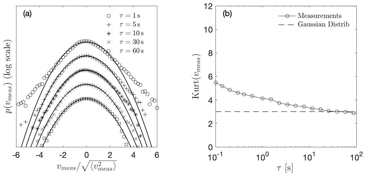
Figure 1 Statistical description of turbulent wind measurements from a Nordex wind turbine located in northern Germany. (a) Normalized PDFs of velocity increments v_meas for different values of τ. The distributions for different values of τ, increasing from top to bottom, are depicted by different markers. In addition, solid lines correspond to Gaussian distributions with identical mean and standard deviation. In principle, the curves would all lie on top of each other, but here the curves are shifted vertically for better visualization. (b) Kurtosis of velocity increments v_meas as a function of τ. The angular brackets denote moving averages within the individual 600 s time series and then over all data sets.

The increments for the atmospheric measured data $v_{\mathrm{meas}}=u_{\mathrm{meas}}(\mathrm{x},t+\mathit{\tau })-u_{\mathrm{meas}}(\mathrm{x},t)$ were calculated similar to Eq. (10). Then, the statistics of v_meas are computed for the whole subset of 20 conditioned 10 min time series. Figure 1a presents the PDFs of v_meas for different time lags τ from 1 to 60 s. For clarity of presentation, individual distributions are depicted with different markers and shifted vertically. For comparison, all the PDFs are normalized to a standard deviation equal to 1, and the corresponding Gaussian distributions are shown by a solid line.

As can be observed, the PDFs of v_meas for timescales τ equal to 1, 5, and 10 s deviate from the respective Gaussian distributions. Specifically, the distributions of v_meas show heavy tails which represent the high probability of extreme events, which is higher than for the Gaussian PDFs. This effect, which is called intermittency, is a well-known feature of atmospheric wind as Vindel et al. (2008), Liu et al. (2010), Mücke et al. (2011), and Böttcher et al. (2007) and many others have found. Similar to the results from the investigations mentioned earlier, Fig. 1a shows that the temporal increments v_meas are intermittent over a broad range of time lags τ. The evolution of the intermittency with τ can be quantified from the kurtosis. Figure 1b shows the calculated kurtosis of the PDFs according to Eq. (11) of the atmospheric increments v_meas as a function of τ. The values of Kurt(v_meas) higher than 3 reveal the intermittent behavior of the atmospheric data over a wide range of τ. For the analyzed data, intermittent features are distinguishable up to timescales of τ≈11 s when Kurt(v_meas) converges to the Gaussian value of 3.

2.2 Mann model

The basis of the Mann model (Mann, 1994, 1998) is a properly modeled spectral tensor according to Eq. (4). In this model, the turbulent velocity field is assumed to be incompressible, and the velocity fluctuations are assumed to be homogeneous in space. The resulting velocity field depends on only three parameters, namely a length scale L; a non-dimensional parameter Γ, which is related to the eddy lifetime and, hence, to the shear gradient; and a parameter $c_K{\mathit{ϵ}}^{\mathrm{2}/\mathrm{3}}$ with c_K as a constant and ϵ as the turbulent dissipation rate per unit mass. Within these assumptions, the second-order statistics such as variances and cross spectra of real wind can be met. In the case of isotropic turbulence (where assuming no shear), the spectral tensor takes the form (Pope, 2001)

$$\begin{array}{}\text{(12)}& {\mathrm{\Phi }}_{ij}^{\mathrm{iso}}\left(\mathit{\kappa }\right)={\displaystyle \frac{E\left(\mathit{\kappa }\right)}{\mathrm{4}\mathit{\pi }{\mathit{\kappa }}^{\mathrm{4}}}}({\mathit{\delta }}_{ij}{\mathit{\kappa }}^{\mathrm{2}}-{\mathit{\kappa }}_i{\mathit{\kappa }}_j),\end{array}$$

with κ as the magnitude of κ and E(κ) as the energy spectrum. E(κ) can be expressed with $c_K{\mathit{ϵ}}^{\mathrm{2}/\mathrm{3}}$ and L that leads to (von Kármán, 1948; Pope, 2001)

$$\begin{array}{}\text{(13)}& {\mathrm{\Phi }}_{ij}^{\mathrm{iso}}\left(\mathit{\kappa }\right)={\displaystyle \frac{c_K{\mathit{ϵ}}^{\mathrm{2}/\mathrm{3}}{L}^{\mathrm{17}/\mathrm{3}}}{\mathrm{4}\mathit{\pi }}}{\displaystyle \frac{{\mathit{\delta }}_{ij}{\mathit{\kappa }}^{\mathrm{2}}-{\mathit{\kappa }}_i{\mathit{\kappa }}_j}{[\mathrm{1}+(L\mathit{\kappa }{)}^{\mathrm{2}}{]}^{\mathrm{17}/\mathrm{6}}}}.\end{array}$$

The corresponding one-dimensional spectra result in Mann (1994):

$$\begin{array}{}\text{(14)}& F_i\left({\mathit{\kappa }}_{\mathrm{1}}\right)=\mathit{\{}\begin{array}{ll}\frac{\mathrm{9}}{\mathrm{55}}{c}_{\mathrm{K}}{\mathit{\epsilon }}^{\mathrm{2}/\mathrm{3}}\frac{\mathrm{1}}{(L^{-\mathrm{2}}+{\mathit{\kappa }}_{\mathrm{1}}^{\mathrm{2}}{)}^{\mathrm{5}/\mathrm{6}}}& \mathrm{for}i=\mathrm{1}\\ \frac{\mathrm{3}}{\mathrm{110}}{c}_{\mathrm{K}}{\mathit{\epsilon }}^{\mathrm{2}/\mathrm{3}}\frac{\mathrm{3}{L}^{-\mathrm{2}}+\mathrm{8}{\mathit{\kappa }}_{\mathrm{1}}^{\mathrm{2}}}{(L^{-\mathrm{2}}+{\mathit{\kappa }}_{\mathrm{1}}^{\mathrm{2}}{)}^{\mathrm{11}/\mathrm{6}}}& \mathrm{for}i\in \mathit{\{}\mathrm{2},\mathrm{3}\mathit{\}},\end{array}\end{array}$$

and, accordingly, the variance becomes

$$\begin{array}{}\text{(15)}& \begin{array}{rl}{\mathit{\sigma }}_{iso}^{\mathrm{2}}& ={\mathit{\sigma }}_{\mathrm{1}}^{\mathrm{2}}={\mathit{\sigma }}_{\mathrm{2}}^{\mathrm{2}}={\mathit{\sigma }}_{\mathrm{3}}^{\mathrm{2}}={\displaystyle \frac{\mathrm{9}}{\mathrm{55}}}{\displaystyle \frac{\sqrt{\mathit{\pi }}\mathrm{\Gamma }\left(\frac{\mathrm{1}}{\mathrm{3}}\right)}{\mathrm{\Gamma }\left(\frac{\mathrm{5}}{\mathrm{6}}\right)}}{c}_K{\mathit{ϵ}}^{\mathrm{2}/\mathrm{3}}{L}^{\mathrm{2}/\mathrm{3}}\\ & \approx \mathrm{0.688}{c}_{\mathrm{K}}{\mathit{ϵ}}^{\mathrm{2}/\mathrm{3}}{L}^{\mathrm{2}/\mathrm{3}},\end{array}\end{array}$$

where in this equation the Γ denotes the mathematical Gamma function. The value of the $c_K{\mathit{ϵ}}^{\mathrm{2}/\mathrm{3}}$ parameter can be found by fitting the model to specific site data assuming isotropic turbulence and an infinitely large domain. Another possible way to avoid such assumptions was suggested by Larsen and Hansen (2007), who suggest choosing the value of $c_K{\mathit{ϵ}}^{\mathrm{2}/\mathrm{3}}$ arbitrarily and then re-scaling the velocity field with a scaling factor. The value of $c_K{\mathit{ϵ}}^{\mathrm{2}/\mathrm{3}}$ was taken according to the Engineering Sciences Data Unit (ESDU, 1982) spectral model to achieve TI₁≈10 % as will be explained later in detail.

The Mann model provides a spatially correlated synthetic turbulent wind field where spatial homogeneity is one of the basic assumptions in deriving this model. However, since this model is based on the spectra but not on increment statistics of the atmospheric wind fields, it fails to display intermittency which should have effects on several turbine loads as shown in different previous research studies; see Sect. 1.

2.3 Continuous-time random walk (CTRW) model

Kleinhans (2008) introduced the idea of generating a synthetic velocity time series u(s), on an intrinsic timescale s, based on a coupled Ornstein–Uhlenbeck process (Uhlenbeck and Ornstein, 1930) for u(s) and a reference wind speed u_r(s). Instead of a mean velocity, this reference wind speed u_r(s) is used in the modeling process which influences the whole velocity field (Kleinhans, 2008).

After generating the velocity time series u(s) for all grid points in a plane perpendicular to the flow velocity, a stochastic process is applied to map the field from the intrinsic time s to the physical time domain t. This mapping process is the crucial feature of the model for generating intermittent characteristics in the wind field. The mapping process is defined as (Fogedby, 1994)

$$\begin{array}{}\text{(16)}& {\displaystyle \frac{\mathrm{d}t\left(s\right)}{\mathrm{d}s}}={\mathit{\tau }}_{\mathit{\alpha }}\left(s\right),\end{array}$$

where τ_α follows an α-stable Lévy distribution with characteristic exponent α (Kleinhans and Friedrich, 2007); for general parameterization, cf. Metzler and Klafter (2000):

$$\begin{array}{}\text{(17)}& p\left({\mathit{\tau }}_{\mathit{\alpha }}\right)={\displaystyle \frac{\mathrm{1}}{\mathit{\pi }}}\mathit{Re}\left\{\underset{\mathrm{0}}{\overset{\mathrm{\infty }}{\int }}\mathrm{d}z\exp [-\mathrm{i}z{\mathit{\tau }}_{\mathit{\alpha }}-z^{\mathit{\alpha }}\exp (-\mathrm{i}{\displaystyle \frac{\mathit{\pi }\mathit{\alpha }}{\mathrm{2}}}\left)\right]\right\}.\end{array}$$

Kleinhans (2008) generated the random variable τ_α according to the implementation introduced by Weron (2001):

$$\begin{array}{}\text{(18)}& {\mathit{\tau }}_{\mathit{\alpha }}={\displaystyle \frac{\sin \left(\mathit{\alpha }\right(V+\frac{\mathit{\pi }}{\mathrm{2}}\left)\right)}{\cos (V{)}^{\frac{\mathrm{1}}{\mathit{\alpha }}}}}({\displaystyle \frac{\cos (V-\mathit{\alpha }(V+\frac{\mathit{\pi }}{\mathrm{2}}\left)\right)}{W}}{)}^{\frac{\mathrm{1}-\mathit{\alpha }}{\mathit{\alpha }}},\end{array}$$

where V is a uniformly distributed random variable that takes a value in the range between $]-\frac{\mathit{\pi }}{\mathrm{2}},\frac{\mathit{\pi }}{\mathrm{2}}[$ and W is an exponentially distributed variable with a mean value = 1. The Lévy distribution is truncated for $\mathrm{0}<{\mathit{\tau }}_{\mathit{\alpha }}<c$ if $\mathrm{0}<\mathit{\alpha }<\mathrm{1}$, where c is a cutoff. The α-stable Lévy process with the parametrization as in Eq. (17) ensures that the τ_α does not take negative values. Kleinhans (2008) showed that when continuous stable Lévy processes are used for the transformation from the intrinsic time s to the physical time t, the process is dominated by “waiting” regions. In this context, these regions are periods during which the wind speed is constant, a feature that is not observed in the atmospheric wind. In order to limit those periods to a realistic length, the Lévy distribution is truncated at the cutoff c. When α=1, p(τ_α) is not a Lévy distribution anymore. It becomes a δ-correlated distribution with τ₁=1. In that case, the mapping process from s to t is linear, which makes u(s)=u(t), and no intermittent behavior is introduced to the field.

As mentioned before, the main advantage of the CTRW model is that it manages to generate an intermittent wind field. However, the original CTRW model proposed by Kleinhans (2008) assumes that the spatial correlations of the velocity fluctuations between different points of the grid decay exponentially with the distance between them. This assumption must be understood as a simplification of atmospheric turbulence. A modified version of the original CTRW model was implemented by Schwarz et al. (2019) as introduced in Sect. 1. They generated individual CTRW time series and arranged them to generate three different spatial correlations in the wind field. Firstly, they set up fully correlated wind fields by repeating the same velocity time series in the whole x₂–x₃ plane (perpendicular to the inflow direction). For the second arrangement, they generated delta-correlated wind fields by setting up an independent Ornstein–Uhlenbeck process at each point of the grid in the x₂–x₃ plane. Finally, they considered an intermediate version of a 3×3 sub-divided fully correlated wind field. In this third scenario, the rotor plane was divided into a 3×3 grid in which each cell corresponds to a fully correlated area, but the nine areas are uncorrelated between them. They found different effects of the wind fields on the turbine loads depending on the resolution (i.e., fully correlated, delta-correlated, or partially correlated). However, no conclusive recommendation was provided on which resolution is most realistic.

3 The new Time-mapped Mann model

The new proposed Time-mapped Mann model aims at maintaining the spatial correlation provided by the Mann model explained in Sect. 2.2 while introducing the intermittency employing the time-mapping process of the CTRW model explained in Sect. 2.3. Accordingly, in our new Time-mapped Mann model, the Ornstein–Uhlenbeck process used to generate the wind field in the original CTRW model is replaced with a Gaussian wind field using Mann's model. The longitudinal spatial dimension in the Mann model is converted into the intrinsic time according to the Taylor hypothesis (Taylor, 1938). After that, the time mapping from intrinsic time s to physical time t is applied to each step n using the discretized form of Eq. (16) (Kleinhans, 2008):

$$\begin{array}{}\text{(19)}& t\left(s_{n+\mathrm{1}}\right)=t\left(s_n\right)+C_{\mathit{\alpha },c,\mathrm{\Delta }{s}_{\mathrm{t}}}{\mathit{\tau }}_{\mathit{\alpha }}\left(s_n\right),\end{array}$$

where $C_{\mathit{\alpha },c,\mathrm{\Delta }{s}_{\mathrm{t}}}$ is a normalization factor that has the dimension of a time and depends on the Lévy exponent α, the cutoff c, and the discretization parameter $\mathrm{\Delta }{s}_{\mathrm{t}}=s_{n+\mathrm{1}}-s_n$. The intrinsic time step Δs_t is equidistant while the physical time step Δt_n is non-equidistant. The factor $C_{\mathit{\alpha },c,\mathrm{\Delta }{s}_{\mathrm{t}}}$ is introduced so that the mean slope of t(s) is 1, which means that the development of the physical time and the intrinsic time occurs statistically at the same speed.

As shown in Fig. 2, the Time-mapped Mann model generates a turbulent wind field that is spatially correlated in the two transversal directions (x₂ and x₃) since it is not changed from the original Mann model besides an interpolation procedure explained below. On the other hand, the conversion between the intrinsic and physical timescales using the random τ_α leads to intermittent behavior in the longitudinal direction x₁ (or in other words in the temporal behavior since the longitudinal direction x₁ is converted to time with Taylor's hypothesis), as will be shown in Sect. 4. Accordingly, it presents a compromise between Gaussian, non-intermittent fields generated using the Mann model and the intermittent CTRW model.

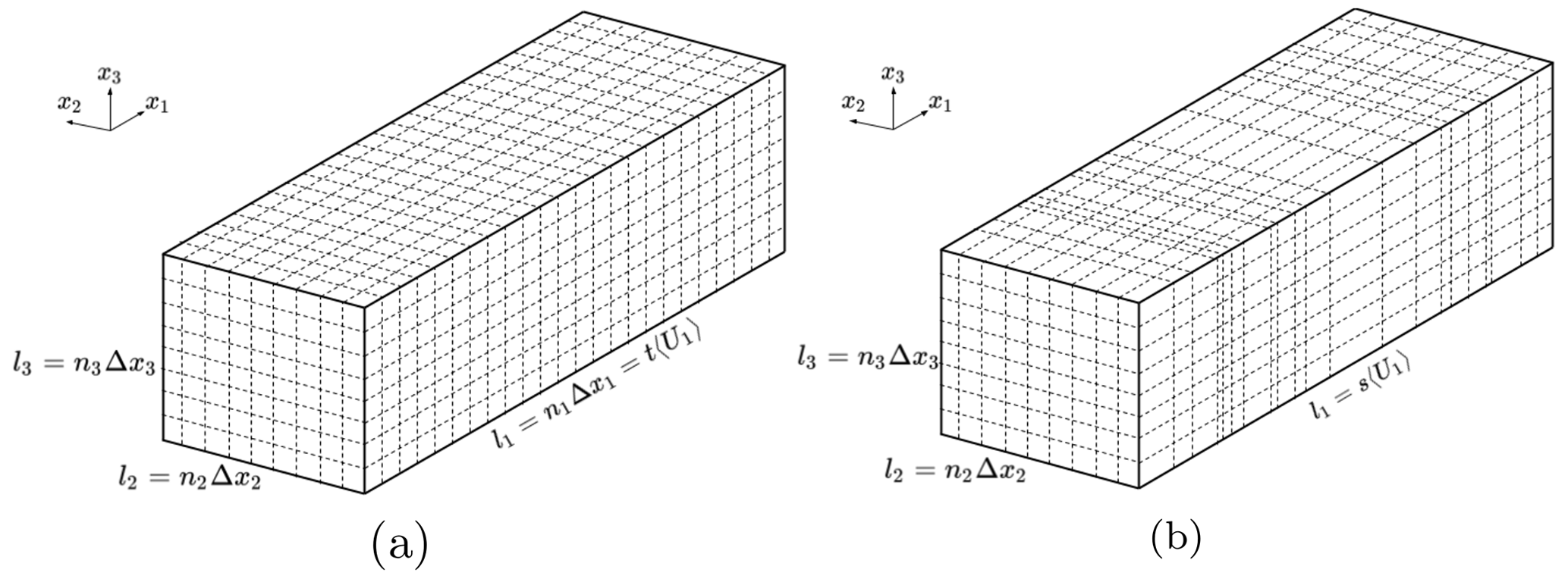
Figure 2 Schematic illustration of turbulence boxes generated by the (a) Mann model with equidistant steps and (b) Time-mapped Mann model after applying the time-mapping process resulting in non-equidistant steps.

The effect of the generated intermittent wind field on loads of a wind turbine is analyzed using a numerical BEM simulation (described in Sect. 4.2). This numerical model requires that the size of the time step Δt of the incoming wind field is equidistant during the simulation. However, as schematically shown in Fig. 2, the time-mapping process described by Eq. (19) generates non-equidistant time steps Δt_n, proportional to τ_α calculated with Eq. (18). Therefore, the wind speed U_i has to be linearly interpolated between the discrete points obtained with the random numbers τ_α to the required discrete points distanced by a fixed time increment Δt_BEM. An example of this interpolation is graphically illustrated in Fig. 3. The dashed vertical red lines correspond to the discrete times from the mapping process separated by Δt_n∝τ_α. The red dots show the process U_i at those discrete times. Similarly, the continuous vertical black lines depict the times equally distanced by Δt=Δt_BEM. Then, the linear interpolation takes place between the red dots to obtain the values of U_i at the times depicted by the black lines. The resulting equally distanced discrete points are shown by the black squares. For clarification purposes, the schematic illustrations shown in Figs. 2 and 3 do not correspond to the same time-mapping process but should just demonstrate the mathematical process.

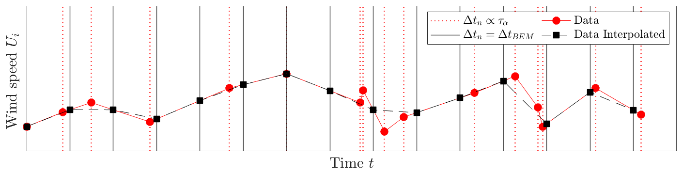
Figure 3 Schematic illustration of the interpolation from non-equally distributed time increments Δt_n∝τ_α to equally distributed time increments Δt_BEM for the BEM simulations.

To generate a Mann box, the HAWC2 Mann turbulence generator tool (DTU Wind Energy, 2018) is used. After that, an in-house MATLAB (MATLAB, 2019) code is used to create the Lévy distribution for τ_α to apply the time mapping and interpolation processes.

4 Results and discussion

In this section, the analysis of the new Time-mapped Mann wind field and exemplary resulting loads from this time mapping will be shown. To clarify the impact of intermittency on the wind fields and loads in this work, all cases will be compared to the original Mann wind field generated with the same parameters to provide a fair comparison between the two models.

4.1 Characteristics of the Time-mapped Mann model

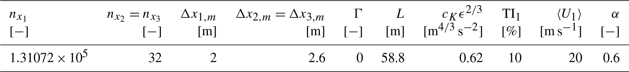
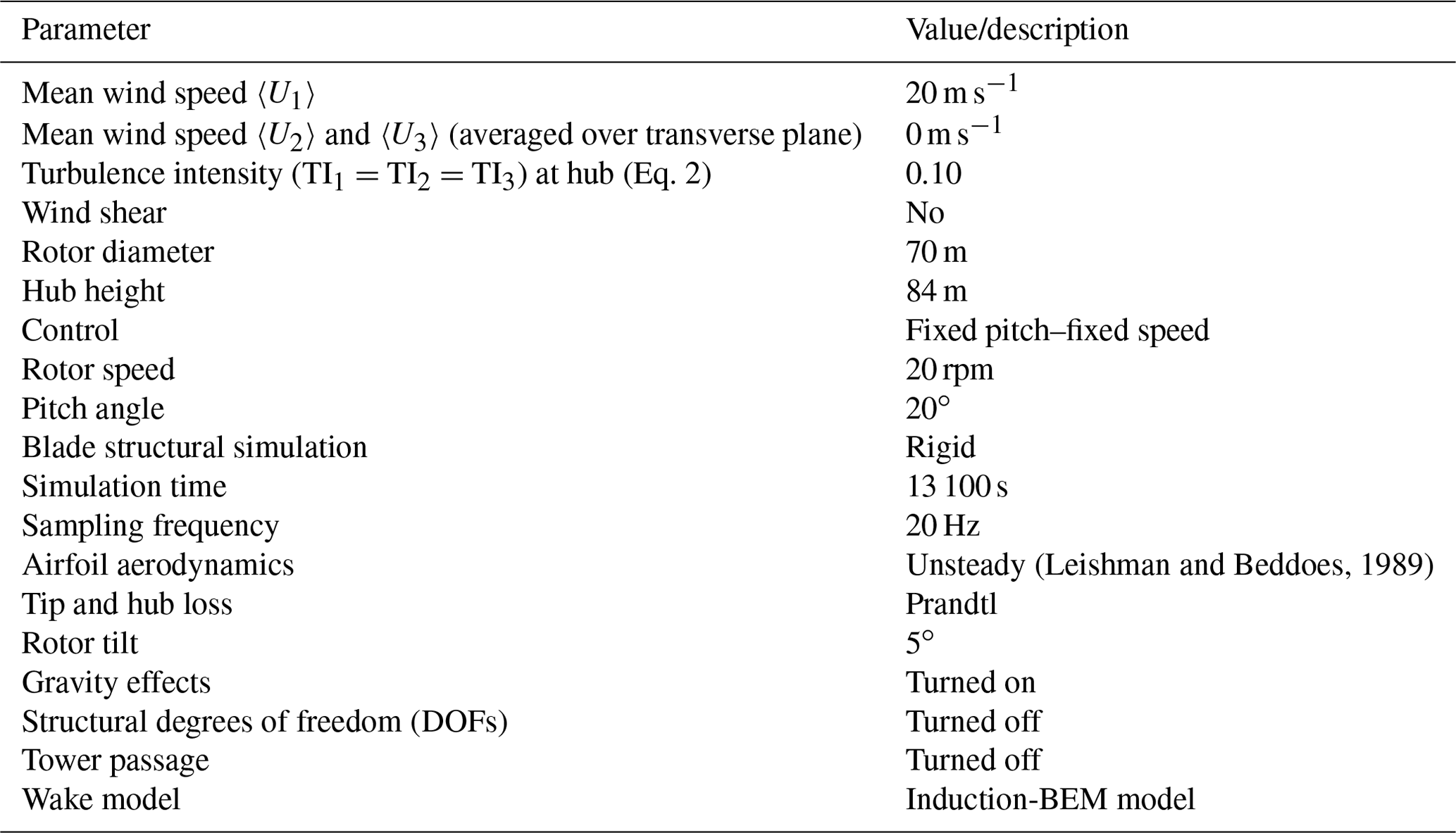
This section provides a thorough comparison of statistical quantities such as the spectral tensors, the coherence, and the velocity increment distribution of both fields, the regular Mann and the new Time-mapped Mann wind field. The dimensions of the grid for the generation of the wind fields are selected according to Table 1, such that they can be used for the BEM simulations in Sect. 4.2. In this case, the defined grid has 32×32 nodes with $\mathrm{\Delta }{x}_{\mathrm{2},m}=\mathrm{\Delta }{x}_{\mathrm{3},m}=\mathrm{2.6}$ m covering an 80.6 m×80.6 m area. The original Mann field is generated using the Mann model at mean wind speed 〈U₁〉=20 m s⁻¹; turbulence intensity in the flow direction, which is the x₁ direction in this case; TI₁=10 %; Γ=0; and $c_K{\mathit{ϵ}}^{\mathrm{2}/\mathrm{3}}=\mathrm{0.62}$ m${}^{\mathrm{4}/\mathrm{3}}$ s⁻² according to the parameters of the Mann model as introduced in the ESDU spectral model. The value of TI₁=10 % was used in this work to keep the same standard deviation value as used for the class B turbine (average class) in the IEC 61400-1 standard (Han, 2007) at 20 m s⁻¹ mean wind speed. Corresponding to Γ=0, we assume homogeneous turbulence and wind shear are not taken into consideration in this work. Also, based on this assumption, the velocity components can be averaged over each slice to calculate the wind field statistics. According to Kelly (2018), the L parameter can be calculated by

$$\begin{array}{}\text{(20)}& L=z{\displaystyle \frac{{\mathrm{TI}}_{\mathrm{1}}}{a}},\end{array}$$

where z is the height of the calculation point (which is the turbine hub height in this work) and a is a shear exponent. Equation (20) is used to calculate the length scale for multi-megawatt wind turbines (Hannesdóttir et al., 2019). However, this equation is also used in the present work for a 1.5 MW wind turbine in order to enable a generalization for larger wind turbines. Even though we assume no shear in this work, the shear exponent value a is only used to calculate the value of L with no effect on the wind velocities. According to the hub height of the studied 1.5 MW turbine with z=84 m and for neutral conditions with a shear exponent of $a=\mathrm{1}/\mathrm{7}$ (Schlichting and Gersten, 2016), Eq. (20) results in L=58.8 m.

Table 1 Mann box and time-mapping parameters for the generated wind fields.

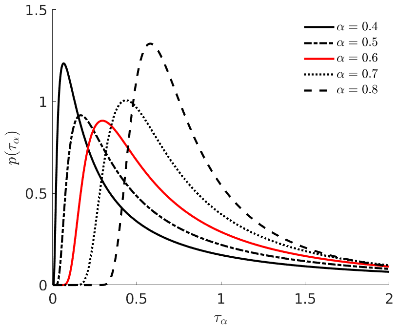
For the Time-mapped Mann wind field, the three components of the velocity fluctuations of each transverse plane (x₂–x₃ in this case) are shifted according to the resulting t(s). When applying the time-mapping process to the wind field, the same stochastic process ($C_{\mathit{\alpha },c,\mathrm{\Delta }{s}_{\mathrm{t}}}{\mathit{\tau }}_{\mathit{\alpha }}\left(s_n\right)$) is applied to each point of the x₂–x₃ plane, and it is not a function of the location of different points in the x₂–x₃ plane. Figure 4 shows the resulting relationship between intrinsic timescale (s) and real-time scale (t) used in the time-mapping process of the original Mann field to the new Time-mapped Mann field according to Eq. (19) for different values of α (in the Lévy distribution). As noticed from this figure, the relationship between s and t is not an exact straight line, which means that the resulting field will be different from the original field as explained in Sect. 3. The values of τ_α in Eq. (19) follow a Lévy's distribution with the corresponding PDFs presented in Fig. 5 at different values of α. In the following analysis and simulations, we will only consider α=0.6, which is highlighted with red lines in Figs. 4 and 5. Additionally, values of c=20 and Δs_t=8 s were considered for the calculation of the scaling factor $C_{\mathit{\alpha },c,\mathrm{\Delta }{s}_{\mathrm{t}}}$ in Eq. (19). These parameters were selected through an iterative process to achieve values of Kurt(v₁), defined in Eq. (11), in a comparable range to the data shown in Fig.1 and to other literature values like Schwarz (2020). The iteration aimed not only to find values of the parameters that match the desired values of Kurt(v₁) but also to keep other statistical values such as the standard deviation and the spectrum of the time series of the wind velocity.

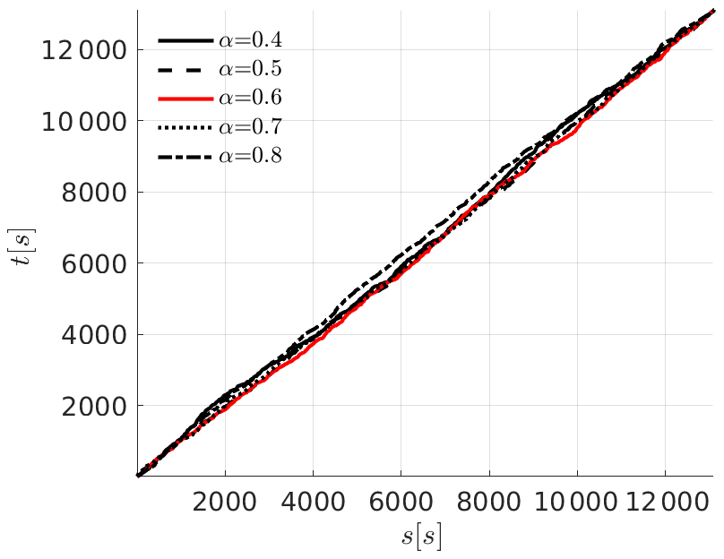
Figure 4 Relationship between the intrinsic timescale (s) and physical timescale (t) (resulting from τ_α in Eq. 19) at different values of α.

Figure 5 Lévy probability distribution of τ_α as in Eq. (17) at different values of α.

The comparison between the Mann and the new Time-mapped Mann wind fields regarding statistical properties is performed in terms of one-point and two-point statistics from Sect. 2.1. Starting with one-point statistics, the values of the mean wind speed in the longitudinal direction U₁ and the corresponding standard deviation $\sqrt{\langle u_{\mathrm{1}}^{\mathrm{2}}\rangle }$ are presented in Table 2. These values are calculated from the time series at the hub point (location of the hub of the turbine in the BEM simulations; see Sect. 4.2). For better comparison, the relative differences (Rel.Diff) calculated as the difference between both results over the result from Mann field (i.e., ($\text{Time-map.}-\text{Mann})/\text{Mann}$) are also presented in the table.

Table 2 Values of the mean wind speed and standard deviation at the hub point in the longitudinal direction (〈U₁〉 and $\sqrt{\langle u_{\mathrm{1}}^{\mathrm{2}}\rangle }$) for the Mann (Mann) and Time-mapped Mann (Time-map.) wind fields.

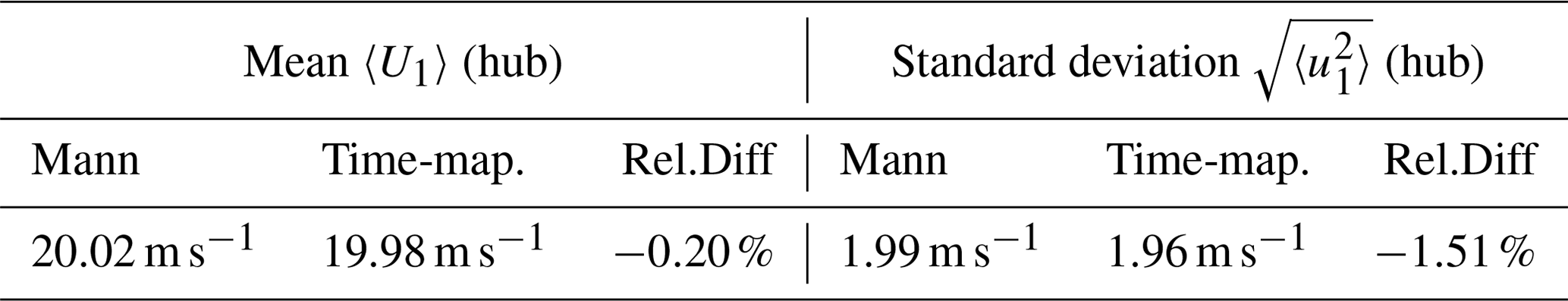
The values of the relative differences for 〈U₁〉 and $\sqrt{\langle u_{\mathrm{1}}^{\mathrm{2}}\rangle }$ are lower than 2 %. This means, in terms of one-point statistics at the hub point, that the two generated wind fields are comparable. The slight differences between the two fields are caused by the interpolation procedure explained in Fig. 3. However, one-point statistics are not enough to show the effects of intermittency.

To show the effect of the time mapping on the spectral properties of the new field, Fig. 6 shows a comparison between the spectra κ₁〈F_i(κ₁)〉_ℐ of three components of the original Mann field and the new Time-mapped Mann field where ${\mathit{\kappa }}_{\mathrm{1}}=\mathrm{2}\mathit{\pi }f/U_{\mathrm{1}}$. In these figures, 〈.〉_ℐ denotes spatial averaging over the plane $\mathcal{I}=\mathit{\left\{}\right(x_{\mathrm{2}},x_{\mathrm{3}}\left)\right|\mathrm{0}\le x_{\mathrm{2}}\le l_{\mathrm{2}},\mathrm{0}\le x_{\mathrm{3}}\le l_{\mathrm{3}}\mathit{\}}$. Figure 6a shows the wavenumber spectrum of the u₁ velocity component in the longitudinal (x₁) direction, while Fig. 6b and c show the same comparison but for the u₂ component in the x₂ direction and the u₃ component in the x₃ direction, respectively. The theoretical spectra of the Mann field from Eq. (14) are plotted in the same figures to show how the spectra should be distributed over the different wavenumbers. Further to that, an uncorrelated, intermittent wind field was also added for the comparison. This uncorrelated wind field is generated by arbitrarily shuffling the grid points of the intermittent Time-mapped Mann field in the transverse directions (x₂ and x₃ directions). Of course, that still means that all points in the x₂–x₃ plane are shifted by the same time step in the temporal direction, but now the spatial correlations in the x₂–x₃ directions are disturbed by mixing. This uncorrelated field is generated to show the difference between a correlated field in the transverse direction (which is the Time-mapped Mann field) and a completely uncorrelated turbulent field in the transverse direction.

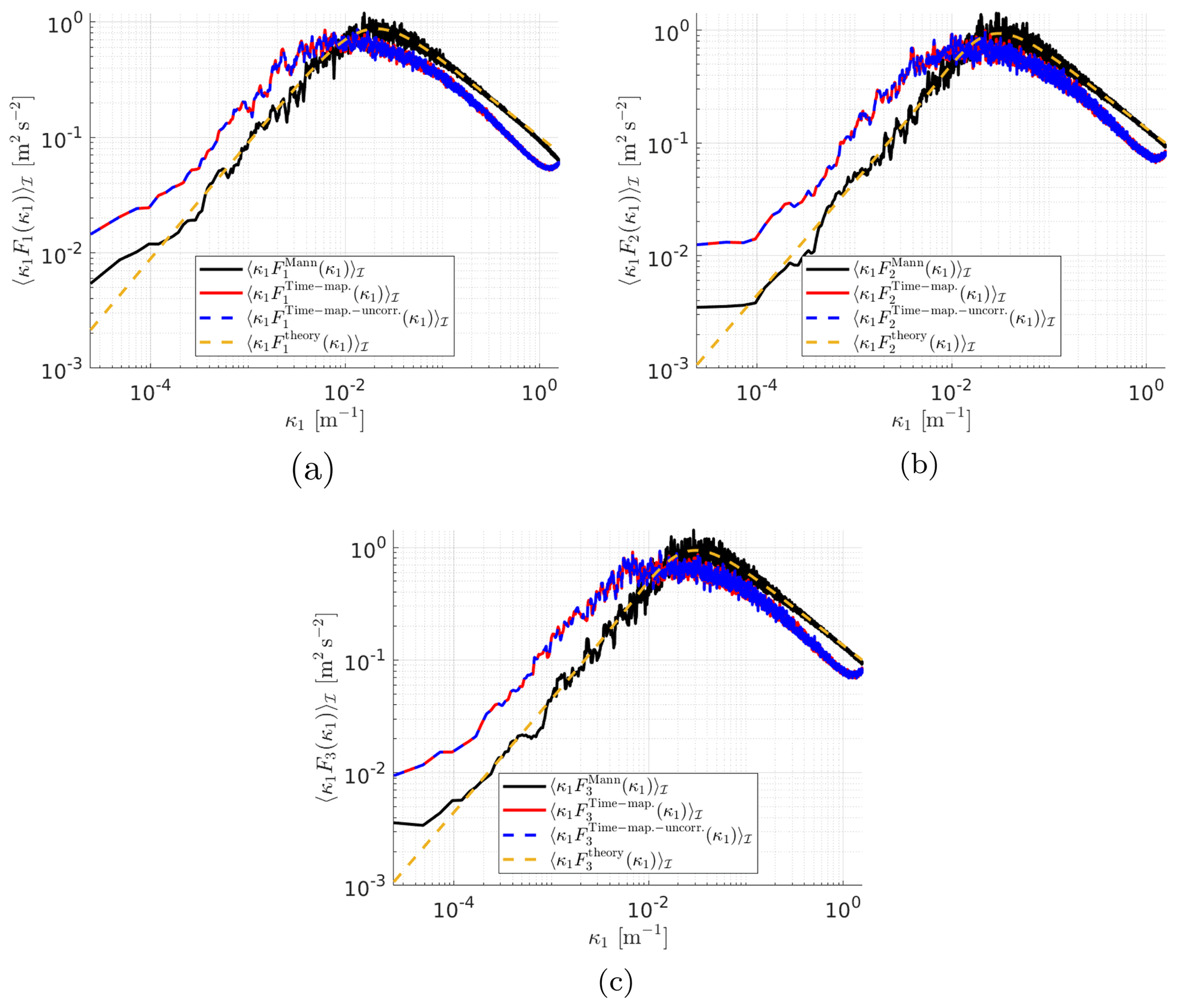
Figure 6 Comparison of averaged spectra in the (a) x₁, (b) x₂, and (c) x₃ directions for the Mann field ($F_i^{\mathrm{Mann}}\left({\mathit{\kappa }}_i\right)$), the Time-mapped Mann field ($F_i^{\text{Time-map.}}\left({\mathit{\kappa }}_i\right)$), an uncorrelated Time-mapped Mann field (e.g., $F_i^{\text{Time-map.-uncorr.}}\left({\mathit{\kappa }}_i\right)$), and the theoretical spectra ($F_i^{\mathrm{theory}}\left({\mathit{\kappa }}_i\right)$) calculated from Eq. (14).

Figure 6 shows the change in spectra due to the application of time mapping on a turbulent Mann field. Discrepancies between the two fields arise from the time-mapping process and the interpolation procedure. The fields analyzed in Fig. 6 are the fields generated without re-scaling as explained in Sect. 2.2 to make sure that the analyzed fields keep their original characteristics before applying any mathematical scaling. It can be noticed from the figures that the peak values of κ₁F₁(κ₁) occur at lower κ₁ values compared to the theoretical and the Mann spectra, and the time-mapped spectra curves are shifted to the lift, i.e., towards lower κ₁ values. Such a shift results from the time-mapping process that slightly changes the characteristics of the resulting field. Also, the time-mapped field has a lower peak value of κ₁F₁(κ₁). It is expected that such a decrease happens due to the interpolation introduced to the Mann model during the time-mapping process.

From turbulence theory, there exist many other models which address more statistical characteristics and are based on a proper superposition of Gaussian statistics (Rosales and Meneveau, 2006). A similar approach has also recently been applied to the Mann model where the small-scale Gaussian statistics of Mann wind fields with varying covariances were superposed to yield small-scale intermittency (Friedrich et al., 2021). However, our intention is to combine well-established models in wind energy which we did by combining the Mann model with the time-mapping procedure from the CTRW model. As a consequence, our model shows spatial correlations in the x₂–x₃ plane similar to the Mann model and allows us to investigate the influence of temporal intermittency. For the uncorrelated intermittent field, a comparable agreement as in the correlated case between this field and the Time-mapped Mann field in the longitudinal direction x₁ can be seen since the arbitrary shuffling was only applied in the transverse directions.

The new model allows a detailed comparison between Gaussian Mann and non-Gaussian Time-mapped Mann fields. This comparison is shown in detail in this work. For further investigation of these deviations between Mann and Time-mapped Mann fields, Fig. A1 shows the same spectra as shown in Fig. 6 but with an equal number of grid points in all directions (in this case, $n_{x_{\mathrm{1}}}=n_{x_{\mathrm{2}}}=n_{x_{\mathrm{3}}}=\mathrm{512}$). This case is referred to as the “cubic case”. The spectra of these fields in Fig. A1 show that for a lower number of grid points in the x₁ direction, the differences in spectra between Mann and the Time-mapped Mann field are lower.

As indicated in Sect. 2.1, the velocity spectrum is not sufficient to show intermittency. Therefore, increment statistics should be used in this case to show the effects of intermittency. The coherence of velocity components (Eq. 6) of the two wind fields in the three spatial directions is plotted versus κ₁Δx₂ in Fig. 7 with Δx₂=2.6 m. In this figure, the difference in the coherence of the two fields, as we move in the x₂ direction, is obvious due to the time mapping in the longitudinal direction. The Mann model is based on the von Kármán energy spectrum, which is reflected by the coherence of the Mann-modeled wind field. On the other hand, a comparison between the coherence of the two wind fields versus κ₂Δx₃ for the cubic case is shown in Fig. A2 in the Appendix. In the latter case, the differences in coherence between the two fields are small. This is due to the unchanged x₂–x₃ planes during the time-mapping process. This shows that the coherence with respect to the longitudinal direction is highly influenced by the time mapping, whereas it is not with respect to the transverse direction. That shows that the time mapping goes at the cost of the spatial correlations in the x₁ direction, which is expected since the x₁ axis is stretched and compressed, which is also reflected by the spectrum in the x₁ direction in Fig. 6a. By comparing Figs. 7 and A2, it can be noticed that the plots in Fig. A2 look smoother. This is also due to the difference in the number of grid points in the x₁ direction between the two cases.

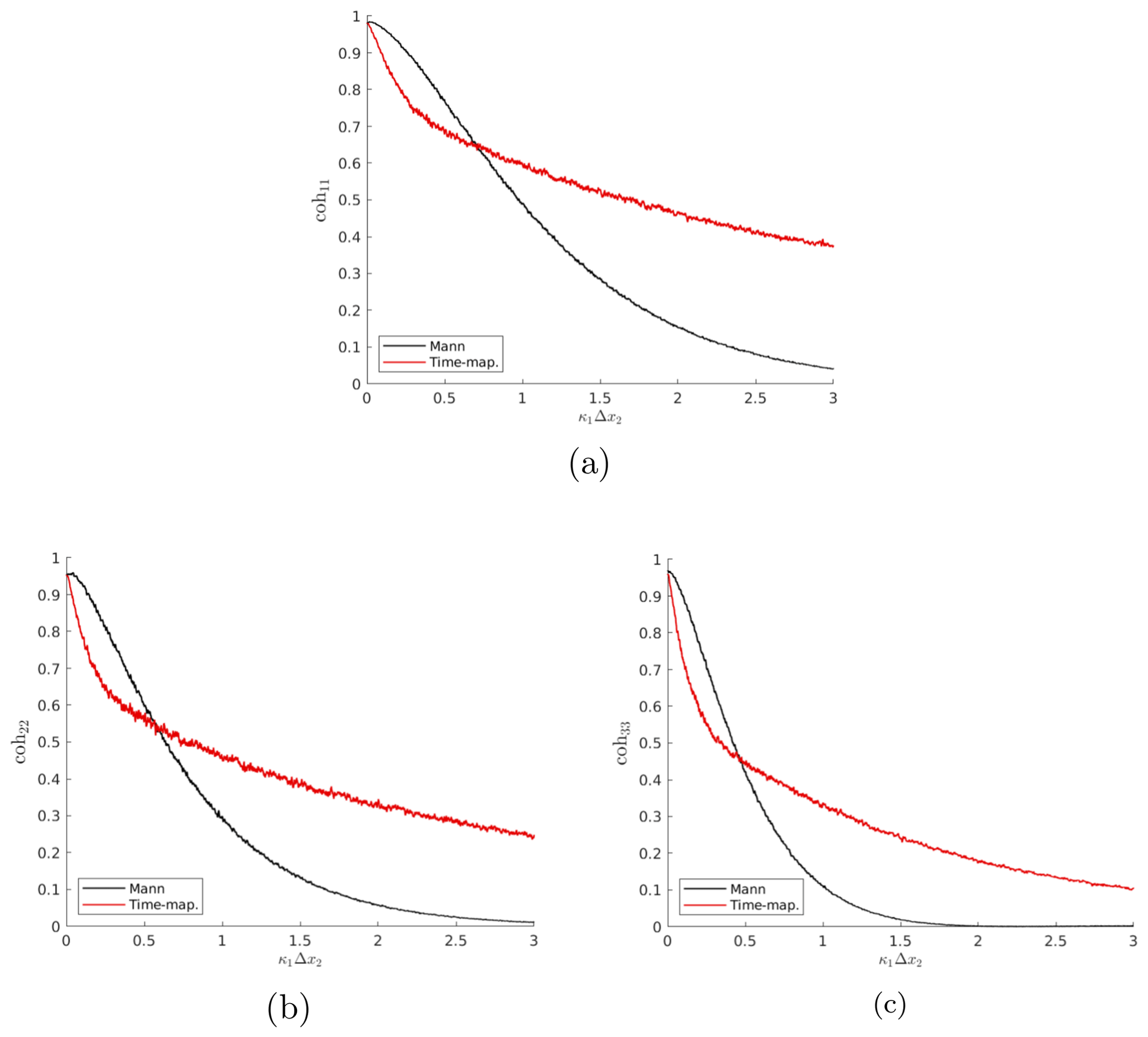
Figure 7 Comparison of the coherence of velocity components in the (a) x₁, (b) x₂, and (c) x₃ directions for both Mann and Time-mapped Mann fields over wavenumber κ₁Δx₂ with Δx₂=2.6 m and Δx₃=0. Dark lines represent smoothed coherence values of the light lines using a moving average method.

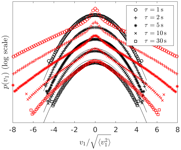
Figure 8 Spatially averaged PDF over transverse planes of velocity increments of the Mann wind field (black) and the Time-mapped Mann wind field (red) at different temporal increments τ. The black thin lines are Gaussian distributions as a reference. In principle, the curves would all lie on top of each other, but here the curves are shifted vertically for a better visualization.

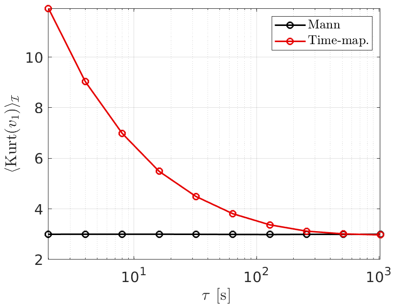
Figure 9 Kurtosis of Mann (black) and Time-mapped Mann (red) fields (Eq. 11) at different temporal increments τ. For a Gaussian distribution, the kurtosis is 3.

Following on from the two-point statistics analysis, the velocity increments v₁ defined in Eq. (10) and the degree of intermittency of the wind fields are analyzed. Figure 8 shows the comparison between the PDFs of the velocity increment of both the Mann and the new Time-mapped Mann wind fields. It is obvious in this figure how extreme events in the case of the time-mapped wind field (the red markers) have a higher probability than the corresponding events in the case of the Gaussian Mann field (the black markers). Also, it can be noticed that the intermittency increases with the decrease in τ. Note that this τ refers to the temporal increment in Eq. (10) and not to the τ_α introduced in the context of the Lévy distribution. Another important measure of the increment statistics is the kurtosis calculated from Eq. (11). In the case of the kurtosis of the wind fields, the angular brackets denote averaging over time, and kurtosis, in this case, is only a function of τ. Figure 9 shows a comparison between the kurtosis of the velocity increment from the Mann field and the Time-mapped Mann fields at different τ values. As explained earlier, higher values of τ show a Gaussian distribution with kurtosis of 3, and lower values of τ show more deviation from the Gaussian PDF of the Mann field.

4.2 Analysis of the resulting wind turbine loads

After analyzing the effect of the time mapping on the different statistics of the wind fields in the previous section, here the effect on exemplary turbine loads is studied. The main point of this section is to see whether the intermittency from the wind field is carried to the turbine structure. If the turbine loads are proven to reflect intermittency, this might have a significant effect on the dynamic loads acting on the wind turbine. For example, the damage equivalent loads (DEL) calculated from fatigue analysis might be affected due to intermittency because the probability for extreme values in the load increments is larger than for a Gaussian distribution.

In this work, BEM simulations of the NREL WindPACT 1.5 MW (Malcolm and Hansen, 2006) virtual wind turbine are performed using the aeroelastic simulator NREL FAST (v8.16) (Jonkman and Jonkman, 2016). The main characteristics of the turbine and input parameters for the simulations are summarized in Table 3. The wind fields used in these simulations are the same Mann and Time-mapped Mann fields analyzed and compared in Sect. 4.1.

Leishman and Beddoes, 1989

Table 3 Main parameters of the turbine and numerical simulations. A description of the listed set-ups for the BEM simulation can be found in Jonkman et al. (2016) and Jonkman and Jonkman (2016).

Four different load sensors were selected for analyzing the effect of the intermittent wind: the bending moment at the root of the blade in the flapwise direction (RootFlap), the rotor torque (Torque), the rotor thrust (Thrust), and the bending moment at the base of the tower in the fore–aft direction (TwrForeAft). According to Schwarz (2020), these four sensors are expected to be highly sensitive and mainly dominated by aerodynamic forces in the direction of the flow and not by other sources of load such as gravitational forces.

Firstly, the mean values and standard deviations calculated over the length of the simulation are presented in Table 4. Here, the results for the four load sensors of both the Time-mapped Mann (Time-map.) and the Mann (Mann) wind field are shown. Moreover, the relative differences (Rel.Diff) were also calculated (i.e., ($\text{Time-map.}-\text{Mann})/\text{Mann}$).

Table 4 Mean values and standard deviations of time series from BEM simulations for the Mann (Mann) and the Time-mapped Mann (Time-map.) wind fields. The relative differences (Rel.Diff) between the two cases are calculated for better interpretation.

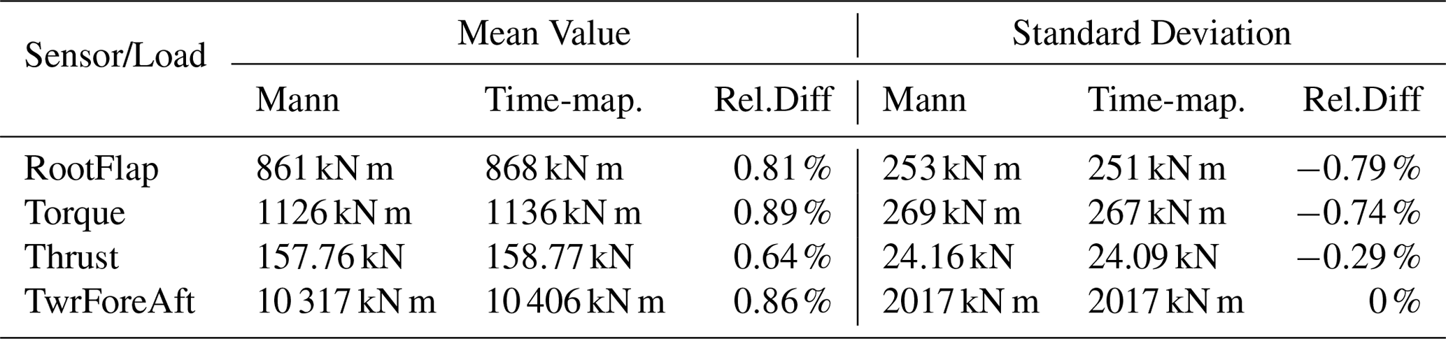
In Table 4, the relative differences of the mean values and standard deviations of the analyzed sensors are less than ±1 % between the Mann and the Time-mapped Mann wind field. It can be seen that this difference is in the same order as the differences in the mean wind speed 〈U₁〉 and standard deviation $\sqrt{\langle u_{\mathrm{1}}^{\mathrm{2}}\rangle }$ at the hub point presented in Table 2. To investigate whether the intermittency in the wind field carries over to the turbine loads, the incremental statistics of the loads are evaluated. The load increments M_τ are defined similarly to velocity increments in Eq. (10):

$$\begin{array}{}\text{(21)}& M_{\mathit{\tau }}(t,\mathit{\tau })=M(t+\mathit{\tau })-M\left(t\right),\end{array}$$

where M is the time series of the load sensor and τ corresponds to the time lag. Figure 10 shows the PDFs of M_τ for the four selected load sensors, for τ=3 s (top) up to τ=30 s (bottom) for the blade root flapwise bending moment and τ= 1 s (top) up to τ=30 s for the rotor thrust, rotor torque, and tower fore–aft bending moment. For a direct comparison to the PDFs of the velocity increments v₁, the values of τ are selected analogously to Fig. 8. Similar to Figs. 1 and 8, all the individual PDFs are normalized to standard deviation $\sqrt{\langle M_{\mathit{\tau }}^{\mathrm{2}}\rangle }=\mathrm{1}$. Here, the angular brackets denote moving averages over the time series.

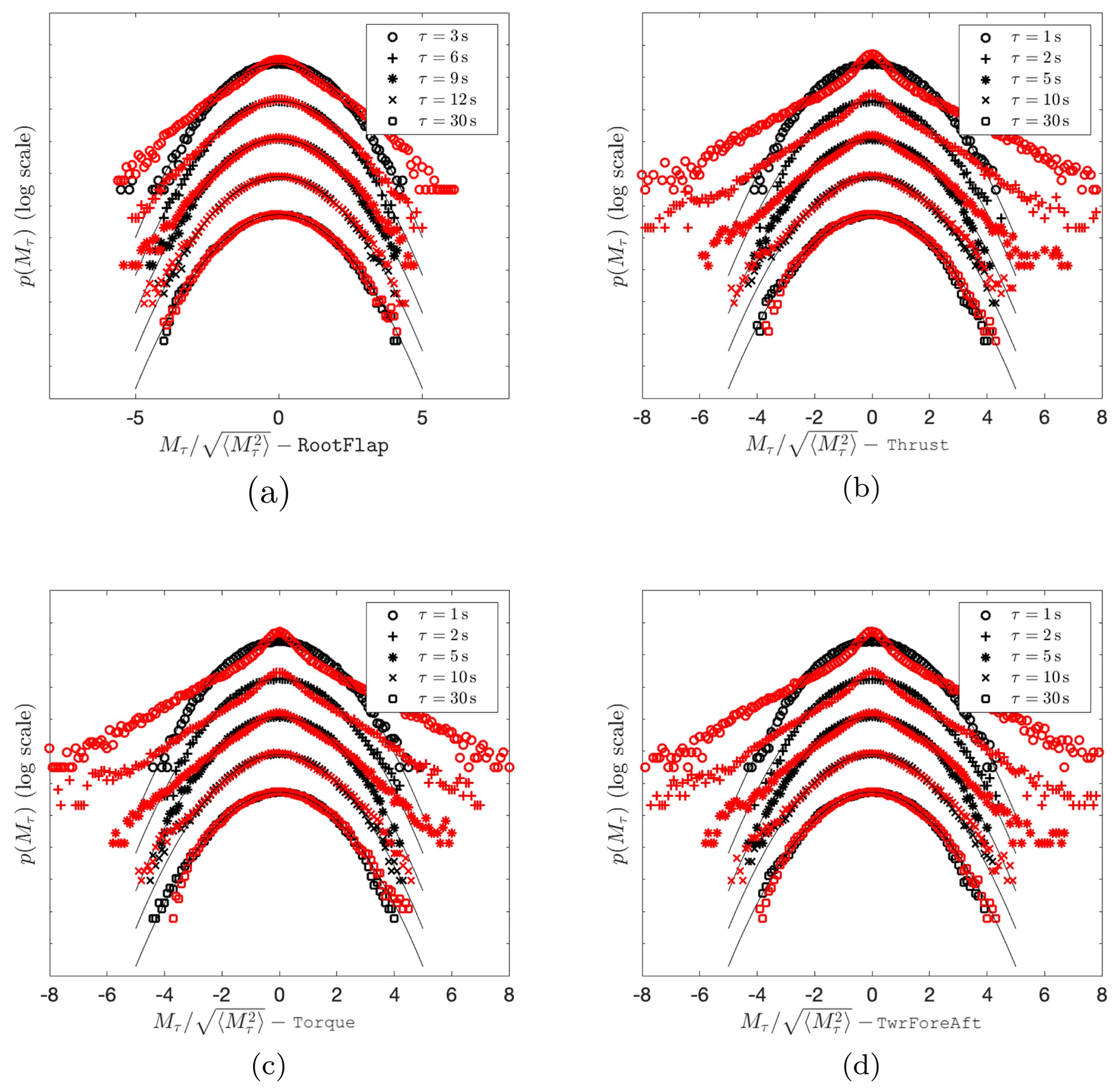
Figure 10 PDFs of load increments M_τ for the (a) blade root flapwise bending moment (RootFlap), (b) rotor thrust (Thrust), (c) rotor torque (Torque), and (d) tower fore–aft bending moment (TwrForeAft) of the 1.5 MW turbine with Mann and Time-mapped Mann inflow wind fields at different temporal increments τ. The red markers correspond to the Time-mapped Mann field cases, while the black markers present the results for the Mann field cases. The black thin lines are Gaussian distributions as reference. The curves are shifted vertically for visualization.

The resulting load increments M_τ follow the characteristics of the wind velocity increments shown in Fig. 8. The PDFs of the Mann load increments are very well described by the Gaussian distribution. On the contrary, the PDFs of the load increments resulting from the Time-mapped Mann field deviate significantly from the Gaussian distribution for a range of scales. The observed heavy tails shown by the time-mapped PDFs reflect, as mentioned earlier, a higher probability of extreme load fluctuations than the probability of a Gaussian distribution.

Figure 10a shows a special case for the RootFlap load. The shown τ values differ from the other loads to make the intermittency visible in this case. The RootFlap moment is dominated by the 1P frequency while the other loads are dominated by the 3P frequency. Consequently, showing the same τ values in Fig. 10a as for the other loads would not reveal the intermittency in our special case. The energy spectra of the RootFlap and Thrust are shown in Appendix B for a deeper understanding of the different frequencies of the loads.

Also, it turns out that the frequencies of the energy spectra carry over to the frequencies in the kurtosis, as shown in Fig. 11 for the thrust. A more detailed description of the evolution of the intermittency of M_τ with τ is presented in Fig. 11. Here, the results of Kurt(M_τ) from Eq. (11) are calculated exemplarily for the Thrust signal. It is visible that the values of the kurtosis for the load case with the Time-mapped Mann wind field are higher than 3 (the value of 3 indicates a Gaussian distribution) for all the values of τ up to around 20 s. This proves the intermittent characteristics of the loading. In contrast, the corresponding values for the Mann case fluctuate around 3 for all the considered timescales, agreeing with the Gaussian statistics. Additionally, for timescales below 1 s, a decreasing intermittent behavior of the load is visible in the time-mapped case when decreasing τ. The kurtosis of the thrust in Fig. 11 is overall lower than that of the corresponding wind field as shown in Fig. 8. This has been also shown by Mücke et al. (2011), who have used an atmospheric wind measurement as input to calculate the torque.

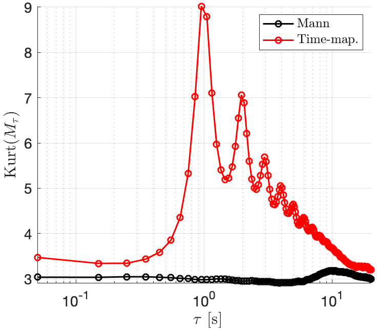
Figure 11 Kurtosis of the PDF of M_τ calculated for the Thrust according to Eq. (11) at different temporal increments τ. The red markers correspond to the Time-mapped Mann field, while the black markers present the results for the Mann field. A value of 3 corresponds to a Gaussian distribution.

Further investigations should be done to explain the potential sources of the observable bumps in the kurtosis of the Time-mapped Mann case. A strong dependence of the peaks on the rotational frequency of the rotor has been recognized by the authors. However, this first turbine study aimed at investigating whether the intermittency which was introduced to the wind field by deriving the Time-mapped Mann field carries over to turbine loads in general. This has clearly been shown here.

5 Conclusions

In this work, a new synthetic wind field model has been introduced which combines spatial correlations from the well-known Mann model and the effect of intermittency. During the derivation, the time-mapping procedure from the so-called CTRW model has been applied to a Mann wind field to generate intermittency. This new model is called the Time-mapped Mann model. The CTRW model relies on stochastic differential equations for the velocity and assumes exponentially decaying velocity correlations. On the other hand, the Mann model is based on a proper modeling of the spectrum according to atmospheric conditions which are also recommended by the standard IEC 61400-1. With our procedure, we obtain a model which aims at keeping the spatial correlations in the transverse directions from the Mann model, thus following the IEC 61400-1 standard in this respect, and on the other hand adding intermittency, which has also been reported as a feature inherent in the wind field (Mücke et al., 2011).

The analysis of the velocity spectra, as well as the PDF and kurtosis of velocity increments, showed that this method managed to generate an intermittent wind field in the longitudinal direction. On the other hand, this method keeps the spatial correlation almost exactly as in the Mann field in the other two directions. This is due to the way the time mapping is applied where the velocity field “slices” (x₂–x₃ planes) of the Mann field are shifted by random time shifts. Small differences in the compared statistics in transverse directions are due to the interpolation between the generated time-shifted slices and the new, uniformly separated velocity field slices.

Furthermore, the first analysis and comparison of loads with respect to intermittency between Mann and time-mapped wind fields on a 1.5 MW wind turbine was done. The analysis of the loads showed that the intermittency is transported from the wind field to the structure of the wind turbine. However, these loads are different in their response to the wind field intermittency. The increment statistics showed that in the analyzed case, the rotor thrust, rotor torque, and tower fore–aft bending moment are strongly affected by the intermittency in the wind field, whereas the blade root bending moment shows less intermittency. The resulting non-Gaussian load increment distributions suggest that simulating wind turbines under Gaussian wind fields such as Mann wind fields could potentially lead to an underestimation of the probability of extreme loads.

An important future extension of the Time-mapped Mann model would be an incorporation of shear in the Time-mapped Mann model. The original Mann model has the option of imposing eddy stretching to account for shear. However, it may not be a straightforward process to add this eddy stretching to the Time-mapped Mann field. The first question is whether the eddy stretching should be added before or after the time mapping, whereas the option to add it before the time-mapping process may seem more reasonable. In the future, the Time-mapped Mann model will be extended to incorporate the wind shear. Further, it has to be investigated if the areas with larger mean velocity should have a different time mapping.

Also, in future research based on this work, the different turbine loads and their response to turbulent inflow with intermittency could be investigated in more detail. This investigation should also involve different sizes of wind turbines that cover a larger area of the wind fields, as well as variable speed, and variable pitch wind turbines at a variety of wind conditions. For example, such wind conditions could be measured from wind sites to have better anticipation of the turbine loads in the presence of intermittency. Another possible future work would be to compare the impact of intermittency on different wind turbine loads at different wind speeds to investigate whether there are effects of wind speeds on the loads' intermittency. Additionally, fatigue load could be a subject of further investigation, which requires further discussion since the rain flow cycle counting method may not detect intermittency properly as discussed by Mücke et al. (2011).

Appendix A: Analysis of a cubic field

For a further investigation of the effect of the time mapping of wind fields on the spectra, a Mann box with $n_{x_{\mathrm{1}}}=n_{x_{\mathrm{2}}}=n_{x_{\mathrm{3}}}=\mathrm{512}$ and $\mathrm{\Delta }{x}_{\mathrm{1},m}=\mathrm{\Delta }{x}_{\mathrm{2},m}=\mathrm{\Delta }{x}_{\mathrm{3},m}=\mathrm{1}$ m is studied in this Appendix. The same comparison of spectra as described in Sect. 4.1 is studied here for this cubic field. As introduced in the previous sections, there are three different parameters used to generate the box: the overall box size, the grid cell size, and the number of cells. Since it is not possible to change the value of one of these parameters alone without changing at least one of the other two parameters to generate a grid with comparable results, a new grid with cubic cells was generated to have independence of the direction since all directions have the same grid points and cell sizes.

In Fig. A1a, b, and c it can be seen that the spectra show generally good agreement between the Mann and the Time-mapped Mann field. The spectra in the longitudinal direction x₁ in Fig. A1a show a discrepancy due to the time-mapping procedure which is applied to this direction. Further, all plots show increasing discrepancies for larger wavenumbers which should result from the interpolation procedure. Note that in Fig. 6b and c where the resolution in the x₂ and x₃ direction was much coarser, the deviations already start at smaller wavenumbers. The comparison of coherence of the same two fields in Fig. A2 shows good agreement between the two fields in the x₂ and x₃ directions. The small deviations result from the interpolation routine.

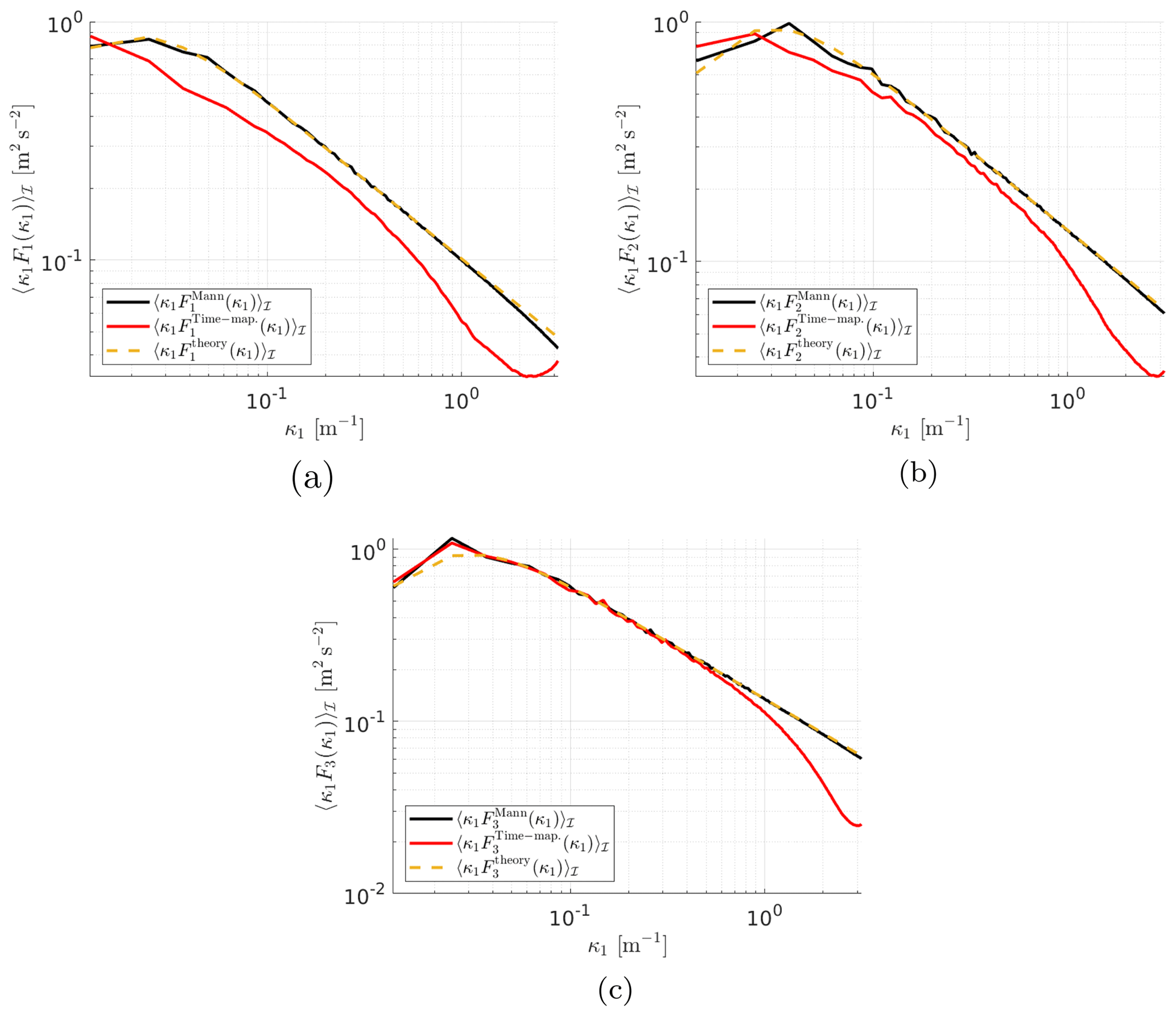
Figure A1 Comparison of averaged spectra in the (a) x₁, (b) x₂, and (c) x₃ directions, respectively, for the Mann field, the Time-mapped Mann field, and the theoretical results calculated from Eq. (14).

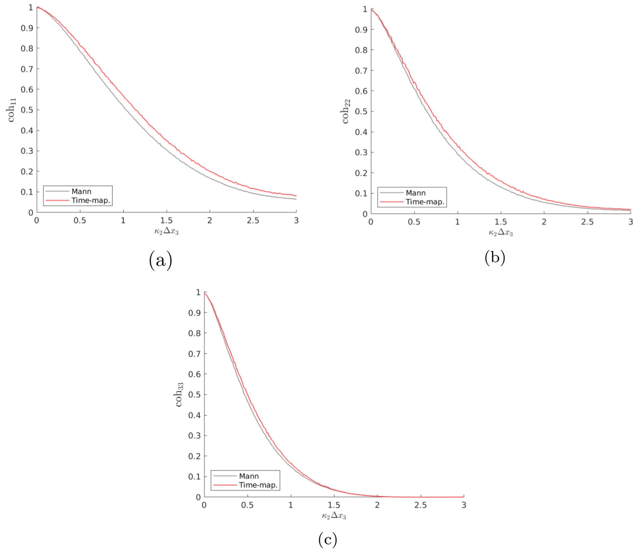
Figure A2 Comparison of the coherence of velocity components in the (a) x₁, (b) x₂, and (c) x₃ directions for the Mann field and the Time-mapped Mann field over wavenumber κ₂Δx₃ with Δx₃ = 2.6m and Δx₁ = 0.

Appendix B: Analysis of the energy spectra of different loads

To investigate the phenomenon shown in Fig. 10a, in which the RootFlap shows intermittency at other τ values, Fig. B1 shows a comparison between the energy spectra of two different loads, namely the blade root flapwise bending moment RootFlap and the rotor thrust Thrust. It can be seen from this figure that the energy spectrum of the Thrust shows peaks at the 3P frequencies and higher, whereas the blade root flapwise bending moment RootFlap shows peaks at the 1P frequency and higher.

This indicates that the fluctuations of the loads happen at different frequencies, which entails applying different τ values in the PDF to be able to see the intermittency as shown in Fig. 10.

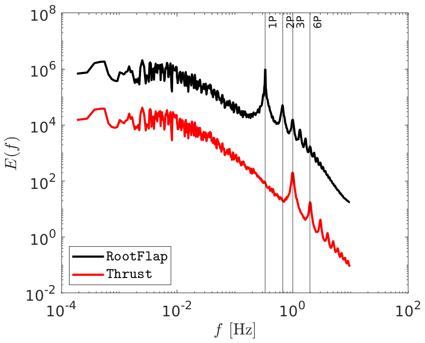
Figure B1 A comparison between the energy spectra of the blade root flapwise bending moment RootFlap and rotor thrust Thrust of the simulated wind turbine under a turbulent wind field generated by the Time-mapped Mann model.