the Creative Commons Attribution 4.0 License.
the Creative Commons Attribution 4.0 License.
 | 17 Jul 2023
Impact of wind profiles on ground-generation airborne wind energy system performance
Martin Dörenkämper
Jochem De Schutter
Curran Crawford
This study investigates the performance of pumping-mode ground-generation airborne wind energy systems (AWESs) by determining cyclical, feasible, power-optimal flight trajectories based on realistic vertical wind velocity profiles. These 10 min profiles, derived from mesoscale weather simulations at an offshore and an onshore site in Europe, are incorporated into an optimal control model that maximizes average cycle power by optimizing the trajectory. To reduce the computational cost, representative wind conditions are determined based on k-means clustering. The results describe the influence of wind speed magnitude and profile shape on the power, tether tension, tether reeling speed, and kite trajectory during a pumping cycle. The effect of mesoscale-simulated wind profiles on power curves is illustrated by comparing them to logarithmic wind profiles. Offshore, the results are in good agreement, while onshore power curves differ due to more frequent non-monotonic wind conditions. Results are references against a simplified quasi-steady-state model and wind turbine model. This study investigates how power curves based on mesoscale-simulated wind profiles are affected by the choice of reference height. Our data show that optimal operating heights are generally below 400 m with most AWESs operating at around 200 m.
- Article
(8793 KB) - Full-text XML
- BibTeX
- EndNote


Airborne wind energy systems (AWESs) aspire to harvest stronger and less turbulent winds at mid-altitude, here defined as heights between 100 and 1000 m, presumably beyond what is achievable with conventional wind turbines (WTs). The prospects of higher energy yield combined with reduced capital cost motivate the development of this new class of renewable energy technology (Lunney et al., 2017; Fagiano and Milanese, 2012). Unlike conventional WTs, which in recent decades have converged to a single concept with three blades and a conical tower, several different AWES concepts and designs are being investigated by numerous companies and research institutes (Cherubini et al., 2015; Vermillion et al., 2021; Fagiano et al., 2022). These kite-inspired systems consist of three main components: one or more tethered aircraft or kites, one or more ground stations, and one or more tethers to connect the flying components to the ground. This study focuses on the two-phase cyclic, ground-generation concept, also referred to as pumping mode (Luchsinger, 2013). During the reel-out or production phase, the kite pulls a tether from a drum on the ground, which is connected to a generator, thereby producing electricity. This is followed by the reel-in phase during which the kite returns to its initial position and reduces its aerodynamic forces in order to de-power. There are several ways to reduce the aerodynamic forces on a kite, such as adjusting its angle of attack or flying it out of the wind window. Various other concepts such as fly-gen, aerostat, and rotary lift are not considered in this study (Cherubini et al., 2015). Since this technology is still in a relatively early stage of development, validation and comparison of power production estimates is difficult. Several studies (van der Vlugt et al., 2013; Schelbergen et al., 2020; Vander Lind, 2013; Ranneberg et al., 2018) compared computed power curves with experimental performance data. At present, there is no standardized power curve definition or reference design that would allow for comparison between different concepts and conventional wind turbines. However, the goal of Eijkelhof and Schmehl (2022) and Eijkelhof et al. (2020) was to create a reference design for a multi-megawatt AWES. It is not the goal of this study to determine a general power curve but rather to investigate the power variation in a specific design derived from realistic wind profiles.
Recent consensus among the scientific community defined a power curve as the maximum average cycle power, which is the combination of consecutive reel-out and reel-in phases, as a function of wind speed at pattern height, which is the time-averaged height during the reel-out power-producing phase (Airborne Wind Europe, 2021). Together with the site-specific wind resource, wind park planners and manufacturers can use power curves to estimate annual energy production (AEP), which can be combined with a cost model to determine the levelized cost of electricity (LCOE) and financial viability (Malz et al., 2020a). Unlike conventional WTs, where the wind speed probability distribution at hub height is used to determine AEP, AWES continuously change their operating height, making it difficult to determine AEP with this approach. AWES performance highly depends on the shape and magnitude of the wind speed profile over the operating height range. Using simple wind profile approximations, such as logarithmic or exponential wind speed profiles, can provide an estimate of long-term average conditions. However, these approximations cannot account for the wide range of profile shapes that occur over short periods of time or changes that occur on a daily or seasonal basis (Emeis, 2013). This can reduce the accuracy of the predicted power output. However, such wind speed profiles can be employed to estimate average performance and are the standard in most AWES power estimation studies.
In their study, van der Vlugt et al. (2013) described TU Delft's 20 kW inflatable wing technology demonstrator and compared a statistically derived power curve to results from a theoretical performance model. The wind and power models used in this study were taken from Fechner and Schmehl (2013). The wind model is based on a standard exponential wind speed profile approximation, while the power model uses a multi-phase quantitative susceptibility mapping (QSM). A follow-up study (van der Vlugt et al., 2019) added more detail to specific cycle trajectories. Heilmann and Houle (2013) used exponential wind speed profiles and a standard Rayleigh distribution to estimate performance and cost. Their power curve is modeled based on a QSM by Luchsinger (2013) using the averaged flight path height of the kite as the wind speed reference height. An LCOE between EUR 40 and 110 per megawatt hour was estimated for different annual average wind speeds. Faggiani and Schmehl (2018) used a similar pumping-mode QSM to estimate power output based on wind speed at the operating height of the kite. They developed a cost model to estimate the achievable LCOE of an entire kite wind farm. Their analyses showed that the cost of energy decreases and the quality of the electrical power increases with increasing number of kites. Ranneberg et al. (2018) studied the performance of a soft-kite pumping-mode AWES by determining its power curves at various reference heights for different logarithmic wind profiles. The study found that the yield variation for these logarithmic wind profiles was quite small. Additionally, the yield for a specific site was estimated using detailed wind speed profiles from COSMO-DE, and the results were found to be consistent with more detailed simulations of the EnerKíte EK30 prototype (EnerKíte GmbH, 2022). Leuthold et al. (2018) investigated power-optimal trajectories of a ground-generation multikite configuration for a range of logarithmic wind speed profiles. Three distinct operational regions were identified: Region I where power is used to maintain altitude, Region II where power harvesting increases up to the designed wind speed, and Region III where power extraction is intentionally limited due to the physical constraints of the system. Licitra et al. (2019) estimated the performance and power curve of a fixed-kite ground-generation AWES by generating power-optimal trajectories using a power law approximation of the wind speed profile. The results were validated against data from Ampyx Power AP2 (Licitra, 2018; Malz et al., 2019; Ampyx Power BV, 2020). Eijkelhof and Schmehl (2022) found that mass had a detrimental effect on power-optimal trajectories for a large-scale single-kite fixed-wing AWES. To determine power curves, the authors used normalized average offshore wind speed profiles from the Ijmuiden measurement tower. Sommerfeld et al. (2022) used the same methodology and wind data as in this study to examine the effects of size scaling and improvements in aerodynamic efficiency on a single-kite fixed-wing reference system. The authors found that it is likely better to deploy multiple smaller-scale devices rather than a single large-scale system because of negative mass-scaling effects. De Schutter et al. (2019) analyzed the performance of utility-scale, stacked multikite systems using logarithmic wind speed profiles as boundary conditions for a nonlinear optimization problem. The authors used the same optimization framework as in the present investigation. They found that this multikite strategy could make power generation largely independent of wing size. Malz et al. (2020b) efficiently estimated the performance of a single-kite drag-mode AWES for large wind data sets by combining an optimal control performance model with smart initialization and machine learning. Wind speed profiles from the MERRA-2 reanalysis model (Gelaro et al., 2017) were clustered into characteristic profile shapes and interpolated using Lagrangian polynomials (Sect. 4.4). The authors showed that ordering the wind parameters by the wind speed at the average operational height (300 m) significantly reduced the computation time. Aull et al. (2020) explored the design and sizing of fly-gen rigid-kite systems based on a steady-state model with simple aerodynamic and mass-scaling approximations. At each scale, the relationships between size, efficiency, power output, and cost were determined. The wind resource was described by an exponential wind shear model with a Weibull distribution. The main conclusion was that physics and economics favor a larger number of small units. Bechtle et al. (2019) used ERA5 reanalysis data to assess wind resources at high altitudes throughout Europe. They described the available wind energy without considering a specific conversion mechanism and included a description of wind speed and probability at various heights. The effect of variable height harvesting was demonstrated for a location in the English Channel. Schelbergen et al. (2020) proposed a clustering procedure to obtain wind statistics from the Dutch Offshore Wind Atlas (DOWA) data set. Principal component analysis and k-means clustering were used to determine representative wind speed profile shapes. To estimate the AEP of a small-scale pumping AWES located at Cabauw in the center of the Netherlands, several power curves were derived for each wind speed profile shape using a flexible-kite, pumping-mode QSM developed by van der Vlugt et al. (2019). Faggiani and Schmehl (2018) studied the economic impact of various design aspects of wind parks, including the spatial stacking of systems, the number of units, the size of kites, and phase-shifted operation. The performance of the system was estimated using a QSM developed by Schmehl et al. (2013) and van der Vlugt et al. (2019), assuming a range of wind speeds at the operating height of the kite. The AEP LCOE could be assessed by combining a detailed cost model with an assumed Weibull probability distribution. The study found that increasing the number of kites had several scale effects, such as decreasing the cost of energy and increasing the quality of electrical power. Wind speed profiles are governed by weather phenomena and environmental and location-dependent conditions on a multitude of temporal and spatial scales. The preferred means of determining wind conditions for wind energy converters are long-term, high-resolution measurements. At mid-altitudes, these measurements can only be obtained through long-range remote sensing methods such as lidar (light detection and ranging) or sodar (sonic detection and ranging). Measuring wind conditions at mid-altitudes is costly and difficult due to reduced data availability (Sommerfeld et al., 2019a). Additionally, publicly available measurements are scarce. Therefore, wind data in this study are derived from Weather Research and Forecasting (WRF) model mesoscale simulations (Skamarock et al., 2008). However, the described trajectory optimization methodology can be applied to any wind data set such as wind atlas data or measurements. Numerical mesoscale weather prediction models such as WRF, which is well known for conventional WT siting applications (Salvação and Guedes Soares, 2018; Dörenkämper et al., 2020), are used to estimate wind conditions on timescales of a few minutes to years. Sommerfeld et al. (2019b) compared the simulated onshore data used in this study, located in northern Germany near the city of Pritzwalk, to lidar measurements and found a good agreement between both data sets. Data from the FINO3 research platform in the North Sea can be used as a reference for the simulated offshore conditions in this study. The present study investigates the performance of AWES subject to 10 min average wind data, which is the standard for conventional WTs, while the New European Wind Atlas (NEWA) only provides 30 min average data (Witha et al., 2019). We use these higher-resolution wind data because the higher temporal, spatial, and vertical resolution reduces averaging and allows for the investigation of more realistic wind conditions.
This paper's main contribution is the examination of how realistic onshore and offshore wind profiles, compared to a standard log profile, affect the power-optimal performance of AWESs, as well as how the choice of reference height impacts the power curve, particularly given the wide range of wind speed profile shapes. This study is a continuation of previous analyses of lidar measurements (Sommerfeld et al., 2019a) and WRF simulations (Sommerfeld et al., 2019b) at the onshore location. To demonstrate the validity and applicability of the data, several wind characteristics are described. These include annual wind speed probability distributions up to 1000 m, annual wind direction statistics, and wind speed profile shapes.
The data are categorized using k-means clustering (Lloyd, 1982; Hartigan and Wong, 1979) which classifies the wind data at each location into groups of similar wind speeds and vertical profile shapes. Three representative 10 min wind velocity vectors U are sampled from each of these 20 clusters (total 60 vectors out of 52 560 wind data points per location) and serve as boundary conditions for the AWEBox trajectory optimization (De Schutter et al., 2020). The profiles with the 5th, 50th, and 95th percentiles of wind speed at an a priori guess of the pattern trajectory height (Airborne Wind Europe, 2021) are selected because they encompass the most probable wind conditions within each cluster while excluding non-representative extremes. Section 6.3 verifies that choice and compares the impact of reference height on the power curve. This drastically reduces the computational cost as only a few selected profiles are used to represent the entire spectrum with sufficient resolution to investigate the variation in power.
The AWEBox optimization model allows for the investigation of dynamic performance parameters, such as aircraft trajectories, tether tension, tether reeling speed, and power which highly depend on the wind conditions. The aircraft model is based on the well-investigated and published Ampyx Power AP2 prototype (Licitra, 2018; Malz et al., 2019; Ampyx Power BV, 2020), adjusted to a projected surface area of A=20 m2 to generate results for more realistic and probable devices.
The maximized power curves, estimated based on average cycle powers and wind speed at reference height , are compared to performance predictions using a simple AWES QSM and a steady-state WT model. The variation in performance caused by realistic wind data is referenced against predictions based on simple logarithmic wind speed profiles. The a priori guess of is confirmed by comparing the impact of different reference heights on the power curves.
The structure of this research is as follows. Section 2 introduces the mesoscale WRF model, analyzes the offshore and onshore wind resource, introduces the k-means clustering algorithm, and summarizes the results of the clustered wind vectors. Section 3 introduces the dynamic AWES model, which includes an aircraft and tether model, as well as ground station constraints. Section 4 describes the AWEBox optimization toolbox and summarizes the aircraft parameters, system constraints, and initial conditions. This is followed by a description of the WT and AWES reference models in Sect. 5. The results presented in Sect. 6 include flight trajectories and time series data for various performance parameters, as well as a statistical analysis of the tether length, operating altitude, and power curve estimations. Section 7 summarizes the findings and concludes with an outlook and motivation for future work.
Section 2.1 introduces the model and setup of the onshore and offshore mesoscale WRF simulations. Section 2.2 analyzes wind statistics to give an insight into the wind regime at both locations. Clustering, which is introduced in Sect. 2.3, is used to identify groups of similar vertical wind profiles and to select representative profiles from these groups. This significantly reduces the computational cost as only a few selected profiles are necessary to represent the wind regime. Section 2.4 and 2.5 describe the resulting clusters and their statistical correlation with temporal and meteorological phenomena.
2.1 Mesoscale simulations
This study compares the performance of airborne wind energy systems (AWESs) at two locations in Europe, one onshore and one offshore (Fig. 1). The wind conditions for the chosen years are assumed to be representative of wind conditions at these locations. However, the wind data have not been compared to long-term wind atlas data and have not been corrected using long-term simulations. The onshore data represent wind conditions at the Pritzwalk Sommersberg airport (lat: 53∘10′47.00′′ N, long: 12∘11′20.98′′ E) in northern Germany and comprise 12 months of WRF simulation data between September 2015 and September 2016. The area surrounding the airport consists mainly of flat agricultural land with the town of Pritzwalk in the south, making it a suitable location for wind energy generation (Sommerfeld et al., 2019a, b). The FINO3 research platform in the North Sea (lat: 55∘11.7′ N, long: 7∘9.5′ E) was chosen as a representative offshore location due to its proximity to several offshore wind farms and the number of comprehensive reference measurements (Peña et al., 2015). The offshore simulation covers the time frame between September 2013 and September 2014.
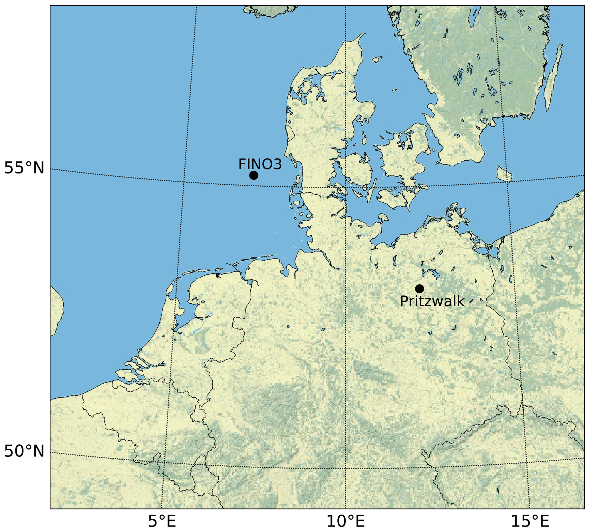
Figure 1Map of northern Germany with the representative onshore (Pritzwalk) and offshore (FINO3) locations highlighted by black dots.
The mesoscale simulations used the Weather Research and Forecasting (WRF) model (Powers et al., 2023). The onshore simulation was performed with version 3.6.1 (Skamarock et al., 2008) prior to the 2018 release of WRF version 4.0.2 (Skamarock et al., 2021), in which offshore simulations were computed. The setup of the model was adapted and constantly improved for wind energy applications by the authors of the present article for various projects and applications in recent years (Dörenkämper et al., 2015, 2017, 2020; Hahmann et al., 2020; Sommerfeld et al., 2019b). The focus of this study is not on the detailed comparison between mesoscale models but on AWES performance subject to realistic onshore and offshore wind conditions. Both WRF models provide adequate temporal and spatial resolution for preliminary performance assessment, despite the differences in setup and time frame.
Table 1Key setup parameters of the onshore and offshore mesoscale WRF simulations to generate the wind data used in this study.
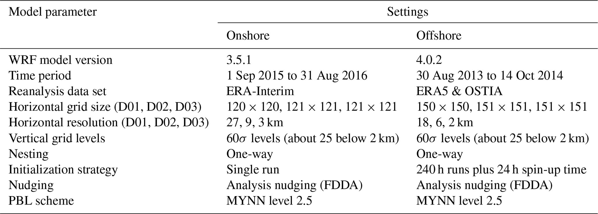
Each simulation consists of three nested domains around their respective location (black dot in Fig. 1). The innermost domain (D03) has the finest resolution and is nested within the middle domain (D02), which is nested within the outermost domain (D01) with the coarsest resolution. The simulations use one-way nesting where the outer domains define the boundary conditions for the inner domains. Atmospheric boundary conditions are defined by ERA-Interim (Dee et al., 2011) for the onshore location and by ERA5 (Hersbach and Dick, 2016) reanalysis data for the offshore location. Sea surface parameters for the offshore location, such as sea surface temperature and sea ice analysis, are based on OSTIA (Donlon et al., 2012). These data sets have proven to provide good results for wind-energy-relevant heights and sites (Olauson, 2018; Hahmann et al., 2020). Four-dimensional data assimilation (FDDA), also known as analysis nudging, nudges the simulation of the outer domain towards the atmospheric boundary conditions throughout the simulation time to reduce numerical drifting and provide smoother boundary conditions. Both simulations use the Mellor–Yamada–Nakanishi–Niino (MYNN) 2.5 (Nakanishi and Niino, 2009) level scheme for the planetary boundary layer (PBL) physics. The onshore simulation was carried out in a single 12-month simulation run from 1 September 2015 to 31 August 2016. The offshore simulation period covered a 410 d period from 30 August 2013 to 14 October 2014 and was divided into 41 simulations of 10 d each, with an additional 24 h of spin-up time per run. Spin-up is the period in which the model produces results that may not be reliable due to initialization using coarser global atmospheric reanalysis data. WRF calculates the vertical coordinate using a hybrid hydrostatic pressure coordinate, which is a function of surface and atmospheric pressure (Skamarock et al., 2021). Data at each vertical, terrain-following pressure coordinate (sigma level) are converted to geometric heights using the postprocessing methodology described by Dörenkämper et al. (2020). Table 1 summarizes the key model settings used in this study. All simulations were performed on the EDDY high-performance computing clusters at the University of Oldenburg (Carl von Ossietzky Universität Oldenburg, 2018).
2.2 Wind regime
Figure 2 depicts the wind roses of the computed annual wind conditions at 100 m (Fig. 2a and b) and 500 m (Fig. 2c and d) height onshore (left) and offshore (right). The dominant wind direction at both locations is southwest, turning clockwise with increasing altitude.
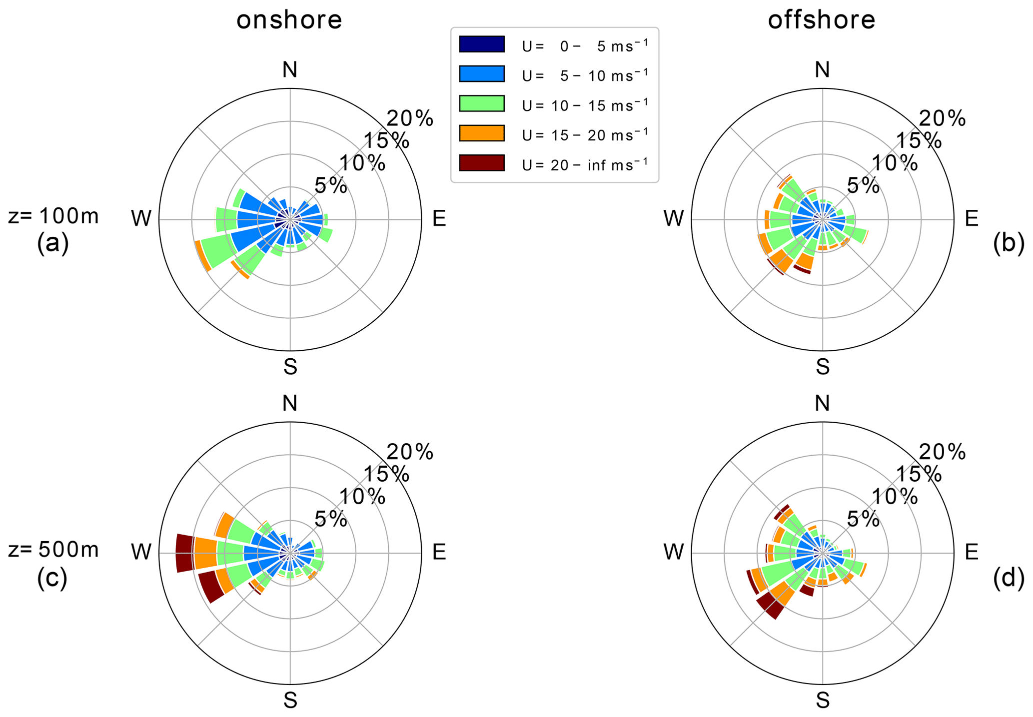
Figure 2Wind roses of annual wind direction and speed statistics at Pritzwalk (onshore) and FINO3 (offshore) for heights of 100 and 500 m during the simulated years.
Directional variability decreases, and the wind speed U, which is the magnitude of the wind vector U, increases with height, following the expected trends in the Northern Hemisphere (Arya and Holton, 2001; Stull, 1988). The average onshore wind direction turns about 14∘ between 100 and 500 m, whereas average offshore wind direction only veers approximately 5∘. The offshore wind direction turns approximately 10 additional degrees above 500 m, resulting in roughly the same westerly wind direction at around 1000 m. Due to the prevailing unstable conditions offshore accompanied by strong vertical mixing, the investigated heights show less veer than onshore. Wind shear at the offshore location is lower compared to the onshore location due to lower surface roughness.
Figure 3 shows the annual horizontal wind speed probability distributions at each height level for both locations. These distributions give insight into the wind statistics at specific heights but not into the statistics of the wind profile shapes. The nonlinear color gradient allows for the representation of the entire relative probability range. Onshore (Fig. 3a) U are relatively low and have a fairly narrow deviation below 300 m due to dominant surface effects. Above this height the distribution broadens, but a high probability of low wind speeds remains for the entire height range. The distributions show bimodal characteristics caused by different atmospheric stratification. Low wind speeds are commonly associated with unstable and high wind speeds with neutral or stable atmospheric conditions.
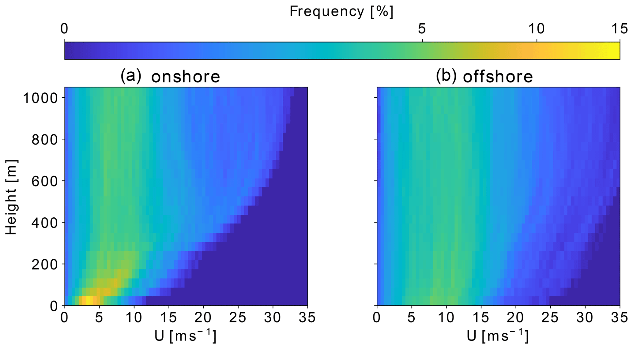
Figure 3Comparison of WRF-simulated annual wind speed U probability distributions at each height level between onshore (a) and offshore (b) up to 1000 m. The nonlinear color scheme represents the high probability of low altitude, particularly onshore, while still differentiating the lower, wide-spread frequencies at higher altitudes.
Such multimodal distributions at higher altitudes are better described by the sum of two or more probability distributions, as standard Weibull or Rayleigh distributions cannot capture this phenomenon (Sommerfeld et al., 2019a). Offshore U (Fig. 3b) display a wider distribution at all heights, as they are less affected by surface effects. Similarly to onshore, the offshore frequency distribution also shows a high probability of lower U (between 5–10 m s−1) at all heights. Higher U at lower altitudes benefit conventional WT and weaken the argument for offshore AWESs, as one of their benefits would be to harness energy from the stronger winds at higher altitudes. However, other reasons for placing AWES offshore are the safety and land use regulations and the potential cost benefits of a smaller support structure (offshorewind.biz, 2018; Lunney et al., 2017; Ellis and Ferraro, 2016).
The Obukhov length ℒ (Obukhov, 1971; Sempreviva and Gryning, 1996),
commonly characterizes the near-surface atmospheric stability, which highly affects the shape of the wind speed profile U, which is the magnitude of the wind velocity profile U. We extend the concept to mid-altitudes between 100 and 1000 m. The Obukhov length is a function of the simulated friction velocity u*, the virtual potential temperature θv, the potential temperature θ, the kinematic virtual sensible surface heat flux QS, the kinematic virtual latent heat flux QL, the von Kármán constant k, and the gravitational acceleration g. Various stability classifications based on the Obukhov length have been defined for different wind energy sites. Table 2 summarizes the Obukhov length bin widths used by Floors et al. (2011) and the frequency of occurrence of each stability class onshore and offshore, consistent with Sommerfeld et al. (2019b).
Table 2Stability classes based on Obukhov length ℒ (bins from Floors et al., 2011) and associated annual probability at Pritzwalk (onshore) and FINO3 (offshore), based on WRF simulations.
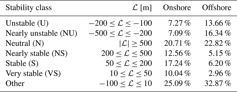
Neutral stratification occurs approximately 20 % of the year at both locations. The lower heat capacity of the land surface leads to a faster heat transfer and a quicker surface cool-off which favors the development of stable stratification (≈17 % onshore vs. ≈6 % offshore). The offshore location has a higher probability of unstable conditions, which is likely caused by a warmer ocean surface compared to the air above (Archer et al., 2016).
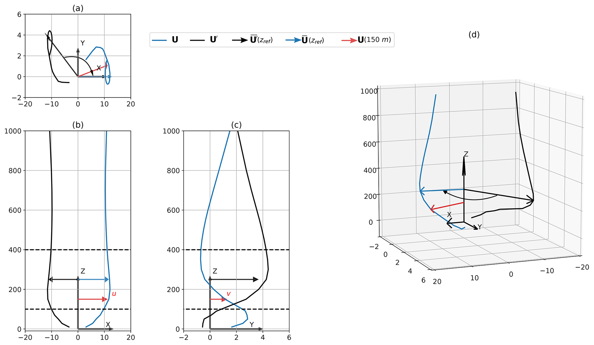
Figure 4Representative wind velocity profile U′ in its original direction and rotated so that the primary wind direction of the resulting profile U points in the x direction. Panel (a) shows the top view, panel (b) shows the front view, panel (c) shows the side view, and panel (d) shows the isometric view. The primary wind direction is defined by the average wind vectors (black) and (blue) between 100 and 400 m (dashed lines). As an example, the wind vector at z=150 m (red) (a, d) is decomposed into u and v (b, c).
Both unstable and stable conditions can lead to non-logarithmic and non-monotonic U profiles. Unstable conditions are often accompanied by almost uniform U profiles due to increased mixing, whereas low-level jets (LLJs) can develop during the nocturnal stable onshore boundary layer (Banta, 2008). Both locations have a high chance of unassigned conditions (labeled as “other”) which are mostly associated with low wind speeds.
2.3 Clustering of wind conditions
An accepted method to describe the near-surface atmosphere is atmospheric stability, commonly quantified by the Obukhov length (Obukhov, 1971; Sempreviva and Gryning, 1996), which exclusively uses surface data (Sect. 2.2 and Eq. 1). Previous studies (Sommerfeld et al., 2019a, b) showed that Obukhov-length-classified wind speed profiles U diverge with height, especially during neutral and stable conditions. This indicates vertically heterogeneous atmospheric stability and suggests that surface-based stability categorization is insufficient for higher altitudes. Unlike classifying wind regimes by atmospheric stability, which requires additional temperature and heat flux data, clustering only uses wind data at multiple heights to group profiles by similarity. This results in more cohesive profile groups (Schelbergen et al., 2020). Therefore, clustering can also be applied to wind-only measurements such as lidar.
The k-means clustering algorithm (Pedregosa et al., 2011) used in this study is chosen for its ease of use and scalability due to the high dimensionality of the data set. Many other algorithms produce similar results, but a comparison between clustering algorithms is beyond the scope of this research. The wind velocity profiles U′ (Fig. 4, black) are rotated such that the main wind component points in the positive x direction U (blue) in order to remove directional dependencies. The velocity components at each height level are decomposed into u in the main wind direction and into v perpendicular to it (red). The wind speed profile U is not shown. This results in more homogeneous clusters and simplifies the comparison of wind data and AWEBox results. It is analogous to assuming omnidirectional operation.
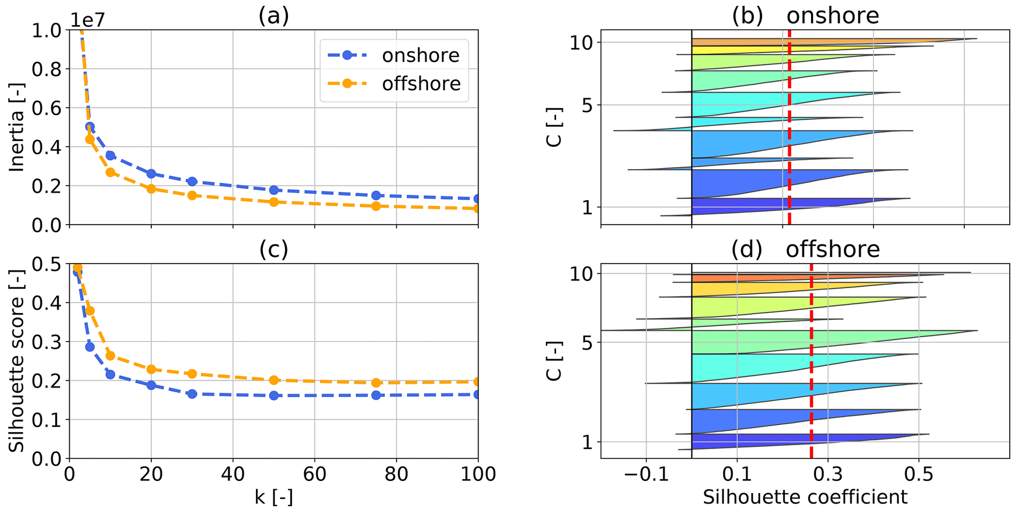
Figure 5The k-means clustering inertia over of number of clusters k (a) for 1 year of onshore (blue) and offshore (orange) wind velocity profiles U up to 1000 m. The onshore (b) and offshore (d) silhouette coefficients express the distance to neighboring clusters and are color coded according to average between 100 and 400 m, the same as in Figs. 6, 9, 10, and 11. The dashed red line represents the silhouette score, which is the average silhouette coefficient. Silhouette score (c) over number of clusters k for both locations. The number of clusters k=10 has been chosen for presentation purposes only. The analyses in the “Results and discussion” section use k=20 clusters.
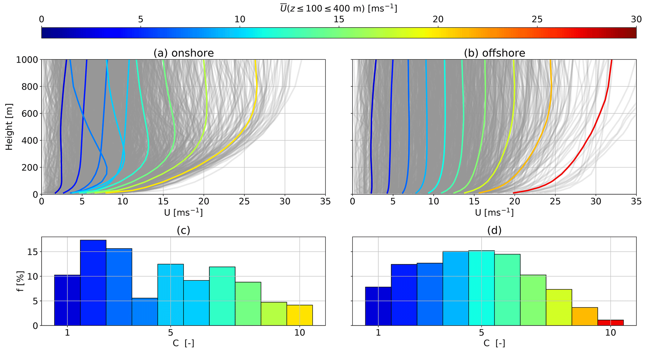
Figure 6Onshore (a, c) and offshore (b, d) average annual wind speed profiles (centroids) resulting from k-means clustering for k=10 (a, b). All WRF-simulated wind speed profiles U are depicted in gray. The centroids are sorted, labeled, and color coded in ascending order of average between heights of 100 and 400 m. The corresponding cluster frequency of occurrence f for each cluster C is shown in (c) and (d) below.
The wind velocity data up to 1000 m are comprised of data points at 30 height levels and in two directions. The clustering algorithm assigns each data point to one of the k clusters represented by their respective cluster mean, also called the centroid. These centroids are chosen to minimize the sum of the Euclidean distances to every data point within each cluster. This cost function is also referred to as inertia or within-cluster sum of squares. As such, the centroids are usually not actual data points, but rather the clusters' average, and will at best coincide with a data point by chance. The cluster labels are the result of random initialization and have no mathematical meaning. We therefore sort and label the clusters by average between 100–400 m for the following analyses in Sect. 2.4. The variable k refers to the fixed and predefined number of clusters. The choice of k significantly affects the accuracy of the wind resource description, as well as the computational cost. The choice of k is informed by the elbow method, named after the characteristic line chart that resembles an arm, and the silhouette score. The “elbow” (the point of inflection of the curve) is a good indication that the underlying model fits well for the corresponding number of clusters. k can be chosen at a point where the inertia reduction becomes marginally small or decreases linearly (Pedregosa et al., 2011).
Absolute values of inertia (Fig. 5a) are not a normalized metric and scale with the size of the considered data set. On the other hand, the silhouette coefficients (Fig. 5b and d) are normalized between −1 (worst) and 1 (best). They indicate the membership of a data point to its cluster in comparison to other clusters, i.e., the proximity of each data point in one cluster to data points in neighboring clusters (Pedregosa et al., 2011). A negative value suggests that a data point could be assigned to the wrong cluster. The silhouette score, depicted by a dashed red vertical line, is the average of all silhouette coefficients for a fixed number of clusters k. For visualization purposes, k=10 clusters have been chosen. Each cluster is sorted and color coded according to average between 100 and 400 m and color, the same as in Fig. 6. Performing these silhouette score analyses for multiple k results in the trend shown in Fig. 5c. A k value of 20 seems to be a good choice for the available data sets because the decrease in inertia for a higher number of clusters is only moderate, suggesting that the additional computational cost may not be worthwhile. Similarly, the silhouette score remains almost constant for higher numbers of clusters. Therefore, k=20 has been chosen for the analyses in Sect. 6.
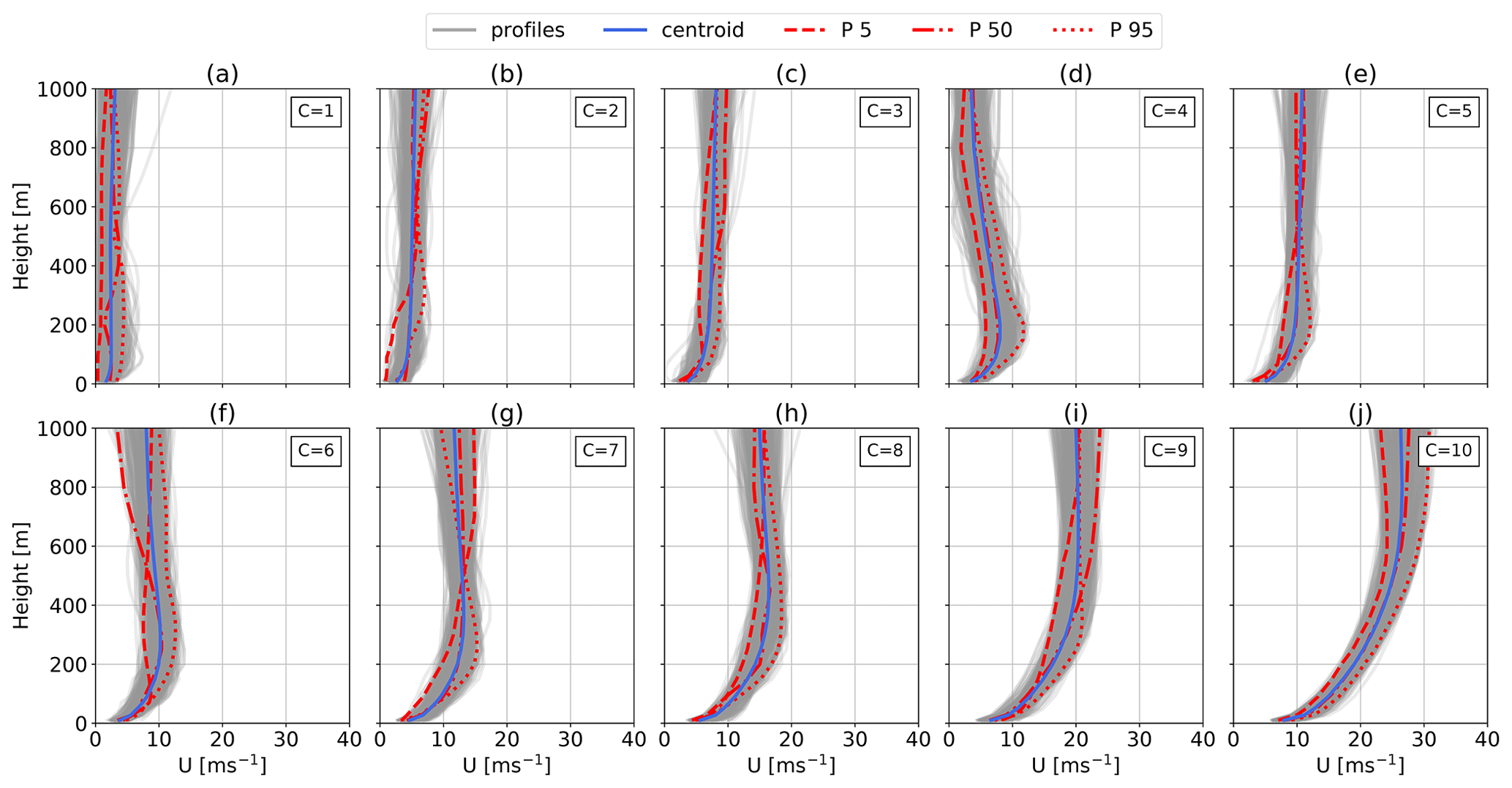
Figure 7Vertical onshore U categorized using the k-means clustering algorithm. The analyses in Sect. 6 employ k=20 clusters. Here k=10 is chosen for visualization purposes. The average profile (centroid) is shown in blue, and the profiles associated with this cluster are shown in gray. Clusters 1 to 10 (a–j) are sorted and labeled in ascending order of average centroid between 100 and 400 m. The corresponding cluster frequency f for each cluster C is shown in Fig. 6. The optimization-toolbox-implemented U are highlighted with a red line.
2.4 Analyses of clustered profiles
For visualization purposes, the following subsections describe the wind conditions at both locations using only k=10 clusters. The analyses in the “Results and discussion” section (Sect. 6) use k=20 clusters.
Figure 6a and b show the average of the clustered wind speed profiles U, also referred to as centroids. Their colors correspond to the average between heights of 100 and 400 m. All WRF-simulated U are depicted in gray. The cluster probabilities (Fig. 6c and d) are sorted by average centroid speed within the considered height range, represented by their colors and labels (C=1–10).
As expected, offshore U (Fig. 6b) at low altitudes are higher and wind shear is lower than onshore (Fig. 6a). In general, offshore centroids are more monotonic, as they do not exhibit a distinct U peak (i.e., LLJs), and achieve higher maximum wind speeds than onshore. The U profiles within each cluster cover a relatively small range, suggesting consistent clusters. Figure 7 (onshore) and Fig. 8 show the distribution of U within each of the clusters. At both locations, the first two clusters (Figs. 7a, b and 8a, b) exhibit very low wind shear with a low and almost constant U above 200 m. These low wind speed clusters amount to approximately 25 % onshore (Fig. 6c) and 20 % offshore (Fig. 6d), as can be seen in the corresponding cluster frequency of occurrence f. A standard logarithmic wind profile does not accurately describe such almost constant profiles which could lead to an overestimation of U at higher altitudes. AWESs must either be capable of functioning at low U or be able to safely land and take off autonomously. Onshore clusters 4 and 5 (Figs. 7d, e and 8d, e) seem to mostly consist of non-monotonic profiles, as these centroids show a distinct LLJ nose at about 200 and 300 m. The offshore centroids of clusters 7 and 8 (Figs. 7g, h and 8g, h) also show a slight wind shear inversion at higher altitudes.
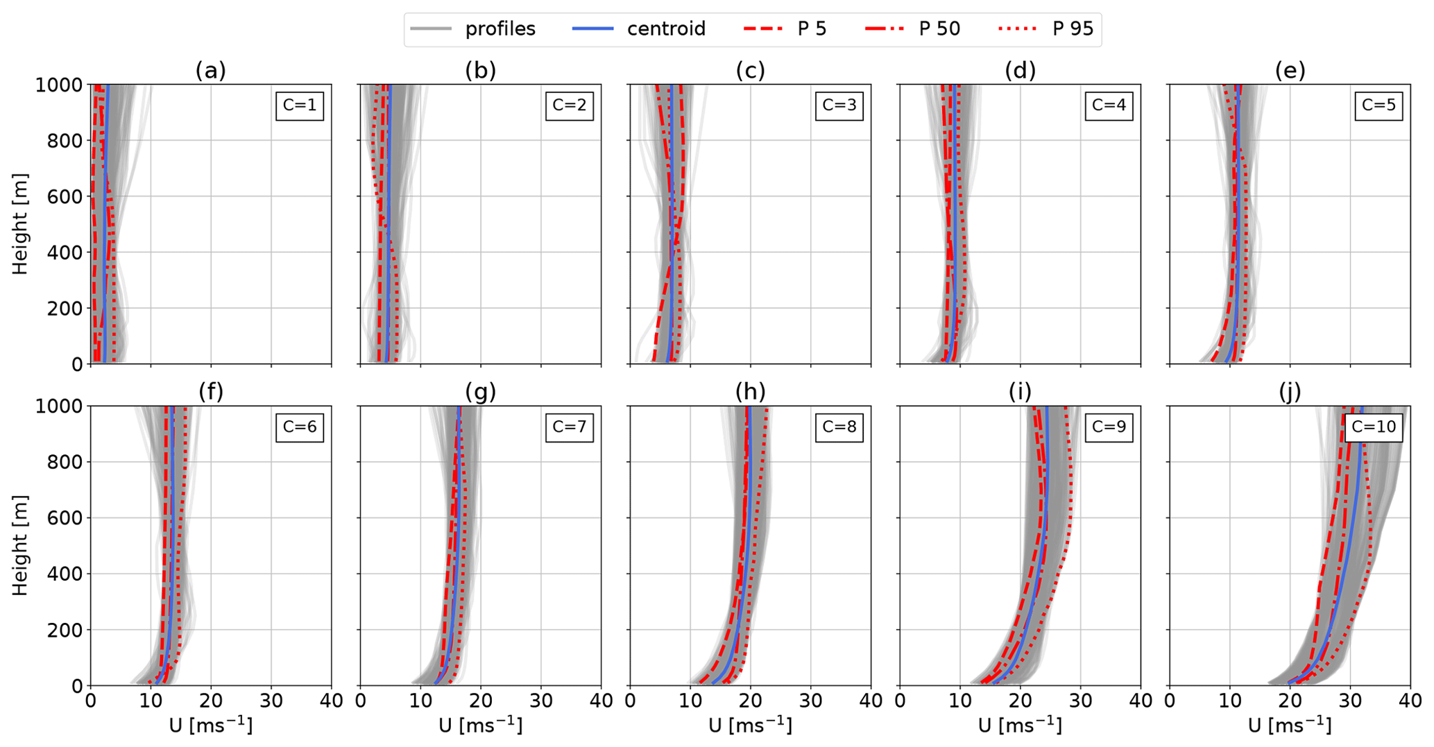
Figure 8Vertical offshore wind speed profiles categorized using the k-means clustering algorithm. The analyses in Sect. 6 employ k=20 clusters. Here k=10 is chosen for visualization purposes. The average profile (centroid) is shown in blue, and the profiles associated with this cluster are shown in gray. Clusters 1 to 10 (a–j) are sorted and labeled in ascending order of average centroid between 100 and 400 m. The corresponding cluster frequency f for each cluster C is shown in Fig. 6. The optimization-toolbox-implemented U are highlighted with a red line.
Clusters C=1 (a) to C=10 (j) are sorted by the average centroid (blue line) wind speed between –400 m).
The red lines indicate the profiles associated with the 5th, 50th, and 95th percentiles of within each cluster.
To reduce computational cost, only these profiles are later implemented into the AWEBox optimization toolbox. We selected these profiles because they are less likely to be irregular outliers than the extrema of the cluster while still representing the variation within their respective cluster. These profiles illustrate the variations within their respective cluster and are not average profiles like the cluster centroids or scaled or semi-empirical approximations such as the logarithmic wind profile.
Evidently, the magnitude of the wind speed plays a dominant role in the clustering process. A clearer wind profile shape distinction could be achieved by normalizing the data before clustering it (Molina-García et al., 2019; Schelbergen et al., 2020).
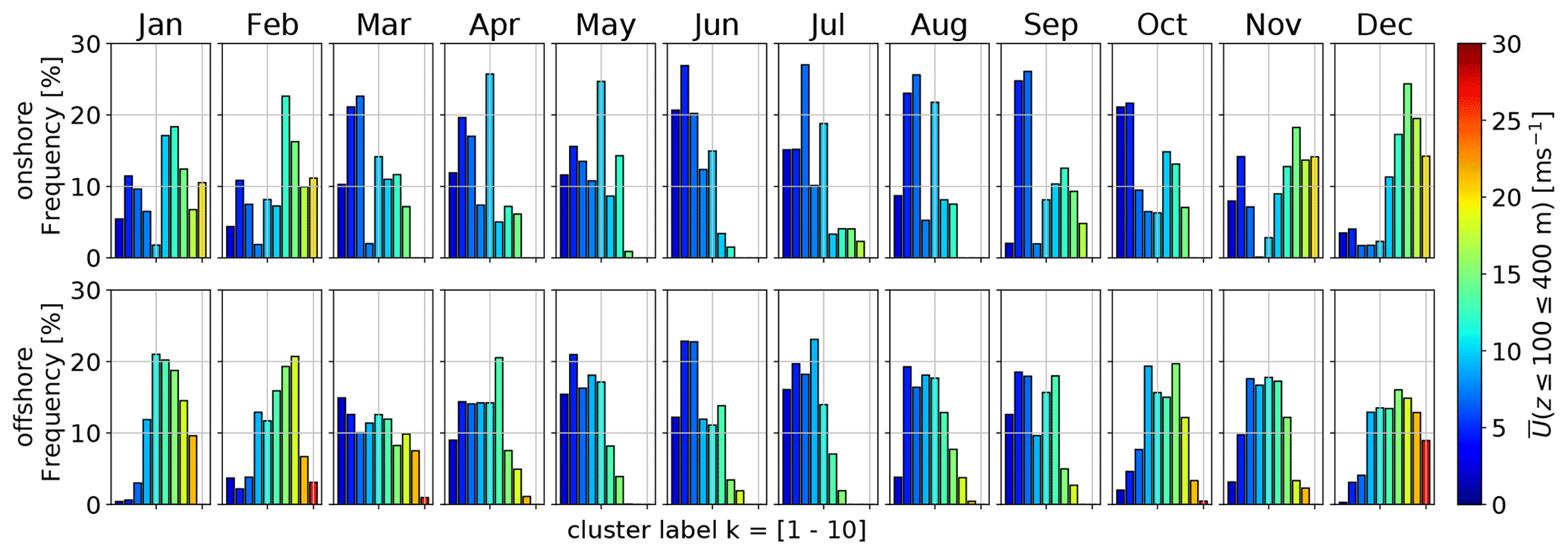
Figure 9Monthly frequency of k-means clustered onshore (top) and offshore (bottom) wind velocity profiles U for a representative k=10. All clusters are sorted and color coded according to their U(zref=100–400 m). The corresponding centroid associated with each cluster can be found in Fig. 6.
2.5 Analysis of clustered statistics
This subsection examines the relationship between the clusters and monthly, diurnal, and atmospheric stability. These analyses reveal patterns that give insight into the wind regime and the resulting changes in AWES performance. Subsequent sections examine wind data from k=20 clusters, while here only k=10 clusters are chosen for presentation purposes. Clusters are sorted in ascending order of average centroid wind speed –400 m) and color coded as in Figs. 5 and 6.
Both locations exhibit a clear annual pattern as shown in Fig. 9. High wind speeds are more common during winter, while low wind speeds are more prevalent in summer. This is likely due to the seasonal difference in surface heating and the resulting differences in atmospheric mixing. The two onshore and offshore clusters associated with the highest wind speed are almost exclusively present during November to February.
Offshore data indicate minimal diurnal variation as shown in Fig. 10, with only a slight increase in the frequency of lower-wind-speed clusters during the day. Onshore clusters, on the other hand, are more dependent on the diurnal cycle with a higher likelihood of low-speed clusters after sunrise. The frequency of onshore cluster 4, which includes a LLJ nose (Fig. 6), decreases to almost zero during the day and rises at night, supporting the notion that this cluster is linked to nocturnal LLJs.
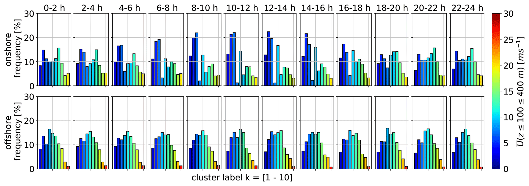
Figure 10Diurnal frequency of k-means clustered onshore (top) and offshore (bottom) wind velocity profiles U for a representative k=10. All clusters are sorted and color coded according to their U(zref=100–400 m). The corresponding centroid associated with each cluster can be found in Fig. 6.
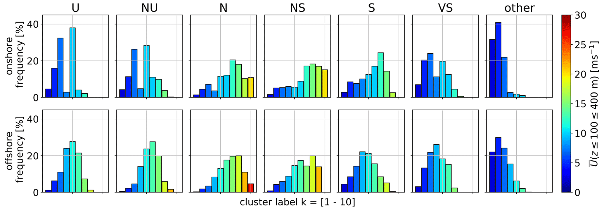
Figure 11Atmospheric stability (U: unstable; NU: nearly unstable; N: neutral; NS: nearly stable; S: stable; VS: very stable) distribution of k-means clustered onshore (top) and offshore (bottom) wind velocity profiles U for a representative k=10. The associated stability classes are based on Obukhov length (Table 2). All clusters are sorted and color coded according to their U(zref=100–400 m). The corresponding centroid associated with each cluster can be found in Fig. 6.
The wind velocity clusters (Fig. 11) show a correlation with atmospheric stability. Low wind speed clusters make up about 20 % to 30 % of the annual wind resource. These clusters exhibit Obukhov lengths close to zero (probably caused by very low friction velocity u*) and are classified as “other” according to Floors et al. (2011) (Table 2). Unstable (U) and near-unstable (NU) conditions are associated slightly higher wind speeds. The highest wind speeds develop during neutral (N) and near-stable (NS) conditions. It should be acknowledged that strong winds driven by large pressure gradients can lead to neutral stratification. LLJ profiles associated with onshore cluster 4 are most likely to develop during stable (S) and very stable (VS) conditions.
In summary, k-means clustering can effectively group wind velocity profiles with similar characteristics up to high altitudes. These clusters are correlated with seasonal and diurnal changes, as well as atmospheric stability. The magnitude of the wind velocity profiles appears to have a greater impact on the resulting clusters than the shape of the profile. The algorithm is able to identify non-monotonic profile shapes that are less common, including profiles with LLJs. Normalizing the profiles before clustering can provide more information about the different shapes of the vertical profiles, but this was not done in this study.
This section introduces the dynamic AWES model used in the AWEBox trajectory optimization toolbox (De Schutter et al., 2020). Section 3.1 provides a summary of the system configuration. The aerodynamic model is presented in Sect. 3.2, while the aircraft mass model is introduced in Sect. 3.3.
3.1 Model configuration
The rigid-body model considers a 6-degrees-of-freedom (DOF) fixed-wing aircraft which is connected to the ground via a straight tether. The introduction of the tether reduces the DOFs to 5 (Terink et al., 2011). The model uses precomputed second-order polynomials to describe the aerodynamic coefficients (Sect. 3.2) which are controlled via aileron, elevator, and rudder deflection (Malz et al., 2019).
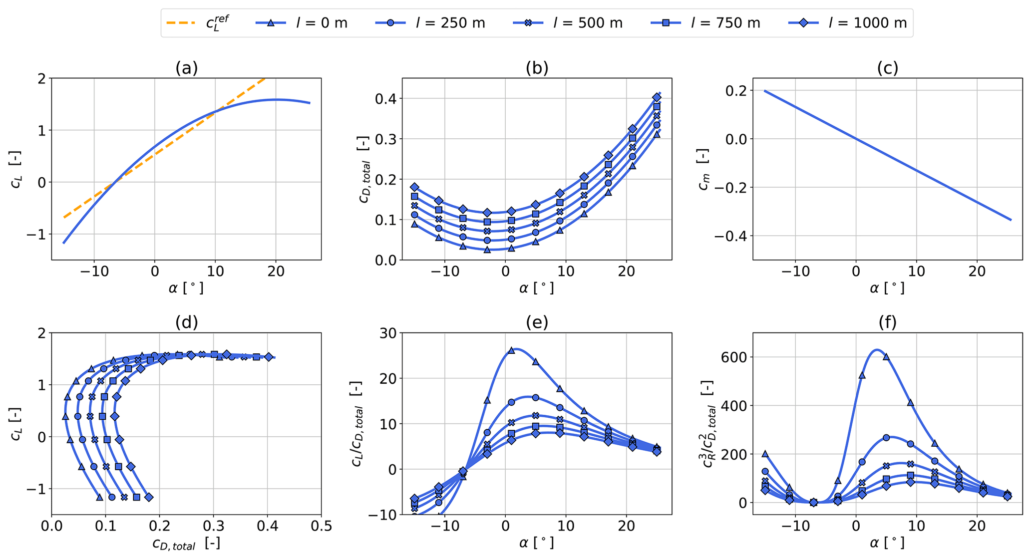
Figure 12Ampyx Power AP2 reference kite aerodynamic lift cL (a) and drag cD,total coefficients (b) (Malz et al., 2019; Ampyx Power BV, 2020), including tether drag according to Eq. (2), for a projected wing surface area A=20 m2 and tether diameter of d=7.8 mm. Tether length varies between 250 and 1000 m. Panel (c) shows the pitch moment coefficient cm as a function of angle of attack α. The bottom figures display lift over drag (d), glide ratio over angle of attack (e), and over angle of attack (f).
The longitudinal dynamics of the tether is controlled via the tether jerk from which the tether acceleration , reeling speed , and length l are determined. The tether is modeled as a single solid rod which supports neither compressive forces nor bending moments (De Schutter et al., 2019). The rod is divided into 10 segments. Tether drag is calculated individually for each segment, using the local apparent wind speed (Bronnenmeyer, 2018). The tether drag of every segment is equally distributed between the two endpoints. This leads to an underestimation of total tether drag at the kite (Leuthold et al., 2018). The ground station dynamics are not modeled explicitly but are implemented using a set of constraints. These constraints serve as an example of a system rather than representing a fully optimized design. A reel-in speed of m s−1 and reel-out speed of m s−1 are assumed to be realistic winch motor constraints based on information provided by a ground station manufacturer and literature review. This results in a reel-out to reel-in ratio of . A maximum tether acceleration of m s−2 is imposed to comply with generator torque limits. The tether diameter is selected to be able to withstand 3 times (safety factor of SF = 3) the maximum tether tension of kN. This results in a rated average cycle power of about Prated≈260–300 kW, according to AWEBox simulations.
3.2 Aerodynamic model
The presented model utilizes the Ampyx Power AP2 aerodynamic coefficients from De Schutter et al. (2020), Malz et al. (2019), and Ampyx Power BV (2020). The AP2 reference is scaled from a projected wing surface area of AAP2=3 m2 to A=20 m2 to generate results for more realistic and probable devices, while the aspect ratio is kept constant at AR=10. The total combined drag coefficient of the aircraft and tether cD,total,
depends on the diameter d and length l of the tether, as well as the projected surface area A and the aerodynamic drag coefficient cD,kite of the kite. To illustrate the effect of a longer tether, we utilize a simple tether drag estimation for a cylindrical tether with constant diameter and an aerodynamic tether drag coefficient cD,tether of 1.0. This value would be even higher for braided tethers. Assuming a constant and uniform wind speed, the line integral along the tether results in a total effective drag coefficient of and accounts for the different reference areas for cD,kite and cD,tether. See Houska and Diehl (2007), Argatov and Silvennoinen (2013), and van der Vlugt et al. (2019) for details. Figure 12 visualized the tether drag impact on the aerodynamic coefficients for tether lengths up to l=1000 m.
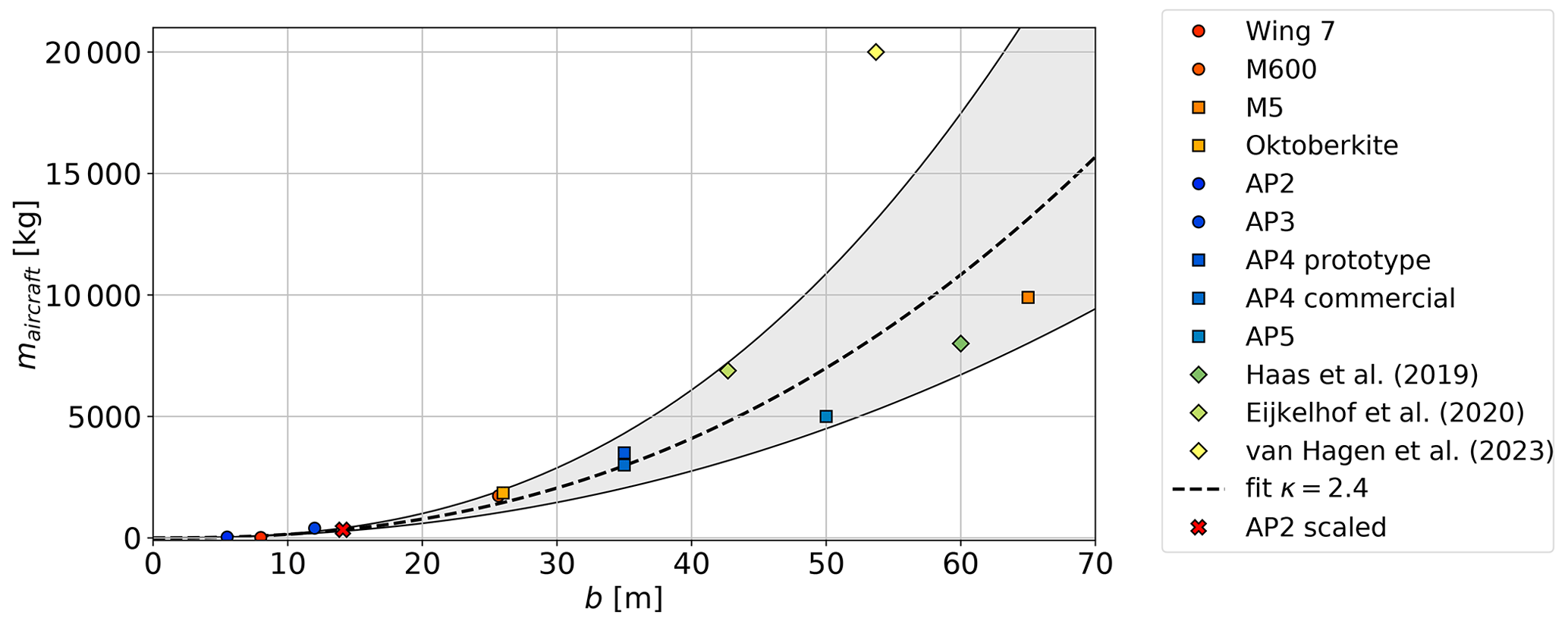
Figure 13Published actual (circle) and anticipated (square) aircraft mass scaling provided by Makani (red color scheme) (Echeverri et al., 2020) and Ampyx Power (blue color scheme) (Ampyx Power BV, 2020; Kruijff and Ruiterkamp, 2018). Diamond-shaped data (green color scheme) depict the mass of scaled-up versions of Ampyx Power prototypes used in research papers (Haas et al., 2019; Eijkelhof et al., 2020; van Hagen et al., 2023). For most data, mass scales with a scaling exponent between κ=2.2–2.6 (gray area). The chosen mass-scaling exponent of κ=2.4 is represented by a dashed line, and the investigated scaled AP2 design is highlighted by a red X.
The lift coefficient cL (Fig. 12a) is approximated as a second-order polynomial function of angle of attack α to simulate stall effects. A polynomial description is necessary for the entire range of angle of attack, as the optimization algorithm requires a two-times differentiable function. For the sake of simplicity, a piecewise, continuous, and differentiable function has not been implemented. As a result, the implemented cL (blue) slightly exceeds the linear (orange) lift coefficient of the AP2 reference (Malz et al., 2019) between ∘. The side slip angle β is included in the model, but variations in aerodynamic coefficients due to β are neglected. The pitch moment (Fig. 12c) is assumed to behave linearly. Changes in the drag coefficient (Fig. 12b) are approximated by a second-order polynomial. Tether drag is independent of α and therefore added to the zero-lift drag coefficient. The resultant aerodynamic force coefficient cR is represented as
The drag polar in Fig. 12d depicts the relationship between the kite's lift coefficient cL and total drag coefficient cD,total for the tethered aircraft. The maximum values of the glide ratio (Fig. 12e) and the ratio (Fig. 12f), which is one of the main determining factors of AWES power (Loyd, 1980; Schmehl et al., 2013), decrease significantly with tether length and shift towards higher angles of attack. The impact of tether drag on the total drag coefficient is less significant for larger kites because its impact decreases with the size of the aircraft.
3.3 Aircraft mass model
The aircraft dynamics are described by a single rigid body of mass mkite and moment of inertia J, subject to aerodynamic forces and moments. The inertial properties mkite and J are determined by upscaling the AP2 reference kite from AAP2=3 m2 to A=20 m2. The mass mscaled and moment of inertia Jscaled of a fixed-wing aircraft scale as functions of the wing span b and aspect ratio AR, which is kept constant and whose impact on scaling is neglected here, with a mass-scaling exponent κ (Noth and Siegwart, 2006):
Pure geometric scaling of solid bodies, in contrast to aircraft structures that use a lightweight structural frame, corresponds to Galileo's square–cube law with κ=3. In reality, as has been seen for the development of conventional WTs, design and material improvements occur over time. An appropriate mass-scaling factor was determined based on a review of the available literature. Figure 13 depicts actual (circle) and anticipated (square) aircraft mass scaling provided by Makani (red color scheme) and Ampyx Power (blue color scheme). The diamond-shaped data points (green color scheme) are scaled-up versions of Ampyx Power prototypes used in several research papers (Haas et al., 2019; Eijkelhof et al., 2020; van Hagen et al., 2023). The gray area encompasses most of the data points with κ=2.2–2.6. We chose κ=2.4 based on a curve fit of the available published sizing study data. This appears to be an ambitious goal for rigid kites but attainable for flexible ones. The mass of these hollow tensile structures filled with air mostly scales with the wing surface area, leading to significantly lower mass-scaling exponents and more beneficial mass scaling. Sommerfeld et al. (2022) examined the impact of various size, mass, and aerodynamic scaling factors on performance.
AWESs need to dynamically adapt to changing wind conditions to maximize power generation and ensure safe operation. Section 4.1 introduces the dynamic trajectory optimization toolbox AWEBox (De Schutter et al., 2020). We describe the most important boundary conditions in Sect. 4.2 and initial conditions in Sect. 4.3. Section 4.4 explains the implementation of the previously described wind profiles (Sect. 2).
4.1 AWES model overview
Maximizing the average cycle power can be formulated as a trajectory optimization problem, which takes into account the interaction between the tether, kite, and ground station. This study analyzes the mechanical power produced by a single aircraft tethered with a straight line throughout one production cycle, including reeling in and out, while disregarding take-off and landing. Power production is intrinsically linked to the aircraft's flight dynamics, as the AWES never reaches a steady state over the course of a power cycle. Generating dynamically feasible and power-optimal flight trajectories is nontrivial, given the nonlinear and unstable system dynamics and the presence of various flight envelope constraints. Optimal control methods are a natural candidate to tackle such problems, given their inherent ability to deal with nonlinear, constrained multiple-input–multiple-output systems (De Schutter et al., 2019; Leuthold et al., 2018). This trajectory optimization is a highly nonlinear and non-convex problem which can have multiple local optima. The initial and final states of each trajectory must be equal to ensure periodic operation but are freely chosen by the optimizer. In periodic optimal control, an optimization problem is solved by computing periodic system states and control inputs that maximize a performance index (here average power output ) while satisfying the system's dynamic equations and constraints. We use this approach to generate a variety of realistic trajectories from WRF-simulated wind velocity profiles. Any wind data sets, such as wind atlas data, lidar, or met mast measurements, can be implemented into the optimization model via a two-times differentiable function, depending on the scope and purpose of the investigation.
4.2 Constraints
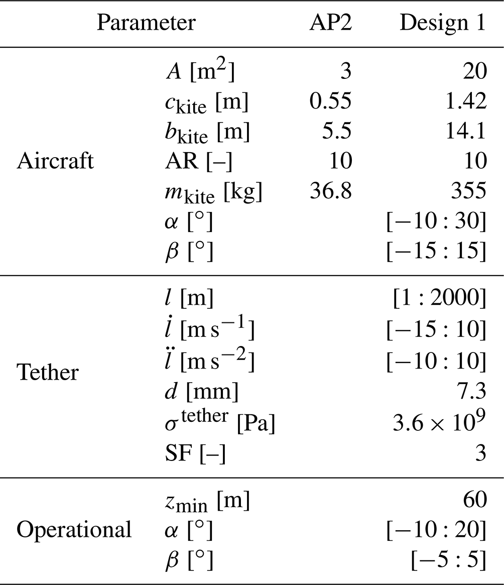
Several important constraints define the operational envelope. The most important constraints such as tether length, tether reeling speed, and tether force are summarized in Table 3. The following constraints define a representative and not design-optimized AWES. The power of a ground-generation AWES is limited by the tether force, which is defined by the tensile strength , tether diameter d, and the tether reeling speed . The tether diameter is chosen such that the maximum tether tension is approximately kN with an additional safety factor of SF = 3. This produces a peak power of Ppeak≈500 kW, with a maximum reel-out speed of m s−1. This corresponds to a rated average cycle power of approximately Prated≈260–300 kW. We assume a reel-out to reel-in tether reeling speed ratio of to be within winch design limitations. The tether length constraint is relatively lenient to allow the optimizer to investigate a wide range of possible operating heights zoper. The flight envelope is constrained by limitations on the aircraft's acceleration and roll and pitch angles (to prevent collision with the tether), as well as the angle of attack α and side slip angle β. A minimal operating height of is imposed for safety reasons.
Table 3Selected AWES design parameters for the original AP2 reference system (Malz et al., 2019) and the scaled-up A=20 m2 design analyzed in this study. Values in square brackets represent the upper and lower bounds, which are implemented as inequality constraints.
4.3 Initialization
The trajectory optimization process is highly nonlinear and non-convex, resulting in multiple local optima. These solutions depend on the chosen initial conditions. Some of the locally optimal solutions may be feasible and within the constraints but may have undesirable characteristics such as looping maneuvers during reel-in or excessively high operating altitudes.
As a result, it is necessary to evaluate the quality of all solutions. To solve the complex optimization problem, initial guesses are generated using a homotopy technique similar to Gros et al. (2013). This technique initially fully relaxes the dynamic constraints using fictitious forces and moments to reduce model nonlinearity and coupling, which improves the convergence of Newton-type optimization techniques. The constraints are then gradually re-introduced until the relaxed problem matches the original problem. The trajectory optimization is initialized with a circular trajectory in downwind direction (positive x direction) with a fixed number of nloop=5 loop maneuvers at a 30∘ elevation angle, an initial tether length linit=500 m, and an estimated aircraft speed of vinit=10 m s−1 along the entire initial trajectory.
This initialization is kept constant for all vertical wind velocity profiles.
The number of loop maneuvers is not part of the objective function and remains unchanged during all optimization runs. Further investigation is needed to determine the impact of the number of loops. However, previous analyses have shown that the average cycle power estimated by AWEBox is relatively unaffected by the number of loops. It is likely beneficial to reduce the number of loops with wind speeds because the system can reel out faster at higher wind speeds and reach maximum tether length faster.
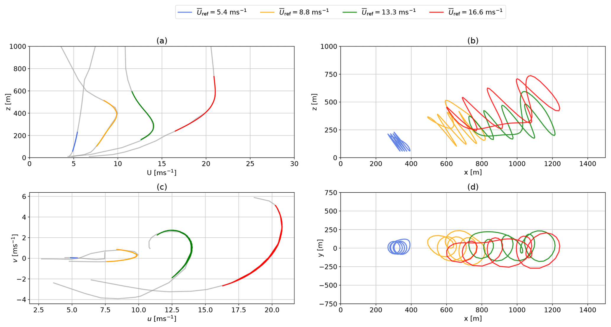
Figure 14Representative WRF-simulated vertical onshore wind speed profiles U (a) and hodograph (top view) up to 1000 m (c). The highlighted sections indicate Lagrangian polynomial fit of the wind velocity at operating height. Panel (b) and panel (d) show the side and top view of the corresponding AWEBox-optimized trajectories.
The reference wind speed in the legend is .
The results correspond to the time series shown in Fig. 16.
4.4 Wind profile implementation
To reduce the computational cost while maintaining an adequate representation, we only implement three wind velocity profiles from each cluster into the trajectory optimization toolbox. More profiles could be chosen for an in-depth analysis. The power for a total number of 60 wind profiles, three profiles for each of the k=20 clusters (Sect. 2.3), for each location is maximized. The three selected profiles correspond to the 5th, 50th, and 95th percentiles of average wind speed –400 m) within each cluster. We assume that these profiles represent the cluster's spectrum of wind conditions at operating height zoper. The AWEBox includes a simplified atmospheric model based on international standard atmosphere to account for the variation in air density.
The vertical wind velocity profiles U′ are rotated such that the main wind direction, which is defined as the average direction between 100 and 400 m, points in the positive x direction (Fig. 4). As a result the wind velocity components at every height consist of a main component u in the x direction and transverse component v in the y direction. The results can be seen in the hodographs of Figs. 14c and 15c.
The AWEBox toolbox uses the gradient-based MA57 solver (HSL, 2020) in IPOPT (Waechter and Laird, 2016) to solve the nonlinear control problem. Therefore, it is necessary to interpolate the vertical wind velocity profiles with a two-times continuously
differentiable function. We chose to use Lagrangian polynomials (Abramowitz and Stegun, 1965) because the resulting polynomials pass through the input data points. To avoid over-fitting a limited number of data points are implemented. These data points are chosen based on the anticipated zoper to best represent the wind conditions at relevant heights.
For comparison, logarithmic wind speed profiles,
with a roughness length of and are implemented into the trajectory optimization toolbox.
The reference wind speed U10 at the reference height z10=10 m varies from 3 to 20 m s−1 with a step size of ΔU10=1 m s−1.
This section introduces a simplified quasi-steady-state AWES reference model (QSM) (Sect. 5.1) and a steady-state WT model (Sect. 5.2). The so generated analytical solutions will serve as a reference for the optimization results.
5.1 AWES reference model
The QSM estimates the mechanical power of ground-generation AWES based on the assumption that the trajectory of the tethered aircraft can be approximated by a progression through steady equilibrium states where tether tension and total aerodynamic force are aligned. We simplify the QSM by approximating the reel-out and reel-in trajectory with a single state and neglecting the effects of gravity. The QSM, based on Argatov et al. (2009) and generalized by Schmehl et al. (2013) and van der Vlugt et al. (2019), approximates the aircraft as a point mass. Its position is described in terms of spherical coordinates, i.e., the radial distance from the ground station, the elevation angle ε, and azimuth angle ϕ relative to the direction of the mean wind velocity vector U. For lightweight soft-wing kites, this is a reasonably good approximation because the low mass of the kite leads to very short acceleration times. The model includes losses caused by the misalignment of the tether and the wind velocity vector. The same design parameters, system constraints, and wind conditions (Sect. 2) apply to the optimization model (Sect. 4.2), as well as the QSM reference model. We maximize the cycle average power PQSM by varying l, and z and assuming an optimal ratio .
The average cycle power PQSM,
can be estimated from the reel-out power Pout, the power losses during reel-in Pin, the reel-in time tin, and reel-out time tout. We assume reel-in power losses Pin to be zero because optimal reel-in tether tension is negligible. This reduces the average cycle power by up to 30 %, depending on wind speed. Due to the cyclic nature of the trajectory, we can determine the ratio of the reel-in time tin and reel-out time tout to the total cycle time ttotal from the reel-in speed and reel-out speed . depends on the wind speed, while m s−1 is assumed to be the maximum reel-in speed.
During the reel-in and reel-out phases, we assume that the tether force Ftether and reeling speed remain constant. The time it takes to transition between these two phases is not taken into account. Pout is calculated from the product of tether reeling speed and tether tension Ftether:
Tether tension is a function of the apparent wind speed Uapp, air density ρ, and the resultant aerodynamic force coefficient cR (Eq. 3). The apparent wind speed can be nondimensionalized by
The tether reeling speed is nondimensionalized by defining the reeling factor:
The elevation ε and azimuth angle ϕ constrain f≤cos εcos ϕ because the magnitude of the apparent wind speed cannot be negative. Combining Eqs. (8) and (10) results in
The optimal reeling factor can be obtained from Eq. (11) through an extreme value analysis. We assume an average reel-out trajectory represented by a single crosswind state instead of tracking the actual trajectory. The trajectory center is aligned with the main wind direction (ϕ=0∘). The elevation angle ε is determined using the tether length l and operating height zoper. Ftether is constrained by the tether diameter d, the tensile strength , and the safety factor SF:
The power-harvesting factor ζ (Diehl, 2013) is an AWES performance metric:
The harvested power P is expressed relative to the kinetic wind energy flow rate Parea, Parea being a mathematical concept rather than a physical power flux, through an area equivalent to the wing surface area A to nondimensionalize the power. ζ can be derived from Eq. (8) by setting the elevation angle ε and the azimuth angle ϕ to zero.
5.2 WT reference model
This section introduces a simplified steady-state reference WT model that calculates power as
with a hub height of zWT=100 m for both onshore and offshore conditions. The rotor diameter DWT≈26.9 m is sized such that an equivalent rated power of Prated=260 kW is reached at a rated wind speed of m s−1, assuming a constant power coefficient of . The power is kept constant above the rated wind speed. The performance of the WT model, dynamic optimization toolbox, and QSM is estimated using the same sampled WRF-simulated wind conditions (Sect. 2).
This section analyses the optimization results and compares them to the reference models. Section 6.1 investigates power-optimal trajectories and the time series of operational parameters. Section 6.2 examines operating height statistics, tether length, and elevation angle trends. Section 6.3 visualizes the impact of wind speeds at different reference heights on the power curve. We compare three different wind speeds: the wind speed at a reference height of 100 m , the average wind speed at pattern trajectory height , and the average wind speed at an a priori guess of pattern trajectory height . The investigated power curves do not represent design-optimal performance. Section 6.4 examines the variation in average cycle power caused by realistic wind profiles simulated by WRF and compares them to reference power estimates based on logarithmic profiles. All results are subject to the same constraints and design parameters introduced in Sects. 3 and 4.
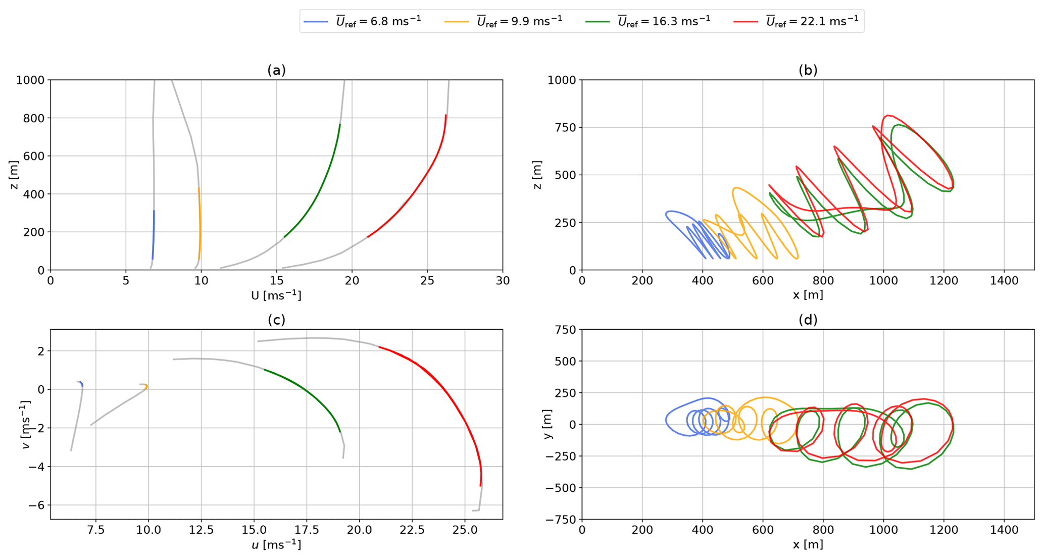
Figure 15Representative WRF-simulated vertical offshore wind speed profiles U (a) and hodograph (top view) up to 1000 m (c). The highlighted sections indicate Lagrangian polynomial fit of the wind velocity at operating height. Panel (b) and panel (d) show the side and top view of the corresponding AWEBox-optimized trajectories.
The reference wind speed in the legend is .
The results correspond to the time series shown in Fig. 17.
6.1 Flight trajectory and time series results
Figure 14 compares representative onshore and offshore power-optimal flight trajectories. These results have been chosen to visualize typical performance-optimized trajectories for realistic wind conditions determined with the AWEBox. The reference wind speed in the legend is the average wind speed at the a priori guess of the pattern trajectory height .
Figure 14a shows the magnitude of the vertical wind velocity profile U. Figure 14c shows the corresponding top view of the wind velocity profile, rotated such that the main wind component (average wind direction between 100 and 400 m) u points in the positive x direction. The WRF-simulated wind profiles are shown in gray. The highlighted segments depict the Lagrangian polynomial fit (Abramowitz and Stegun, 1965) at operating heights. These polynomials that have been incorporated into the optimization toolbox provide a sufficient fit for the wind data. Figure 14b and d show a side (x–z plane) and top view (x–y plane) of the optimized trajectories. The optimization predicts an increase in tether length, operating height, and stroke length with wind speed. Figure 15 shows similar results for the offshore location. Figure 16 illustrates the corresponding temporal development of important operational parameters.
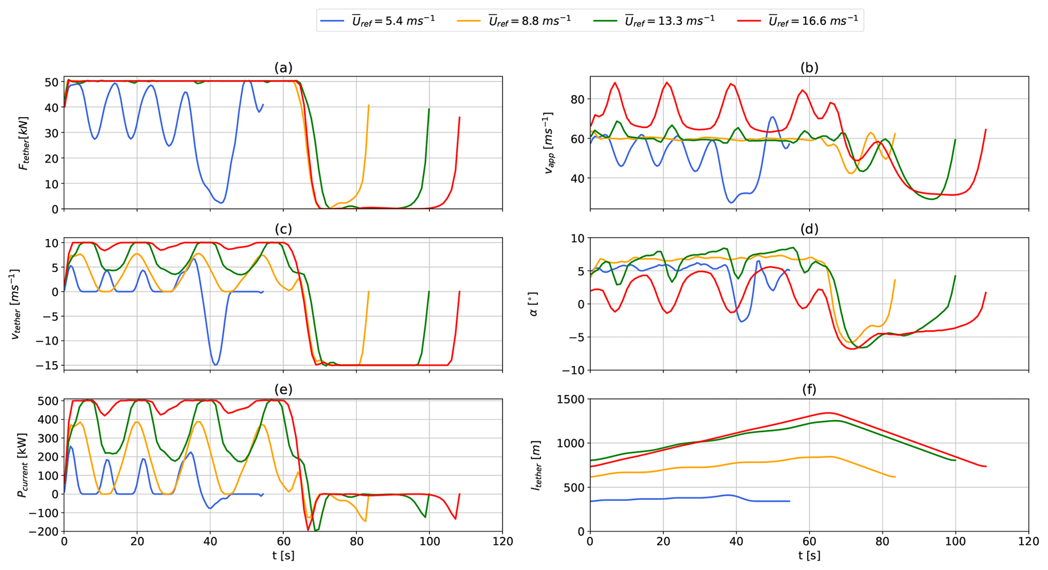
Figure 16Time series of instantaneous tether tension (a), apparent wind speed (b), tether-reeling speed (c), angle of attack (d), power output (e), and tether length (f) over one pumping based on representative onshore WRF-simulated wind data. The results correspond to trajectories shown in Fig. 14.
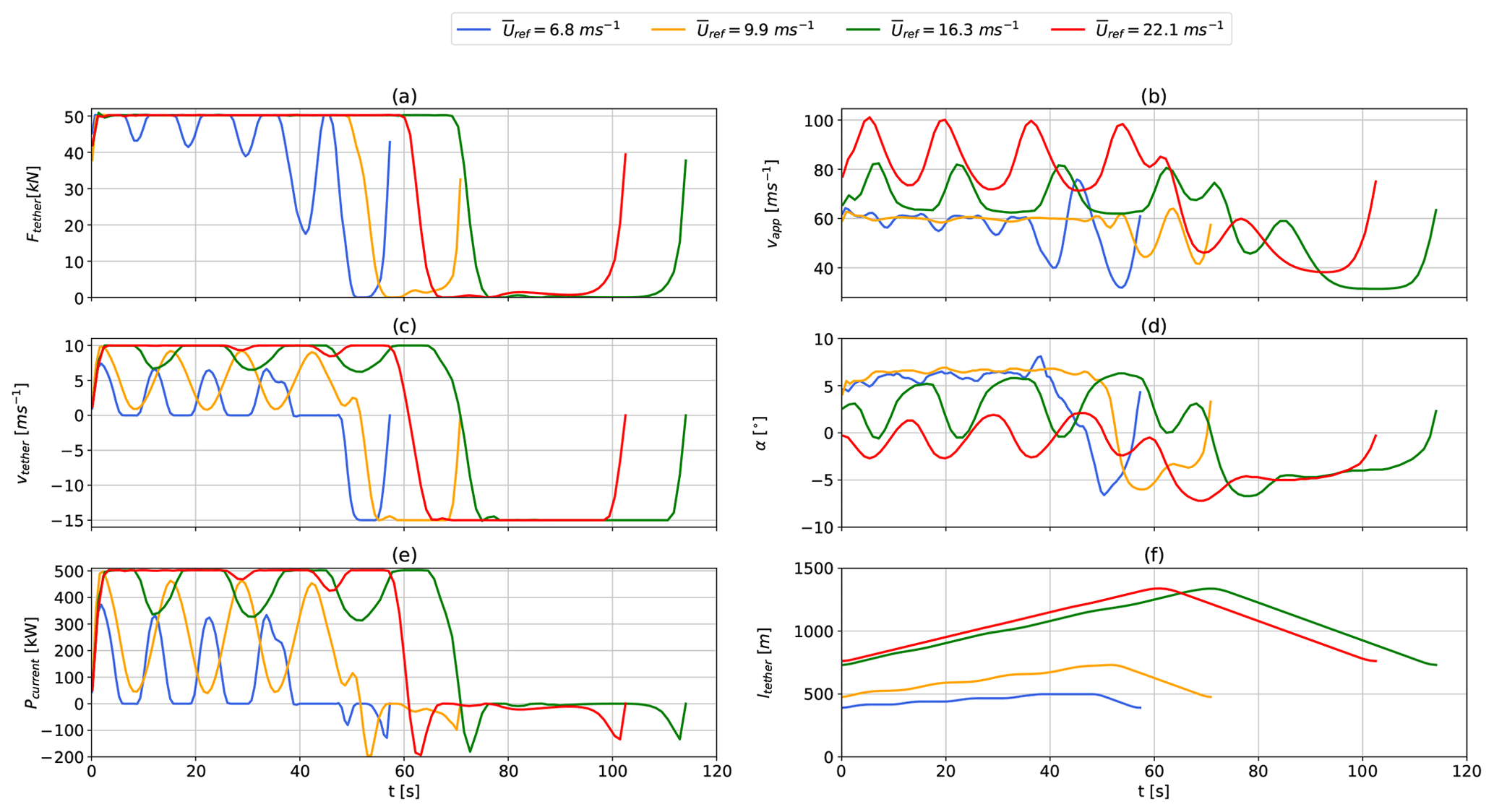
Figure 17Time series of instantaneous tether tension (a), apparent wind speed (b), tether-reeling speed (c), angle of attack (d), power output (e), and tether length (f) over one pumping based on representative offshore WRF-simulated wind data. The results correspond to trajectories shown in Fig. 15.
The optimizer maximizes tether tension by adjusting the reel-out speed and angle of attack (Fig. 16a) during reel-out even for lower wind speeds and adjusts the reel-out speed (Fig. 16c) to maximize average cycle power. This causes the reeling factor to exceed its optimal value of at high wind speeds, resulting in an increase in power (Fig. 16e) even when the maximum tether force has been reached. The low-wind-speed example m s−1 (blue) seems to be just above cut-in wind speeds. The tether reeling speed decreases to zero for a prolonged period during the reel-out phase in order to generate enough lift to keep the aircraft aloft. The production period remains almost constant (t≈60 s) for the moderate- and high-wind-speed trajectories (orange, green, and red), while the reel-in period increases with wind speed due to the increased reel-out length caused by a higher average reel-out speed. There are significant power losses during the transition between the production and retraction phases when the tether is reeled in, and the tension remains high because the aircraft is unable to de-power quickly enough. During the reel-in phase, the tether reeling speed reaches its limit and the tether tension decreases to zero. This happens as the aircraft reduces its angle of attack and lift, as shown in Fig. 16d. At higher wind speeds the optimizer increases the elevation angle and reduces angle of attack to stay within the constraints. This can result in odd or unexpected trajectories, even though these local minima are feasible solutions within the system constraints. Tether length (Fig. 16f) generally increases with wind speed as the system reels out faster, increases its elevation angle, and operates at higher altitude. Similar results for the offshore location are shown in Fig. 17.
6.2 Tether length, elevation angle, and operating altitude
Figure 18a illustrates the range of tether lengths l for each of the 60 onshore (blue) and offshore (orange) wind velocity profiles. The maxima and minima are highlighted by circles and plotted over the reference wind speed –400 m).
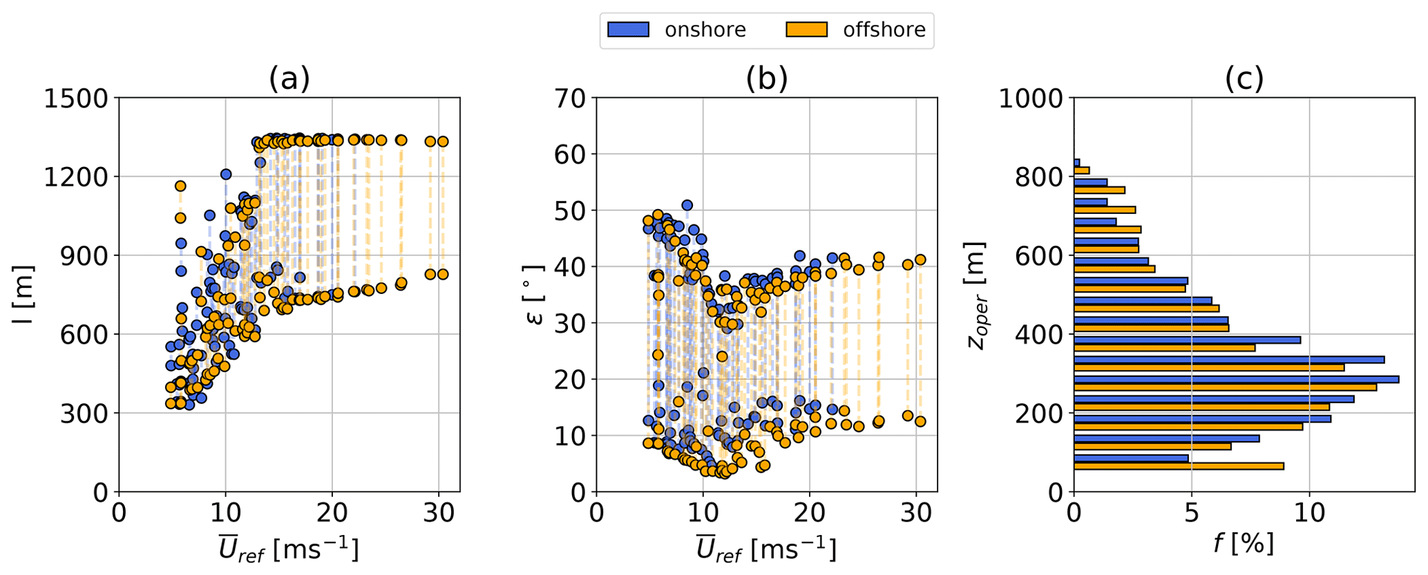
Figure 18Tether length range (a) and frequency distribution of operating height zoper (b) over reference wind speed U(zref=100–400 m) based on AWEBox trajectory optimizations of k=20 onshore (blue) and offshore (orange) clusters.
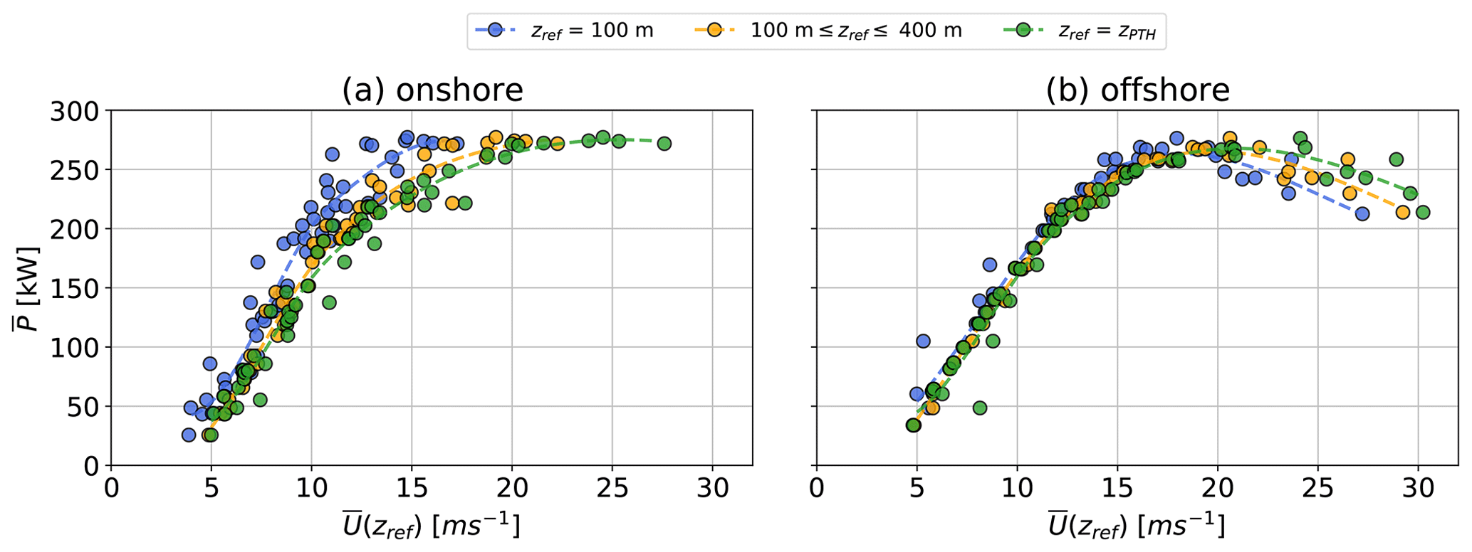
Figure 19Onshore (a) and offshore (b) AWES power curve approximations with wind speeds at zref=100 m (blue), (orange), and zref=zPTH (green) reference heights. The dashed lines represent least-square spline interpolations that have been added to aid in visualization.
None of the optimizations reach the maximum tether length constraint of lmax=2000 m because a longer tether would not be advantageous due to the added drag and weight, which would decrease performance. Both locations show a trend towards longer tethers up to rated wind speed, where the reel-out speed and tension are almost constant and close to their respective constraint (Fig. 16). The maximum tether length remains almost constant above rated wind speed, while the minimum tether length increases slightly, reducing the total stroke length. The elevation angle (Fig. 18b) decreases as the tether length increases. The optimizer tries to keep the elevation angle low in order to reduce misalignment (cosine) losses between the tether and the wind velocity vector. The onshore elevation angle is slightly higher because of the increased wind shear, which makes higher operating altitudes more justifiable. This can also be seen in Fig. 18c which shows the frequency distribution of operating altitude. Of the optimal operating heights, 78.6 % onshore and 74.7 % offshore are below 400 m, confirming the findings in Sommerfeld et al. (2019a, b). Larger or multikite AWESs could benefit from higher operating altitudes due to their higher lift to tether drag ratio and lift to tether weight ratio, but more detailed analyses are required.
6.3 Impact of reference height on power curve
The power curve of wind energy converters quantifies the power that can be harvested at a given reference wind speed. For conventional WTs the wind speed at hub-height is commonly used as the reference wind speed. Whether this is appropriate for ever-growing towers and longer rotor blades is debatable (Van Sark et al., 2019; Wharton and Lundquist, 2012; European Wind Energy Association, 2012). Defining a reference wind speed for AWES is not trivial, as the operating height depends on the shape and magnitude of the vertical wind speed profile. The choice of reference wind speed impacts the power curve representation. The AWE glossary (Airborne Wind Europe, 2021) recommends using the wind speed at pattern trajectory height zPTH, which is the expected or logged time-averaged height during the power production phase, as the reference wind speed. We estimate as an a priori guess of the pattern trajectory height. Figure 19 compares onshore (Fig. 19a) and offshore (Fig. 19b) average cycle power over U(zref=100 m) (blue), (green), and an a priori guess of the wind speed at pattern trajectory height (orange).
Each data point corresponds to one of the sampled WRF-simulated wind velocity profiles U. The dashed lines, which are only added as visual aid, are a least-square spline interpolation of the approximately 60 data points. Based on these results, we can conclude that the selection of the reference height is more important for onshore conditions. The onshore wind conditions with their higher number of non-monotonic wind profiles and higher wind shear lead to larger deviations from the typical power curve shape described in Licitra et al. (2019), Airborne Wind Europe (2021), and others. The higher wind shear onshore leads to a shift towards lower wind speeds for a reference height of zref=100 m. The a priori pattern trajectory height guess of is relatively close to the actual zPTH, especially for lower wind speeds. At very high wind speeds above m s−1 the zPTH power shifts towards higher wind speeds indicating an increased operating height.
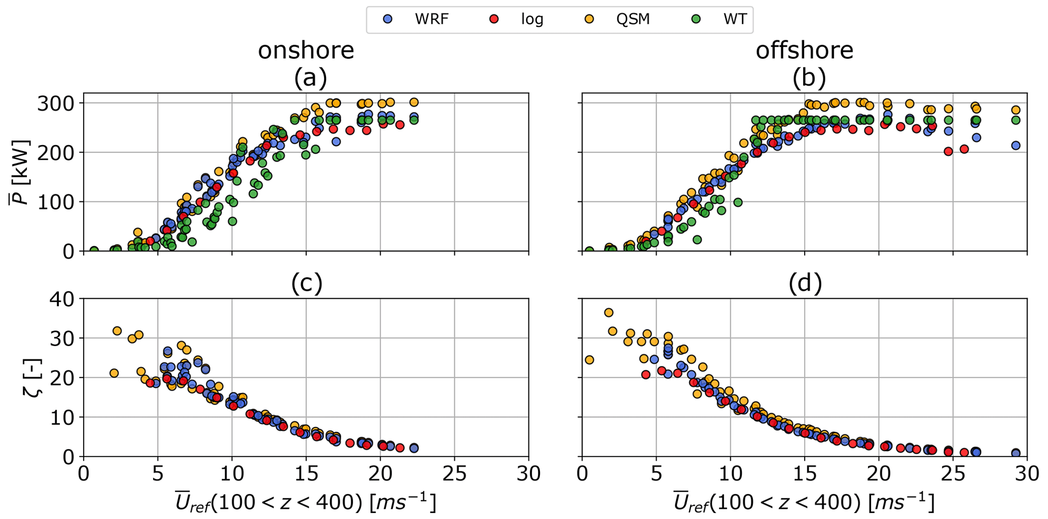
Figure 20Average cycle power and power-harvesting factor ζ for the onshore (a, c) and offshore (b, d) locations as a function of average wind speed between 100 and 400 m. The data points obtained from AWEBox (blue), QSM (orange), and the WT model (green) are based on WRF wind data and are compared to AWEBox data derived from standard logarithmic wind speed profiles (red).
The more homogeneous offshore wind conditions result in less power variation.
The three different reference heights have almost no impact on the offshore power curve up to the rated wind speed. Above m s−1 the power curves diverge and the average cycle power decreases. This seems to be a result of the AWEBox optimization and its initialization with a fixed number of loop maneuvers. As the wind speed and reel-out speed increase, the aircraft cannot complete all the loop maneuvers before reaching the maximum tether length and transitioning into reel-in. Therefore, one of the loop maneuvers is performed when already reeling in, leading to an increase in tether tension (Fig. A1a) and additional losses during the reel-in period (Fig. A1e).
The corresponding trajectories are shown in Fig. A2.
6.4 Reference model power comparison
Figure 20 compares the variation in the power curve for a reference wind speed of based on sampled WRF-simulated wind data (blue) and power estimates based on standard logarithmic wind speed profiles (red). These results are verified against the QSM (Sect. 5.1, orange) and WT reference models (Sect. 5.2, green).
The QSM and WT reference model use the same sampled WRF-simulated wind data. No cut-out wind speed is defined. The cut-in wind speed of m s−1 is the result of unconverged optimizations. The optimization algorithm was not able to find a feasible trajectory for these low wind speeds, indicating that the wind is insufficient to keep the AWES aloft and produce power. The QSM and WT model estimate power for these wind speeds. Rated power is achieved around Urated≈12–15 m s−1, depending on the wind speed profile shape. At these wind speeds the reel-out speed is almost constant, while a constant reel-out tension is already achieved at lower wind speeds (Fig. 16).
The logarithmic wind speed profiles (Eq. 6) use roughness lengths of and . Onshore, the power predicted based on WRF wind data is often higher than the power predicted using logarithmic profiles (Fig. 20a). This is likely due to higher than predicted wind shear and the presence of LLJs that are not represented by logarithmic profiles. Offshore, the logarithmic and WRF data are in close agreement with the logarithmic results because most of the simulated wind profiles are more monotonic.
The ζ trends for both onshore (Fig. 20c) and offshore (Fig. 20d) conditions show a decrease with increasing wind speed and are consistent with the QSM. WT power fluctuates due to the choice of reference height. AWESs outperform WTs up to rated wind speed, particularly onshore where AWESs can take advantage of higher wind speeds aloft. Lower wind shear offshore reduces the need to operate at higher altitudes, reducing the benefit of AWESs. The QSM predicts the highest power, as anticipated, due to its simplified assumptions such as constant power during reel-out and reel-in and neglected mass.
This research compares the optimal performance of a single-aircraft, ground-generation AWES using mesoscale wind data simulated by the WRF model to the performance calculated using standard logarithmic wind profiles. It also describes trajectories, instantaneous performance, and trends in tether length and operating height. These analyses use 1 year of onshore wind data at Pritzwalk in northern Germany and 1 year of offshore wind data at the FINO3 research platform in the North Sea to drive the AWEBox optimization, which determines dynamically feasible, power-optimal trajectories. The annual wind data are categorized into k=20 clusters of vertical wind velocity profiles U using a k-means clustering algorithm. To decrease the computational expense, three profiles based on the 5th, 50th, and 95th percentiles of wind speed between for each cluster are incorporated into the performance optimization model.
The performance model uses a scaled Ampyx Power AP2 aircraft with a wing surface area of A=20 m2 and is subject to realistic tether and operational constraints. Our investigation into the impact of wind speed at reference height found that the a priori guess of m is a good guess for the investigated AWES design and size. Optimal average cycle power is compared to a quasi-steady-state AWES model and a steady-state WT model.
The optimization model is able to determine power-optimal trajectories for complex, non-monotonic wind velocity profiles. The optimized results are only marginally lower than those obtained using the simplified QSM, which neglects the effects of gravity and only simulates a single reel-in and reel-out state instead of the entire trajectory. The predicted onshore AWES power exceeds the WT reference model. This is because AWES can adapt their operating altitude to benefit from higher wind shear or LLJs. Offshore wind velocity profiles are generally more monotonic and exhibit higher wind speeds with less turbulence and wind shear. As a result, offshore winds produce average power that is similar to their logarithmic approximation. Due to the initialization of the AWEBox with a fixed number of loop maneuvers, which is not a variable in the objective function, high-wind-speed trajectories show loops during the reel-in period which reduce the average cycle power. This can lead to a deterioration of the trajectory at high wind speeds, as the optimizer struggles to stay within the tether tension and tether reeling speed constraints.
An investigation of the time series data shows that the optimizer first maximizes tether tension by adjusting reel-out speed and angle of attack. As the wind speed increases, the tether reel-out speed approaches its maximum limit and becomes more constant, whereas at lower wind speeds, the reel-out speed varies more. Up to rated wind speed, when average tether tension and tether reeling speed are maximized, the optimizer increases the deployed tether length and reduces the elevation angle to operate at optimal height. At higher wind speeds, the elevation angle increases to de-power the system and stay within design constraints. As a result, approximately 75 % of the optimal onshore and offshore operating heights are below 400 m. The offshore power curve appears to be independent of the reference height due to the lower number of non-monotonic wind speed profiles and lower wind shear. In contrast, the choice of reference height is more important for the onshore power curve.
The mesoscale wind simulations, which include a year’s worth of wind data with a temporal resolution of 10 min, are analyzed and categorized for both onshore and offshore locations. The annual wind roses for heights of 100 and 500 m confirm the expected wind speed increase and clockwise rotation at both locations. Offshore shows a lower wind shear and veer than onshore. Annual wind speed statistics reveal that low wind speeds still occur at a fairly high probability up to 1000 m at both locations. The k-means clustering algorithm is able to categorize the wind regime and identify LLJs, as well as various non-logarithmic and non-monotonic wind profiles. The primary factor in assigning a profile to a cluster appears to be wind speed, while the shape of the profile seems to have a lesser impact. Individual clusters produce coherent groups of similar wind profiles whose probability correlates with seasonal, diurnal, and atmospheric stability variation. The k-means clustering method provides good insight into the wind regime, especially for higher altitudes where classification by Obukhov length is inadequate.
As a continuation of this study, the power curves and realistic wind conditions described here could be utilized to calculate AEP estimations.
Further research is required into AWES power curves and their reference wind speed, which could be accomplished by deriving shape-specific power curves from normalized wind speed profiles or by considering the correlation between wind speeds at different reference heights. Future work should include a variable number of loop maneuvers as a variable in the optimization objective function. Using the same data and model, it is possible to investigate the annual and diurnal AWES power variation in comparison to WT performance.
A parallel sizing study (Sommerfeld et al., 2022) using the same wind clustered wind data investigated the impact of mass and aerodynamic efficiency on AWES performance. Adding a design optimization to the AWEBox model could enable location-specific aircraft and tether investigation.
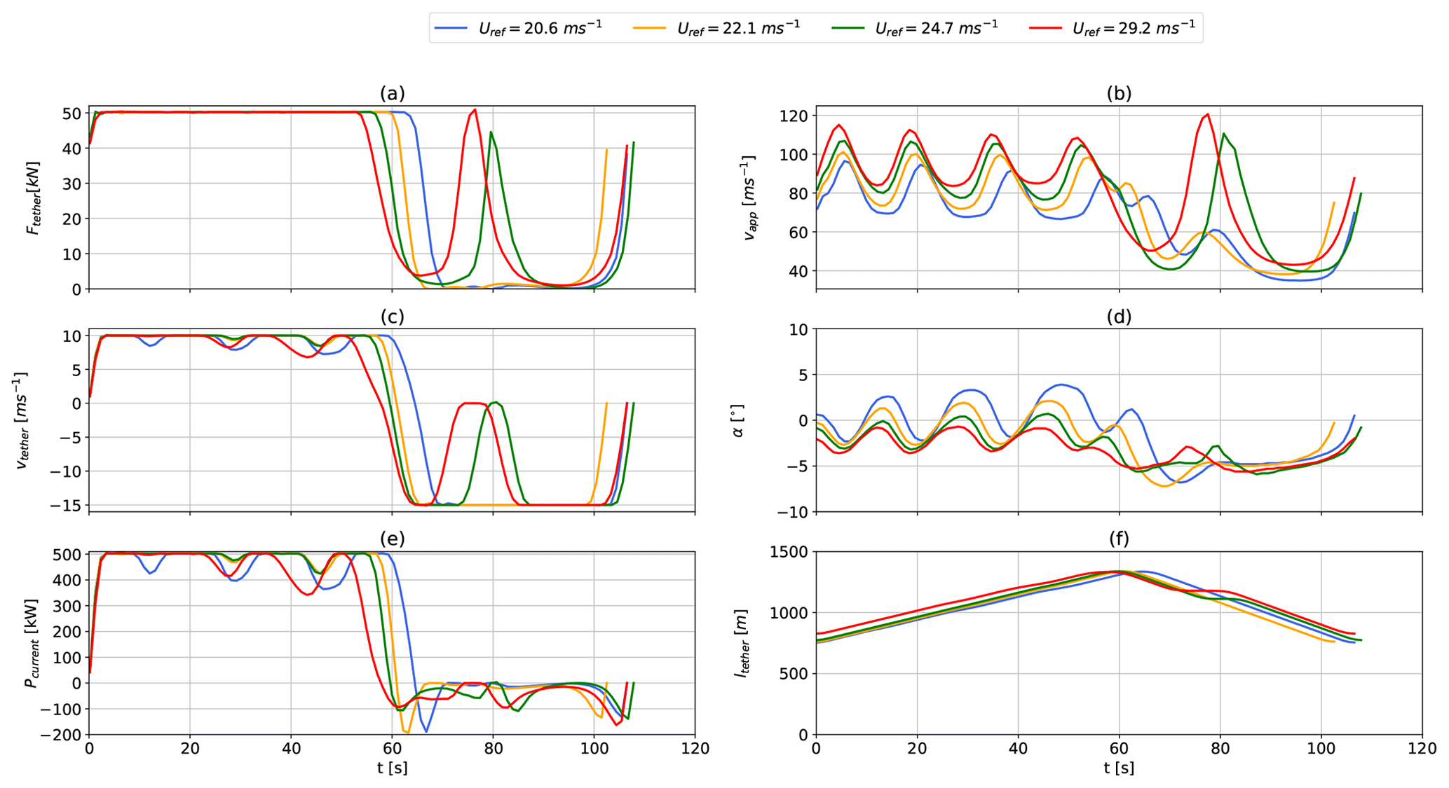
Figure A1Time series of instantaneous tether tension (a), apparent wind speed (b), tether-reeling speed (c), angle of attack (d), power output (e), and tether length (f) over one pumping based on high-wind-speed WRF-simulated offshore wind data. The results correspond to the trajectories shown in Fig. A2.
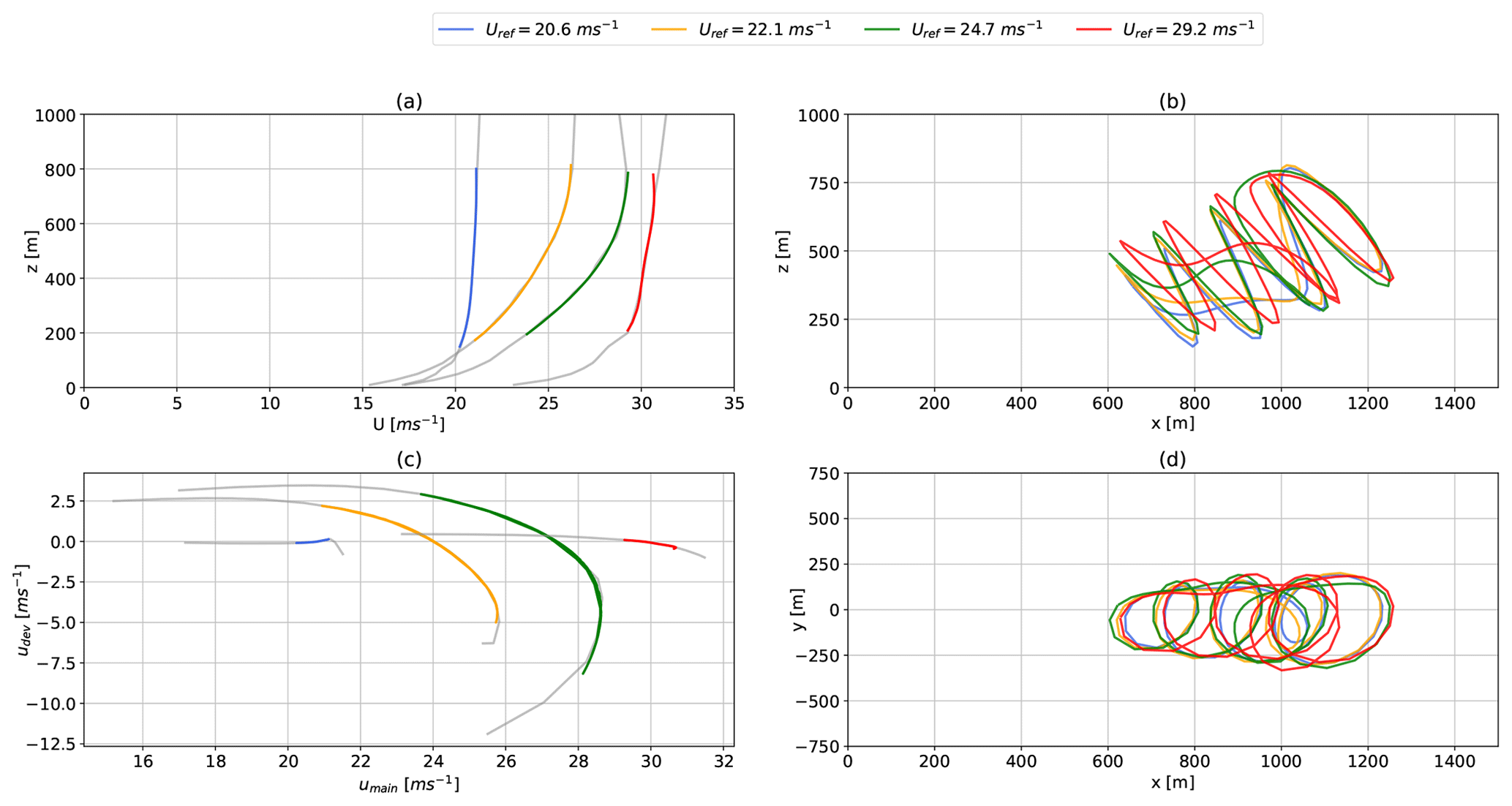
Figure A2High-wind-speed WRF-simulated vertical offshore wind speed profiles (a) and hodograph (top view) up to 1000 m (c). The highlighted sections indicate Lagrangian polynomial fit of the wind velocity at operating height. Panel (b) and panel (d) show the side and top view of the corresponding AWEBox-optimized trajectories. The reference wind speed in the legend is .
The results correspond to the time series shown in Fig. A1.
The simulated WRF data set can be accessed via https://doi.org/10.5281/zenodo.4292507 (Sommerfeld, 2020). It includes the 1 year of onshore and offshore horizontal wind speeds up to 1000 m, as well as the clusters implemented in this research. The format is a pickled .p Python dictionary.
MS evaluated the data and wrote the manuscript in consultation with and under the supervision of CC. MD set up the numerical offshore simulation and contributed to the meteorological evaluation of the data and reviewed the manuscript. JDS co-developed the optimization model and helped to write and review the manuscript.
The contact author has declared that none of the authors has any competing interests.
Publisher's note: Copernicus Publications remains neutral with regard to jurisdictional claims in published maps and institutional affiliations.
The authors thank the BMWi for the funding of the “OnKites I” and “OnKites II” projects (grant numbers 0325394 and 0325394A) on the basis of a decision by the German Bundestag and project management Projektträger Jülich. We thank the PICS, NSERC, and the DAAD for their funding.
AWEBox has been developed in collaboration with the company Kiteswarms Ltd. The company has also supported the AWEBox project through research funding. The AWEBox project has received funding from the European Union's Horizon 2020 research and innovation program under the Marie Skłodowska-Curie grant agreement no. 642682 (AWESCO).
We thank the Carl von Ossietzky University of Oldenburg and the Energy Meteorology research group for providing access to their high-performance computing cluster EDDY and ongoing support.
We further acknowledge Rachel Leuthold (University of Freiburg, SYSCOP) and Thilo Bronnenmeyer (Kiteswarms Ltd.) for their help in writing this article, great technical support, and continued work on the AWEBox toolbox.
This research has been supported by several sources. These include student scholarships from the Pacific Institute for Climate Solutions (PICS), the Natural Sciences and Engineering Research Council of Canada (NSERC), and the Deutscher Akademischer Austauschdienst (DAAD).
Additionally, projects and researchers whose contributions were essential to the writing of this article were funded by the European Union's Horizon 2020 research and innovation program under the Marie Skłodowska-Curie (grant agreement no. 642682), as well as the Bundesministerium für Wirtschaft und Energie (BMWi) (grant no 0324005, OnKites I grant no. 0325394, and OnKites II grant no. 0325394A).
This paper was edited by Roland Schmehl and reviewed by Mark Schelbergen, Maximilian Ranneberg, and one anonymous referee.
Abramowitz, M. and Stegun, I. A. (Eds.): Handbook of Mathematical Functions with Formulas, Graphs and Mathematical Tables, Dover Publications, Inc., New York, ISBN 0486612724, 1965. a, b
Airborne Wind Europe: Glossary – definitions of AWE-specific terms, https://airbornewindeurope.org/resources/glossary-2/ (last access: 29 March 2022), 2021. a, b, c, d
Ampyx Power BV: Ampyx Power is developing Airborne Wind Energy Systems, https://www.ampyxpower.com/ (last access: 26 April 2023), 2020. a, b, c, d, e
Archer, C. L., Colle, B. A., Veron, D. L., Veron, F., and Sienkiewicz, M. J.: On the predominance of unstable atmospheric conditions in the marine boundary layer offshore of the U.S. northeastern coast, J. Geophys. Res.-Atmos., 121, 8869–8885, https://doi.org/10.1002/2016JD024896, 2016. a
Argatov, I. and Silvennoinen, R.: Efficiency of Traction Power Conversion Based on Crosswind Motion, in: Airborne Wind Energy, edited by: Ahrens, U., Diehl, M., and Schmehl, R., Springer, Berlin, Heidelberg, 65–79, https://doi.org/10.1007/978-3-642-39965-7_4, 2013. a
Argatov, I., Rautakorpi, P., and Silvennoinen, R.: Estimation of the mechanical energy output of the kite wind generator, Renew. Energy, 34, 1525–1532, https://doi.org/10.1016/j.renene.2008.11.001, 2009. a
Arya, P. and Holton, J.: Introduction to Micrometeorology, International Geophysics, Elsevier Science, ISBN 9780120593545, 2001. a
European Wind Energy Association (EWEA): Wind energy-the facts: a guide to the technology, economics and future of wind power, Routledge, https://doi.org/10.4324/9781849773782, 2012. a
Aull, M., Stough, A., and Cohen, K.: Design Optimization and Sizing for Fly-Gen Airborne Wind Energy Systems, Automation, 1, 1–16, https://doi.org/10.3390/automation1010001, 2020. a
Banta, R. M.: Stable-boundary-layer regimes from the perspective of the low-level jet, Acta Geophys., 56, 58–87, https://doi.org/10.2478/s11600-007-0049-8, 2008. a
Bechtle, P., Schelbergen, M., Schmehl, R., Zillmann, U., and Watson, S.: Airborne wind energy resource analysis, Renew. Energy, 141, 1103–1116, https://doi.org/10.1016/j.renene.2019.03.118, 2019. a
Bronnenmeyer, T.: Optimal Control for Multi-Kite Emergency Trajectories, MS thesis, University of Stuttgart, Stuttgart, https://cdn.syscop.de/publications/Bronnenmeyer2018.pdf (last access: 9 November 2022), 2018. a
Carl von Ossietzky Universität Oldenburg: EDDY, https://www.uni-oldenburg.de/fk5/wr/hochleistungsrechnen/hpc-facilities/eddy/ (last access: 26 April 2023), 2018. a
Cherubini, A., Papini, A., Vertechy, R., and Fontana, M.: Airborne Wind Energy Systems: A review of the technologies, Renew. Sustain. Energ. Rev., 51, 1461–1476, https://doi.org/10.1016/j.rser.2015.07.053, 2015. a, b
Dee, D. P., Uppala, S. M., Simmons, A. J., Berrisford, P., Poli, P., Kobayashi, S., Andrae, U., Balmaseda, M. A., Balsamo, G., Bauer, P., Bechtold, P., Beljaars, A. C. M., van de Berg, L., Bidlot, J., Bormann, N., Delsol, C., Dragani, R., Fuentes, M., Geer, A. J., Haimberger, L., Healy, S. B., Hersbach, H., Hólm, E. V., Isaksen, L., Kållberg, P., Köhler, M., Matricardi, M., McNally, A. P., Monge-Sanz, B. M., Morcrette, J.-J., Park, B.-K., Peubey, C., de Rosnay, P., Tavolato, C., Thépaut, J.-N., and Vitart, F.: The ERA-Interim reanalysis: configuration and performance of the data assimilation system, Q. J. Roy. Meteorol. Soc., 137, 553–597, https://doi.org/10.1002/qj.828, 2011. a
De Schutter, J., Leuthold, R., Bronnenmeyer, T., Paelinck, R., and Diehl, M.: Optimal control of stacked multi-kite systems for utility-scale airborne wind energy, in: 2019 IEEE 58th Conference on Decision and Control (CDC), 11–13 December 2019, Nice, France, 4865–4870, https://doi.org/10.1109/CDC40024.2019.9030026, 2019. a, b, c
De Schutter, J., Malz, E., Leuthold, R., Bronnenmeyer, T., Paelinck,
R., and Diehl, M.: awebox: Modelling and optimal control of
single- and multiple-kite systems for airborne wind energy,
https://github.com/awebox/awebox (last access: 10 May 2023), 2020. a, b, c, d
Diehl, M.: Airborne Wind Energy: Basic Concepts and Physical Foundations, in: Airborne Wind Energy, edited by: Ahrens, U., Diehl, M., and Schmehl, R., Springer, Berlin, Heidelberg, 3–22, https://doi.org/10.1007/978-3-642-39965-7_1, 2013. a
Donlon, C. J., Martin, M., Stark, J., Roberts-Jones, J., Fiedler, E., and Wimmer, W.: The Operational Sea Surface Temperature and Sea Ice Analysis (OSTIA) system, Remote Sensing of Environment, 116, 140–158, https://doi.org/10.1016/j.rse.2010.10.017, 2012. a
Dörenkämper, M., Optis, M., Monahan, A., and Steinfeld, G.: On the Offshore advection of Boundary-Layer Structures and the Influence on Offshore Wind Conditions, Bound.-Lay. Meteorol., 155, 459–482, https://doi.org/10.1007/s10546-015-0008-x, 2015. a
Dörenkämper, M., Stoevesandt, B., and Heinemann, D.: Derivation of an offshore wind index for the German bight from high-resolution mesoscale simulation data, Proceedings of DEWEK – German Offshore Wind Energy Conference, p. 5, http://publica.fraunhofer.de/documents/N-484817.html (last access: 26 April 2023), 2017. a
Dörenkämper, M., Olsen, B. T., Witha, B., Hahmann, A. N., Davis, N. N., Barcons, J., Ezber, Y., García-Bustamante, E., González-Rouco, J. F., Navarro, J., Sastre-Marugán, M., Sīle, T., Trei, W., Žagar, M., Badger, J., Gottschall, J., Sanz Rodrigo, J., and Mann, J.: The Making of the New European Wind Atlas – Part 2: Production and evaluation, Geosci. Model Dev., 13, 5079–5102, https://doi.org/10.5194/gmd-13-5079-2020, 2020. a, b, c
Echeverri, P., Fricke, T., Homsy, G., and Tucker, N.: The Energy Kite – Selected Results From the Design, Development and Testing of Makani's Airborne Wind Turbines – Part 1, Technical Report, Makani Power, https://storage.googleapis.com/x-prod.appspot.com/files/Makani_TheEnergyKiteReport_Part1.pdf (last access: 9 November 2022), 2020. a
Eijkelhof, D. and Schmehl, R.: Six-degrees-of-freedom simulation model for future multi-megawatt airborne wind energy systems, Renew. Energy, 196, 137–150, https://doi.org/10.1016/j.renene.2022.06.094, 2022. a, b
Eijkelhof, D., Rapp, S., Fasel, U., Gaunaa, M., and Schmehl, R.: Reference Design and Simulation Framework of a Multi-Megawatt Airborne Wind Energy System, J. Phys.: Conf. Ser., 1618, 032020, https://doi.org/10.1088/1742-6596/1618/3/032020, 2020. a, b, c
Ellis, G. and Ferraro, G.: The Social Acceptance of Wind Energy: Where we stand and the path ahead, EUR – Scientific and Technical Research Reports, European Commission, https://doi.org/10.2789/696070, 2016. a
Emeis, S.: Wind energy meteorology: atmospheric physics for wind power generation, Green Energy and Technology, Springer, Berlin, Heidelberg, https://doi.org/10.1007/978-3-642-30523-8, 2013. a
EnerKíte GmbH: EnerKíte – Technologie, http://www.enerkite.de/ (last access: 10 May 2023), 2022. a
Faggiani, P. and Schmehl, R.: Design and Economics of a Pumping Kite Wind Park, in: Airborne Wind Energy: Advances in Technology Development and Research, edited by: Schmehl, R., Springer, Singapore, 391–411, https://doi.org/10.1007/978-981-10-1947-0_16, 2018. a, b
Fagiano, L. and Milanese, M.: Airborne Wind Energy: An overview, in: IEEE 2012 American Control Conference (ACC), 27–29 June 2012, Montreal, Canada, 3132–3143, https://doi.org/10.1109/ACC.2012.6314801, 2012. a
Fagiano, L., Quack, M., Bauer, F., Carnel, L., and Oland, E.: Autonomous Airborne Wind Energy Systems: Accomplishments and Challenges, Annu. Rev. Control Robot. Autonom. Syst., 5, 603–631, https://doi.org/10.1146/annurev-control-042820-124658, 2022. a
Fechner, U. and Schmehl, R.: Model-Based Efficiency Analysis of Wind Power Conversion by a Pumping Kite Power System, in: Airborne Wind Energy, Springer, Berlin, Heidelberg, 249–269, https://doi.org/10.1007/978-3-642-39965-7_14, 2013. a
Floors, R., Batchvarova, E., Gryning, S.-E., Hahmann, A. N., Peña, A., and Mikkelsen, T.: Atmospheric boundary layer wind profile at a flat coastal site – wind speed lidar measurements and mesoscale modeling results, Adv. Sci. Res., 6, 155–159, https://doi.org/10.5194/asr-6-155-2011, 2011. a, b, c
Gelaro, R., McCarty, W., Suárez, M. J., Todling, R., Molod, A., Takacs, L., Randles, C. A., Darmenov, A., Bosilovich, M. G., Reichle, R., Wargan, K., Coy, L., Cullather, R., Draper, C., Akella, S., Buchard, V., Conaty, A., da Silva, A. M., Gu, W., Kim, G.-K., Koster, R., Lucchesi, R., Merkova, D., Nielsen, J. E., Partyka, G., Pawson, S., Putman, W., Rienecker, M., Schubert, S. D., Sienkiewicz, M., and Zhao, B.: The Modern-Era Retrospective Analysis for Research and Applications, Version 2 (MERRA-2), J. Climate, 30, 5419–5454, https://doi.org/10.1175/JCLI-D-16-0758.1, 2017. a
Gros, S., Zanon, M., and Diehl, M.: A relaxation strategy for the optimization of airborne wind energy systems, in: IEEE, 2013 European Control Conference (ECC), 17–19 July 2013, Zurich, Switzerland, 1011–1016, https://doi.org/10.23919/ECC.2013.6669670, 2013. a
Haas, T., Schutter, J. D., Diehl, M., and Meyers, J.: Wake characteristics of pumping mode airborne wind energy systems, J. Phys.: Conf. Ser., 1256, 012016, https://doi.org/10.1088/1742-6596/1256/1/012016, 2019. a, b
Hahmann, A. N., Sīle, T., Witha, B., Davis, N. N., Dörenkämper, M., Ezber, Y., García-Bustamante, E., González-Rouco, J. F., Navarro, J., Olsen, B. T., and Söderberg, S.: The making of the New European Wind Atlas – Part 1: Model sensitivity, Geosci. Model Dev., 13, 5053–5078, https://doi.org/10.5194/gmd-13-5053-2020, 2020. a, b
Hartigan, J. A. and Wong, M. A.: Algorithm AS 136: A K-Means Clustering Algorithm, J. Roy. Stat. Soc. Ser. C, 28, 100–108, 1979. a
Heilmann, J. and Houle, C.: Economics of Pumping Kite Generators, in: Airborne Wind Energy, edited by: Ahrens, U., Diehl, M., and Schmehl, R., Springer, Berlin, Heidelberg, 271–284, https://doi.org/10.1007/978-3-642-39965-7_15, 2013. a
Hersbach, H. and Dick, D.: ERA5 reanalysis is in production, http://www.ecmwf.int/en/newsletter/147/news/era5-reanalysis-production (last access: 22 October 2019), 2016. a
Houska, B. and Diehl, M.: Optimal control for power generating kites, in: IEEE 2007 European Control Conference (ECC), 2–5 July 2007, Kos, Greece, 3560–3567, https://doi.org/10.23919/ECC.2007.7068861, 2007. a
HSL: HSL. A collection of Fortran codes for large scale scientific computation, http://www.hsl.rl.ac.uk/ (last access: 14 March 2022), 2020. a
Kruijff, M. and Ruiterkamp, R.: A Roadmap Towards Airborne Wind Energy in the Utility Sector, in: Airborne Wind Energy: Advances in Technology Development and Research, edited by: Schmehl, R., Springer, Singapore, 643–662, https://doi.org/10.1007/978-981-10-1947-0_26, 2018. a
Leuthold, R., De Schutter, J., Malz, E., Licitra, G., Gros, S., and Diehl, M.: Operational Regions of a Multi-Kite AWE System, in: 2018 European Control Conference (ECC), 12–15 June 2018, Limassol, Cyprus, 52–57, https://doi.org/10.23919/ECC.2018.8550199, 2018. a, b, c
Licitra, G.: Identification and optimization of an airborne wind energy system, PhD thesis, University of Freiburg, Freiburg, https://doi.org/10.6094/UNIFR/16226, 2018. a, b
Licitra, G., Koenemann, J., Bürger, A., Williams, P., Ruiterkamp, R., and Diehl, M.: Performance assessment of a rigid wing Airborne Wind Energy pumping system, Energy, 173, 569–585, https://doi.org/10.1016/j.energy.2019.02.064, 2019. a, b
Lloyd, S.: Least squares quantization in PCM, IEEE T. Inform. Theory, 28, 129–137, https://doi.org/10.1109/TIT.1982.1056489, 1982. a
Loyd, M. L.: Crosswind kite power (for large-scale wind power production), J. Energy, 4, 106–111, https://doi.org/10.2514/3.48021, 1980. a
Luchsinger, R. H.: Pumping Cycle Kite Power, in: Airborne Wind Energy, chap. 3, Green Energy and Technology, edited by: Ahrens, U., Diehl, M., and Schmehl, R., Springer, Berlin, Heidelberg, 47–64, https://doi.org/10.1007/978-3-642-39965-7_3, 2013. a, b
Lunney, E., Ban, M., Duic, N., and Foley, A.: A state-of-the-art review and feasibility analysis of high altitude wind power in Northern Ireland, Renew. Sustain. Energ. Rev., 68, 899–911, https://doi.org/10.1016/j.rser.2016.08.014, 2017. a, b
Malz, E., Koenemann, J., Sieberling, S., and Gros, S.: A reference model for airborne wind energy systems for optimization and control, Renew. Energy, 140, 1004–1011, https://doi.org/10.1016/j.renene.2019.03.111, 2019. a, b, c, d, e, f, g
Malz, E., Hedenus, F., Göransson, L., Verendel, V., and Gros, S.: Drag-mode airborne wind energy vs. wind turbines: An analysis of power production, variability and geography, Energy, 193, 116765, https://doi.org/10.1016/j.energy.2019.116765, 2020a. a
Malz, E., Verendel, V., and Gros, S.: Computing the power profiles for an Airborne Wind Energy system based on large-scale wind data, Renew. Energy, 162, 766–778, https://doi.org/10.1016/j.renene.2020.06.056, 2020b. a
Molina-García, A., Fernández-Guillamón, A., Gómez-Lázaro, E., Honrubia-Escribano, A., and Bueso, M. C.: Vertical Wind Profile Characterization and Identification of Patterns Based on a Shape Clustering Algorithm, IEEE Access, 7, 30890–30904, https://doi.org/10.1109/ACCESS.2019.2902242, 2019. a
Nakanishi, M. and Niino, H.: Development of an Improved Turbulence Closure Model for the Atmospheric Boundary Layer, J. Meteorol. Soc. Jpn. 87, 895–912, https://doi.org/10.2151/jmsj.87.895, 2009. a
Noth, A. and Siegwart, R.: Design of Solar Powered Airplanes for Continuous Flight, in: ETHZ lecture: “Aircraft and Spacecraft Systems: Design, Modeling and Control”, https://ethz.ch/content/dam/ethz/special-interest/mavt/robotics-n-intelligent-systems/asl-dam/documents/projects/Design_Skysailor.pdf (last access: 5 July 2023), 2006. a
Obukhov, A. M.: Turbulence in an atmosphere with a non-uniform temperature, Bound.-Lay. Meteorol., 2, 7–29, https://doi.org/10.1007/BF00718085, 1971. a, b
offshorewind.biz: Ampyx Power Taking First Steps Towards MW-Scale Kite, https://www.offshorewind.biz/2018/12/04/ampyx-power-taking-first-steps-towards-mw-scale-kite/ (last access: 14 March 2022), 2018. a
Olauson, J.: ERA5: The new champion of wind power modelling?, Renew. Energy, 126, 322–331, https://doi.org/10.1016/j.renene.2018.03.056, 2018. a
Pedregosa, F., Varoquaux, G., Gramfort, A., Michel, V., Thirion, B., Grisel, O., Blondel, M., Prettenhofer, P., Weiss, R., Dubourg, V., Vanderplas, J., Passos, A., Cournapeau, D., Brucher, M., Perrot, M., and Duchesnay, E.: Scikit-learn: Machine Learning in Python, J. Mach. Learn. Res., 12, 2825–2830, https://doi.org/10.48550/arXiv.1201.0490, 2011. a, b, c
Peña, A., Gryning, S.-E., and Floors, R.: Lidar observations of marine boundary-layer winds and heights: a preliminary study, Meteorol. Z., 24, 581–589, https://doi.org/10.1127/metz/2015/0636, 2015. a
Powers, J., Ahmadov, R., Barlage, M., Carson, L., Chen, M., Dudhia, J., Fast, J., FitzGerald, K., Gaudet, B., Gill, D., Liu, J., Wang, W., and Werner, K.: WRF Source Codes and Graphics Software Download Page, https://www2.mmm.ucar.edu/wrf/users/download/get_source.html (last access: 9 May 2023), 2023. a
Ranneberg, M., Wölfle, D., Bormann, A., Rohde, P., Breipohl, F., and Bastigkeit, I.: Fast Power Curve and Yield Estimation of Pumping Airborne Wind Energy Systems, in: Airborne Wind Energy: Advances in Technology Development and Research, edited by: Schmehl, R., Springer, Singapore, 623–641, https://doi.org/10.1007/978-981-10-1947-0_25, 2018. a, b
Salvação, N. and Guedes Soares, C.: Wind resource assessment offshore the Atlantic Iberian coast with the WRF model, Energy, 145, 276–287, https://doi.org/10.1016/j.energy.2017.12.101, 2018. a
Schelbergen, M., Kalverla, P. C., Schmehl, R., and Watson, S. J.: Clustering wind profile shapes to estimate airborne wind energy production, Wind Energ. Sci., 5, 1097–1120, https://doi.org/10.5194/wes-5-1097-2020, 2020. a, b, c, d
Schmehl, R., Noom, M., and van der Vlugt, R.: Traction Power Generation with Tethered Wings, in: Airborne Wind Energy, chap. 2, edited by: Ahrens, U., Diehl, M., and Schmehl, R., Springer, Berlin, Heidelberg, 23–45, https://doi.org/10.1007/978-3-642-39965-7_2, 2013. a, b, c
Sempreviva, A. M. and Gryning, S.-E.: Humidity fluctuations in the marine boundary layer measured at a coastal site with an infrared humidity sensor, Bound.-Lay. Meteorol., 77, 331–352, https://doi.org/10.1007/BF00123531, 1996. a, b
Skamarock, W., Klemp, J., Dudhia, J., Gill, D., Barker, D., Duda, M., Huang, X., Wang, W., and Powers, J.: A description of the advanced research WRF version 3, Tech. Rep. NCAR/TN−475+STR, NCAR – National Center for Atmospheric Research, Boulder, Colorado, USA, https://doi.org/10.5065/D68S4MVH, 2008. a, b
Skamarock, W. C., Klemp, J. B., Dudhia, J., and Gill, D. O.: A Description of the Advanced Research WRF Model Version 4.3, Technical Report, UCAR, https://doi.org/10.5065/1dfh-6p97, 2021. a, b
Sommerfeld, M.: Onshore & offshore WRF generated wind data, Zenodo [data], version 1, https://doi.org/10.5281/zenodo.4292507, 2020 a
Sommerfeld, M., Crawford, C., Monahan, A., and Bastigkeit, I.: LiDAR-based characterization of mid-altitude wind conditions for airborne wind energy systems, Wind Energy, 22, 1101–1120, https://doi.org/10.1002/we.2343, 2019a. a, b, c, d, e, f
Sommerfeld, M., Dörenkämper, M., Steinfeld, G., and Crawford, C.: Improving mesoscale wind speed forecasts using lidar-based observation nudging for airborne wind energy systems, Wind Energ. Sci., 4, 563–580, https://doi.org/10.5194/wes-4-563-2019, 2019b. a, b, c, d, e, f, g
Sommerfeld, M., Dörenk¨amper, M., De Schutter, J., and Crawford, C.: Scaling effects of fixed-wing ground-generation airborne wind energy systems, Wind Ener. Sci., 7, 1847–1868, https://doi.org/10.5194/wes-7-1847-2022, 2022. a, b, c
Stull, R.: An Introduction to Boundary Layer Meteorology, in: Atmospheric and Oceanographic Sciences Library, Springer Netherlands, https://doi.org/10.1007/978-94-009-3027-8, 1988. a
Terink, E. J., Breukels, J., Schmehl, R., and Ockels, W. J.: Flight Dynamics and Stability of a Tethered Inflatable Kiteplane, J. Aircraft, 48, 503–513, https://doi.org/10.2514/1.C031108, 2011. a
Vander Lind, D.: Analysis and Flight Test Validation of High Performance AirborneWind Turbines, in: Airborne Wind Energy, edited by: Ahrens, U., Diehl, M., and Schmehl, R., Springer, Berlin, Heidelberg, 473–490, https://doi.org/10.1007/978-3-642-39965-7_28, 2013. a
van der Vlugt, R., Peschel, J., and Schmehl, R.: Design and Experimental Characterization of a Pumping Kite Power System, in: Airborne Wind Energy, edited by: Ahrens, U., Diehl, M., and Schmehl, R., Springer, Berlin, Heidelberg, 403–425, https://doi.org/10.1007/978-3-642-39965-7_23, 2013. a, b
van der Vlugt, R., Bley, A., Noom, M., and Schmehl, R.: Quasi-steady model of a pumping kite power system, Renew. Energy, 131, 83–99, https://doi.org/10.1016/j.renene.2018.07.023, 2019. a, b, c, d, e
van Hagen, L., Petrick, K., Wilhelm, S., and Schmehl, R.: Life-Cycle Assessment of a Multi-Megawatt Airborne Wind Energy System, Energies, 16, 1750, https://doi.org/10.3390/en16041750, 2023. a, b
Van Sark, W. G., Van der Velde, H. C., Coelingh, J. P., and Bierbooms, W. A.: Do we really need rotor equivalent wind speed?, Wind Energy, 22, 745–763, https://doi.org/10.1002/we.2319, 2019. a
Vermillion, C., Cobb, M., Fagiano, L., Leuthold, R., Diehl, M., Smith, R. S., Wood, T. A., Rapp, S., Schmehl, R., Olinger, D., and Demetriou, M.: Electricity in the air: Insights from two decades of advanced control research and experimental flight testing of airborne wind energy systems, Annu. Rev. Control, 52, 330–357, https://doi.org/10.1016/j.arcontrol.2021.03.002, 2021. a
Waechter, A. and Laird, C.: Ipopt (Interior Point OPTimizer), https://github.com/coin-or/Ipopt (last access: 14 March 2022), 2016. a
Wharton, S. and Lundquist, J. K.: Atmospheric stability affects wind turbine power collection, Environ. Res. Lett., 7, 014005, https://doi.org/10.1088/1748-9326/7/1/014005, 2012. a
Witha, B., Hahmann, A., Sile, T., Dörenkämper, M., Ezber, Y., Bustamante, E., Gonzalez-Rouco, J., Leroy, G., and Navarro, J.: Report on WRF model sensitivity studies and specifications for the mesoscale wind atlas production runs: Deliverable D4.3, vol. D4.3, NEWA – New European Wind Atlas, Zenodo, https://doi.org/10.5281/zenodo.2682604, 2019. a