the Creative Commons Attribution 4.0 License.
the Creative Commons Attribution 4.0 License.
 | 16 Aug 2023
Lessons learned in coupling atmospheric models across scales for onshore and offshore wind energy
Branko Kosović
Larry K. Berg
Colleen M. Kaul
Matthew Churchfield
Jeffrey Mirocha
Dries Allaerts
Thomas Brummet
Shannon Davis
Amy DeCastro
Susan Dettling
Caroline Draxl
David John Gagne
Patrick Hawbecker
Pankaj Jha
Timothy Juliano
William Lassman
Eliot Quon
Raj K. Rai
Michael Robinson
William Shaw
Regis Thedin
The Mesoscale to Microscale Coupling team, part of the U.S. Department of Energy Atmosphere to Electrons (A2e) initiative, has studied various important challenges related to coupling mesoscale models to microscale models for the use case of wind energy development and operation. Several coupling methods and techniques for generating turbulence at the microscale that is subgrid to the mesoscale have been evaluated for a variety of cases. Case studies included flat-terrain, complex-terrain, and offshore environments. Methods were developed to bridge the terra incognita, which scales from about 100 m through the depth of the boundary layer. The team used wind-relevant metrics and archived code, case information, and assessment tools and is making those widely available. Lessons learned and discerned best practices are described in the context of the cases studied for the purpose of enabling further deployment of wind energy.
- Article
(5369 KB) - Full-text XML
- BibTeX
- EndNote


Whether one is planning for where to deploy future wind farms, micrositing turbines within a wind farm, or designing optimal wind farm control, it is crucial to include the impacts of the large-scale (mesoscale, meaning thousands to hundreds of thousands of meters) flow as well as to model at the microscale (on the order of meters to tens of meters). As much of the energy of the atmosphere resides in the largest scales, correctly modeling those scales as well as the turbulence and energy dissipation at the microscale provides the most accurate picture of the flow and energy available for harvest.
The models for the two scales tend to be disparate, however. Although both sets of models are numerical discretizations of the Navier–Stokes equations, they are built for different purposes. The mesoscale models are formulated for weather forecasting; have larger grid spacing over larger domains; and include parameterizations of many of the processes that are important for correctly modeling atmospheric flow, such as radiative transfer (shortwave incoming and longwave outgoing), boundary layers, surface layers, cloud microphysics, land surface models, and more. Including such parameterizations is necessary to predict the flow accurately. Mesoscale models are also initialized with initial and boundary conditions from global models, which include the day-to-day weather fluctuations. On the other hand, microscale models are able to resolve details of terrain and wind turbines at a scale not available to the mesoscale models. But the microscale models do not include all of the atmospheric-physics parameterizations of the mesoscale models. Thus, the solution to obtaining accurate flow prediction representing all relevant scales is to couple the mesoscale models to the microscale model.
Such coupling has long been a goal of modelers, but there have been a myriad of issues to work out. Some issues include the following:
-
The mesoscale models are usually fully compressible, while microscale models are typically incompressible or Boussinesq, where density differences are ignored except as they change buoyancy.
-
The gap between the typical resolutions of the two types of models – between about 100 m and traditionally 1000 m – known as the inner “grey zone” or the terra incognita, has been difficult to bridge (Wyngaard, 2004) (see Sect. 2.1).
-
Treatment of surface conditions is often inherently different due to surface inhomogeneities that become important at the microscale (see Sect. 2.2).
-
The best ways to couple the two models must be identified (see Sect. 2.3).
-
One must find ways to initiate turbulence at the microscale that is not resolved at the mesoscale (see Sect. 2.4).
-
Adding complexity, whether it comes from complex terrain or coupling atmosphere to ocean and wave models, complicates the picture and requires separate treatment (see Sect. 2.6).
-
Assessing how the models perform must be accomplished in the context of wind energy needs (see Sect. 2.7).
-
The uncertainty in the model results should be quantified to be most useful (see Sect. 2.5).
-
There is room for improvement in model parameterization (see Sect. 4.1 and 4.2).
-
And finally, how can modern techniques such as improved parameterizations and machine learning be leveraged to improve modeling (see Sect. 4.2 and 4.3)?
As part of the U.S. Department of Energy (DOE) Atmosphere to Electrons (A2e) initiative, the Mesoscale to Microscale Coupling (MMC) team was charged with studying these issues and more. The goal of the project has been to improve coupling between mesoscale and microscale simulations via enhanced guidance and create new strategies for setting up simulations and for the development of new tools that can be used across the community. This philosophy recognizes that including the mesoscale forcing is critical to modeling the full energy transfer across scales in the atmosphere. Specific objectives include the following:
-
apply verification and validation techniques to the new modeling tools and develop estimates of the uncertainty,
-
reduce turbulence spin-up time in microscale simulations and hence decrease their computational cost,
-
improve the surface-layer treatment in microscale models to more accurately simulate wind speed and shear over the rotor diameter,
-
develop best-practice guidance for the community,
-
prepare and document a suite of software tools that can be used across the community, and
-
transition MMC research to the offshore environment.
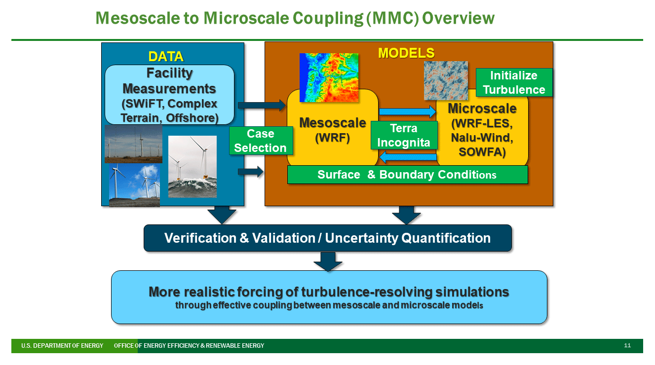
Figure 1The MMC team's case-based approach to addressing challenges of coupling the mesoscale to the microscale. Flat-terrain image from the DOE Scaled Wind Farm Facility site at https://www.depts.ttu.edu/nwi/research/facilities/swift.php (last access: 23 July 2023). Complex-terrain figure taken by Sue Ellen Haupt. Offshore-wind figure from the DOE Wind Energy Technologies Office at https://www.energy.gov/eere/wind/wind-energy-technologies-office (last access: 23 July 2023). Mesoscale example thanks to Raj Rai and microscale image by Matthew Churchfield.
Figure 1 illustrates the team's approach. The goal is to provide more realistic turbulence-resolving simulations through coupling these scales. The team leveraged a case study approach to address these issues (Haupt et al., 2019a). By working in the framework of studying particular situations for which we have observations, we can better develop and assess tools to best match real-world situations, which is particularly important for studying nonstationary meteorological conditions (such as frontal passages, thunderstorm outflows, baroclinic systems, and low-level jets) or when considering changes in atmospheric stability associated with the diurnal cycle. In essence, the objective is to have the microscale model “follow” the mesoscale model through dynamic changes while appropriately modeling the fine-scale behavior of the flow. The approach is to select case studies from field programs or observational data to identify challenging atmospheric conditions and test methods to simulate them. Most of these datasets are from DOE-sponsored facilities in flat and complex terrain as well as from offshore sites and are available on the Wind Data Hub (Atmosphere to Electrons, 2023). The mesoscale modeling has focused on a widely used community model, the Weather Research and Forecasting (WRF) model (Skamarock et al., 2008). Several microscale models have been tested, including the large-eddy simulation (LES) version of WRF (WRF-LES) that can be run online, where the inner nest derives the conditions directly from the outer nest during the simulation, and several offline models, such as Nalu-Wind (Kaul et al., 2020) and the Simulator fOr Wind Farm Applications (SOWFA; Churchfield et al., 2012), which are run after the mesoscale model with inputs derived from those previous runs. Some aspects of the coupling that merit study include the surface and boundary conditions; bridging the terra incognita; initializing turbulence at the microscale that is not resolved at the mesoscale; the coupling methods themselves; and dealing with multiple sources of flow complexity, including complex terrain, coastal flows, and offshore flows. The testing is grounded in rigorous verification and validation configured specifically for wind energy plus uncertainty quantification, emphasizing determining parametric uncertainty in turbulence modeling in microscale simulations.
An emphasis of the project is testing, evaluating, and comparing multiple methods of coupling the outer mesoscale flow to the microscale flow. Some methods use a single model (currently, WRF) at both scales, which ensures continuity across scales (internal coupling). Other methods incorporate forcing information from the mesoscale into a stand-alone microscale model (external coupling). This work is based on several preliminary investigations using WRF for both internal (Liu et al., 2011; Mirocha et al., 2014b; Muñoz-Esparza et al., 2014, 2015) and external (Zajaczkowski et al., 2011; Gopalan et al., 2014) MMC, showing both promise and direction for future development. Rigorous comparisons of methods for different conditions and use cases provide insight into best practices. Another effort seeks to compare different methods of generating turbulence in the microscale models that is unresolved by the mesoscale forcing. The turbulence generation intercomparison was greatly facilitated by the development of Python-based assessment tools that are used via shared Jupyter Notebooks. This effort includes design, testing, and deploying common code bases to simulate and assess the flows, which are now available on the public MMC GitHub (Quon et al., 2023a).
The team has archived simulation codes and model workflows for a range of case studies that can be used as a starting point for users to develop their own applications. Model codes and preprocessing and postprocessing scripts are available on GitHub in Quon et al. (2023a, b, c), Gill et al. (2023), and Hawbecker et al. (2023a). Online documentation resides in a “Read the Docs” format (Mesoscale-to-Microscale Coupling, 2023). The goal of the code and workflow release is to promote high-fidelity coupled simulation capability to advance wind energy deployment through better knowledge of the atmospheric conditions that drive energy harvest in wind farms. Modelers are invited to test our models and workflows available in the GitHub references listed above.
This paper describes what we have learned about some of the difficult issues of coupling (Sect. 2); presents case studies that were accomplished (Sect. 3); and discusses how enhanced methods, such as improved parameterizations and machine learning, can help accomplish our goals (Sect. 4). Section 5 concludes with a summary and a list of lessons learned plus suggests where future research should focus. Recommendations for best practices are sprinkled throughout the paper.
The course of the research has investigated the topics laid out in Sect. 1, and here we summarize the work that has led to lessons we have learned.
2.1 The terra incognita
In coupled mesoscale–microscale simulations, including horizontal grid resolutions falling within the terra incognita is almost inevitable. The terra incognita, coined by Wyngaard (2004), is the range of horizontal grid spacings where turbulence models used in both mesoscale and LESs do not work properly. The MMC project investigated the impact of the terra incognita in coupled simulations (Rai et al., 2017, 2019). Our work suggests that the impact of the terra incognita can be minimized using an appropriate choice of the horizontal grid spacing, turbulence modeling (dependent on the horizontal grid spacing), and grid refinement ratio (GRR) applied between the mesoscale and microscale simulations. The most important consideration is that the horizontal grid spacing of the mesoscale simulation should be at least comparable to the boundary layer depth. Horizontal grid spacing smaller than the boundary layer depth produces erroneous structures in the simulated flow. Applying a GRR that allows for simulations to jump over the terra incognita not only alleviates the problem but also reduces the number of computational domains. A larger value of GRR, however, also increases the fetch needed to generate turbulence on nested domains due to the inertia of larger structures transported from the parent domain. The need for a larger fetch can be mitigated by applying perturbations along the inflow boundaries of the domain (Sect. 2.4). In situations when the GRR (between mesoscale and microscale domains) becomes large, it can be beneficial to use the LES three-dimensional (3D) turbulence model (e.g., Smagorinsky, 1963) in the terra incognita region, provided that the horizontal grid spacing is closer to 100 m, and then jump to grid spacing larger than the boundary layer depth using the GRR (Rai et al., 2019). However, the use of a 3D LES closure when the grid spacing is too coarse to resolve any of the motions responsible for momentum transport can result in incorrect stress profiles, leading to significant errors in wind speed within the atmospheric boundary layer (ABL). The recently developed 3D planetary boundary layer (PBL) Mellor–Yamada scheme (Juliano et al., 2022) fills a critical gap in this regard, providing for a consistent representation of transport at scales finer than traditional mesoscale applications but at scales too coarse to rely upon a 3D LES turbulence closure (Sect. 4.1).
2.2 Surface layer
The surface layer (SL) traditionally represents approximately the lowest 10 % of the atmospheric boundary layer (ABL), within which the vertical fluxes of heat, momentum, and other constituents are assumed to approach nearly constant distributions with height above the surface. Parameterization of the exchanges of these quantities between the surface and the atmosphere within atmospheric models relies upon various SL scaling relationships, since the vertical grid spacing in such models is generally too coarse to use a no-slip boundary condition. The particular SL scaling employed, along with characteristics of the model spatial discretization and the turbulence closure employed to model turbulent exchanges above the surface, all interact to influence the application of the surface boundary condition in atmospheric models and subsequently impact resulting flow and other SL and ABL characteristics.
The most commonly employed SL scaling relationship used within atmospheric models is the Monin–Obukhov similarity theory (MOST; Monin and Obukhov, 1954). MOST provides relationships to parameterize the fluxes between the surface and atmosphere based on a small number of surface and near-surface atmospheric-flow parameters. While MOST is well established, relatively simple, and widely used, it is based on a number of assumptions, including uniform terrain, horizontal homogeneity of both surface and atmospheric variables of interest, steady flow and forcing conditions over time, and the appropriateness of ensemble mean values of the parameterized fluxes. These assumptions are reasonably well satisfied in most historical numerical weather prediction and mesoscale atmospheric simulations, due in part to the use of coarse grid spacing, which satisfies the appropriateness of ensemble mean representations within each grid cell, while also not resolving sharp transitions in terrain features, horizontal heterogeneities, and meteorological forcing. However, the recent transition toward the use of higher resolution in many mesoscale applications sharpens the representation of some or all of these features, all of which increasingly violate the assumptions upon which MOST is based.
While the use of high horizontal resolution violates the applicability of MOST for one set of reasons, the use of high vertical resolution can create additional problems, especially in settings for which a logarithmic mean profile shape is not expected, such as within forest canopies or over significant surface waves or ocean swell. Moreover, care must be taken not to place the lowest model grid cell too close to the surface.
Microscale atmospheric LES models also routinely apply MOST to formulate the surface stresses at each surface grid cell based on the instantaneous time-varying horizontal velocities above. Even under highly idealized conditions satisfying the assumptions of MOST in the aggregate, such models violate the appropriateness of the ensemble mean assumption.
Despite the abovementioned caveats, MOST is still routinely applied in atmospheric simulations at all scales, owing primarily to a dearth of alternatives. To improve its applicability, as well as the performance of simulating flow within the SL more generally, numerous approaches have been developed, including various damping (Mason and Thomson, 1992) and correction factors (Khani and Porté-Agel, 2017), the use of more advanced turbulence subgrid-scale (SGS) models (Bou-Zeid et al., 2005; Chow et al., 2004), taking care to properly set the computational mesh to have the proper width-to-height ratio (Brasseur and Wei, 2010), and the use of additional near-wall stress parameterizations (Brown et al., 2001) to distribute the surface stresses vertically. The impacts of many of these methods on improving LES performance within the WRF model in wind-energy-relevant applications has been examined in Mirocha et al. (2010), Kirkil et al. (2012), Mirocha et al. (2013), and Mirocha et al. (2014b).
SL modeling has also been extended to applications over forested landscapes for which a logarithmic vertical profile of mean wind speed is not observed (see review by Patton and Finnigan, 2012). These methods are based on the addition of momentum sink terms to the governing horizontal momentum equations to account for the increased drag effects of foliage, with the magnitude of the drag expressed in terms of a leaf area index, which represents the surface area of vegetation as a function of height. Modifications to elements of the SGS model, including eddy viscosity coefficients and SGS turbulence kinetic energy (TKE), may also be included in such formulations.
Arthur et al. (2019) implemented the plant canopy model of Shaw and Patton (2003) into the WRF model and demonstrated the ability of WRF-LES to recover expected distributions of winds and turbulence quantities in an idealized plant canopy. Arthur et al. (2019) additionally combined concepts from the plant canopy approach and the near-wall stress models used in various LES SGS formulations (Kirkil et al., 2012) to develop a novel distributed drag implementation for the parameterized surface stresses. This model applies the expected surface momentum stresses as drag terms in the horizontal momentum equations, distributed vertically over the several lowest model grid cells. When applied in LESs using the MOST surface boundary condition, this approach significantly improves agreement between simulated mean wind speed profiles and their expected similarity relationships.
In addition to improving the implementation of MOST within atmospheric solvers, significant progress has also been achieved in developing an alternative to MOST using machine learning (ML) to relate surface exchange to relevant atmospheric and surface parameters obtained from observations. Details of this approach are provided in Sect. 4.2.
2.3 Coupling methods
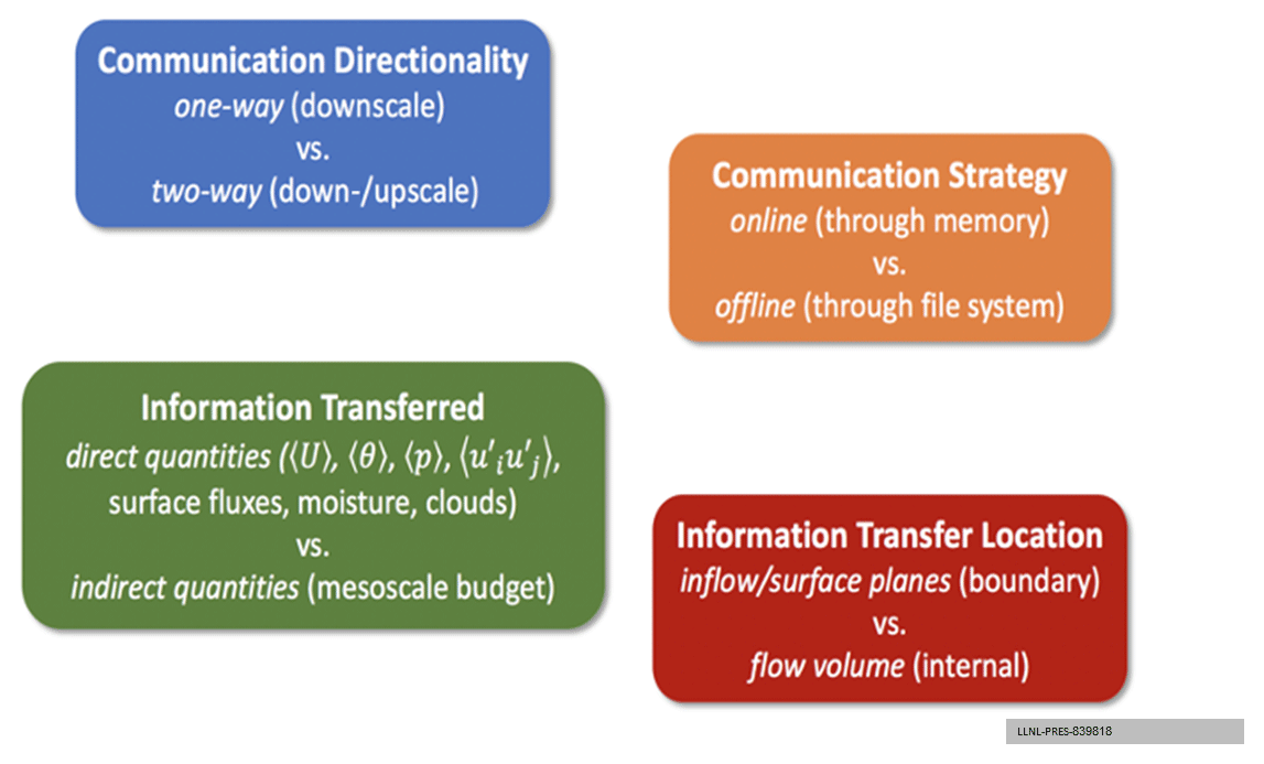
Over the course of this project, we have explored different frameworks for coupling mesoscale simulations to microscale LESs. Figure 2 depicts the various ways of classifying coupling strategies. Coupling approaches can be classified according to the following properties: communication directionality (i.e., one-way or two-way coupling), communication strategy (i.e., online through system memory or offline through file system), information transferred (i.e., direct quantities such as wind speed, temperature, and surface fluxes or indirect quantities such as tendencies from the mesoscale budget), and the information transfer location (i.e., inflow/surface planes at the LES boundary or through the entire flow volume). A comparatively low-cost method for coupling the mesoscale to the microscale is via an offline, periodic LES, which includes internal height–time-varying source terms that provide mesoscale influence on the microscale. For this approach, mesoscale simulation output is saved over a one-dimensional (1D) column at a regular temporal interval (e.g., 10 min); this information is used with data assimilation techniques to force the periodic simulation toward the desired mesoscale behavior. One way to achieve this forcing is through what we term “profile assimilation”, in which the microscale velocity and potential temperature solutions are plane-averaged at each height at a given time. Those resultant mean profiles are compared with the desired mesoscale profiles, and the difference is used to determine the amount of forcing required to drive the microscale mean vertical profiles to match those of the mesoscale. One of the key lessons learned in this study is that with a strong forcing that enforces the microscale mean vertical profiles to very closely match those of the mesoscale (what we term “direct profile assimilation”), unrealistic turbulent fields sometimes form in the microscale simulation. This may be a natural LES response to mesoscale profiles that are superadiabatic over too much of their vertical extent. To deal with this, we developed a method that allows the microscale simulation more freedom to depart from the exact mesoscale vertical structure (what we term “indirect profile assimilation”) but which will follow all the mesoscale trends in time (Allaerts et al., 2020, 2023). Alternatively, the mesoscale forcing can be included by imposing height–time-varying source terms in the microscale LES. The forcing accounts for large-scale advection and the driving pressure gradient and is extracted from the mesoscale simulation (Draxl et al., 2021). Any of these methods, though, assume a horizontally homogeneous forcing field and are applicable only to homogeneous cases that are well represented by periodic boundary conditions. Although it is theoretically possible to apply an internal source term that varies three-dimensionally in space to represent horizontally heterogeneous situations, we have not explored that approach; however, others (Sanz-Rodrigo et al., 2021) have demonstrated the validity of that approach. Instead, for horizontally heterogeneous domains or simulations that resolve turbines, we have focused our attention on boundary-coupled simulations, which provide the highest degree of generality. Boundary-coupled simulations can be conducted via online or offline coupling.
For offline coupling, the mesoscale output once again needs to be saved at regular temporal intervals to provide boundary forcing for the LES. However, instead of 1D profiles, two-dimensional (2D) planes must be saved, which increases the input/output (I/O) and storage requirements considerably. Boundary coupling allows for simulation of a heterogeneous domain for resolving complex terrain, mesoscale flows with significant horizontal gradients, or wind farms.
Online-coupled cases downscale from the mesoscale through nesting, usually within a single code; this allows for a potentially streamlined workflow, as the downscaling usually involves setting runtime input parameters. Advantages of an online-coupled simulation is the ability to use consistent numerics and complete atmospheric physics across spatial scales, as well as the ability to perform two-way coupling. However, because mesoscale meteorology models are usually not developed with LES applications in mind, this coupling approach requires greater overhead and poorly optimized parallelization of computing resources for the LES domain, imposing severe restrictions on the ability to conduct large numbers of simulations. Note that a current DOE initiative focuses on development of mesoscale (ERF, Energy Research and Forecasting model) and microscale (AMR-Wind; adaptive mesh refinement) models that are aimed at exascale high-performance computing (HPC) platforms. However, also note that online coupling of mesoscale and microscale models that are based on the same formulation, i.e., equations, and use the same numerical discretization simplifies coupling and results in more consistent simulations across scales. Offline boundary-coupled simulations, however, are able to achieve higher simulation throughput, which is crucial for parameter selection, sensitivity studies, or wind plant design applications. We conducted a series of case studies directly comparing these approaches: one in a flat, fairly homogeneous onshore environment (Sect. 3.1, Allaerts et al., 2020; Draxl et al., 2021; Allaerts et al., 2023) and one in the offshore environment (Sect. 3.5, Thedin et al., 2023). Further case studies demonstrate the use of these techniques in complex terrain (Sect. 3.3 and 3.4), resolving the coastal boundary (Sect. 3.6), or in the offshore environment with variable shallow-water roughness and sea surface temperature (Sect. 3.6).
We note that while the stand-alone microscale solver adds complexity to the setup, it allows for greater flexibility. Most importantly, it allows for the study of the interaction of realistic weather conditions, complex terrain, and turbines. The turbines can be coupled with aero-servo-elastic models using OpenFAST (2022; see Sect. 3.5.2). In the workflows presented in this paper, the turbine can be represented by actuator disk or actuator line models. Note that the stand-alone, offline approach even allows for the use of blade-resolved approaches.
2.4 Initializing turbulence
LESs are designed to explicitly resolve the energetically important scales of turbulence and the resulting fluxes and transport those motions generate within the flow. Models using grid spacings that are too coarse to resolve those motions must instead rely on parameterizations (e.g., PBL schemes) to represent those processes. Therefore, when forcing LESs with mesoscale atmospheric data at the domain boundaries, either online or offline, a domain fetch is required for the resolved scales of motion to appear within the LES flow field, since those motions are not resolved within the inflow data. A similar issue is encountered when forcing LESs with observations, as most observational datasets do not contain sufficient spatiotemporal frequency to specify the turbulence field. In each of these cases, the fetch required for resolved-scale turbulence motions to form and equilibrate to the large-scale forcing within the LES domain can be extensive and represents a significant computational burden. The amount of fetch required depends on multiple contributing factors, including surface roughness and terrain, wind speed, and atmospheric stability. Generally, for a computation using specified inflow conditions during unstable conditions, the reduction in fetch due to perturbations can be small, perhaps only around 100 grid cells in the direction of the mean flow. However, during neutral or stable conditions, perturbation can foreshorten the fetch by several hundred grid points, which can constitute a computational savings of 50 % or more. Moreover, the flow field within the fetch will not represent either the mean or turbulence fields during the process of turbulence spin-up and equilibration well.1 To ameliorate both the computational overhead and flow inaccuracies within LESs forced in this manner, several inflow perturbation methods have been developed and examined within the MMC project. These methods have been shown to successfully promote the formation and equilibration of resolved-scale turbulence within LESs driven by mesoscale data and low-frequency observations, leading to substantial reductions in computational expense by permitting the use of smaller LES domains while simultaneously improving the accuracy of the flow field beyond the fetch. The inflow turbulence perturbation approaches that were examined within the project are briefly described below.
2.4.1 Stochastic cell perturbation method
The cell perturbation method (CPM) is based on the application of perturbed values of atmospheric temperature or velocity to “cells” (groups of contiguous model grid points in the horizontal and vertical directions) located just within the lateral edges of an LES domain (Muñoz-Esparza et al., 2014, 2015; Mazzaro et al., 2019). Optimal choices for the amplitude, size, and number of cells impart variability upon the inflow that rapidly generates resolved-scale turbulence. Since the magnitude of the perturbation applied within each cell is drawn from a random distribution with a mean of zero, the method does not impose spatial correlations or turbulence structure explicitly. Rather, the mixture of random amplitudes and spatial correlations among the cells leads to the development of turbulence that is consistent with the large-scale forcing, defined by the ABL depth, surface roughness and temperature fluxes, and the distributions of mean winds and temperature – the latter contained within the inflow.
The CPM has been successfully applied in both idealized and real-data simulations for wind energy applications, including a diurnal cycle over an area of wind energy development in the US Midwest region (Muñoz-Esparza and Kosović, 2018), during a ramp event interacting with a parameterized wind farm in the central Great Plains (Arthur et al., 2019), and in offshore resource characterizations in the North Sea (Thedin et al., 2023) and US East Coast regions (Hawbecker et al., 2023a), in each case showing improvement in the LES wind field relative to unperturbed simulations.
2.4.2 Synthetic turbulence method
Synthetic turbulence, such as the Mann method (Mann, 1998), is applied along the inflow boundaries of the LES domain to help generate realistic turbulence. The Mann synthetic method produces the turbulent winds in the three-dimensional volume, which is converted to a time series of inflow planes employing the frozen turbulence hypothesis. This method uses the spectral tensor of wave vectors to generate the isotropic turbulence and makes it anisotropic by applying the rapid distortion theory to the turbulent wind field. The inputs for controlling the variances of the turbulent field are the length scale and scaling intensity factor that controls the turbulent energy in the flow. If observations are available, we usually adjust the turbulence intensity by scaling the square root of the variances from the observations before applying it to the microscale model within the boundary layer depth. Similarly, the frequencies of the turbulent inflow field at the domain boundaries can be adjusted based on the inflow wind speed. In addition to the Mann method, synthetic turbulence methods, such as TurbSim (Jonkman, 2006; Kelley, 2011; Rinker, 2018), can also generate turbulence along the inflow boundaries. Unlike the Mann method, TurbSim generates inflow planes in the time domain. If observations are available, the simulated turbulence can be forced to match an input time series, and the structure of the turbulence can be controlled through empirical coherence functions. These methods have been compared to the CPM for flat terrain (Haupt et al., 2019b, 2020) as well as for offshore environments (see Sect. 3.5).
2.5 Quantifying uncertainty
Modeling the atmosphere, at both meso- and microscales, is subject to uncertainty from a variety of sources. Uncertainty propagates from the data used to specify initial and boundary conditions (e.g., reanalysis-based flow fields, land surface properties, sea surface temperature data), from the form of model closures, and from specific parameter values used within a closure. Sensitivities to these uncertain factors may display complex, nonlinear interactions. Therefore, constraining the impacts on model predictions – particularly when considering coupled mesoscale–microscale modeling – is difficult. A powerful, albeit computationally intensive, approach to evaluating uncertainty in atmospheric-model closures is to generate an ensemble of simulations that sample across a range of parameter values. To adequately capture potential nonlinearities in the atmospheric-model response, several dozen or more ensemble members are typically required. However, once such a perturbed parameter ensemble is generated, it may be extensively interrogated using a variety of meta-modeling techniques. For example, generalized linear models were used by Yang et al. (2017, 2019) and Berg et al. (2019) for this purpose, while Kaul et al. (2022) performed analyses using random forest representations of the atmospheric-model response.
In the context of wind energy applications, quantities of interest such as hub-height wind speeds, turbulence levels, shear, and veer are known to generally show sensitivity to parameterizations of boundary layer turbulence and surface fluxes, and these kinds of parameterizations have been most extensively targeted for uncertainty quantification under the MMC project and related A2e projects. For example, uncertainty in mesoscale model predictions over complex terrain owing to parameter values of PBL and surface schemes was examined by Yang et al. (2017, 2019) and Berg et al. (2019). Reassuringly, these studies found that only a few parameters accounted for most of the model uncertainty, although the identity of these parameters could vary diurnally and seasonally based on the dominant state of atmospheric stability. Uncertainty owing to LES subgrid-scale turbulence closure parameters in realistic coupled mesoscale–microscale simulations was examined by Kaul et al. (2022) and found to trace predominantly to a single parameter (an eddy viscosity coefficient). However, the sensitivity of the modeled flow to variations in this parameter was noted to vary significantly between two case studies with nominally similar large-scale flow conditions but different smaller-scale flow structures (convective cells vs. rolls) and to show nonlinearity of response. For example, the hub-height wind speed showed much greater sensitivity to the eddy viscosity coefficient, across the full range of eddy viscosity coefficient values that were tested, in the case with roll-type structures. TKE was also more sensitive in the case with rolls to changes in the coefficient value through the lower half of the range of values tested. At higher values of the coefficient, turbulence was effectively damped so that the sensitivity of TKE to further increases in the coefficient became slight. In contrast, the case with a cellular flow structure was better able to sustain turbulence, so sensitivity of TKE to the eddy viscosity coefficient persisted across the full range of tested values, and sensitivities were greater at higher values of the coefficient.
Looking forward, much work remains to better characterize uncertainties within both mesoscale and microscale model predictions across a wider range of flow conditions, especially offshore. However, these initial studies give promising indications that uncertainty can typically be traced to a small number of model parameters and that the importance of these specific parameters can be interpreted in terms of flow physics considerations. Furthermore, the application of meta-modeling techniques and leveraging machine learning approaches can greatly aid in detecting relationships and patterns within atmospheric-model responses. Thus, efforts at uncertainty quantification not only meet a practical need to bound variability in atmospheric-model predictions but also can provide deeper insights to modelers that may ultimately drive improvements in parameterizations.
2.6 Challenges of complexity and ways to approach
Complexity comes into play in many manners for atmospheric flow. For the purposes of enhanced MMC for wind energy applications, we have focused on issues relating to complex-terrain and offshore environments, including issues of correctly modeling atmospheric gravity waves but avoiding generating spurious ones.
2.6.1 Complex terrain
The coupling of mesoscale to microscale models using an offline approach (see Sect. 2.3) allows for the use of a stand-alone microscale LES solver, which brings the ability to use high-quality (in terms of mesh orthogonality) terrain-conforming meshes. In complex-terrain simulations, the assumption of horizontal homogeneity (often assumed in microscale simulations of the boundary layer) is no longer valid. Adding complex terrain to the simulation implies that periodic boundary conditions are not appropriate, and thus mesoscale coupling must be performed at the boundaries by means of spatiotemporally varying boundary conditions. A few additional complexities arise when performing this coupling.
To initialize the flow field in the microscale, the mesoscale solution is mapped onto the microscale domain. However, this mesoscale solution is obtained at significantly coarser resolutions. In order to avoid unnecessary computational expense, a coarse grid must first be created to allow for the mapping. After the mapping, further grid refinement should be performed to bring the domain to the desired microscale resolution. An additional terrain-conforming step must be taken to ensure the high-resolution LES grid is properly conformed to the underlying terrain elevation map. The boundary conditions that come from the mesoscale models only contain mean quantities, and thus the LES-resolved turbulence must be initiated in some way. Due to the inflow–outflow boundary conditions, two main strategies are used: applying the cell perturbation method (see Sect. 2.4.1) or allowing for the terrain itself to trigger the turbulence. We found that a perturbation technique is recommended because the terrain is only effective at generating the turbulence if it is sufficiently complex, in addition to significant fetch requirements (Hawbecker and Churchfield, 2021). For flat terrain Mirocha et al. (2014b) showed that under neutral stratification fetch can be virtually infinite. An additional complication can be present in the mesoscale boundary condition, where a single microscale boundary may experience inwards and outwards fluxes, and one must make an appropriate choice of the boundary conditions for both the velocity and pressure, depending on the LES code of choice. Finally, the terrain can trigger atmospheric gravity waves under certain stability conditions. The real atmosphere extends for tens of kilometers vertically and infinitely horizontally, but a simulation domain is finite. Atmospheric gravity waves reflect off of these domain boundaries and constructively or destructively interact, creating spurious behavior. Approaches used to mitigate these spurious reflections and interactions are detailed in Sect. 2.6.2.
2.6.2 Atmospheric gravity waves
As discussed in Sect. 2.6.1, complex terrain can trigger atmospheric gravity waves, which microscale simulations that include buoyancy effects will capture. In addition to complex terrain, atmospheric gravity waves can be triggered by certain mesoscale weather patterns, land–sea interfaces, or wind farms themselves. The flow induced by these atmospheric gravity waves can be of significant importance. But if these waves, whether significant or not to the simulated problem, are allowed to reflect off of domain boundaries unchecked, they can cause spurious wave interactions with unreasonable wave amplifications that completely pollute the rest of the flow. Our approach of choice to mitigate spurious reflections is Rayleigh damping. Rayleigh damping is a simple but flexible concept. A layer of some thickness is placed adjacent to a domain boundary in which a source term is introduced in the momentum equation that forces the velocity toward a reference velocity with some timescale. Often we choose to damp only the vertical velocity component to a zero reference state. However, Rayleigh damping is completely general in that the reference velocity can be as complex as a 3D, time-varying field. Challenges with Rayleigh damping include choosing an adequate thickness and proper timescale to effectively damp atmospheric gravity waves. Too weak a damping layer will not completely damp reflected waves, but waves will reflect off too strong a layer. We suggest a damping layer thickness of 3–5 km with a damping time constant of 0.005 1 s−1, but additional tuning likely will be required. An additional challenge arises if the inflow boundary needs to be damped, which we find to be the case in all inflow–outflow simulations because upstream propagating atmospheric gravity waves must be damped but one does not want to damp incoming turbulence.
2.6.3 The complexity of modeling offshore wind
When switching from simulating onshore complex terrain to the offshore environment, our initial assumption was that the problem became simpler. The offshore environment, due to a “flat” sea surface, seemed ideal for periodic idealized simulations. Additionally, there are no heterogeneous surfaces to consider such as trees and cities, only water. This seemingly simpler problem turns out to be very complex and has fewer observational datasets to compare against, meaning that it is very difficult to verify simulation accuracy. First, the ocean surface is generally covered in waves of varying sizes, traveling in different directions, with different periods. These waves have a complex relationship with the atmosphere and ocean depth (see, for example, Jiménez and Dudhia, 2018) that needs to be carefully considered in order to accurately simulate wind speeds within the boundary layer. Secondly, sea surface temperature (SST) and SST gradients play an important role in determining the stability of the atmosphere above. When considering SST gradients in simulations, we are often unable to utilize periodic boundary conditions. Additionally, while many satellite-derived SST products exist and are used as the lower boundary condition for temperature in a model, they are commonly only available once per day and rely heavily on gap-filling techniques to produce estimates of SST where clouds have blocked their measurement, leading to biases in SST datasets (Zuidema et al., 2016). These impacts may be more significant in the near-shore environment in which offshore wind is focused due to the occurrence of coastal upwelling, seasonal and climatological changes in ocean currents such as the Gulf Stream, and the propensity for cloud coverage. Finally, there are also characteristics of the offshore environment that are infrequently observed over land. Offshore low-level jets in the New York Bight – where offshore wind plants are being developed – have been frequently observed to have jet noses below 100 m. This means that the shear across the rotor will be extremely complex, as hub height for offshore turbines will be above the jet nose. Another example is the propensity of extreme weather events in the offshore and coastal environments. Hurricanes and other tropical disturbances commonly weaken as they move onshore due to increased friction or over colder seas, reducing the latent energy that powers them. Such storms can remain quite strong while located over warm ocean waters; however, the rate of storm motion can also play a role, as slower storm movement can mix cooler water from below the thermocline up toward the surface, reducing the energy supply. Upper-level wind shear can also reduce the organization of the storm, leading to weakening or dissolution. All of this leads to a very complex modeling framework requiring the coupling of ocean and atmospheric models (Shaw et al., 2022).
2.7 Wind-energy-relevant assessment and code availability
To enable accurate assessment and repeatability of our science results, we have made all the essential components of our studies publicly available. These components include (1) the problem definition, including data exploration, curation, and transformation into useful simulation inputs; (2) the actual simulation inputs, including model configuration files and scripts; and (3) postprocessing and synthesis of the output. For this purpose, we have established the A2e–MMC GitHub organization for archiving and disseminating our work archived in Quon et al. (2023a, b, c), Gill et al. (2023), and Hawbecker et al. (2023b). This public GitHub organization hosts Python analysis code, Python analysis notebooks, code-specific input files, and our MMC-specific version of the WRF model that tracks the community version (currently v.4.3), each constituting a separate version-controlled repository. For every study in this project, the team has adopted workflows based on a common set of analysis and simulation codes within this framework, thus ensuring apples-to-apples comparisons between results. To complement the technical content on GitHub, we have also created a Read the Docs documentation site to provide an easily accessible high-level overview of our project's accomplishments, describe our capabilities, and link to the resources on GitHub wherever appropriate (Mesoscale-to-Microscale Coupling, 2023). We believe that in combination the GitHub and Read the Docs documentation will serve as a living record of the MMC project, as well as provide flexible and adaptable documentation for future related projects.
The team has developed and archived simulation codes and model workflows for a range of case studies that can be used as a starting point for users to develop their own applications. The value of using a case study approach includes the ability to choose real-world phenomena to model where observational data exist to validate our models. That allows us to test different modeling approaches and techniques to discern which are most appropriate for the particular situation. The cases that are curated are described briefly in the following sections, along with some lessons learned for each.
3.1 Flat-terrain diurnal cycle
To develop and test methods for coupling so that the microscale follows changes at the mesoscale, an early case study of a diurnal cycle in flat conditions was chosen. This nonstationary case includes time-varying hub-height wind speed and direction, shear and veer, and turbulence intensity. For such a case, accurate downscaling of energy from the mesoscale is important for predicting realistic turbulent flow features in the wind farm operating environment.
Surrounded by grassland with no significant terrain changes within hundreds of miles, the Scaled Wind Farm Technology (SWiFT) facility located in the southern Great Plains in West Texas forms an ideal flat-terrain test site. There are several meteorological measurement facilities near the SWiFT site hosted by Texas Tech University's National Wind Institute (Sandia National Laboratories, 2023), including a tall meteorological tower and a radar wind profiler with a radio acoustic sounding system. In addition to the ideal terrain and availability of observational data, the site is also chosen for its relevance to onshore wind energy installations in the United States. Details of the atmospheric characterization are provided in Kelley and Ennis (2016).
From available data, the evening transition from 8 to 9 November 2013 was identified as a synoptically quiescent diurnal cycle leading to nonstationary flow conditions at heights relevant to wind energy. The evolution of flow parameters including wind speed, turbulence intensity, and virtual potential temperature follows a typical diurnal pattern, featuring a morning transition, daytime convective boundary layer, afternoon–evening transition, and nocturnal low-level jet. The relatively simple geographical and meteorological conditions of the SWiFT diurnal cycle make it an ideal case to study the performance of internal coupling methods throughout various atmospheric-stability regimes. The case has been used to evaluate existing coupling methodologies (Draxl et al., 2021) as well as to develop new techniques (Allaerts et al., 2020, 2023). The WRF mesoscale simulation setup contains three nested domains with 27, 9, and 3 km grid spacing, centered at the SWiFT site. The LES domains included 270, 90, and 30 m resolutions.
Among the various lessons learned from this flat-terrain diurnal-cycle case, perhaps the most important one was regarding the division of responsibilities between the mesoscale and the microscale solvers in an MMC framework. The trends in the mean flow are set at the mesoscale level, and the microscale solver cannot correct for large biases in mean flow quantities or erroneous timing of large-scale events like the evening transition. The task of the microscale solver is to fill in information on the unsteady, three-dimensional turbulent structures, which was often accompanied by an improvement in the prediction of wind shear and mean turbulence statistics inside the boundary layer, even in the relatively simple conditions of the SWiFT diurnal cycle. Further, the SWiFT case also highlighted the need for more high-quality data extending up to higher altitudes for validation purposes. Despite the available meteorological tower being taller than typically deployed towers, many boundary layer processes with relevance to wind energy take place above 200 m. For example, the low-level jet that developed during the SWiFT diurnal cycle was predicted to attain its maximum wind speeds at a height between 250 and 350 m, but there were insufficient data to validate this finding. Moreover, meteorological towers only present observations from a single column, which means they cannot be used to assess how well the spatial variations in the turbulent flow fields are predicted. Note that similar work has been carried out using data from the GABLS3 diurnal-cycle case that included high-altitude measurements to over 1000 m. Benchmark results are archived at Sanz Rodrigo et al. (2017a) with mesoscale–microscale coupling results described by Sanz Rodrigo et al. (2017b) and archived in Sanz Rodrigo (2017b, c).
3.2 Frontal passage causing a wind ramp
A second case study (Arthur et al., 2020) leveraged MMC techniques to conduct simulations of a wind farm during a frontal passage, for which rapid changes in wind speed, direction and temperature, and atmospheric turbulence were observed. One of the key benefits of mesoscale–microscale coupling is the ability to examine wind energy phenomena at the wind plant scale while resolving time-varying forcing from the mesoscale. The simulations demonstrated the ability to capture the relevant mesoscale meteorological phenomena on a typical mesoscale simulation domain; downscale those features to an LES domain containing a section of an operating wind plant, represented as generalized actuator disks (GADs; Mirocha et al., 2014a); and simulate the interactions between the time-varying meteorological flow and turbines, including wakes, power extracted, and turbulence phenomena. This case study demonstrates the viability of fully online-coupled MMC simulations in WRF to address important issues in wind plant behavior under realistic atmospheric operating conditions.
3.3 Complex-terrain case with high wind speeds and convective conditions
The purpose of a first complex-terrain case study was to examine the flow structures near the surface, which depend on many factors, including surface forcing. We investigated coherent structures present in the flow measured using scanning lidar deployed near Wasco, Oregon, during the WFIP2 (Wind Forecast Improvement Project) campaign (Wilczak et al., 2019; Shaw et al., 2019) and those simulated using WRF LES. The simulations utilized WRF to WRF-LES for the unstable condition case on 21 August and stable conditions on 14 August 2016 for the westerly flow. The model output was sampled in a way consistent with scanning lidar data using plan position indicator scanning. We used the wind field of the innermost domain that has a horizontal grid spacing of 10 m.
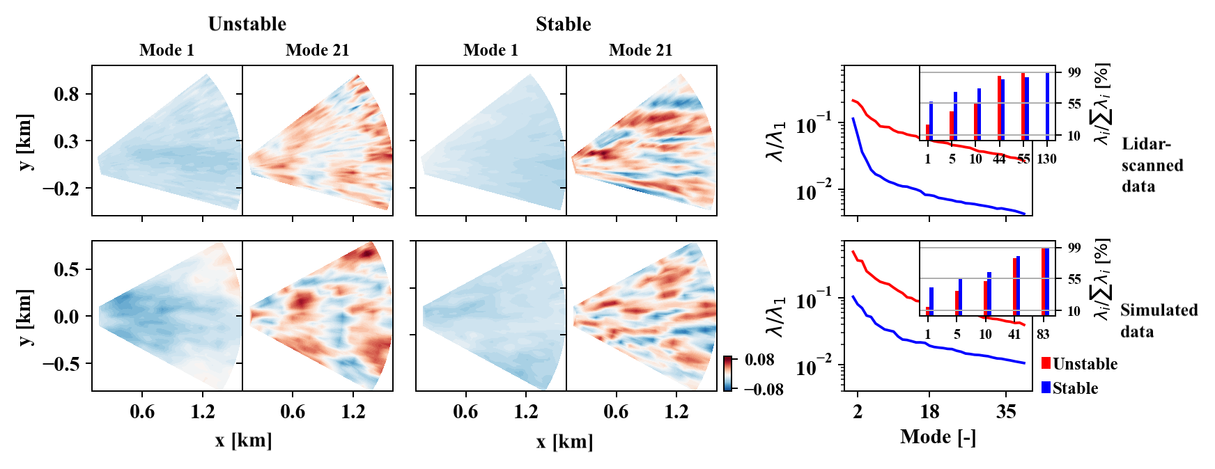
Figure 3Spatial POD modes 1 and 21 for the unstable (first and second columns) and stable (third and fourth columns) condition cases and POD energy (λ) among the first several modes (fifth column) and their cumulative energy (in the inset). Panels in the top and bottom rows represent the results from observed and the simulated data, respectively.
For both stability conditions, 90 east sectors, each 1 min apart, were selected from the simulations and used to compute the spatial proper orthogonal decomposition (POD) modes and energy (Berkooz et al., 1993). The actual lidar data for the unstable case uses 49 east sectors with wind speed and heat flux values similar to those in the simulations, 5–7 m s−1 and ∼ 350 W m−2, respectively. For the stable case, the actual lidar data employ 160 east sectors with a wind speed of 10–12 m s−1 and heat flux of W m−2, similar to the simulated values. Figure 3 shows the spatial POD modes 1 and 21 and the POD energy (λ, which denotes kinetic energy per unit mass of the flow) distributed among many modes for the simulated and actual lidar data for two stability conditions. The first POD mode in all cases shows the most significant coherent structures, followed by smaller structures for increasing mode numbers. For the given stability conditions, the simulated and lidar cases showed similar shape and size variations for all modes. The first few modes (modes < 5) show similar spatial structures in the POD modes for all stability conditions. However, they exhibit different spatial structures for the higher POD modes. For instance, mode 21 in the unstable case shows large open-cell-like structures, whereas mode 21 in the stable case shows streak-like structures oriented in the predominant wind direction. This variation in flow structures in different modes can be attributed to the forcing function. POD energy shown in Fig. 3 (right panels) depicts the turbulent energy associated with each coherent structure starting from mode 2. The unstable conditions consistently exceed the POD energy (for mode > 1) in both simulated and observed lidar data. The cumulative energy (Fig. 3, inset) indicates that the first mode of the stable condition case contains larger POD energy than the unstable condition case and requires larger modes to represent the energy in the flow in observational data. Although the trend of varying POD energy shows similarities between the two cases, the magnitude and the energy spread among the modes differ. Overall, the POD modes of the different stability cases demonstrate that the simulations capture the important features of coherent structures present in actual lidar data.
3.4 Complex-terrain case using 3D PBL
This second complex-terrain case also leverages measurements made during the WFIP2 campaign, which covered many stability conditions, including cold-air pools (CAPs) that tend to develop during synoptically quiescent periods. To study the ability of the 3D PBL scheme to capture such features, we chose a case from 10–20 January 2017 when a robust CAP was observed in the Columbia River Gorge. Such events are often challenging to represent accurately in mesoscale simulations due to the relatively small-scale boundary layer processes that must be parameterized. To better understand the spatial variability in meteorological and turbulence characteristics during the CAP lifecycle, we conducted WRF simulations following the High-Resolution Rapid Refresh (HRRR) reforecast configurations that were run for the WFIP2 project. For these simulations, the Mellor–Yamada–Nakanishi–Niino (MYNN; Nakanishi and Niino, 2006) scheme is run in the inner domain (horizontal grid cell spacing, Δ=750 m) of a nested two-domain setup. A novelty of this study is the use of NCAR's (National Center for Atmospheric Research) 3D PBL parameterization (Kosović et al., 2020; Juliano et al., 2022; Eghdami et al., 2022; Rybchuk et al., 2022), which was implemented into the WRF model for high-resolution mesoscale simulations. More information about the modeling setup and codes may be found in Mesoscale-to-Microscale Coupling (2023).
Several key findings emerged from the WFIP2 CAP study, with additional details reported by Arthur et al. (2022). First, turbulence kinetic energy (TKE) measurements from the profiling lidar at the Gordon's Ridge site reveal that, compared to MYNN, the 3D PBL simulation more accurately represents the vertical and temporal variability in TKE. As a result, wind speed errors were lower in the 3D PBL simulation, especially during the CAP erosion period, which has been especially difficult to model (Adler et al., 2021). To better understand the leading cause of the improved performance by the 3D PBL compared with MYNN, we performed a sensitivity analysis using the 3D PBL scheme framework. More specifically, we modified the turbulence closure approach as well as the turbulent length scale–closure constant formulation. The main reason for the improvement in TKE prediction is primarily related to the different turbulent length scale–closure constant formulation. For 3D PBL simulations under convective conditions, Juliano et al. (2022) reported similar findings regarding the primary importance of the turbulent length scale–closure constant formulation.
3.5 Offshore-wind case with a long offshore fetch
The MMC techniques developed for onshore studies were tested for a first offshore scenario at the FINO1 research tower, located in the North Sea. This case is representative of low roughness and low turbulence and leverage measurements from the FINO towers and data from the Alpha Ventus wind energy plant.
3.5.1 Comparison of coupling methods and turbulence generation methods
Comparisons are made between members of an ensemble of mesoscale simulations, different coupling methods with several models, and different turbulence generation schemes. The goal of the comparison is to assess the performance of each approach and highlight their strengths and weaknesses. The approaches compared include the following:
-
WRF to SOWFA (Simulator fOr Wind Farm Applications) using the indirect profile assimilation (IPA) technique,
-
WRF to SOWFA using the CPM at the inflow boundaries,
-
WRF to WRF-LES without any added turbulence generation (control simulation),
-
WRF to WRF-LES using the CPM at the inflow boundaries, and
-
WRF to WRF-LES using the Mann model to generate the large-scale turbulence.
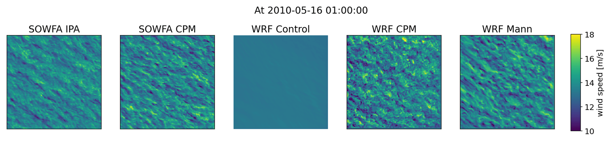
Figure 4Wind speed at 01:00 local time on 16 May 2010 around the FINO1 location for the different methods investigated. The original domains contain the fetch region. Shown here is a developed-turbulence 3×3 km subdomain.
The domains used were 6×6 km, with the exception of SOWFA IPA, which had a 3×3 km extent. All cases have a uniform 10 m grid resolution. Initial numerical experiments explored time-averaged vertical profiles at several locations in the fetch to determine an appropriate size. Convergence of vertical profiles of turbulent metrics was observed within a 3 km fetch distance. Thus, all the boundary-coupled scenarios considered were set up with a large 3 km extent fetch region to allow for turbulence development. The results shown here represent the developed-flow region, near the outlet boundaries. A qualitative visualization of the resulting flow field is given in Fig. 4.
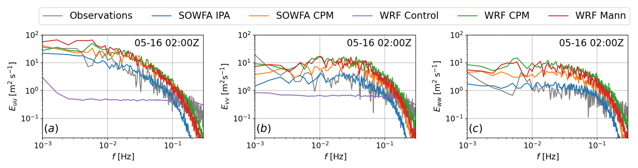
Figure 5Wind speed at 01:00 local time on 16 May 2010 around the FINO1 location for the different methods investigated. The original domains contain the fetch region. Shown here is a developed-turbulence 3×3 km subdomain.
Comparisons across the methods and observation data were made in terms of vertical profiles, power spectral density content, correlations, and integral scales. Figure 5 shows the energy spectrum during 1 h of the 4 h period of interest. The spectrum was obtained using 10 min Hamming windows with a 50 % overlap. To obtain smoother curves, we considered an ensemble average of several locations within the 3×3 km subdomain shown in Fig. 4, leveraging horizontal homogeneity. WRF Mann and both CPM methods overestimated the energy content, with the SOWFA IPA matching the content well with respect to observations up to a frequency related to the LES cutoff. The WRF control case showed very little content, as expected. The SOWFA IPA case is the only one where the turbulence was not triggered by a numerical method but rather developed using doubly periodic boundary conditions. All of the vertical profiles are comparable, with the exception of the control simulation, which due to the lack of resolved turbulence exhibited a larger shear profile. For a horizontal plane at 80 m, correlation maps were calculated for every point with respect to the central point, and correlation curves were obtained in the along-wind and cross-wind directions. Taylor's hypothesis was observed to be valid for this case, by means of spatial correlation and temporal autocorrelation. The correlation drop matched the correlation from observations well. The correlations dropped to zero faster in the cell perturbation method cases for both SOWFA and WRF-LES, which results in lower integral scales. Integration of the correlation curves yields the integral scales of the flow, shown in Fig. 6.
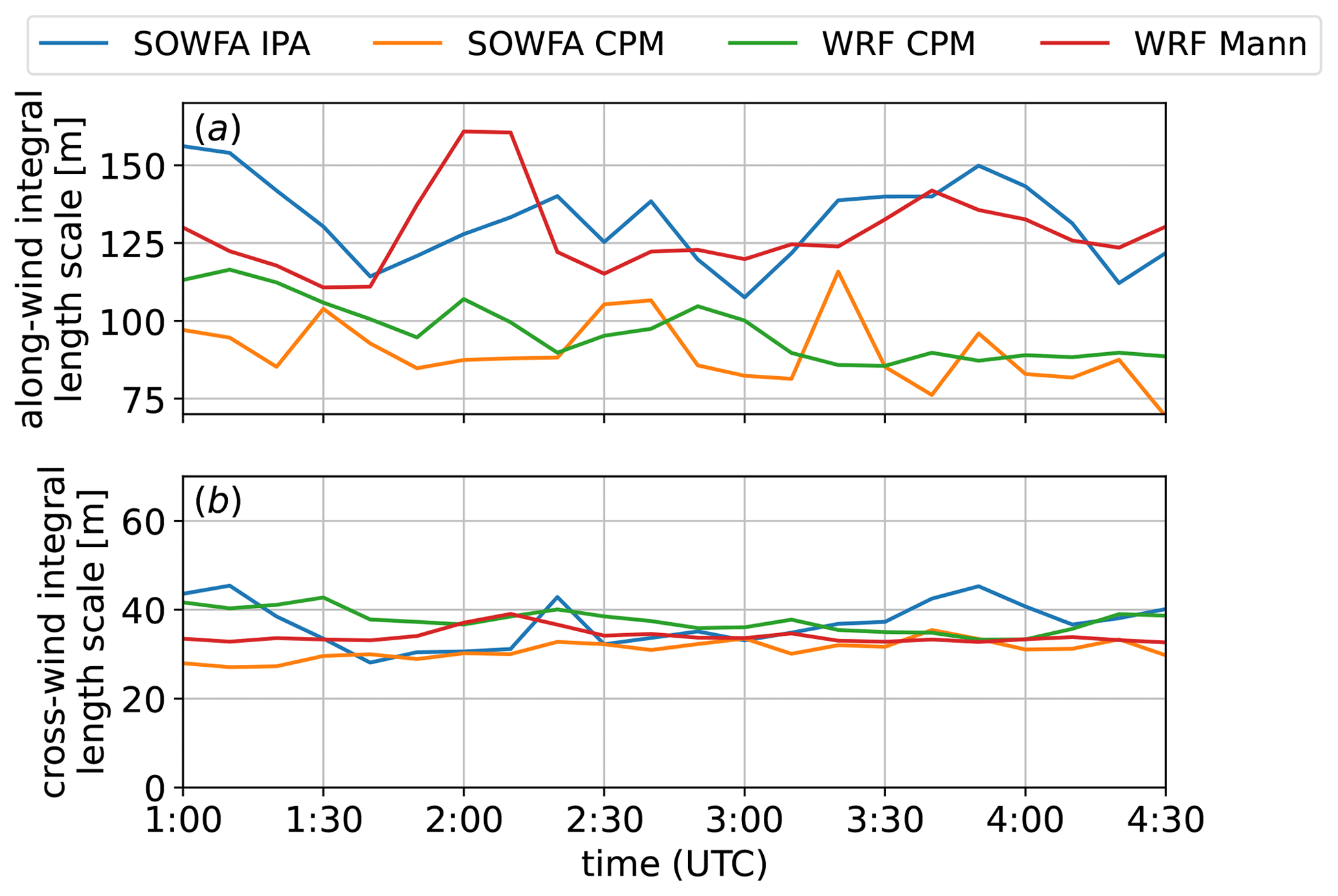
Figure 6Integral length scales calculated at 80 m in the along-wind and cross-wind directions for each coupling method.
The integral scales present in the cases that used the cell perturbation method to generate turbulence are smaller throughout the interval of interest. That is likely a result of the way the perturbation method works, by imposing small-scale disturbances in the temperature field, thus triggering high-frequency, small-scale turbulence that does little to change the integral scales of the flow as a whole. The Mann method, on the other hand, imposes large-scale turbulence, and the LES resolves the smaller scales. The larger scales imposed on the field are clearly observed when comparing the integral scales of the flow to those obtained using perturbation methods. Lastly, the SOWFA IPA case resulted in integral-scale values comparable to the Mann method in WRF-LES. For this SOWFA approach, the turbulence is developed by the use of periodic boundary conditions, which allows (in both space and time) for the development of large-scale structures, ultimately resulting in long correlation fetches and, thus, large values of the integral length scale. While the SOWFA IPA domain was overall smaller, it was nonetheless able to resolve scales of the order of 150 m as shown in Fig. 6. The integral scales in the cross-wind direction were of comparable magnitude in all cases investigated.
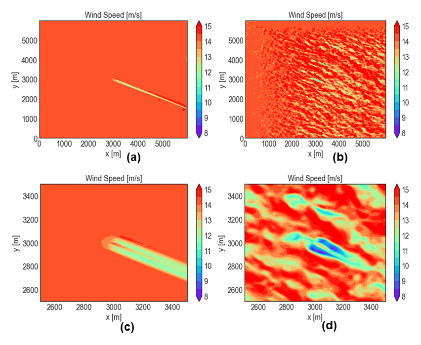
Figure 7Wind speed at 01:10:00 local time on 16 May 2010 in the domain containing the turbine (AV10) location using the WRF-LES-GAD approach for (a, c) no CPM and (b, d) CPM. The entire domain is shown in (a) and (b). A subset of the domain appears in (c) and (d).
3.5.2 The Alpha Ventus wind farm with a generalized actuator disk – turbine comparison
This section examines turbine wakes at the Alpha Ventus wind farm where the FINO1 tower is located and extends the analysis described in Sect. 3.5.1. WRF–WRF-LES and WRF–SOWFA coupling approaches were extended to include a wind turbine parameterization using a GAD formulation (Mirocha et al., 2014a). We refer to them as WRF-LES-GAD and WRF–SOWFA-GAD, and each compares using the CPM at the inflow boundaries vs. not adding any turbulence. The time window of interest is a 2 h window starting at 01:00 local time (00:00 UTC) on 16 May 2010. We consider a single turbine (AV10) for the purpose of this study.
Figure 7 presents a qualitative visualization of turbine wakes in the horizontal plane at hub height for the WRF-LES-GAD approach. As in Sect. 3.5.1, the LES domain is 6×6 km with a horizontal grid resolution of 10 m, which provides a large fetch as well as downstream distance for wake propagation. As expected, the simulation without the CPM does not resolve turbulence, and the resulting wake is what would be caused by an obstacle in the flow without any mixing. The simulation with the CPM includes resolved turbulence and hence mixing in the shear region, leading to a realistic wake. A comparison simulation using the WRF–SOWFA-GAD approach with the CPM (not shown) also concludes that modeling realistic wakes requires using a turbulence generation method.
3.6 Offshore US Northeast coastal case
A second offshore case is archived that studies the impact of different ways of representing surface roughness and providing sea surface boundary conditions. The offshore environment in the United States Northeast is an active area of research for wind energy development. Observations have recorded occurrences of persistent low-level jets (LLJs) with jet noses commonly below hub height (Debnath et al., 2021). In this study we assess the sensitivity of LLJ characteristics (e.g., jet nose height, maximum wind speed, low-level shear) to SST. We utilize six freely available satellite-derived SST datasets from the Group for High Resolution Sea Surface Temperature website (Table 1 and Fig. 8) to vary the lower boundary condition of surface temperature in online WRF simulations.
Table 1Sources of SST datasets used in this study. UKMO: UK Meteorological Office.
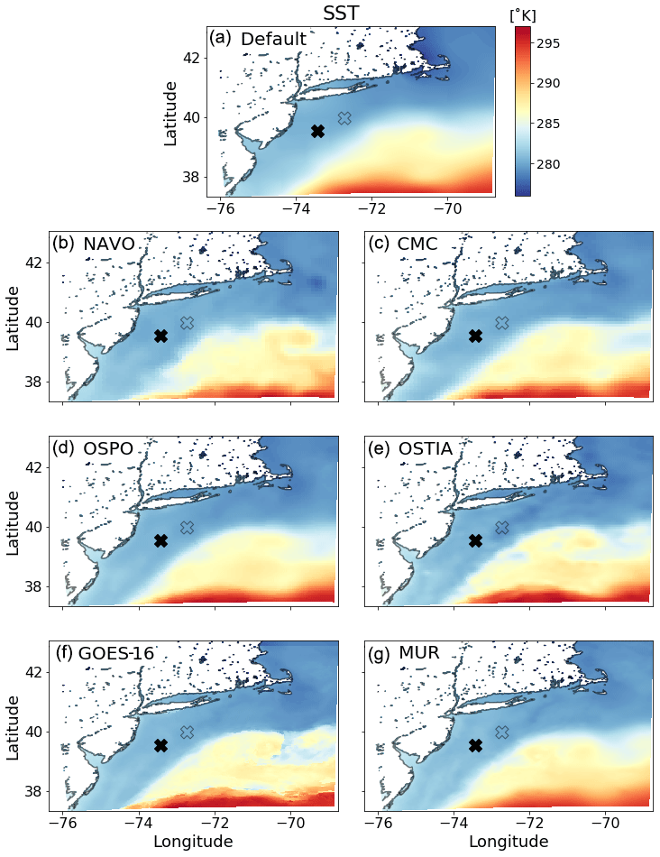
Figure 8Sea surface temperature datasets of varying resolution used as initial and surface boundary conditions over water.
The simulations consist of five domains with grid spacing spanning from 6250 down to 10 m. We used 88 vertical levels with 20 m spacing below 1 km. We compare model results against observations from the New York State Energy Research and Development Authority floating lidars. We assess model performance in capturing the LLJ nose height, maximum wind speed, and low-level shear on each domain in order to compare how sensitive the results are to SST on the mesoscale and microscale. With this comparison, we aim to determine whether model sensitivity on the mesoscale translates directly to the microscale. In other words, can we expect the best-performing mesoscale model setup to be the best setup on the microscale?
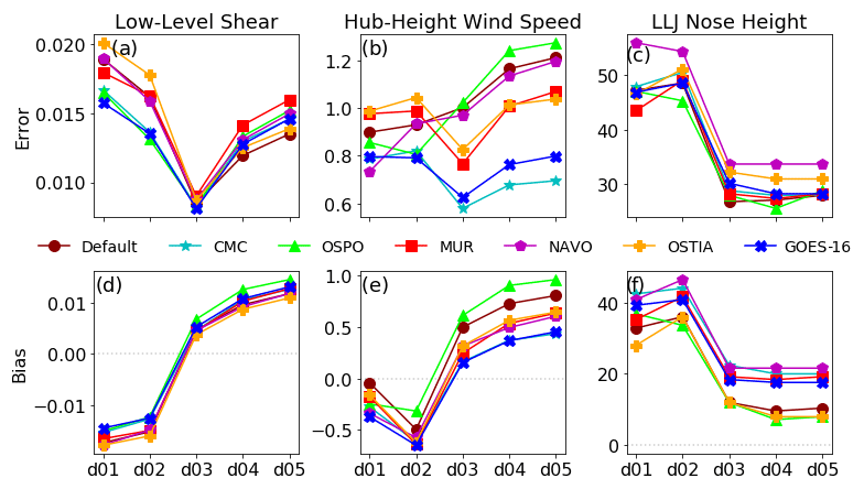
Figure 9(a, b, c) Error and (d, e, f) bias for each case on each domain for (a, d) low-level shear, (b, e) hub-height wind speed, and (c, f) LLJ height. Units for error are (a, d) per second, (b, e) meters per second, and (c, f) meters.
Results indicate that ensemble mean error and spread for various characteristics of the offshore LLJ vary between the mesoscale solutions and microscale solutions. However, variance within the microscale domains (domains 4 and 5) is small. The ensemble mean error of EME (where so is the observed quantity and is the ensemble mean) and bias of the low-level shear, hub-height wind speed (assumed to be at 118 m in this case), and jet nose height vary across scales from the mesoscale to the microscale (Fig. 9). Additionally, the best mesoscale performer did not lead to the best-performing microscale setup in this case when considering these metrics. On the mesoscale, the shear produced in the lowest levels was lower than what was observed. The LES results improved upon the low-level shear but overcorrected the lowest-level wind speeds and produced values lower than what were observed. It is suspected that using a drag force locally consistent with MOST within the heterogeneous microscale simulation is the root cause of this overcorrection of low-level winds. Future work must focus on generalizing this finding in order to determine if mesoscale simulations can inform performance on the microscale prior to running simulations.
The MMC team additionally tested ways to improve the models both in terms of improved physics as well as to test the efficacy of machine learning methods.
4.1 Three-dimensional planetary boundary layer parameterization
Traditional PBL schemes in mesoscale models are one-dimensional – that is, they parameterize only the vertical turbulent mixing under the assumption of horizontal homogeneity. In this sense, the vertical turbulent fluxes of momentum ( and ), potential temperature (), water vapor mixing ratio (), and any other relevant scalars (, where φ is a scalar variable, such as the cloud water mixing ratio) are computed. By definition, the horizontal homogeneity assumption neglects horizontal gradients in resolved quantities, as well as the vertical gradient in vertical velocity. Therefore, the vertical turbulent fluxes are dependent on only vertical gradients. However, this assumption is not justified at model resolutions in the terra incognita (Δ≈100–1000 m), where turbulence is partially resolved, and, thus, horizontal gradients play an important role (e.g., Kosović et al., 2021). A main consequence of ignoring horizontal gradients in the terra incognita and under convective conditions is the development of spurious structures (termed modeled convectively induced secondary circulations, or M-CISCs, by Ching et al., 2004), which can have a deleterious effect on the model solution. Furthermore, most 1D PBL parameterizations rely on the 2D horizontal diffusion scheme of Smagorinsky; however, this scheme was originally introduced for numerical stability and is therefore not physically motivated (Smagorinsky, 1990).
To address the fundamental research challenge of modeling in the terra incognita, our team has implemented the 3D PBL parameterization of Mellor and Yamada (Mellor, 1973; Mellor and Yamada, 1974, 1982) into the WRF model. This new parameterization does not impose the assumption of horizontal homogeneity; thus, it considers both vertical and horizontal gradients when computing all six momentum stresses and the full tensor for scalars (namely, θ and qv), in addition to all components of the flux divergences. As a result, this approach does not require the use of Smagorinsky's 2D horizontal diffusion scheme and shows promise at grid resolutions in the terra incognita, especially under convective conditions. To examine the influence of accounting for horizontal gradients, we set up different idealized model configurations under convective conditions and at a high-resolution mesoscale grid spacing (Δ=250 m). This grid spacing is considered to be mesoscale resolution because it is not fine enough to fully resolve the most energetic eddies (i.e., the LES limit) due to the model's effective resolution. The three single-domain, doubly periodic configurations are homogeneous surface forcing (rolls and cells), sea breeze front initiation, and mountain–valley circulation. Results clearly depict the suppression of M-CISCs by the 3D PBL scheme compared to a traditional 1D PBL scheme (Kosović et al., 2021; Juliano et al., 2022). The impact of the turbulent length scale–closure constant formulation is found to be very important, such that M-CISCs may be present in the 3D PBL solution when the length scale is insufficiently large and thus vertical mixing is not strong enough. In general, we believe that the 3D PBL parameterization has the potential to be useful both as a mesoscale-only approach and as part of a mesoscale–microscale coupling strategy.
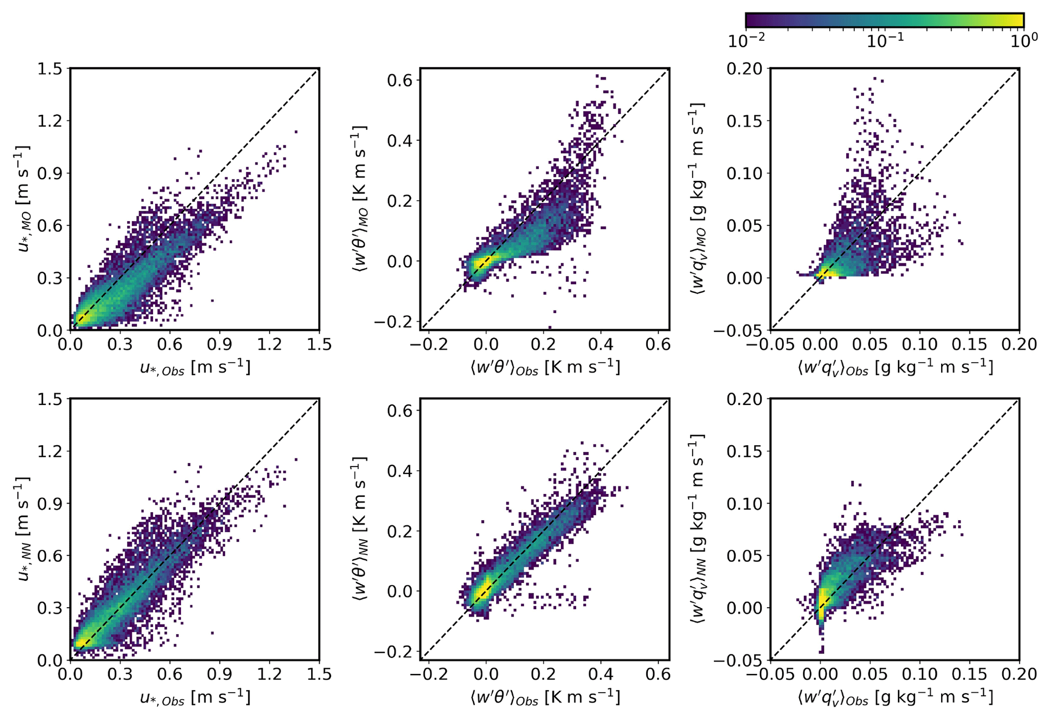
Figure 10Comparison of the MOST (top row) and an offline NN model (bottom row) surface-layer parameterizations of surface friction velocity (left panels), sensible heat flux (middle panels), and moisture flux (right panels) with observations from the Cabauw mast. Figure originally appeared in Muñoz-Esparza et al. (2022).
4.2 Machine learning surface-layer scheme
Specifying lower boundary conditions in numerical simulations of high-Reynolds-number atmospheric boundary layer flows requires estimating turbulent fluxes of momentum, heat, moisture, and other constituents. However, these fluxes are not known a priori and therefore must be parameterized. Parameterization of surface fluxes in atmospheric-flow models at any scale, from global to turbulence-resolving large-eddy simulations, are based on MOST where atmospheric-stability effects are accounted for through universal, semi-empirical stability functions. The stability functions are a function of the nondimensional stability parameter, a ratio of distance from the surface and the Obukhov length scale (Monin and Obukhov, 1954). However, their functional form is determined based on observations using simple regression that cannot represent the surface-layer structure and governing parameters under a wide range of conditions. We have therefore developed and tested a neural network (NN) ML model for surface-layer parameterization (McCandless et al., 2022). We trained and tested the ML model using long-term observations from the National Oceanic and Atmospheric Administration's Field Research Division tower in Idaho and the Cabauw mast in the Netherlands. The offline comparison of MOST and the NN model surface-layer parameterizations with observations from the Cabauw mast are shown in Fig. 10. We then implemented the ML model in the FastEddy GPU-native LES model (Muñoz-Esparza et al., 2022) and the WRF single-column model. The ML model implementation in FastEddy demonstrates that it can accurately capture the diurnal evolution of an atmospheric boundary layer as shown in Fig. 11.
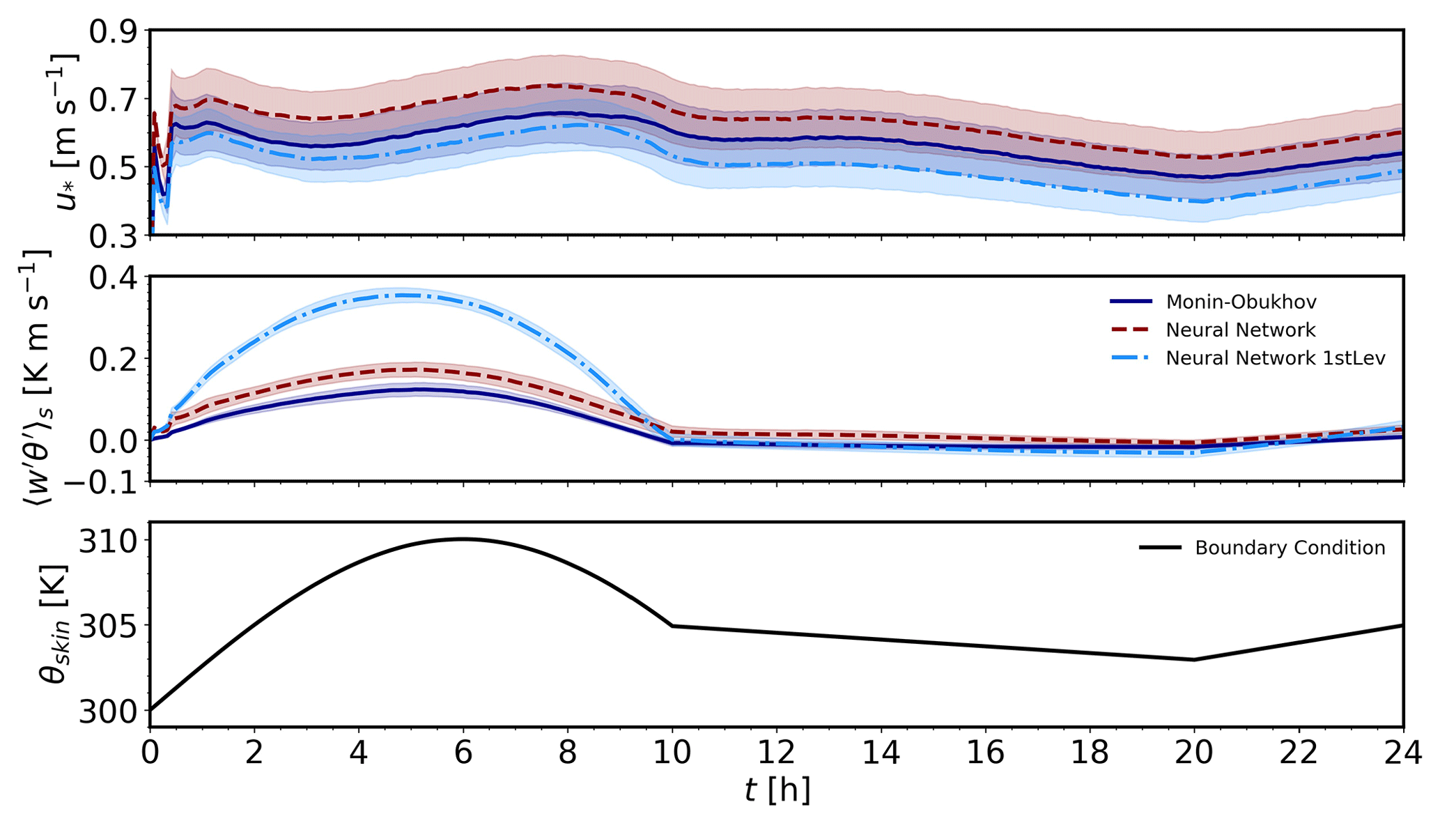
Figure 11Comparison of the diurnal evolution of an ABL using the FastEddy LES model with the MOST and NN model surface-layer parameterizations: surface friction velocity (top panel), sensible heat flux (second panel), moisture flux (third panel), and boundary forcing from surface skin temperature (bottom panel). The shaded areas show 1 standard deviation from the mean over the simulation domain. Figure originally appeared in Muñoz-Esparza et al. (2022).
The ML model implementation in the WRF model was tested using a single-column model (SCM) based on the GABLS3 intercomparison study case defined by Bosveld et al. (2014). The comparison of SCM simulations using the ML model surface-layer parameterization with observations and the MOST parameterization demonstrates that it can capture the sensible heat flux, the skin temperature, the surface friction velocity, and the planetary boundary layer height well but underestimates the latent heat flux (Fig. 12).
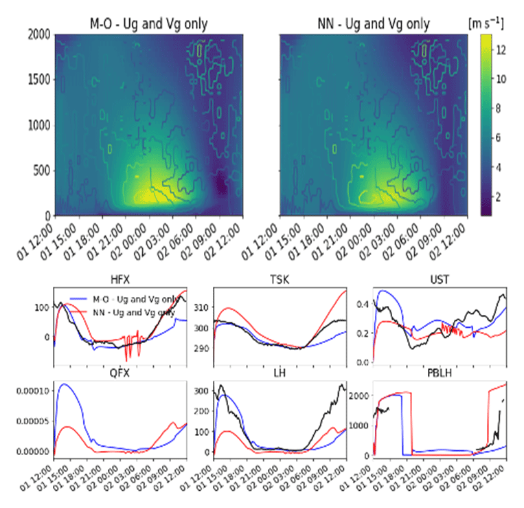
Figure 12Output from the SCM simulation of a GABLS3 intercomparison study case using an idealized WRF model. The figure compares WRF simulations using MOST (M-O) and a neural network (NN) parameterization. The black line shows the observed data from GABLS3 (Cabauw) for comparison. “Ug and Vg only” refers to the single-column simulations only being forced by changes to the geostrophic wind. The bottom portion of the figure shows heat flux (HFX), skin temperature (TSK), u* (UST), moisture flux (QFX), latent heat (LH), and PBL height (PBLH).
A potential reason for discrepancies between the ML-model-predicted and observed latent heat flux is that the ML model for the surface-layer parameterization implemented in WRF interacts with a land–surface model, which is based on MOST.
The ML model for surface-layer parameterization demonstrates the potential to provide better estimates of surface fluxes in comparison to commonly used MOST-based parameterizations. However, to develop a generally applicable ML model it must be trained using long-term, consistent, complete, and quality-controlled observations from a wide range of environments. Future research could focus on expanding the training dataset and testing the model in mesoscale simulations over diverse locations.
4.3 Downscaling with deep learning
Microscale simulations, like WRF-LES (30 m), generated over the Columbia River basin for the Wind Forecast Improvement Project 2 (WFIP2), are able to model the very complicated flow associated with complex terrain including downslope flows, mountain wakes, mountain–valley circulations, gravity waves, cold pools, and gap flows. However, such simulations are currently too complex to configure and computationally expensive for use outside the scientific research community. Here we tested using deep artificial neural networks on the LES to directly downscale from the mesoscale to the microscale in complex terrain. Once trained, deep learning models can generate high-resolution simulations from a coarse image in just a few seconds from mesoscale input. In addition, we wished to demonstrate that the deep network models can then potentially be applied to regions other than the LES domain on which they were trained.
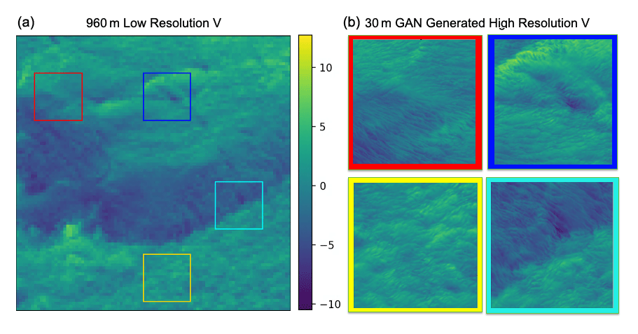
Figure 13Example of using the GAN to downscale from (a) a coarsened 960 m resolution simulation to (b) four example panels showing high-resolution 30 m generated images. The colors overlaid on (a) correspond to the same color outlined image on (b).
We created high-resolution–low-resolution training sample pairs by subtiling relevant vertical levels of the LES on the eastern portion of the domain and coarsening the tiles with average filters. We trained two separate enhanced super-resolution generative adversarial networks (ESRGANs; Ledig et al., 2017; Wang et al., 2018) to accomplish the downscaling by training one GAN to downscale from 960 to 240 m and the second GAN to downscale from 240 to 30 m and applying the models successively. We set aside data from every third time step in the LES for testing. Visually, the performance of the compound GAN architecture on testing data samples and the larger domain was impressive (Fig. 13). We performed statistical analysis of the high-resolution GAN-generated wind and compared it with the LES, finding good agreement in the power spectra, velocity gradient distributions, and wind speed and wind direction distributions (Dettling et al., 2023). We found high Pearson correlation coefficients and very low mean bias between the tiles of GAN-generated wind components and LESs, as well as good agreement in the moments of GAN-generated wind components with the LES, even in the higher-order moments, skewness, and kurtosis (Dettling et al., 2023).
To demonstrate the potential of transfer learning, we extended the testing sample set to include the western half of WRF-LES, which contains part of the Cascade Range including Mt. Hood. The western region is not only very unique when compared to the training region in the east but also topographically much more complex. We performed the same statistical analysis to compare the GAN-generated wind to the LES in the transfer learning region, and the results were encouraging (Dettling et al., 2023).
We have summarized the results of the U.S. Department of Energy-sponsored (DOE) Mesoscale to Microscale Coupling (MMC) project that has focused on the best ways to couple the mesoscale to the microscale in order to better understand and model the transfer of energy from the largest scales of the atmosphere to those scales that directly affect harvesting that energy via wind turbines. The approach of using case studies based on observations has been a productive approach to test methodologies and has kept the findings grounded in real-world atmospheric behavior. The approach has required that we choose progressively more difficult cases, bringing in real-world complexity to better understand the implications of that complexity and how to best model it. We have studied how the mesoscale setup impacts the microscale results, applying consistent and appropriate boundary conditions, multiple methods of applying the coupling between scales, bridging the terra incognita, initializing turbulence at the microscale that is not resolved at the mesoscale, and applying these methods in complex terrain and in coastal and offshore environments. We additionally explored improving model parameterization (3D PBL and an ML-based surface-layer model) and demonstrated deep learning methods for downscaling from the mesoscale to the microscale. It is important to apply assessment metrics that are most appropriate for uses in wind energy, considering more than merely mean winds but also sheer, veer, turbulence intensity, and turbulent kinetic energy via metrics such as energy spectra, PDFs (probability density functions) along the flow, covariance, and proper orthogonal decomposition.
Some specific lessons learned include the following:
-
Microscale simulations cannot necessarily improve matches to measurements if forced with an inaccurate mesoscale simulation (Sect. 3.1).
-
Idealized simulations may not represent real-world phenomena well and may be more difficult to initialize well than real cases.
-
Microscale data assimilation (through profile assimilation on a periodic domain) requires an approach that allows for the microscale to deviate from the mesoscale; otherwise wind and temperature profiles may not be in the correct equilibrium, resulting in unrealistic turbulence (Allaerts et al., 2020, 2023).
-
High-quality potential temperature profiles, in addition to wind profiles, are necessary when performing microscale data assimilation with observational data (Allaerts et al., 2023; Jayaraman et al., 2022; Quon, 2023).
-
Accurately capturing transitional atmospheric boundary layers and intermittent stable boundary layers remains a challenge (Allaerts et al., 2023; Quon, 2023).
-
Without coupling across scales, even mesoscale flow is underresolved (Rai et al., 2019).
-
Proper orthogonal decomposition analysis clearly indicates that the microscale contains energetic modes that originated from the mesoscale flow (Rai et al., 2019).
-
The upper limit of the terra incognita is the boundary layer depth, indicating that horizontal spacing smaller than that (but larger than about 100 m) is likely to result in spurious secondary structures (Rai et al., 2019).
-
Spurious roll features from the terra incognita can translate into unrealistic flow in the microscale (Rai et al., 2019).
-
Turbulence generation methods are necessary to avoid long fetches in developing turbulence at the microscale that is not resolved at the mesoscale (Sect. 2.4).
-
Temperature perturbation methods create turbulent fields with artificially small integral scales (Sect. 3.5)
-
Uncertainty can typically be traced to a small number of model parameters, and the importance of these specific parameters can be interpreted in terms of flow physics considerations (Sect. 2.5).
-
Certain conditions, such as complex terrain, can force gravity waves that reflect off of boundaries and grow to spurious amplitudes. Such gravity waves can be mitigated by Rayleigh damping (Sect. 2.6.2).
-
The best mesoscale simulations do not always translate to the best match to wind-relevant metrics for the microscale simulation (Sect. 3.6).
-
A three-dimensional planetary boundary layer scheme can alleviate M-CISCs in the terra incognita (Sect. 4.1; Juliano et al., 2022).
Much research remains to be done to continue to enhance our understanding of the scales of atmospheric motion most relevant for harvesting wind energy. This team and the community have more work to do on the plethora of complex cases. More research is needed to further improve coupling technologies. For instance, more research is needed to understand why direct/indirect profile assimilation is successful in some cases and unsuccessful in others. We should also continue to explore topics of complexity, both onshore and offshore. Much remains to be learned through judiciously applying uncertainty quantification methods.
Although the current A2e MMC project has formally ended, we expect that its impact will live on, both in terms of providing code and methodologies that can be used by a wide range of wind farm modelers and in terms of being integrated into subsequent DOE wind energy projects. Specifically, the DOE is initiating projects in offshore wind energy, complex-terrain modeling for wind energy, and the impact of extreme events on modeling for wind energy.
In deploying renewable energy, we have become more cognizant of issues of fairness and justice to the people being impacted. In the United States, the Biden administration's Justice40 Initiative (White House, 2022), which seeks to deliver 40 % of the overall benefits of climate investments to disadvantaged communities and inform equitable research, development, and deployment within the DOE, has recently highlighted the importance of energy justice considerations within the development of new energy systems. One of the major challenges of working in this space is finding actionable, effective paths forward while acknowledging and respecting the existing legacy of noninclusivity. Organizations such as the Initiative for Energy Justice and the Energy Equity Project (Initiative for Energy Justice, 2022) have established guidelines for working in the space of energy justice. Specifically these include addressing the current perceptions that have been built on past practices, identifying uniquely disadvantaged people, promoting procedural fairness, making sure that access is equally tenable, making sure the quality of service is equal across groups, and ensuring the desired impacts. Defined metrics can be used to determine whether or not a project is successful in working toward energy justice. While fairly centered on policymaking, these assessment points can help guide the focus of renewable energy development and act as a compass for what research objectives will have a meaningful impact.
Finally, the MMC team wishes to thank colleagues and community members for input throughout the course of this project. Our industry advisory panel and attendees to our various webinars and workshops have provided valuable input as to the directions that we have chosen and solutions that may be most practical for application to real-world needs. The biggest lesson learned is that it is through community cooperation that we are most likely to advance the science and technology needed to deploy the amounts of wind energy that the world will need for a carbon-free energy future.
The team has archived simulation codes and model workflows for a range of case studies that can be used as a starting point for users to develop their own applications. The MMC version of the WRF code is at https://doi.org/10.5281/zenodo.7765891 (Gill et al., 2023) and WRF setups at https://doi.org/10.5281/zenodo.7766133 (Hawbecker et al. 2023b). SOWFA input decks are at https://doi.org/10.5281/zenodo.7764348 (Quon et al., 2023c). Python utilities for data analysis, simulation setup, and postprocessing are at https://doi.org/10.5281/zenodo.7768674 (Quon et al., 2023b). Jupiter notebooks for assessment are at https://doi.org/10.5281/zenodo.7768670 (Quon, et al., 2023a). Online documentation resides in a “Read the Docs” format (Mesoscale-to-Microscale Coupling, 2023, https://mmc.readthedocs.io/en/latest/).
Data for the flat and complex terrain cases are available on DOE's Wind Data Hub (https://a2e.energy.gov/data#ProjectFilter=["wfip2"], DOE, 2023). Datasets of differing SSTs used for the offshore US Northeast coast case study are available from NASA (2018) (https://doi.org/10.5067/GHK10-L4N01), CMC (2017) (https://doi.org/10.5067/GHCMC-4FM03), OSPO (2015) (https://doi.org/10.5067/GHGPB-4FO02), UKMO (2005) (https://doi.org/10.5067/GHOST-4FK01), NOAA (2019) (https://doi.org/10.5067/GHG16-3UO27), and NASA (2015) (https://doi.org/10.5067/GHGMR-4FJ04).
This paper results from a team effort to which all authors contributed. Project oversight and leadership plus management coordination was led by SEH with assistance from BK, LKB, CMK, JM, and MC. SD and MR provided oversight and resources from the DOE, with MR providing overarching research goals and aims. EQ and PH led the software and data curation, with assistance from other authors. SEH led the preparation of the manuscript and all authors contributed.
The contact author has declared that none of the authors has any competing interests.
Publisher’s note: Copernicus Publications remains neutral with regard to jurisdictional claims in published maps and institutional affiliations.
This work was authored in part by the National Renewable Energy Laboratory, operated by the Alliance for Sustainable Energy, LLC, for the U.S. Department of Energy (DOE) (contract no. DE-AC36-08GO28308); Pacific Northwest National Laboratory (PNNL), operated by the Battelle Memorial Institute, for the U.S. DOE (contract no. DE-A06-76RLO 1830); and Lawrence Livermore National Laboratory, operated by Lawrence Livermore National Security, for the U.S. DOE (contract no. DE-AC52-07NA27344). Funding was provided by the U.S. Department of Energy Office of Energy Efficiency and Renewable Energy Wind Energy Technologies Office. The views expressed in the article do not necessarily represent the views of the DOE or the U.S. Government. The U.S. Government retains and the publisher, by accepting the article for publication, acknowledges that the U.S. Government retains a nonexclusive, paid-up, irrevocable, worldwide license to publish or reproduce the published form of this work or allow others to do so for U.S. Government purposes. The National Center for Atmospheric Research (NCAR) was a subcontractor to the PNNL. NCAR is a major facility sponsored by the National Science Foundation (cooperative agreement no. 1852977). The authors wish to thank the reviewers whose comments and suggestions resulted in an improved paper.
This research has been supported by the Wind Energy Technologies Office (grant nos. DE-A06-76RLO 1830, DE-AC36-08GO28308, and DE-AC52-07NA27344).
This paper was edited by Julia Gottschall and reviewed by Javier Sanz Rodrigo and one anonymous referee.
Adler, B., Wilczak, J. W., Bianco, L., Djalalova, I., Duncan Jr., J. B., and Turner, D.: Observational case study of a persistent cold pool and gap flow in the Columbia River basin, J. Appl. Meteorol. Clim., 60, 1071–1090, https://doi.org/10.1175/JAMC-D-21-0013.1, 2021.
Allaerts, D., Quon, E., Draxl, C., and Churchfield, M.: Development of a Time-Height Profile Assimilation Technique for Large-Eddy Simulation, Bound.-Lay. Meteorol., 176, 329–348, https://doi.org/10.1007/s10546-020-00538-5, 2020.
Allaerts, D., Quon, E., and Churchfield, M.: Using observational mean-flow data to drive large-eddy simulations of a diurnal cycle at the SWiFT site, Wind Energ., 126, 469–492, https://doi.org/10.1002/we.2811, 2023.
Arthur, R. S., Mirocha, J. D., Lundquist, K. A., and Street, R. L.: Using a canopy model framework to improve large-eddy simulations of the atmospheric boundary layer in the Weather Research and Forecasting model, Mon. Weather Rev., 147, 31–52, https://doi.org/10.1175/MWR-D-18-0204.1, 2019.
Arthur, R. S., Mirocha, J. D., Marjanovic, N., Hirth, B. D, Schroeder, J. L., Wharton, S., and Chow, F. K.: Multi-scale simulation of wind farm performance during a frontal passage, Atmosphere, 11, 245, https://doi.org/10.3390/atmos11030245, 2020.
Arthur, R. S., Juliano, T. W., Adler, B., Krishnamurthy, R., Lundquist, J. K., Kosović, B., and Jiménez, P. A.: Improved representation of horizontal variability and turbulence in mesoscale simulations of an extended cold-air pool event, J. Appl. Meteorol. Clim., 61, 685–707, https://doi.org/10.1175/JAMC-D-21-0138.1, 2022.
Berg, L. K., Liu, Y., Yang, B., Qian, Y., Olson, J., Ma, P.-L., and Hou, Z.: Sensitivity of turbine-height wind speeds to parameters in the planetary boundary-layer parametrization used in the Weather Research and Forecasting model: Extension to wintertime conditions, Bound.-Lay. Meteorol., 170, 507–518, https://doi.org/10.1007/s10546-018-0406-y, 2019.
Berkooz, G., Holmes, P., and Lumley, J. L.: The proper orthogonal decomposition in the analysis of turbulent flows, Annu. Rev. Fluid Mech., 25, 539–575, https://doi.org/10.1146/annurev.fl.25.010193.002543, 1993.
Bosveld, F. C., Baas, P., van Meijgaard, E., de Bruijn, E. I. F., Steeneveld, G.-J., and Holtslag, A. A. M.: The Third GABLS Intercomparison Case for Evaluation Studies of Boundary-Layer Models. Part A: Case Selection and Set-Up, Bound.-Lay. Meteorol., 152, 133–156, https://doi.org/10.1007/s10546-014-9919-1, 2014.
Bou-Zeid, E., Meneveau, C., and Parlange, M. B.: A scale-dependent Lagrangian dynamic model for large eddy simulation of complex turbulent flows, Phys. Fluids, 17, 025105, https://doi.org/10.1063/1.1839152, 2005.
Brasseur, J. G. and Wie, T: Designing large-eddy simulation of the turbulent boundary layer to capture law-of-the-wall scaling, Phys. Fluids, 22, 021303, https://doi.org/10.1063/1.3319073, 2010.
Brown, A. R., Hobson, J. M., and Wood, N.: Large-eddy simulation of neutral turbulent flow over rough sinusoidal ridges, Bound.-Lay. Meteorol., 98, 411–441, https://doi.org/10.1023/A:1018703209408, 2001.
Canada Meteorological Center (CMC): GHRSST Level 4 CMC0.1deg Global Foundation Sea Surface Temperature Analysis (GDS version 2), Canada Meteorological Center [data set], https://doi.org/10.5067/GHCMC-4FM03, 2017.
Ching, J., Rotunno, R., LeMone, M., Martilli, A., Kosović, B., Jiménez, P. A., and Dudhia, J.: Convectively induced secondary circulations in fine-grid mesoscale numerical weather prediction models, Mon. Weather Rev., 142, 3284–3302, https://doi.org/10.1175/MWR-D-13-00318.1, 2014.
Chow, F. K., Street, R. L., Xue, M., and Ferziger, J. H.: Explicit filtering and reconstruction turbulence modeling for large-eddy simulation of neutral boundary layer flow, J. Atmos. Sci., 62, 2058–2077, https://doi.org/10.1175/JAS3456.1, 2004.
Churchfield, M. J., Lee, S., Moriarty, P. J., Martínez, L. A., Leonardi, S., Vijayakumar, G., and Brasseur, J. G.: A large-eddy simulation of wind-plant aerodynamics, 50th AIAA Aerospace Sciences Meeting Including the New Horizons Forum and Aerospace Exposition, 9–12 January 2012, Nashville, Tennessee, https://doi.org/10.2514/6.2012-537, 2012.
Debnath, M., Doubrawa, P., Optis, M., Hawbecker, P., and Bodini, N.: Extreme wind shear events in US offshore wind energy areas and the role of induced stratification, Wind Energ. Sci., 6, 1043–1059, https://doi.org/10.5194/wes-6-1043-2021, 2021.
Dettling, S., Brummet, T., Gagne, D. J., Kosovic, B., and Haupt, S. E.: Downscaling from Mesoscale to Microscale in Complex Terrain using a Generative Adversarial Network, in preparation, 2023.
DOE: The Wind Data Hub, A2EDAP (Atmosphere to Electrons (A2e), Data Archive and Portal [data set], https://a2e.energy.gov/data#ProjectFilter=["wfip2"] (last access: 11 August 2023), 2023.
Draxl, C., Allaerts, D., Quon, E., and Churchfield, M.: Coupling Mesoscale Budget Components to Large-Eddy Simulations for Wind-Energy Applications, Bound.-Lay. Meteorol., 179, 73–98, https://doi.org/10.1007/s10546-020-00584-z, 2021.
Eghdami, M., Barros, A. P., Jiménez, P. A., Juliano, T. W., and Kosovic, B.: Diagnosis of Second-Order Turbulent Properties of the Surface Layer for Three-Dimensional Flow Based on the Mellor–Yamada Model, Mon. Weather Rev., 150, 1003–1021, https://doi.org/10.1175/MWR-D-21-0101.1, 2022.
Gill, D., Dudhia, J., Wang, W., Peckham, S., Bresch, J., Kavulich, M., Black, T., Carson, L., Zhang, X., Werner, K., Hawbecker, P., Huang, W., Manning, K., Duda, M., Walters, S., Zhiquan, J., Jha, P., Juliano, T. Guerrette, J. J., Jimenez, P., and Munoz-Esparza, D.: MMC-WRF, a2e-mmc/WRF: End of A2e MMC Project (v4.3), Zenodo [code], https://doi.org/10.5281/zenodo.7765891, 2023.
Gopalan, H., Gundling, C., Brown, K., Roget, B. Sitaraman, J., Mirocha, J. D., and Miller, W. O.: A Coupled Mesoscale-Microscale Framework for Wind Resource Estimation and Farm Aerodynamics, J. Wind Eng. Ind. Aerodyn., 132, 13–26, https://doi.org/10.1016/j.jweia.2014.06.001, 2014.
Haupt, S. E., Kosovic, B., Shaw, W., Berg, L., Churchfield, M., Cline, J., Draxl, C., Ennis, B., Koo, E., Kotamarthi, R., Mazzaro, L., Mirocha, J., Moriarty, P., Munoz-Esparza, D., Quon, E., Rai, R. K., Robinson, M., and Sever, G.: On Bridging a Modeling Scale Gap: Mesoscale to Microscale Coupling for Wind Energy, B. Am. Meteorol. Soc., 100, 2533–2549, https://doi.org/10.1175/BAMS-D-18-0033.1, 2019a.
Haupt, S. E., Allaerts, D., Berg, L., Churchfield, M., DeCastro, A., Draxl, C., Gagne, D. J., Hawbecker, P., Jimenez, P., Jonko, A.,. Juliano, T., Kaul, C., Kosovic, B., McCandless, T., Mirocha, J., Munoz-Esparza, D., Quon, E., Rai, R., Sauer, J., and Shaw, W.: FY19 Report of the Atmosphere to Electrons Mesoscale to Microscale Coupling Project: Pacific Northwest Laboratory Report PNNL-29603, 127 pp., https://doi.org/10.2172/1735568, 2019b.
Haupt, S. E., Arthur, R., Berg, L., Churchfield, M., DeCastro, A., Dettling, S., Draxl, C., Gagne, D. J., Hawbecker, P., Jimenez, P., Jonko, A., Juliano, T., Kaul, C., Kosovic, B., Lassman, Kumar, M., McCandless, T. C., Mirocha, J., Quon, E., Rai, R., Shaw, W., and Thedin, R.: FY20 Report of the Atmosphere to Electrons Land-Based Mesoscale to Microscale Coupling Project: Pacific Northwest Laboratory Report PNNL-30841, 104 pp., https://www.osti.gov/servlets/purl/1762812 (last access: 6 August 2023), 2020.
Hawbecker, P. and Churchfield, M.: Evaluating Terrain as a Turbulence Generation Method, Energies, 14, 6858, https://doi.org/10.3390/en14216858, 2021.
Hawbecker, P., Lassman, W., Juliano, T. W., Kosivic, B., and Haupt, S. E.: Model sensitivity across scales, in preparation, 2023a.
Hawbecker, P., Quon, E., Jha, P., Sauer, J., Rai, R., Juliano, T., and Lassman, W.: WRF Setups, a2e-mmc/WRF-setups: End of A2e MMC Project (v1.0), Zenodo [data set] and [code], https://doi.org/10.5281/zenodo.7766133, 2023b.
Initiative for Energy Justice: https://iejusa.org/, last access: 30 November 2022.
Jayaraman, B., Quon, E., Li, J., and Chatterjee, T.: Structure of offshore low-level jet turbulence and implications to mesoscale-to-microscale coupling, Journal of Phyasics: Conference Series, The Scientce of Making Torque from Wind (TORQUE 2022), 2265, 022064, https://doi.org/10.1088/1742-6596/2265/2/022, 2022.
Jiménez, P. A. and Dudhia, J.: On the need to modify the sea surface roughness formulation over shallow waters, J. Appl. Meteorol. Climatol., 57, 1101–1110, 2018.
Jonkman, B. J.: TurbSim user's guide, No. NREL/TP-500-39797, National Renewable Energy Lab (NREL), Golden, CO (United States), 2006.
Juliano, T. W., Kosović, B., Jiménez, P. A., Eghdami, M., Haupt, S. E., and Martilli, A.: Gray zone simulations using a three-dimensional planetary boundary layer parameterization in the Weather Research and Forecasting model, Mon. Weather Rev., 150, 1585–1619, https://doi.org/10.1175/MWR-D-21-0164.1, 2022.
Kaul, C. M., Ananthan, S., Churchfield, M. J., Mirocha, J. D., Berg, L. K., and Rai, R.: Large-eddy simulations of idealized atmospheric boundary layers using Nalu-Wind, J. Phys. Conf. Ser., 1452, 012078, https://doi.org/10.1088/1742-6596/1452/1/012078, 2020.
Kaul, C. M., Hou, Z. J., Zhou, H., Rai, R. K., and Berg, L. K.:. Sensitivity analysis of wind and turbulence predictions with mesoscale-coupled large eddy simulations using ensemble machine learning, J. Geophys. Res.-Atmos., 127, e2022JD037150, https://doi.org/10.1029/2022JD037150, 2022.
Kelley, C. L. and Ennis, B. L.: SWiFT site atmospheric characterization (No. SAND2016-0216), Sandia National Laboratories, Albuquerque, NM, https://doi.org/10.2172/1237403, 2016.
Kelley, N. D.: Turbulence-Turbine Interaction: The Basis for the Development of the TurbSim Stochastic Simulator, NREL/TP-5000-52353, https://doi.org/10.2172/1031981, 2011.
Khani, S. and Porté-Agel, F.: A modulated-gradient parametrization for the large eddy simulation of the atmospheric boundary layer using the Weather Research and Forecasting model, Bound.-Lay. Meteorol., 165, 385–404, 2017.
Kirkil, G., Mirocha, J. D., Bou-Zeid, E., Chow, F. K., and Kosović, B.: Implementation and Evaluation of Dynamic Subfilter-Scale Stress Models for Large-Eddy Simulation using WRF, Mon. Weather Rev., 140, 266–284, https://doi.org/10.1175/MWR-D-11-00037.1, 2012.
Kosović, B., Munoz, P. J., Juliano, T. W., Martilli, A., Eghdami, M., Barros, A. P., and Haupt, S. E.: Three-dimensional planetary boundary layer parameterization for high-resolution mesoscale simulations, Journal of Physics: Conference Series, IOP Publishing, 1452, 012080, https://doi.org/10.1088/1742-6596/1452/1/012080, 2020.
Kosović, B., Jimenez, P. A., Juliano, T. W., Eghdami, M., and Haupt, S. E.: Analysis of Horizontal Shear and Mixing at Gray Zone Length Scales Using Filtered Large-Eddy Simulation of a Flow over Complex Terrain, in: 101st American Meteorological Society Annual Meeting, AMS, https://ui.adsabs.harvard.edu/abs/2020AGUFMGC0590002K/abstract (last access: 6 August 2023), 2021.
Ledig, C., Theis, L., Huszar, F., Caballero, J., Cunningham, A., Acosta, A., Aitken, A., Tejani, A., Totz, J., Wang, Z., and Shi, W.: Photo-Realistic Single Image Super-Resolution Using a Generative Adversarial Network, arXiv [preprint], https://doi.org/10.48550/arXiv.1609.04802, 2017.
Liu, Y., Warner, T., Vincent, C. L., Wu, W., Mahoney, W., Swerdlin, S., Parks, K., and Boehnert, J.: Simultaneous nested modeling from the synoptic scale to the LES scale for wind energy applications, J. Wind Eng. Ind. Aerodyn., 99, 308–319, 2011.
Mann, J.: Wind field simulation, Probabilist. Eng. Mech., 13.4, 269–282, 1998.
Mason, P. J. and Thomson, D. J.,: Stochastic backscatter in large-eddy simulations of boundary layers, J. Fluid Mech., 242, 51–78, 1992.
Mazzaro, L. J., Koo, E., Muñoz-Esparza, D., Lundquist, J. K., and Linn, R. R.: Random Force Perturbations: A New Extension of the Cell Perturbation Method for Turbulence Generation in Multiscale Atmospheric Boundary Layer Simulations, J. Adv. Model. Earth Syst., 11, 2311–2329, https://doi.org/10.1029/2019MS001608, 2019.
McCandless, T., Gagne, D. J., Kosović, B., Haupt, S. E., Yang, B., Becker, C., and Schreck, J.: Machine Learning for Improving Surface-Layer-Flux Estimates, Bound.-Lay. Meteorol., https://doi.org/10.1007/s10546-022-00727-4, 2022.
Mellor, G. L.: Analytic prediction of the properties of stratified planetary surface layers, J. Atmos. Sci., 30, 1061–1069, 1973.
Mellor, G. L. and Yamada, T.: A hierarchy of turbulence closure models for planetary boundary layers, J. Atmos. Sci., 31, 1791–1806, 1974.
Mellor, G. L. and Yamada, T.: Development of a turbulence closure model for geophysical fluid problems, Rev. Geophys., 20, 851–875, 1982.
Mesoscale-to-Microscale Coupling: MMC Project code and workflow descriptions, https://mmc.readthedocs.io/en/latest/, last access: 14 March 2023.
Mirocha, J. D., Lundquist, J. K., and Kosović, B.: Implementation of a nonlinear subfilter turbulence stress model for large-eddy simulation in the Advanced Research WRF Model, Mon. Weather Rev., 138, 4212–4228, https://doi.org/10.1175/2010MWR3286.1, 2010.
Mirocha, J. D., Kirkil, G., Bou-Zeid, E., Chow, F. K., and Kosović, B.: Transition and equilibration of neutral atmospheric boundary layer flow in one-way nested large-eddy simulations using the Weather Research and Forecasting model, Mon. Weather Rev., 141, 918–940, https://doi.org/10.1175/MWR-D-11-00263.1, 2013.
Mirocha, J. D., Kosović, B., Aitken, M. L., and Lundquist, J. K.: Implementation of a generalized actuator disk wind turbine model into the weather research and forecasting model for large-eddy simulation applications, J. Renew. Sustain. Energy, 6, 013104, https://doi.org/10.1063/1.4861061, 2014a.
Mirocha, J. D., Kosović, B., and Kirkil, G.: Resolved turbulence characteristics in large-eddy simulations nested within mesoscale simulations using the Weather Research and Forecasting model, Mon. Weather Rev., 142, 806–831, https://doi.org/10.1175/MWR-D-13-00064.1, 2014b.
Monin, A. S. and Obukhov, A. M. F.: Basic laws of turbulent mixing in the surface layer of the atmosphere, Tr. Geofiz. Inst., Akad. Nauk SSSR, 24, 163–187, 1954.
Muñoz-Esparza, D. and Kosovic, B.: Generation of inflow turbulence in large-eddy simulations of nonneutral atmospheric boundary layers with the cell perturbation method, Mon. Weather Rev., 146, 1889–1909, https://doi.org/10.1175/MWR-D-18-0077.1, 2018.
Muñoz-Esparza, D., Kosović, B., Mirocha, J. D., and van Beek, J.: Bridging the transition from mesoscales to microscale turbulence in atmospheric models, Bound.-Lay. Meteorol., 153, 409–440, https://doi.org/10.1007/s10546-014-9956-9, 2014.
Muñoz-Esparza, D., Kosović, B., van Beek, J., and Mirocha, J. D.: A stochastic perturbation method to generate inflow turbulence in large-eddy simulation models: application to neutrally stratified atmospheric boundary layers, Phys. Fluids, 27, 035102, https://doi.org/10.1063/1.4913572, 2015.
Muñoz-Esparza, D., Becker, C., Sauer, J. A., Gagne II, D. J., Schreck, J., and Kosović, B.: On the application of an observations-based machine learning parameterization of surface layer fluxes within an atmospheric large-eddy simulation model, J. Geophys. Res., 127, e2021JD036214, https://doi.org/10.1029/2021jd036214, 2022.
Nakanishi, M. and Niino, H.: An improved mellor–yamada level 3 model: its numerical stability and application to a regional prediction of advecting fog, Bound. Lay. Meteor., 119, 397–407, 2006.
NASA Jet Propulsion Laboratory: GHRSST Level 4 MUR Global Foundation Sea Surface Temperature Analysis (v4.1), NASA [data set], https://doi.org/10.5067/GHGMR-4FJ04, 2015.
NASA Jet Propulsion Laboratory: GHRSST Level 4 K10_SST Global 10 km Analyzed Sea Surface Temperature from Naval Oceanographic Office (NAVO) in GDS2.0, NASA [data set], https://doi.org/10.5067/GHK10-L4N01, 2018.
NOAA/NESDIS/STAR: GHRSST NOAA/STAR GOES-16 ABI L3C America Region SST. Ver. 2.70, NOAA [data set], https://doi.org/10.5067/GHG16-3UO27, 2019.
OpenFAST: openfast, GitHub [code], https://github.com/OpenFAST/openfast (last access: 6 August 2023), 2022.
OSPO: GHRSST Level 4 OSPO Global Foundation Sea Surface Temperature Analysis (GDS version 2), OSPO [data set], https://doi.org/10.5067/GHGPB-4FO02, 2015.
Patton, E. G. and Finnigan, J. J.: Canopy turbulence, Handbook of environmental fluid 706 dynamics, edited by: Fernando, H. J. S., Vol. 1, CRC Press, Chap. 24, 311–328, 2012.
Quon, E., Hawbecker, P., Sauer, J., Thedin, R., Lassman, W., Allaerts, D., and Churchfield, M.: Assessment tools, a2e-mmc/assessment: End of A2e MMC Project (v1.0), Zenodo [code], https://doi.org/10.5281/zenodo.7768670, 2023a.
Quon, E., Hawbecker, P., Sauer, J., Thedin, R., Lassman, W., Allaerts, D., and DeCastro, A.: Python Utilities, a2e-mmc/mmctools: End of A2e MMC Project (v1.0), Zenodo [code], https://doi.org/10.5281/zenodo.7768674, 2023b.
Quon, E., Thedin, R., and Allaerts, D.: SOWFA Setups, a2e-mmc/SOWFA-setups: End of A2e MMC Project (v1.0.0), Zenodo [data set] and [code], https://doi.org/10.5281/zenodo.7764348, 2023c.
Quon, E. W.: Measurement-Driven Large-Eddy Simulations of a Wind Turbine Array during a Wake Steering Field Campaign, in preparation, 2023.
Rai, R. K., Berg, L. K., Kosovic, B., Mirocha, J. D., Pekour, M. S., and Shaw, W. J.: Comparison of measured and numerically simulated turbulence statistics in a convective boundary layer over complex terrain, Bound.-Lay. Meteorol., 163, 69–98, 2017.
Rai, R. K., Berg, L. K., Kosovic, B., Haupt, S. E., Mirocha, J. D., Ennis, B., and Draxl, C.: Evaluation of the Impact of Horizontal Grid Spacing in Terra Incognita on Coupled Mesoscale-microscale Simulations using the WRF Framework, Mon. Weather Rev., 147, 1007–1027, https://doi.org/10.1175/MWR-D-18-0282.1, 2019.
Rinker, J. M.: PyConTurb: an open-source constrained turbulence generator, Journal of Physics: Conference Series, 1037, 06032, https://doi.org/10.1088/1742-6596/1037/6/062032, 2018.
Rybchuk, A., Juliano, T. W., Lundquist, J. K., Rosencrans, D., Bodini, N., and Optis, M.: The sensitivity of the Fitch wind farm parameterization to a three-dimensional planetary boundary layer scheme, Wind Energ. Sci., 7, 2085–2098, https://doi.org/10.5194/wes-7-2085-2022, 2022.
Sandia National Laboratories: Scaled Wind Farm Technology Facility (SWiFT), https://tours.sandia.gov/swift_info.html, last access: 24 July 2023.
Sanz Rodrigo, J., Churchfield, M., and Kosovic, B.: A methodology for the design and testing of atmospheric boundary layer models for wind energy applications, Wind Energ. Sci., 2, 35–54, https://doi.org/10.5194/wes-2-35-2017, 2017a.
Sanz Rodrigo, J., Allaerts, D., Avila, M., Barcons, J., Cavar, D., Chavez Arroyo, R. A., Churchfield, M., Kosovic, B., Lundquist, J. K., and Meyers, J.: Results of the GABLS3 diurnal-cycle benchmark for wind energy applications, J. Phys.-Conf. Ser., 854, 012037, https://doi.org/10.1088/1742-6596/854/1/012037, 2017b.
Sanz Rodrigo, J.: Assessment of meso-micro offline coupling methodology based on driving CFDWind single-column-model with WRF tendencies: the GABLS3 diurnal cycle case, Zenodo [code], https://doi.org/10.5281/zenodo.834355, 2017c.
Sanz Rodrigo, J., Santos, P., Chávez-Arroyo, R., Avila, M., Cavar, D., Lehmkuhl, O., Owen, H., Li, R., and Tromeur, E.: `The ALEX17 Diurnal Cycles in Complex Terrain Benchmark, Journal of Physics Conference Series, 1934, 012002, https://doi.org/10.1088/1742-6596/1934/1/012002, 2021.
Shaw, R. H. and Patton, E. G.: Canopy element influences on resolved-and subgrid-scale 716 energy within a large-eddy simulation, Agr. Forest Meteorol., 115, 5–17, 2003.
Shaw, W. J., Berg, L. K., Cline, J., Draxl, C., Djalalova, E., Grimit, E. P., Lundquist, J. K., Marquis, M., McCaa, J., Olson, J. B., Sivaraman, C., Sharp, J., and Wilczak, J. M.: The second wind forecasting improvement project (WFIPs): General overview, B. Am. Meteorol. Soc., 100, 1687–1699, https://doi.org/10.1175/BAMS-D-18-0036.1, 2021.
Shaw, W. J., Berg, L. K., Debnath, M., Deskos, G., Draxl, C., Ghate, V. P., Hasager, C. B., Kotamarthi, R., Mirocha, J. D., Muradyan, P., Pringle, W. J., Turner, D. D., and Wilczak, J. M.: Scientific challenges to characterizing the wind resource in the marine atmospheric boundary layer, Wind Energ. Sci., 7, 2307–2334, https://doi.org/10.5194/wes-7-2307-2022, 2022.
Skamarock, W. C., Klemp, J. B., Dudhia, J., Gill, D. O., Barker, D., Duda, M. G., Huang, X.-Y., Wang, W., and Powers, J. G.: A Description of the Advanced Research WRF Version 3 (No. NCAR/TN-475+STR), University Corporation for Atmospheric Research, https://doi.org/10.5065/D68S4MVH, 2008.
Smagorinsky, J.: General circulation experiments with the primitive equations, I. The basic experiment, Mon. Weather Rev., 91, 99–164, https://doi.org/10.1175/1520-0493(1963)091<0099:GCEWTP>2.3.CO;2, 1963.
Smagorinsky, J.: Some Historical Remarks on the Use of Non-linear Viscosities in GeophysicalModels, Program Int. Workshop Large Eddy Simul., International Workshop, 19–21 December 1990, St. Petersburg, FL, USA, https://apps.dtic.mil/sti/tr/pdf/ADA230835.pdf (last access: 6 August 2023), 1990.
Thedin, R., Quon, E., Churchfield, M., and Veers, P.: Investigations of correlation and coherence in turbulence from a large-eddy simulation, Wind Energ. Sci., 8, 487–502, https://doi.org/10.5194/wes-8-487-2023, 2023.
UKMO: GHRSST Level 4 OSTIA Global Foundation Sea Surface Temperature Analysis, UKMO [data set], https://doi.org/10.5067/GHOST-4FK01, 2005.
Wang, X., Yu, K., Wu, S., Gu, J., Liu, Y., Dong, C., Loy, C. C., Qian, Y., and Tang, X.: ESRGAN: Enhanced Super-Resolution Generative Adversarial Networks, Computer Vision and Pattern Recognition, arXiv [preprint], https://doi.org/10.48550/arXiv.1809.00219, 2018.
White House: Justice40, a Whole of Government Initiative, https://www.whitehouse.gov/environmentaljustice/justice40/, last access: 30 November 2022.
Wilczak, J. M., Stoelinga, M., Berg, L. K., Sharp, J., Draxl, C., McCaffrey, K., Banta, R. M., Bianco, L., Djalalova, I., Lundquist, J. K., and Muradyan, P.: The second wind forecast improvement project (WFIP2): Observational field campaign, B. Am. Meteorol. Soc., 100, 1701–1723, 2019.
Wyngaard, J. C.: Toward Numerical Modeling in the “Terra Incognita”, J. Atmos. Sci., 61, 1816–1826, 2004.
Yang, B., Qian, Y., Berg, L. K., Ma, P.-L., Wharton, S., Bulaevskaya, V., Yan, H., Hou, Z., and Shaw, W.: Sensitivity of turbine-height wind speeds to parameters in planetary boundary-layer and surface-layer schemes in the Weather Research and Forecasting model, Bound.-Lay. Meteorol., 162, 117–142, 2017.
Yang, B., Berg, L. K., Qian, Y., Wang, C., Hou, Z., Liu, Y., Shin, H. H., Hong, S., and Pekour, M.: Parametric and structural sensitivities of turbine-height wind speeds in the boundary layer parameterizations in the Weather Research and Forecasting model, J. Geophys. Res.-Atmos., 124, 5951–5969, https://doi.org/10.1029/2018JD029691, 2019.
Zajaczkowski, F. J., Haupt, S. E., and Schmehl, K. J.: A Preliminary Study of Assimilating Numerical Weather Prediction Data into Computational Fluid Dynamics Models for Wind Prediction, J. Wind Eng. Ind. Aerodyn., 99, 320–329 https://doi.org/10.1016/j.jweia.2011.01.023, 2011.
Zuidema, P., Chang, P., Medeiros, B., Kirtman, B. P., Mechoso, R., Schneider, E. K., Toniazzo, T., Richter, I., Small, R. J., Bellomo, K., Brandt, P., de Szoeke, S., Farra, J. T., Jung, E., Kato, S., Li, M., Patricola, C., Wang, Z., Wood, R., and Xu, Z.: Challenges and prospects for reducing coupled climate model SST biases in the eastern tropical Atlantic and Pacific oceans: The US CLIVAR Eastern Tropical Oceans Synthesis Working Group, B. Am. Meteorol. Soc., 97, 2305–2328, 2016.
Within the fetch region, both the turbulence and mean flow statistics change rapidly, with turbulence developing and the mean flow responding to those changes. Random perturbations applied just inside the inflow plane(s) produce uncorrelated gradients that, through the action of the governing equations, develop into robust turbulence features with expected correlations and energetics. During this process, there is often an associated reduction in mean wind speeds and a small change in wind direction near the surface, due to a temporary reduction in downward momentum transport – since the mesoscale closure is no longer providing that within the LES domain and the turbulence within the LES domain has not yet developed the correlated structures responsible for downward momentum transport. The length of this region varies with stability and mean wind speed, with more stable and higher wind speeds generating longer transitional fetches. However, the mean and turbulence statistics of the flow do asymptotically approach their equilibrium values, after which no significant changes are observed with increasing distance from the inflow.