A neighborhood search integer programming approach for wind farm layout optimization

Two models and a heuristic algorithm to address the wind farm layout optimization problem are presented. The models are linear integer programming formulations where candidate locations of wind turbines are described by binary variables. One formulation considers an approximation of the power curve by means of a stepwise constant function. The other model is based on a power-curve-free model where minimization of a measure closely related to total wind speed deficit is optimized. A special-purpose neighborhood search heuristic wraps these formulations with increasing tractability and effectiveness compared to the full model that is not contained in the heuristic. The heuristic iteratively searches for neighborhoods around the incumbent using a branch-and-cut algorithm. The number of candidate locations and neighborhood sizes are adjusted adaptively. Numerical results on a set of publicly available benchmark problems indicate that a proxy for total wind speed deficit as an objective is a functional approach, since high-quality solutions of the metric of annual energy production are obtained when using the latter function as an substitute objective. Furthermore, the proposed heuristic is able to provide good results compared to a large set of distinctive approaches that consider the turbine positions as continuous variables.

1 Introduction

1.1 Motivation and problem definition

Cost reductions for renewable energy generation are on the top of political agendas, with the objective of supporting the worldwide proliferation of clean energy production systems. Subsidy-free tendering processes are becoming more frequent, as has been the case for offshore wind auctions in Germany since 2017 and in Netherlands since 2018 or in China for onshore wind since 2021 (GWEC, 2020a). The fast evolution of offshore wind in the last decade, with sharp growth in global installed capacity (GWEC, 2020b), is yet another clear indicator of the growth trend of wind energy. For wind energy to become the cornerstone of a successful green-energy transition, a further reduction in costs – partly achievable by economically optimized wind farm designs – will play an important role.

The basic wind farm layout optimization (WFLO) problem aims at deciding the positioning of wind turbines (WTs) within a given project area to maximize the annual energy production (AEP), while respecting a minimum separation distance. The classic problem definition aims at placing a fixed number n_T of typically homogeneous (single type) WTs. This problem has been studied broadly and intensively for at least 3 decades (Herbert-Acero et al., 2014). The first effort in the topic was the pioneering work of Mosetti et al. (1994), where the Katic–Jensen wake decay model (Katic et al., 1986), implemented to compute wake losses, is coupled with a genetic algorithm as an optimizer to iteratively improve the layout.

1.2 Optimization workflow for WFLO

The main components when building an optimization workflow for the WFLO problem are the wake models (deficit and superposition), the program formulation, and the associated numerical algorithms. For formulating tractable frameworks, the designer needs to rely on the so-called engineering wake models. These are essentially mathematical representations which can be expressed in terms of analytical equations after significantly simplifying complex physics modeling, while still capturing the underlying nature of the phenomenon under analysis to a good extent. Scientific articles in this field have proposed and validated engineering wake models with a smooth and differentiable velocity deficit shape; two examples are Bastankhah's Gaussian model (Bastankhah and Porté-Agel, 2016) or its simplified version (IEA Wind Task 37, 2019) and the Jensen cosine model (Jensen, 1983). Likewise, the aggregation of individual wake velocity deficits can be done through linear superposition (Lissaman, 1979) or root sum squares (Voutsinas et al., 1990), with local or freestream velocity conditions (Porté-Agel et al., 2020).

1.3 Continuous optimization for WFLO

Optimization techniques for the WFLO problem formulation can be classified, depending on the choice of variables, into continuous and discrete optimization. In the field of continuous optimization, the location p_i of a WT i, in terms of the abscissa (x_i) and ordinate variables (y_i) in the Cartesian plane ($p_i=(x_i,y_i)$) can take any real values, while ensuring that the point is within the project area F and simultaneously satisfying the minimum distance constraints. Several gradient-free algorithms have been applied to this problem, including metaheuristics, as a genetic algorithm (Réthoré et al., 2014) or particle swarm optimization (Wan et al., 2010). Likewise, gradient-based methods can be used, as for example the Sparse Nonlinear OPTimizer (SNOPT), which uses a sequential quadratic programming (SQP) approach (Thomas et al., 2022), or interior-point solvers (Pérez et al., 2013). In general, metaheuristic algorithms, although highly flexible for modeling aspects, have considerably poorer scalability for larger problem sizes than gradient-based approaches (Stanley and Ning, 2019). Re-parameterization approaches aiming to reduce the number of variables through simplified geometrical representations of the problem, such as row and column spacing or inclination angle, are also emerging (Stanley and Ning, 2019). Additionally, multi-start strategies are frequently implemented as a workaround for the intrinsic multi-modal nature of the WFLO problem. Finally, hybrid methods combining gradient-free and gradient-based algorithms have been proposed with good results (Mittal and Mitra, 2017).

The utilization of simplified objective functions closely related to more sophisticated AEP models is also an emerging research field for continuous gradient-based optimization. In the recent work of LoCascio et al. (2022), a novel formulation for time-averaged wake velocity incorporating an analytical integral of wake deficits across wind direction is proposed. This article shows the application of this analytical formulation for WFLO using the sequential least-squares quadratic programming (SLSQP) as a numerical algorithm. Computational results indicate the ability of this approach to find WT layouts with energy production comparable to the alternative of directly optimizing more accurate AEP objectives.

1.4 Discrete optimization for WFLO

Discrete optimization models can be formulated for this problem by means of sampling the available project area in the form of N candidate location points. Thus, only a set of finite options from the continuous search space are considered, where the n_T WTs to be installed are in principle n_T≪N. In contrast to continuous optimization, a candidate point i is then represented by a binary variable ξ_i, which gets a value of 1 if a WT is installed at that location or 0 otherwise. The vast majority of articles in the literature implement gradient-free algorithms for this technique, as in the works of Mosetti et al. (1994) and Grady et al. (2005), which both use genetic algorithms. Algorithms utilizing explicit gradients are also a valid approach in this field (Pollini, 2022). This modeling technique fits very well in the well-studied general framework of integer programming. The main advantage of this approach is the possibility to utilize exact solvers based on the branch-and-cut method, which is theoretically able to solve a problem to optimality while supporting common engineering constraints (Wolsey, 2020). Nevertheless, the low tractability and poor scalability of this method as a function of the size of N and the number of state variables are well-known.

A large number of benefits are implicit in the discrete modeling technique over the continuous counterpart, including, among others, (i) the capacity to include the number of WTs as a variable and to model overall economic metrics as net present value (NPV) (Pollini, 2022); (ii) the ease of modeling any shape of a project area or forbidden zones, either convex or non-convex; (iii) the capacity to model extensive integrated models to support electrical-system optimization (Pérez-Rúa and Cutululis, 2022; Cazzaro et al., 2023); (iv) the ease of modeling terrain-based constraints or cost functions (Cazzaro and Pisinger, 2022); and (v) the ease of incorporating multiple WT types. These functionalities are the main motivation for focusing on proposing new methods for the WFLO problem in the area of discrete optimization. Moreover, in broader terms, since even the basic definition of the WFLO problem translates into a non-convex formulation, new methods are required to efficiently obtain high-quality solutions.

1.5 Literature review for integer programming within WFLO

Probably the first work within the context of integer programming for the WFLO problem was the thesis of Fagerfjäll in 2010 (Fagerfjäll, 2010), where a mixed-integer linear program (MILP) is proposed, modeling the objective AEP function as a superposition of deficits defined in terms of power. Although physically inaccurate, as the deficit superposition should be computed for velocities, an important reduction in the number of variables is achieved that ultimately allows for solving relatively small problem instances to optimality. A similar approximation is carried out by Archer et al. (2011), Fischetti et al. (2016), and Quan and Kim (2019) but by introducing important modifications to the model and reducing the number of constraints. The objective function may also be formulated for the aggregated velocity deficit (Turner et al., 2014; Kuo et al., 2016), but the imperfect correspondence with the AEP will result in not solving to optimality, possibly resulting in low-quality final solutions. Another advantage of integer programming formulations is the chance to incorporate heuristic routines into the top of such models, as for instance a proximity search (Fischetti et al., 2016; Shaw, 1998), to quickly improve a feasible given starting point.

1.6 Contributions

Several contributions to the field of discrete optimization for WFLO are proposed in the paper. The first contribution is the proposition of new integer linear formulations which are able to capture the underlying physics of the problem to a good extent. The main obstacles for a MILP representation of WFLO problem are the non-linearity of the power curves and the choice of a wake velocity deficit superposition approach. Currently, the scientific literature has fundamental knowledge gaps. For example, as discussed before, previous works have considered aggregation of power deficits instead of velocities, gaining a simplification of the mathematical formulation in detriment to the physics modeling fidelity. This paper presents new strategies for modeling both facets of the class of MILP problems, one with an explicit power curve and wake superposition modeling and another with a proxy objective function based on total wind speed, thus simplifying the original formulation. In contrast to LoCascio et al. (2022), this proxy objective is developed for MILP optimization, meaning that the aim is to get a linear expression that does not need to be friendly to explicit gradient-based optimization.

The second main contribution is the proposition of a new special-purpose neighborhood search heuristic in order to speed up the generation of high-quality solutions. This heuristic, wrapping both formulations, has a twofold functionality: first to increase tractability and second to redirect the optimization search in terms of a specified objective function with higher fidelity. Similar neighborhood search methods have been proposed in the literature, such as the discrete exploration-based optimization (DEBO) (Thomas et al., 2023), which is a two-step process composed by a greedy initialization and a local search block. While the method proposed in this paper shares most of the advantages of the mentioned approach (no gradients are required, it can handle unconnected and non-convex boundary constraints, and so on), it actually goes beyond the DEBO algorithm as, among other reasons, (i) significantly less AEP function evaluations are required and (ii) it is based on well-establish integer programming theory, relying in efficient implementations of the branch-and-cut algorithm. The main numerical results indicate good computational performance for a set of publicly available benchmark case studies compared to state-of-the-art gradient-free and gradient-based approaches (Baker et al., 2019).

The rest of the paper is structured as follows. Section 2 introduces the engineering models of the physical aspects of interest. Section 3 presents the two mathematical programs developed, and Sect. 4 describes the proposed heuristic framework wrapping both programs. Computational experiments are shown in Sect. 5, followed up by a discussion in Sect. 6, and lastly the paper is finalized with the conclusions in Sect. 7.

2 Physics modeling

The proposed MILP models and general optimization framework in this paper can be easily applied to many wake deficit models. No particular properties on smoothness or differentiability are required from these models for optimization purposes. Additionally, no specific demands on mathematical structure in connection with the controlling wake diameter and deficit (Thomas et al., 2022) stem from the optimization programs proposed in this article. Since the computational results in the article are obtained after solving open-access case studies from International Energy Agency (IEA) Wind Task 37 (Baker et al., 2019), the wake model implemented there is presented in Sect. 2.1, along with the superposition techniques in Sect. 2.2, the WT power curve in Sect. 2.3, and the AEP calculation procedure in Sect. 2.4. Variations on ways of computing the absolute velocity deficits and linear wake superposition under the framework of MILP are also introduced.

2.1 Wake deficit model

A simplified version of Bastankhah's Gaussian model is considered (IEA Wind Task 37, 2019). The relative velocity deficit ${\mathit{\delta }}_{i\mathrm{\ell }}={\mathrm{\Delta }}_{i\mathrm{\ell }}/u_{\mathrm{\infty }}=(u_{\mathrm{\infty }}-u({\stackrel{\mathrm{‾}}{x}}_i,{\stackrel{\mathrm{‾}}{y}}_i\left)\right)/u_{\mathrm{\infty }}$ behind a single WT located at ℓ and evaluated at point i is described using the model and notation from Case Study I (IEA Wind Task 37, 2019).

$$\begin{array}{}\text{(1)}& {\displaystyle }{\mathit{\delta }}_{i\mathrm{\ell }}=\left\{\begin{array}{ll}\left(\mathrm{1}-\sqrt{\mathrm{1}-\frac{C_{\text{T}}}{\mathrm{8}{\mathit{\sigma }}_y^{\mathrm{2}}/D^{\mathrm{2}}}}\right)\exp \left(-\mathrm{0.5}{\left(\frac{{\stackrel{\mathrm{‾}}{y}}_i-{\stackrel{\mathrm{‾}}{y}}_{\mathrm{\ell }}}{{\mathit{\sigma }}_y}\right)}^{\mathrm{2}}\right),& {\stackrel{\mathrm{‾}}{x}}_i-{\stackrel{\mathrm{‾}}{x}}_{\mathrm{\ell }}>\mathrm{0},\\ \mathrm{0},& \text{otherwise}\end{array}\right.\text{(2)}& {\displaystyle }{\mathit{\sigma }}_y=k_{\text{y}}\left({\stackrel{\mathrm{‾}}{x}}_i-{\stackrel{\mathrm{‾}}{x}}_{\mathrm{\ell }}\right)+D/\sqrt{\mathrm{8}},\end{array}$$

where u_∞ is the inflow wind speed, C_T is the thrust coefficient, ${\stackrel{\mathrm{‾}}{x}}_i-{\stackrel{\mathrm{‾}}{x}}_{\mathrm{\ell }}$ is the streamwise distance from the hub-generating wake (${\stackrel{\mathrm{‾}}{x}}_{\mathrm{\ell }}$) to the hub of interest (${\stackrel{\mathrm{‾}}{x}}_i$) along the freestream (let this difference be $d_{i\mathrm{\ell }}^{\Vert }$), ${\stackrel{\mathrm{‾}}{y}}_i-{\stackrel{\mathrm{‾}}{y}}_{\mathrm{\ell }}$ is the spanwise distance from the hub-generating wake to the hub of interest perpendicular to the freestream (let this difference be $d_{i\mathrm{\ell }}^{⟂}$), σ_y is the standard deviation of the wake deficit, k_y is a variable based on a turbulence intensity, and D is the WT diameter.

2.2 Wake velocity deficit superposition model

The absolute velocity deficit Δ_iℓ(θ^j,k) at wind direction θ^j and wind speed index k can be estimated in two ways. Either based on the inflow wind speed (Lissaman, 1979; Katic et al., 1986) as

$$\begin{array}{}\text{(3)}& {\mathrm{\Delta }}_{i\mathrm{\ell }}\left({\mathit{\theta }}^j,k\right)={\mathit{\delta }}_{i\mathrm{\ell }}\left({\mathit{\theta }}^j,k\right)u_{\mathrm{\infty }}^k\end{array}$$

or based on the wind speed u_ℓjk at WT ℓ, creating the wake at point i for wind direction θ^j and speed k (Voutsinas et al., 1990; Niayifar and Porté-Agel, 2015), as

$$\begin{array}{}\text{(4)}& {\mathrm{\Delta }}_{i\mathrm{\ell }}\left({\mathit{\theta }}^j,k\right)={\mathit{\delta }}_{i\mathrm{\ell }}\left({\mathit{\theta }}^j,k\right)u_{\mathrm{\ell }jk},\end{array}$$

where δ_iℓ(θ^j,k) is the relative velocity deficit of ℓ over i at operation condition {j,k} after Eqs. (1) and (2). Note that Eq. (3) leads to a greater value and therefore is considered a conservative approach compared to (the potentially more realistic) Eq. (4). Nonetheless, implementing Eq. (3) greatly simplifies the resultant system of equations and allows for preprocessing calculations.

Let the set ${\mathbf{U}}_i^{{\mathit{\theta }}^j}$ collect the WTs creating a wake over WT at point i for wind direction θ^j as per

$$\begin{array}{}\text{(5)}& \begin{array}{rl}{\mathbf{U}}_i^{{\mathit{\theta }}^j}=& \mathit{\left\{}\mathrm{\ell }\right|\text{position}\mathrm{\ell }\text{is upwind compared to}\\ & \text{position}i\text{for wind direction}j\mathit{\}}.\end{array}\end{array}$$

The wake velocity deficit superposition Δ_i(θ^j,k), to calculate the total velocity deficit at WT i, can be obtained through two mechanisms. Either it is based on a linear superposition model (Lissaman, 1979; Niayifar and Porté-Agel, 2015) as

$$\begin{array}{}\text{(6)}& {\mathrm{\Delta }}_i\left({\mathit{\theta }}^j,k\right)=\sum _{\mathrm{\ell }\in {\mathbf{U}}_i^{{\mathit{\theta }}^j}}{\mathrm{\Delta }}_{i\mathrm{\ell }}\left({\mathit{\theta }}^j,k\right)\end{array}$$

or it is based on the root sum squares superposition model (Katic et al., 1986; Voutsinas et al., 1990) of

$$\begin{array}{}\text{(7)}& {\mathrm{\Delta }}_i\left({\mathit{\theta }}^j,k\right)=\sqrt{\sum _{\mathrm{\ell }\in {\mathbf{U}}_i^{{\mathit{\theta }}^j}}{\mathrm{\Delta }}_{i\mathrm{\ell }}^{\mathrm{2}}\left({\mathit{\theta }}^j,k\right)}.\end{array}$$

2.3 WT power curve

Suitable power curves are required for computing the AEP. Often, power curves are not perfectly suitable for optimization, due to the usual non-differentiability in several points throughout the function. Generally, a power curve is 0 below cut-in wind speed, 0 above the cut-out wind speed, and constant between the rated wind speed and the cut-out wind speed. In this particular study, between the cut-in and rated wind speeds the curve is assumed to be smooth, convex, and monotonically increasing. The simplified power curve for a generic turbine as a function of wind speed u is modeled as

$$\begin{array}{}\text{(8)}& p\left(u\right)=\left\{\begin{array}{ll}\mathrm{0},& u<u^{\text{cut-in}}\\ p^{\text{rated}}{\left(\frac{u-u^{\text{cut-in}}}{u^{\text{rated}}-u^{\text{cut-in}}}\right)}^{\mathrm{3}},& u^{\text{cut-in}}\le u<u^{\text{rated}}\\ p^{\text{rated}},& u^{\text{rated}}\le u<u^{\text{cut-out}}\\ \mathrm{0},& u\ge u^{\text{cut-out}},\end{array}\right.\end{array}$$

where p^rated is the nominal power at (and above) rated wind speed u^rated. The other turbine characteristics are the cut-in wind speed u^cut-in and the cut-out wind speed u^cut-out. Using this definition, the WT power curve is not differentiable at u^cut-in, u^rated, and u^cut-out, since at these points the left- and right-hand side derivatives are different. Be aware that the optimization programs proposed in this paper are not dependent on WT power curve differentiability.

2.4 Annual energy production, AEP

The AEP is calculated as

$$\begin{array}{}\text{(9)}& \mathrm{AEP}=\mathrm{8760}\sum _{i=\mathrm{1}}^{n_{\text{T}}}\sum _{j,k}{w}_{jk}p\left(u_{ijk}\right),\end{array}$$

where w_jk is the joint probability of wind direction j and wind speed k and 8760 is the number of hours in a standard year.

3 Optimization models

The MILP program with explicit modeling of the WT power curve, wake deficit, and wake superposition is introduced in Sect. 3.1. Then, the power-curve-free formulation is described in Sect. 3.2.

The main type of variables ${\mathit{\xi }}_i\in \mathit{\{}\mathrm{0},\mathrm{1}\mathit{\}}$ represent the presence or absence of turbines at the candidate locations, for both models. Given N points, i.e., candidate locations for turbine positions, with positions p_i inside the domain F (i.e., p_i∈F for all i WT candidate locations), binary variables ${\mathit{\xi }}_i\in \mathit{\{}\mathrm{0},\mathrm{1}\mathit{\}}$ are associated with the following interpretation:

$$\begin{array}{}\text{(10)}& {\mathit{\xi }}_i=\left\{\begin{array}{ll}\mathrm{1}& \text{ if a turbine is located at point}i\text{with}\\ & \text{position}{p}_i\text{and }\\ \mathrm{0}& \text{ otherwise.}\end{array}\right.\end{array}$$

Let the index sets N_i storing the candidate locations violating the minimum distance constraints for a WT i be defined as

$$\begin{array}{}\text{(11)}& {\mathbf{N}}_i=\mathit{\{}q\in \mathit{\{}\mathrm{1},\mathrm{\dots },N\mathit{\}},q\ne i|d_{iq}(p_i,p_q)<d^{min}\mathit{\}},\end{array}$$

where $d^{min}>\mathrm{0}$ is the minimum required distance between two turbines. If ξ_i=1 then all binary variables in set N_i should be forced to 0, whereas if ξ_i=0 these variables should be free to take any value in {0,1}.

All relevant distances can be preprocessed for all combinations of points i and q. These parameters are then defined as a function of the Cartesian plane positions p and wind direction θ^j, the Euclidean distances $d_{iq}\left(p\right)=\Vert p_i-p_q{\Vert }_{\mathrm{2}}$, the streamwise distances $d_{iq}^{\Vert }(p;{\mathit{\theta }}^j)$, and the spanwise distances $d_{iq}^{⟂}(p;{\mathit{\theta }}^j)$, extending the concept introduced in Sect. 2.1.

3.1 Power-curve-based model

Continuous state variables u_ijk are used for wake modeling and power computation. A variable u_ijk represents the wind speed at WT location i, for wind direction j, and for wind speed k.

The power curve is approximated with a stepwise function. The cubic part of the power curve is first partitioned into m intervals plus one interval from a negative point (−uⁱⁿⁱ) to the cut-in speed and a final one to cover the range from the rated to cut-out speed. Each isometric interval within the cubic domain of length $\mathrm{\Delta }u=(u^{\text{rated}}-u^{\text{cut-in}})/m$ is approximated with a constant power value (see Fig. 1).

An interval l of the whole domain is characterized by the three parameters of $u_s^l$, $u_m^l$, and $u_h^l$ with the properties

$$\begin{array}{}\text{(12)}& {\displaystyle }{u}_s^{\mathrm{1}}=-u^{\text{ini}},u_h^{\mathrm{1}}=u^{\text{cut-in}},u_s^{m+\mathrm{2}}=u^{\text{rated}},u_h^{m+\mathrm{2}}=u^{\text{cut-out}},\text{(13)}& {\displaystyle }{u}_s^{\mathrm{2}}=u^{\text{cut-in}},u_h^{m+\mathrm{1}}=u^{\text{rated}},\text{(14)}& {\displaystyle }{u}_s^{a+\mathrm{1}}=u^{\text{cut-in}}+(a-\mathrm{1})\mathrm{\Delta }u\text{ for }a=\mathrm{1},\mathrm{\dots },m,\text{(15)}& {\displaystyle }{u}_h^{a+\mathrm{1}}=u^{\text{cut-in}}+a\mathrm{\Delta }u\text{ for }a=\mathrm{1},\mathrm{\dots },m,\text{(16)}& {\displaystyle }{u}_m^l=\mathrm{0.5}(u_s^l+u_h^l).\end{array}$$

Equation (12) defines the lower and upper limits for the extreme intervals l=1 and $l=m+\mathrm{2}$, and Eq. (13) formalizes the lower and upper limits for the first interval in the cubic part, a=1, and the last one, a=m, respectively. Equation (14) expresses the lower limits for intervals in the cubic part ($a=\mathrm{1},\mathrm{\dots },m$), while Eq. (15) does it for the upper limits. Equation (16) presents how to determine the extracted wind speed associated with the interval l of within whole domain, which is the average value of $u_s^l$ and $u_h^l$.

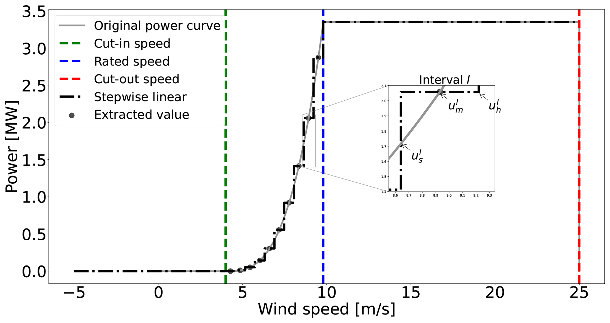
Figure 1 Piecewise constant approximation of a wind turbine power curve through sampling with m=10 intervals between the cut-in and rated wind speeds.

Let binary state variables ${\mathit{\eta }}_{ijk}^l\in \mathit{\{}\mathrm{0},\mathrm{1}\mathit{\}}$ for $l=\mathrm{1},\mathrm{\dots },m+\mathrm{2}$ be defined with the interpretation

$$\begin{array}{}\text{(17)}& {\mathit{\eta }}_{ijk}^l=\left\{\begin{array}{ll}\mathrm{1}& \text{if }{u}_s^l\le u_{ijk}\le u_h^l\text{ and }\\ \mathrm{0}& \text{otherwise;}\end{array}\right.\end{array}$$

i.e., these variables indicate which of the wind speed intervals l of the power curve approximation for WT i operates at wind direction j and wind speed k.

With all the variables of the model – activation variables ξ, continuous state variables u, and binary state variables η – introduced, the formulation in Eq. (18) is as follows:

$$\begin{array}{}\text{(18a)}& {\displaystyle }\underset{\mathit{\xi },\mathit{\eta },u}{\text{maximize }}\mathrm{8760}\sum _{i=\mathrm{1}}^N\sum _{j,k}\sum _{l=\mathrm{1}}^{m+\mathrm{2}}{w}_{jk}{\mathit{\eta }}_{ijk}^{l}p\left(u_m^l\right),\text{(18b)}& {\displaystyle }\text{subject to }{\mathit{\xi }}_i+{\mathit{\xi }}_q\le \mathrm{1}i,q\in {\mathbf{N}}_i,\text{(18c)}& {\displaystyle }{n}^{min}\le \sum _{i=\mathrm{1}}^N{\mathit{\xi }}_j\le n^{max},\text{(18d)}& {\displaystyle }\sum _{l=\mathrm{1}}^{m+\mathrm{2}}{\mathit{\eta }}_{ijk}^l{u}_s^l\le u_{ijk}\le \sum _{l=\mathrm{1}}^{m+\mathrm{2}}{\mathit{\eta }}_{ijk}^l{u}_h^l(i,j,k),\text{(18e)}& {\displaystyle }\sum _{l=\mathrm{1}}^{m+\mathrm{2}}{\mathit{\eta }}_{ijk}^l=\mathrm{1}(i,j,k),\text{(18f)}& {\displaystyle }{u}_{ijk}=u_{\mathrm{\infty }}^k\left({\mathit{\xi }}_i-\sum _{\mathrm{\ell }\in {\mathbf{U}}_i^{{\mathit{\theta }}^j}}{\mathit{\xi }}_{\mathrm{\ell }}{\mathit{\delta }}_{i\mathrm{\ell }}\left({\mathit{\theta }}^j,u_{\mathrm{\infty }}^k\right)\right)(i,j,k),\text{(18g)}& {\displaystyle }\mathit{\xi },\mathit{\eta }\in \mathit{\{}\mathrm{0},\mathrm{1}\mathit{\}}u\in \mathbb{R}.\end{array}$$

This program collects the AEP objective function, the constraints of a generalized version of the WFLO problem, and the variables' domain definition. The objective function in Eq. (18a) is an approximation of the AEP computation presented in Eq. (9). Equation (18b) models the minimum distance constraints as explained in the introduction of Sect. 3. If binary variable ξ_i is active, then all candidate points closer than d^min should be excluded, i.e., set to 0. If binary variable ξ_i is inactive, then the other candidates are still eligible. The definition of set N_i is provided in Eq. (11). Equation (18c) models the situation in which the designer requires at least n^min and at most n^max WTs to be located in the domain. Note that for the classic problem definition $n^{min}=n^{max}$=n_T, Eq. (18d) connects state variables u and η as explained in Eq. (17), while Eq. (18e) forces one operation case to be active for each WT candidate at each wind direction and speed. The last constraint in Eq. (18f) is for the wake velocity deficit and wake superposition modeling to calculate wind speed for each candidate location at each wind direction and inflow speed $u_{\mathrm{\infty }}^k$. The presented model supports a conservative velocity deficit approach (Eq. 3) with a linear superposition (Eq. 6). The definition of set ${\mathbf{U}}_i^{{\mathit{\theta }}^j}$ is provided in Eq. (5). Note that an extension, consisting in creating extra continuous state variables and associated constraints, could allow for considering the more realistic approach in Eq. (4). It is still unknown if the root sum squares model of Eq. (7) could be implemented in the framework of MILP. Finally, Eq. (18g) defines the domain of the required variables. A value for uⁱⁿⁱ of u^cut-out is set up.

3.2 Power-curve-free model

Although the formulation of Sect. 3.1 represents the physics ruling the problem to a very large extent, it has a considerable number of variables and constraints that may hinder the capacity to tackle larger problems. The model presented in this section neglects the power curve and AEP calculation and aims at simplifying the power-curve-based version.

The power-curve-free model introduces a strategy to account for the combination of Eqs. (3) and (7) to calculate velocities, since the case studies from IEA Wind Task 37 follow this methodology for AEP computation. It would be possible though to consider the linear superposition model if necessary. However, the power-curve-free model does not support the application of Eq. (4).

Combining Eqs. (3) and (7) and extending the summation range in Eq. (7) to all candidate locations, the sum of wind speeds in the farm U can be modeled as

$$\begin{array}{}\text{(19)}& U=\sum _{i=\mathrm{1}}^N\sum _{j,k}{w}_{jk}{u}_{\mathrm{\infty }}^k{\mathit{\xi }}_i-\sum _{i=\mathrm{1}}^N\sum _{j,k}{w}_{jk}{u}_{\mathrm{\infty }}^k\sqrt{\sum _{\mathrm{\ell }=\mathrm{1}}^N\left({\mathit{\delta }}_{i\mathrm{\ell }}\right({\mathit{\theta }}^j,u_{\mathrm{\infty }}^k){)}^{\mathrm{2}}{z}_{i\mathrm{\ell }}},\end{array}$$

where new binary variables z_iℓ are introduced. Variable z_iℓ is equal to 1 if both WTs i and ℓ are active (i.e., if ${\mathit{\xi }}_i={\mathit{\xi }}_{\mathrm{\ell }}=\mathrm{1}$) and 0 otherwise. Nevertheless, the previous expression is not linear for variable z_iℓ due to the presence of the square root in each total relative velocity deficit term. By removing the square roots, the following expression is obtained:

$$\begin{array}{}\text{(20)}& \begin{array}{rl}\stackrel{\mathrm{̃}}{U}& =\stackrel{\text{total inflow wind speed}}{\overbrace{\sum _{i=\mathrm{1}}^N\sum _{j,k}{w}_{jk}{u}_{\mathrm{\infty }}^k{\mathit{\xi }}_i}}\\ & -\stackrel{\text{total wind speed deficit proxy}}{\overbrace{\sum _{i=\mathrm{1}}^N\sum _{\mathrm{\ell }=\mathrm{1}}^N\sum _{j,k}{w}_{jk}{u}_{\mathrm{\infty }}^k\left({\mathit{\delta }}_{i\mathrm{\ell }}\right({\mathit{\theta }}^j,u_{\mathrm{\infty }}^k){)}^{\mathrm{2}}{z}_{i\mathrm{\ell }}}},\end{array}\end{array}$$

where the arguments of the square roots in Eq. (19) define a function closely related to the full root-squared expression. This linearization approach is similar to the one proposed by Turner et al. (2014). Let the preprocessed coefficient in front of z_iℓ be

$$\begin{array}{}\text{(21)}& b_{i\mathrm{\ell }}=\sum _{j,k}{w}_{jk}{u}_{\mathrm{\infty }}^k\left({\mathit{\delta }}_{i\mathrm{\ell }}\right({\mathit{\theta }}^j,u_{\mathrm{\infty }}^k){)}^{\mathrm{2}},\end{array}$$

and combining Eq. (20) and Eq. (21) results in

$$\begin{array}{}\text{(22)}& \stackrel{\mathrm{̃}}{U}=\stackrel{\text{total inflow wind speed}}{\overbrace{\sum _{i=\mathrm{1}}^N\sum _{j,k}{w}_{jk}{u}_{\mathrm{\infty }}^k{\mathit{\xi }}_i}}-\stackrel{\text{total wind speed deficit proxy}}{\overbrace{\sum _{i=\mathrm{1}}^N\sum _{\mathrm{\ell }>i}^N(b_{i\mathrm{\ell }}+b_{\mathrm{\ell }i})z_{i\mathrm{\ell }}}},\end{array}$$

which defines the objective function of the power-curve-free model. In comparison to the objective function in Eq. (18a), no power curve or continuous state variables are required.

Nonetheless, the presence of variables z_iℓ can be troublesome. For the complete model, in addition to having these variables of a combinatorial nature, constraints of the same kind must be incorporated: $z_{ij}\ge {\mathit{\xi }}_i+{\mathit{\xi }}_j-\mathrm{1}$, z_ij≤ξ_i, $z_{ij}\le {\mathit{\xi }}_j,z_{ij}\ge \mathrm{0}$. Experimental results show the heavy computational burden incurred when solving this formulation, impacting the ability of solving large-scale problems (Fischetti et al., 2016). To circumvent this, a big-M trick is incorporated (Wolsey, 2020), resulting in an exactly equivalent model, as reflected in the formulation of Eq. (23).

The new objective function in Eq. (23a) modifies the component linked to the total wind speed deficit proxy by creating variables τ_i; this variable means the total wind speed deficit proxy for WT in candidate location i. Equation (23b) defines τ_i as follows: if a WT candidate location is inactive as ξ_i=0, then there is no deficit at this location; therefore τ_i=0 because $M_i={\sum }_{\mathrm{\ell }=\mathrm{1}:i\ne \mathrm{\ell }}^N{b}_{i\mathrm{\ell }}$ and because of the minimization nature of the problem for wind speed deficits. Oppositely, if ξ_i=1, then τ_i is forced to be equal to ${\sum }_{\mathrm{\ell }=\mathrm{1}:i\ne \mathrm{\ell }}^N{\mathit{\xi }}_{\mathrm{\ell }}{b}_{i\mathrm{\ell }}$. The next two equations are the same as those already presented in Sect. 3.1 for the number of active WTs and minimum distance constraints. Finally, Eq. (23e) defines the domain of the required variables as follows:

$$\begin{array}{}\text{(23a)}& {\displaystyle }\underset{\mathit{\xi },\mathit{\tau }}{\text{maximize}}\stackrel{\text{total inflow wind speed}}{\overbrace{\sum _{i=\mathrm{1}}^N\sum _{j,k}{w}_{jk}{u}_{\mathrm{\infty }}^k{\mathit{\xi }}_i}}-\stackrel{\text{total wind speed deficit proxy}}{\overbrace{\sum _{i=\mathrm{1}}^N{\mathit{\tau }}_i,}}\text{(23b)}& {\displaystyle }\text{subject to }{\mathit{\tau }}_i\ge \sum _{\mathrm{\ell }=\mathrm{1}:i\ne \mathrm{\ell }}^N{\mathit{\xi }}_{\mathrm{\ell }}{b}_{i\mathrm{\ell }}+({\mathit{\xi }}_i-\mathrm{1})M_{i}i,\text{(23c)}& {\displaystyle }{n}^{min}\le \sum _{i=\mathrm{1}}^N{\mathit{\xi }}_i\le n^{max},\text{(23d)}& {\displaystyle }{\mathit{\xi }}_i+{\mathit{\xi }}_q\le \mathrm{1}i,q\in {\mathbf{N}}_i,\text{(23e)}& {\displaystyle }\mathit{\xi }\in \mathit{\{}\mathrm{0},\mathrm{1}\mathit{\}}\mathit{\tau }\in \mathbb{R}:\mathit{\tau }\ge \mathrm{0}.\end{array}$$

Note that for the classic problem definition $n^{min}=n^{max}$=n_T, the first part of the objective function becomes

$$\begin{array}{rl}\sum _{i=\mathrm{1}}^N\sum _{j,k}{w}_{jk}{u}_{\mathrm{\infty }}^k{\mathit{\xi }}_i& =\sum _{j,k}{w}_{jk}{u}_{\mathrm{\infty }}^k\sum _{i=\mathrm{1}}^N{\mathit{\xi }}_i\\ & =\sum _{j,k}{w}_{jk}{u}_{\mathrm{\infty }}^k{n}_{\text{T}}=\text{constant}.\end{array}$$

For this situation, the objective function is thus equivalent to

$$\begin{array}{}\text{(24)}& \underset{\mathit{\xi },\mathit{\tau }}{\text{minimize}}\sum _{i=\mathrm{1}}^N{\mathit{\tau }}_i.\end{array}$$

This proxy objective function is very useful for formulating the program in the MILP category. The work by LoCascio et al. (2022) focuses on a different formulation (likely more accurate analytically than the one presented here) that is non-linear but gradient friendly and is hence useful for continuous gradient-based optimization.

Compared to Turner et al. (2014), the MILP program (Eq. 23) with an objective replaced by Eq. (24) linearizes the complexity of its largest set of constraints and variables from N² to N in Eqs. (23b) and (23e). Furthermore, the constraints in Eq. (23d), which can lead to infeasible points, are not neglected as by Turner et al. (2014).

4 Neighborhood search heuristic

For addressing large-scale problems, a heuristic wrapping the MILP formulations given in Sect. 3 is introduced. It is based on the neighborhood search and local-branching theory (Fischetti and Lodi, 2003). The algorithm solves a sequence of MILPs, with different candidate numbers N and/or neighborhood search sizes K, taking advantage of robust and efficient implementations of branch-and-cut methods for MILP. The heuristic relies on the observation that for a fixed layout described by $\mathit{\xi }\in \mathit{\{}\mathrm{0},\mathrm{1}{\mathit{\}}}^N$, the other state variables are straightforward to determine. This observation is valid for all problem formulations presented in Sect. 3. Given $\mathit{\xi }\in \mathit{\{}\mathrm{0},\mathrm{1}{\mathit{\}}}^N$, for the power-curve-based model, the value of continuous state variables u can be found through classical wake analysis, and the binary state variables η are directly determined by inspection of the velocities. Similarly, for the power-curve-free model, the τ variables are trivially computed. The pseudo-code of the neighborhood search heuristic (NSH) is described in detail in Algorithm 1.

The first three lines are the main inputs of the algorithm: the candidate set C, the time set T, and the neighborhood size set V. The first set contains the sizes N of the meshes to be considered, the second one is the maximum computing time T for the MILP solver for each size N, and the last one is for the search size defined as the maximum number of changes K allowed for the incumbent. If the incumbent is improved, then the candidate set C and neighborhood size K are kept; otherwise at least one of them is increased. The first step (line 5) is to obtain an initial incumbent binary variables, with the set ξ storing the acquired value (0 or 1) for each variable ${\mathit{\xi }}_i:i\le N$. The incumbent has an objective value of o_b calculated after the true objective function. The true objective function refers to the real equation that represents the ultimate aim to be optimized. For example, if this is the AEP, then it is the product of the power calculation process, applying the considered wake and superposition models and the original power curve, and not the objective function of the implemented formulation, as in Eq. (18a), which is always an approximation.

The next step is to start the iterative process in line 6. Values for N, T, and K are fetched in line 7, followed by the formulation of the MILP model for candidates N accounting for the active locations in ξ. The Hamming distance (see, e.g., Fischetti and Lodi, 2003), centered around incumbent point ξ, is added to the optimization model in line 9; this constraint reduces the search space as the number of changes in ξ are limited to K. The complete model is sent to the MILP solver with ξ as a warm starter, which is stopped when it reaches either optimality or assigned maximum computing time T.

Algorithm 1 Neighborhood search heuristic (NSH) algorithm. Optimization: op.

1:

$\mathbf{C}\leftarrow \left\{N_{\mathit{1}},\mathrm{\cdots },N_C\right\},N\in \mathbf{C}$ {Input candidate set}

2:

$\mathbf{T}\leftarrow \left\{T_{\mathit{1}},\mathrm{\cdots },T_C\right\},T\in \mathbf{T}$ {Input time set}

3:

$\mathbf{V}\leftarrow \left\{K_{\mathit{1}},\mathrm{\cdots },K_V\right\},K\in \mathbf{V}$ {Input neighborhood size set}

4:

countern←1 counterv←1

5:

Obtain initial incumbent of activation binary variables for WTs ξ with objective value o_b

6:

for $(\mathit{\kappa }=\mathit{1}:\mathit{1}:{\mathit{\kappa }}_{\text{max}})$ do

7:

N←C[countern] T←T[countern] K←V[counterv]

8:

Formulate optimization model with N candidates (including the incumbent), from either Sect. 3.1 or Sect. 3.2

9:

Add Hamming distance constraint centered around the incumbent ξ, ${\sum }_{i:{\mathit{\xi }}_i=\mathrm{0}}{\mathit{\xi }}_i+{\sum }_{i:{\mathit{\xi }}_i=\mathrm{1}}(\mathrm{1}-{\mathit{\xi }}_i)\le K$

10:

Solve op. model from algorithm lines 8 to 9 until optimality or computing time T with ξ as a warm starter

11:

Get the solution pool S, where $\widehat{\mathit{\xi }}\in \mathbf{S}$ represents the activation binary variables for WTs of an individual point

12:

Apply true objective function over each point $\widehat{\mathit{\xi }}\in \mathbf{S}$ and obtain objective value set O

13:

Compute $o_t\leftarrow max\mathbf{O}$ and $i_t\leftarrow \arg max\mathbf{O}$

14:

if o_t>o_b then

15:

o_b←o_t

16:

ξ←S[i_t]

17:

else

18:

$\mathit{counterv}\leftarrow \mathit{counterv}+\mathit{1}$

19:

end if

20:

if $\mathit{counterv}=\left|\mathbf{V}\right|+\mathit{1}$ then

21:

counterv←1 $\mathit{countern}\leftarrow \mathit{countern}+\mathit{1}$

22:

end if

23:

if $\mathit{countern}=\left|\mathbf{C}\right|+\mathit{1}$ then

24:

Break

25:

end if

26:

end for

After solver termination, solution pool S is retrieved in line 11. The solution pool contains all the feasible layouts obtained in iteration κ from the MILP solver. These points are a result of a linear programming relaxation or from applying heuristics in a given node, such as relaxation-induced search, polishing, and a feasibility pump (IBM, 2022). It is very important to emphasize the aim of getting the whole pool instead of the best point. This is done because of the imperfect correspondence between the true objective function and the objective function of the applied MILP model. For example, a solution which has a worse objective value may actually have a better AEP based on the real model. One of the advantages of the NSH compared to the DEBO algorithm by Thomas et al. (2023) is the reduced number of AEP evaluations. In iteration κ, only $\left|\mathbf{S}\right|$ evaluations are required. Likewise, many of the other expensive calculations are done in a preprocessing stage. The whole pool of solutions is examined, and the best solution indexed by i_t with an AEP of o_t is obtained in line 13. If o_t is actually greater than o_b, then the whole algorithm is re-centered around the new ξ (lines 14 to 16), and in the next iteration κ, the same values of N and K are maintained. Otherwise, the next value of K is taken (line 18), unless the set has been exhausted. In this case, the next candidate size N is considered given by countern, restarting the neighborhood set counter counterv to 1 (lines 20 to 22). The NSH algorithm is terminated when all candidate sets C have been processed (line 23 to 25). Another difference between the NSH and the DEBO algorithm is that the latter only changes the position of a single WT in a given iteration, while the former considers simultaneous modifications of several WT positions.

5 Computational experiments

For a transparent benchmark of the proposed methods, the open-access case studies from IEA Wind Task 37 in Baker et al. (2019) are used for comparison. IEA Wind Task 37 cases consider circular project areas with three different radii (1300, 2000, and 3000 m) and numbers of WTs (16, 36, and 64) (n_T). Thus, Case I has a radius of 1300 m and n_T=16 WTs, whereas Case II has a radius of 2000 m and n_T=36, and Case III has a radius of 3000 m and n_T=64, correspondingly.

The results of the statistical correlation between the proxy function given by the argument in Eq. (24) and AEP of the problem definition of Baker et al. (2019) are presented in Sect. 5.1 for each case. The performance of the proposed models in the case studies is shown in Sect. 5.2 (Case I), 5.3 (Case II), and 5.4 (Case III). The power-curve-free model of Eq. (23) is implemented with Eq. (24) as an objective function in these three sections. The true objective function in the NSH of Algorithm 1 for these cases is the AEP of the problem definition. Finally, to prove the capabilities of power-curve-based model of Eq. (18), Sect. 5.5 displays results after applying this formulation with a modified objective function to express a metric similar to the NPV.

The main parameters of the wake model in Sect. 2.1 are fixed to $C_{\text{T}}=\mathrm{8}/\mathrm{9}$ and k_y=0.0324555, according to Baker et al. (2019). The wind resource is modeled using a wind rose approach, where the wind resource is binned in J directions, and for a specific direction j (θ^j), wind speeds are discretized in Υ sectors. For the case studies, the wind rose is composed of 16 directions and a single wind speed k of 9.8 ms⁻¹, shown in Fig. 2. The power curve from Eq. (8) modeling the IEA Wind Task 37 3.35 MW reference turbine (with diameter of D=130 m) is used in the case studies, ensuring replicability of results (IEA Wind Task 37, 2019; Baker et al., 2019). The main parameters are p^rated=3.35 MW, u^rated=9.8 ms⁻¹, u^cut-in=4 ms⁻¹, and u^cut-out=25 ms⁻¹ and are plotted in Fig. 1. The parameter d^min is set to 2 D.

The experiments in Sect. 5.2, 5.3, and 5.4 have been carried out on an Intel Core i7-6600U CPU running at 2.80 GHz with four logical processors and 16 GB of RAM. For the experiment in Sect. 5.5, more powerful equipment is used: an Intel Xeon Gold 6226R CPU running at 2.90 GHz with 32 virtual cores and 640 GB of RAM (DTU Computing Center, 2022).

The selected MILP solver is the commercial branch-and-cut algorithm implemented in IBM ILOG CPLEX Optimization Studio V20.1 (IBM, 2022). Apart from the number of threads and time limit settings, a few other parameters are also changed from their default values. One is the parameter returning high-quality feasible solutions early in the process, for which CPX_MIPEMPHASIS_HEURISTIC is activated. The intention is to generate more feasible layouts, which is important for the neighborhood search algorithm. Additionally, strong branching is used for variable selection given the large size of the models (CPX_VARSEL_STRONG is selected). The intention is to reduce the size of the search tree and thus the memory requirements compared to default settings.

The number N and positions p_i for i≤N of the candidate locations are of course very important parameters for the discrete modeling techniques. A customized automatic strategy based on independently sampling the boundary and interior area of the circular domain F has been employed. An example of the sampling strategy for these particular case studies giving N=467 is illustrated in Fig. 3.

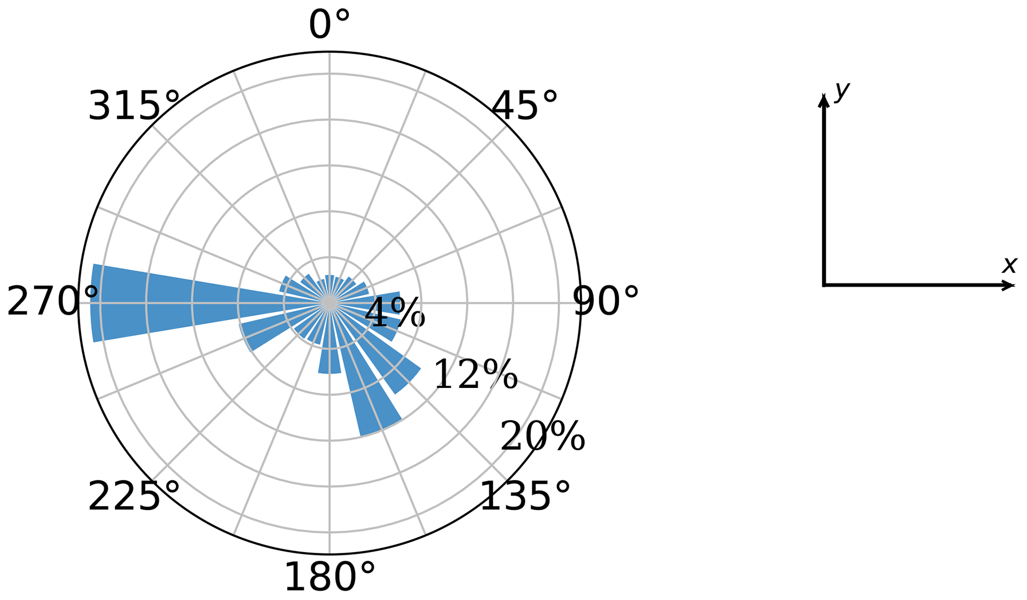
Figure 2 Wind rose used in the computational experiments. Taken from an open-access source (IEA Wind Task 37, 2019).

Figure 3 Example of generation of WT candidate locations N.

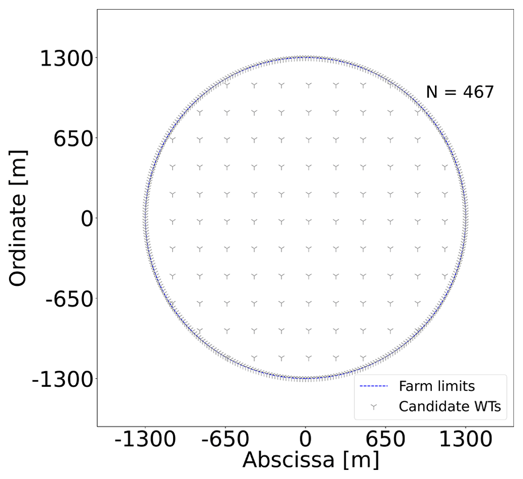
In Fig. 3, the boundary of the circular shape is densely sampled, as a candidate point is defined every natural angle from 0 to 359^∘; i.e., 360 candidate points are provided, since it is intuitively expected that a good portion of the WTs will be placed in the boundaries to decrease wake losses. For the interior, a set of finite parallel line segments are generated, and the candidates points are then taken along those segments. In the example of Fig. 3, the slope of the line segments is 0, and the distance between points and lines is equal to 1.7 D.

5.1 Correlations

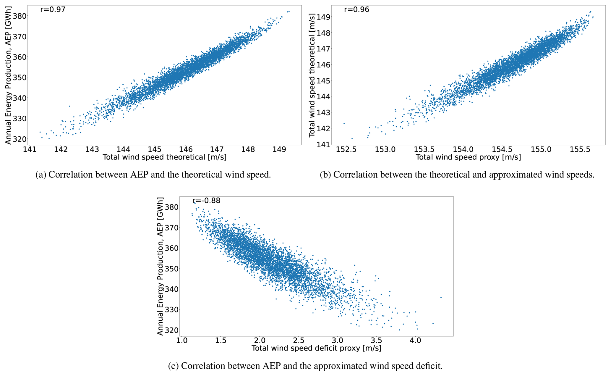
To validate the approach modeled by the MILP formulation of Eq. (23) (i.e., the power-curve-free model), 5000 random feasible WT layouts are created. For each of them, the AEP of Baker et al. (2019), the total theoretical wind speed U, given by Eq. (19); the total wind speed proxy $\stackrel{\mathrm{̃}}{U}$, defined by Eq. (22); and total wind speed deficit proxy ${\sum }_{i=\mathrm{1}}^N{\mathit{\tau }}_i$, an argument of Eq. (24), are calculated. Although the random way of generating the layouts is biased against high-quality points, the general trend is the point of interest for assessing whether it makes sense to implement the linear proxy objective ${\sum }_{i=\mathrm{1}}^N{\mathit{\tau }}_i$ when optimizing the AEP.

In all cases Pearson product-moment linear correlation coefficients from Pearson (1895) are used to extract information from the data and collected in Table 1 for all pairs. This coefficient illustrates the degree to which the movement of pairs of variables is associated in a linear fashion. The correlation plots of Fig. 4 present the graphical representation of the relations for Case I.

The correlation between the AEP and the total theoretical wind speed is shown in Fig. 4a for Case I. The main observation is the very strong linear relation between these two variables as illustrated by the correlation coefficient of 0.97. Interestingly, this reflects the rather low influence of the WT power curve in obtaining high-quality feasible points. The relation between U and $\stackrel{\mathrm{̃}}{U}$ is represented in Fig. 4b, resulting in an almost identical linear connection between them, as in the previous graph. When one compares the AEP vs. ${\sum }_{i=\mathrm{1}}^N{\mathit{\tau }}_i$, however, it is noticeable that the Pearson coefficient decreases to −0.88. There is a wider area in the body of points that causes this behavior. Note that in contrast to the previous two figures, there is a negative correlation because the comparison is done in terms of the wind speed deficit instead of the total wind speed. In spite of this deterioration, the linear correlation is still considered quite strong. These results motivate the approach where the minimization of a proxy total wind speed deficit can lead to high-quality AEP solutions. The NSH of Algorithm 1 helps in correcting the imperfect correspondence between these two variables during the optimization routine as reflected in Sect. 4.

Table 1 Pearson product-moment linear correlation coefficients for all case studies.

Figure 4 Correlation plots for 5000 randomly generated wind turbine layouts for Case I.

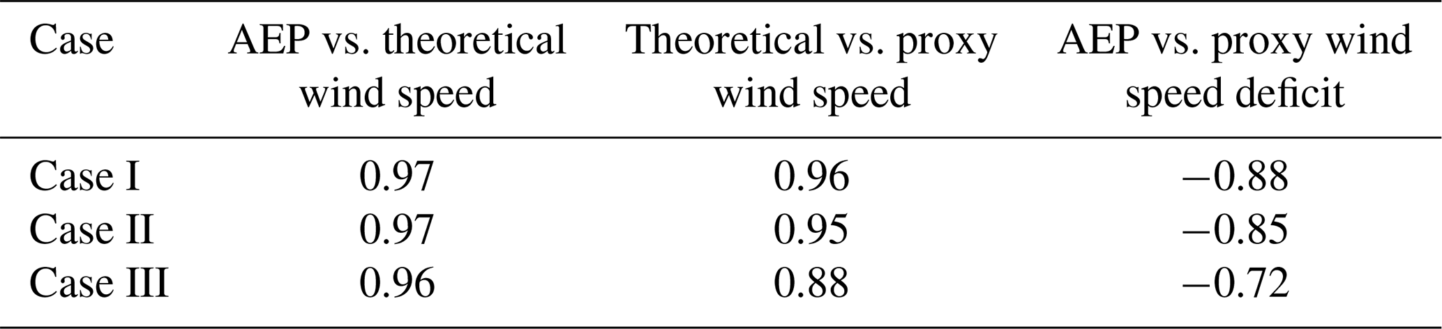
The general trends of the correlation plots for Case II are very similar. Correlations between the AEP and the total theoretical wind speed (0.97) and the total theoretical wind speed and the total wind speed proxy (0.95) are still very strong. Nonetheless, there is a slight decrease between the AEP and the total wind speed proxy (down to −0.85 from −0.88 previously), as the spread for middle-velocity values is larger. The linear relation is deemed satisfactory enough to carry on with the application of the model of Eq. (23) with the objective function in Eq. (24).

The very strong linear relation between the AEP and the total theoretical wind speed (0.96) is also observed for Case III, prompting a very interesting conclusion. Although almost all research in the WFLO space focuses strictly on power modeling (which brings a great deal of complexity due to the non-linear and non-differentiable properties of the WT power curve), using an exact model for determining the total wind speed as an objective function alleviates the computational complexity while finding high-quality solutions in terms of the AEP. However, one should note that deterioration in the correlation still exists, potentially leading to lower-quality results.

Likewise, correlations stemming from the proxy to calculate the total wind speed deficit are lower in Case III. This is the case for both with the total theoretical wind speed (0.88) and the AEP (−0.72). Keep in mind that the reason to formulate such an approximation is to fit it into the context of integer programming to leverage theory and state-of-the-art algorithms from this mature field. However, the price one pays to do so is losing fidelity in representing the real (true) target to optimize. The deterioration in the correlation of these pairs of variables may also suggest the need to resort to the power-curve-based model for some applications. Whether the price is too high or not is reflected in the reachable solution quality. Section 5.2, 5.3, and 5.4 present the optimization results for the cases of a fixed number of WTs that will ultimately help to elucidate a final evaluation regarding the adopted modeling technique.

5.2 Case I: 16 WTs

This case has a round shape with a radius of 1300 m and n_T=16 WTs. The evolution of two of the proposed optimization frameworks is given in Fig. 5 (clock time given in the abscissa). The green line of the full model is obtained after solving the model of Eq. (23) with an objective function as in Eq. (24) for N=1014 without implementing the NSH. It represents the incumbent solution in terms of the AEP (not the total wind speed deficit proxy) obtained by postprocessing the CPLEX's log. The blue line results from applying the NSH with the model of Eq. (23) plus the objective of Eq. (24) and the AEP as the true objective function of Algorithm 1. The main inputs are $\mathbf{C}=\left\{\mathrm{467},\mathrm{590},\mathrm{1014}\right\}$ (set of candidate locations), $\mathbf{T}=\left\{\mathrm{1},\mathrm{1.5},\mathrm{2}\right\}$ h (set of maximum computing times for each candidate location), and $\mathbf{V}=\left\{\mathrm{2},\mathrm{4},\mathrm{6},\mathrm{16}\right\}$ (set of neighborhood search sizes) (see Sect. 4). These inputs are tuned after evaluating the performance of the method using different values. In general, the first two elements of C consist of moderately big values, relatively close to each other, while the last element is sizably greater in the search of the best possible solution. Each element N∈C has an associated computing time T. Finally, the first elements of V are relatively low values that favor termination of the solver due to optimality, and then they start increasing to refine the search. The red line is for establishing a reference of the AEP value; this comes from the best performing method in the survey of IEA Wind Task 37 of Baker et al. (2019), the SNOPT plus the wake expansion continuity (WEC) (Thomas and Ning, 2018; Thomas et al., 2022). Time evolution for the SNOPT + WEC is not reflected in this graph, as this information is unavailable. Results for the benchmark against a test bed of different algorithms are available in Table 2.

The results of the NSH computing time in Fig. 5 do not reflect the instant where the incumbent is found but rather the time progress of this algorithm, which is dependent on the execution of the MILP solver at each iteration. Table A1 contains information about the values of N, K, and T and the termination criterion of the solver after each iteration κ of the NSH of Algorithm 1 (beginning from point 2, where κ=1). This means that, in iterations where the termination criterion is time (and not optimality), one could fine-tune T for an earlier stop, shortening the total time. This is particularly more relevant in cases where internal heuristics of the solver are activated at the root node of the search tree, coming up with the largest portion of solutions very early in the process. Consequently, the total computing time, for all cases, is conservative and should be taken as an approximated reference.

The initial layout (point 1), labeled in Fig. 6a, is set up by arbitrarily by picking up candidate locations around the circular boundary; this layout has an AEP of 387 GW h. From now on, the presented percentages are calculated with respect to the last-commented AEP improvement. Between points 2 and 7, where N=467 and K=2, the models are solved to optimality (gap of 0 %), and the solution is improved by 2.92 % in only 56 s. After a short plateau, the solution is markedly refined by 2.96 % from point 10 to 13 by performing a search of the domain with K=16 and restarting the model every 1 h with a new warm start.

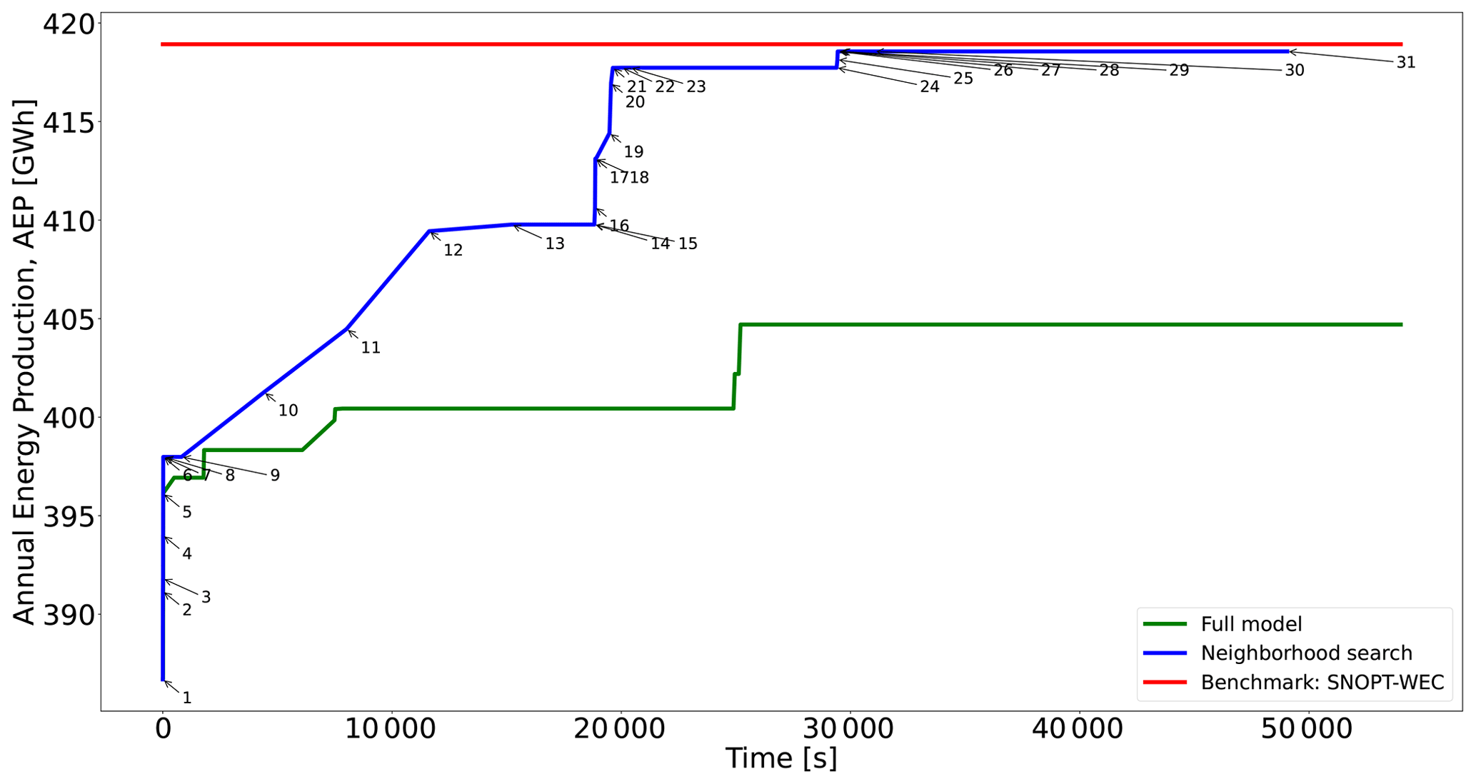
Figure 5 Performance of two different optimization approaches for Case I and comparison with existing best benchmark results. See Table A1 for detailed information about each numbered point in the blue curve.

The next considerable jump happens for N=590 and $\mathrm{2}\le K\le \mathrm{6}$ after around 20 min, elevating the AEP by 1.94 %. After, again, a plateau without improvements, when N reaches its maximum value of 1014, the solution is maximized to the final value of 418 GW h during the lowest values of K. For this particular instance, the greatest value of K=16 is exploited for the lowest number of candidate points N, where the largest improvement comes up.

The benefit of the proposed neighborhood search strategy is shown in Fig. 5. Solving the full model is significantly slower, actually leading to a worse solution (3.31 % lower). The capacity of the NSH to iterate over different values of candidate points N and search sizes K brings along improvements in terms of not only the solution time and solution quality but also the use of fewer computational resources as the RAM memory generally scales faster when solving the single model.

The initial and final solution layouts for this case study are illustrated in Fig. 6. The importance of finely sampling the boundaries of the available area is evident in Fig. 6b because 7 out of the 16 WTs are placed in that subdomain.

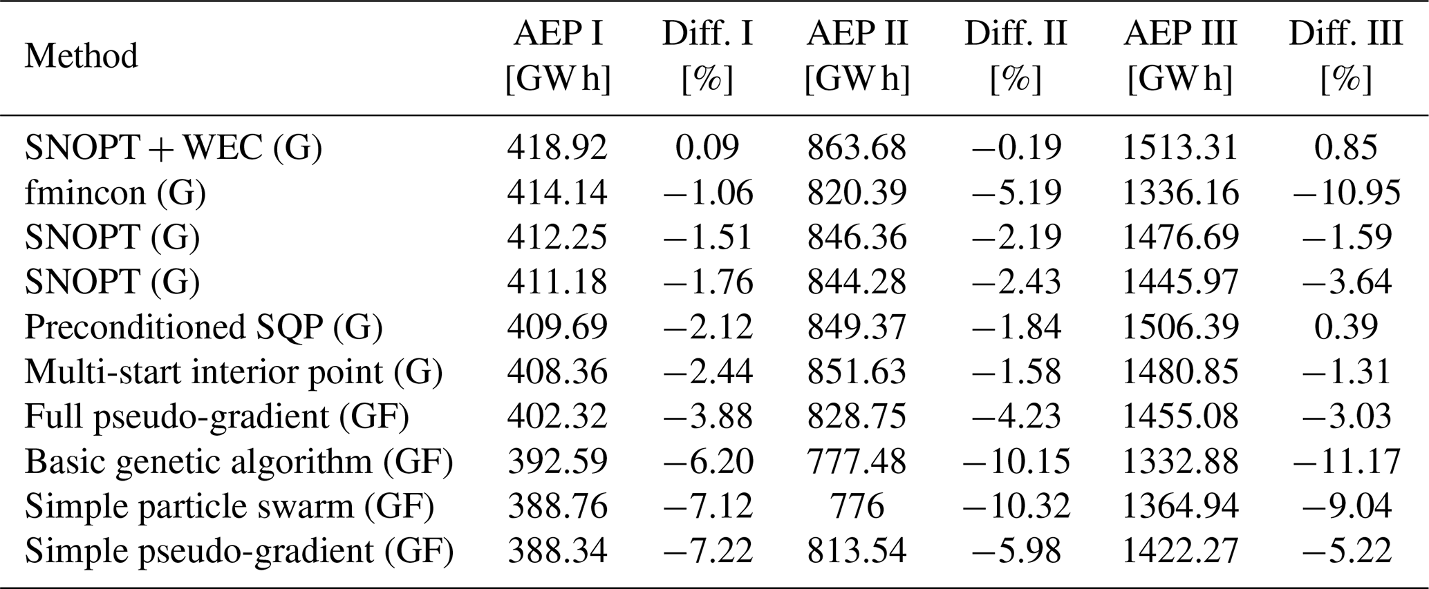
Finally, Table 2 compares the proposed method to a large number of different approaches from the IEA Wind Task 37 reference study (Baker et al., 2019). The results for all case studies are presented, where I, II, and III make reference to cases from this section, Sect. 5.3, and Sect. 5.4, respectively.

The third column of Table 2 reports the difference in the AEP with respect to the proposed method for the smallest case study. The resulting AEP is better than almost all the other alternatives, except the SNOPT + WEC, where a nearly identical objective value is achieved. When directly comparing to typical metaheuristics (genetic algorithms, particle swarm optimization, etc.), which do not use explicit gradients information, the presented method seems to perform well, being capable of determining a similar layout quality in less than 2 h, which is usually a competitive amount of time compared to these kinds of population-based algorithms. In a broader context, beyond the presented numerical comparisons, discrete optimization approaches, such as the MILP ones presented in this paper, could be formulated to cope with problem definitions with required functionalities that in theory continuous optimization methods can not support (or at least for which the implementation becomes strenuous).

Figure 6 Generated wind farm layouts for benchmark Case I with 16 turbines.

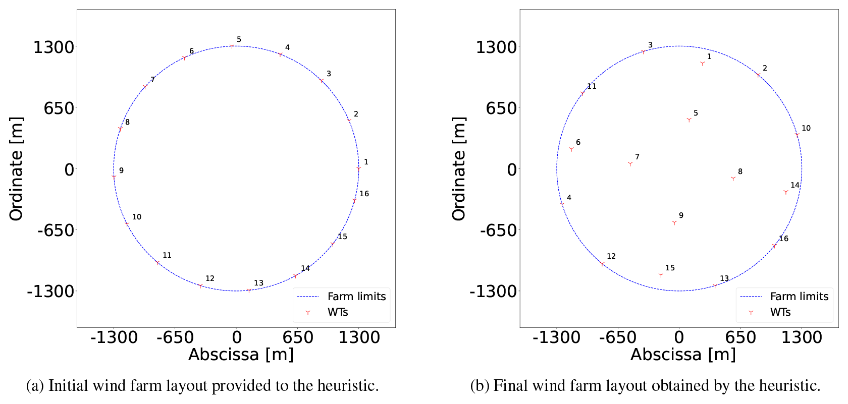
Table 2 Results for all three benchmark cases from other algorithms (G, gradient-based; GF, gradient-free) obtained while allowing for WT locations to vary continuously. Values reproduced from Baker et al. (2019). The difference (Diff.) column shows how the proposed heuristic with the power-curve-free model performs in comparison. Negative percentages mean that the proposed method performs better than the corresponding algorithm.

The power-curve-based model of Eq. (18) within the NSH using the same AEP formulation as true objective function provides a solution 1.18% lower in objective value after around 36 h using the computer system with 32 virtual cores. Although the quality of the layout is very close to the one schematized in Fig. 6b, the use of more computationally powerful resources favors implementing the power-curve-free model for problems with a fixed number of WTs. Therefore, Sect. 5.3 and 5.4 present only the results reached after the application of the power-curve-free model embedded into the NSH.

5.3 Case II: 36 WTs

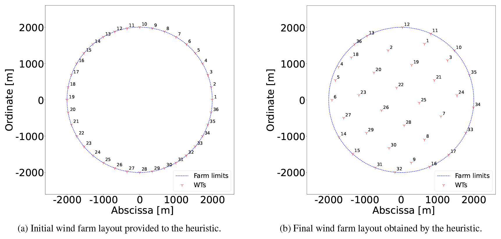
This case has a round shape with a radius of 2000 m and n_T=36 WTs. The evolution of the proposed methods and the initial and final WT layouts are plotted in Figs. 7 and 8, respectively. Table B1 displays the data linked to each point of Fig. 7. The main inputs are $\mathbf{C}=\left\{\mathrm{477},\mathrm{684},\mathrm{1907}\right\}$, $\mathbf{T}=\left\{\mathrm{1},\mathrm{1.5},\mathrm{2}\right\}$ h, and $\mathbf{V}=\left\{\mathrm{2},\mathrm{4},\mathrm{8},\mathrm{16},\mathrm{36}\right\}$. The blue line (model of Eq. 23 with an objective function of Eq. 24 plus the NSH of Algorithm 1) clearly has three sectors stemming from each value of N∈C. The initial WT layout (Fig. 8a) – also determined by choosing roughly equidistant candidate locations in the boundary – has an AEP of 796 GW h. As for Case I, improvement percentages are calculated using the last-commented step as the baseline. After seven NSH iterations (point 8) in 41 s, the incumbent is improved by 1.84%, when N=477 and $\mathrm{2}\le K\le \mathrm{4}$, being able to solve each model instantiation to optimality.

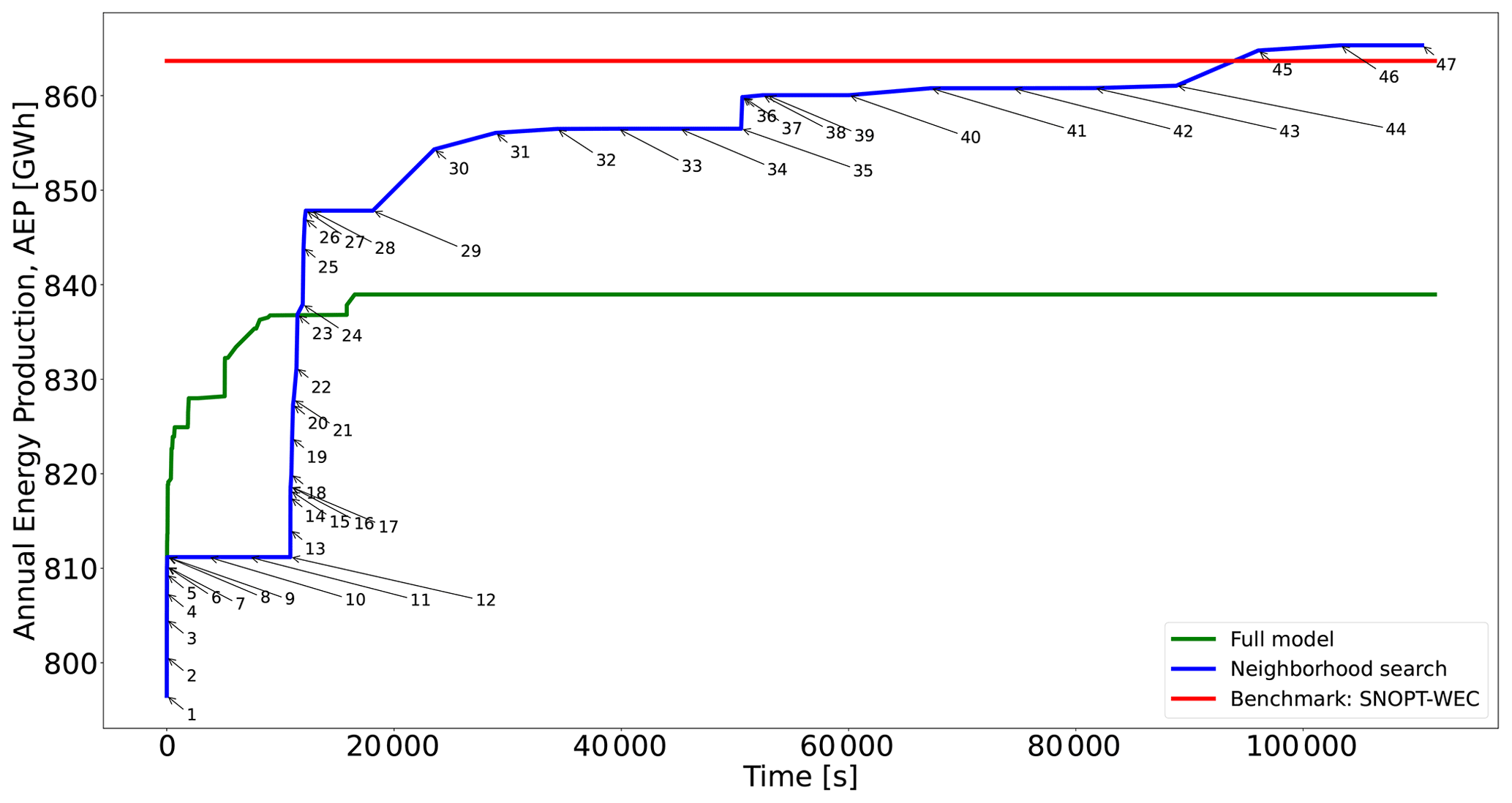
Figure 7 Performance of two different optimization approaches for Case II and comparison with existing best benchmark results. See Table B1 for detailed information about each numbered point in the blue curve.

After a 3 h plateau linked to $\mathrm{8}\le K\le \mathrm{36}$ (four iterations), N is raised to 684, resulting in the largest AEP enhancement, as shown in Fig. 7. The energy production increases by 4.51 % after only 23 min at point 27. This noticeable improvement comes after solving models with rather small neighborhood search sizes of $\mathrm{2}\le K\le \mathrm{4}$ to optimality. The convenience of allowing for large neighborhood search sizes such as K=16 or K=36 is reflected at this moment. From point 30 to 33 (6 h) with K=16 the incumbent is slowly boosted by nearly 1 %. Again, after a 3 h plateau, N becomes equal to 1907, and after around 32 min for $\mathrm{2}\le K\le \mathrm{4}$, the AEP is augmented by 0.41 %. Then, the large neighborhood search starts for K=16 and K=36, and after a total of 16 h, the final solution of 865 GW h (increment of 0.61 %) is achieved (Fig. 8b).

The full model (i.e., without implementing the NSH algorithm) initially provides better solutions within the first 3 h but then lags behind in solution quality compared to the NSH algorithm in the long run (lower by 3.05 %), as shown in Fig. 7.

For this case, the proposed method reaches the best solution, as shown in the fifth column of Table 2. The SNOPT + WEC is again the closest contender. When uniquely compared to GF methods, the proposed method matches the best solution from those algorithms after around 3 h, which is generally a reasonable amount of computing time compared to methods where gradients are not explicitly utilized in the optimization process, especially for metaheuristics such as genetic algorithms or swarm optimization.

Figure 8 Generated wind farm layouts for benchmark Case II with 36 wind turbines.

5.4 Case III: 64 WTs

This case has a round shape with a radius of 3000 m and n_T=64 WTs. The evolution of the proposed methods and the initial and final WT layouts are displayed in Figs. 9 and 10, respectively. Table C1 displays the data linked to each point of Fig. 9. The main inputs are $\mathbf{C}=\left\{\mathrm{625},\mathrm{1017},\mathrm{2741}\right\}$, $\mathbf{T}=\left\{\mathrm{1},\mathrm{1.5},\mathrm{2}\right\}$ h, and $\mathbf{V}=\left\{\mathrm{2},\mathrm{4},\mathrm{8},\mathrm{16},\mathrm{32},\mathrm{64}\right\}$. Note that in comparison the number of elements of V has been increased by one after each study case. This has been done while taking into account the number of WTs. Likewise, the values of N∈C are larger to cover for the wider project areas.

Comparing the blue lines of Figs. 5, 7, and 9, it becomes evident that for the last case the curve shows less sudden increases. The largest change occurs after 27 s, where the initial solution (Fig. 10a) with an AEP of 1395 GW h is improved by 3.18 % for N=625 and K=2 up to point 9, reaching optimality in a few seconds. With $\mathrm{4}\le K\le \mathrm{8}$ the model instantiations are solved to optimality in minutes, obtaining a solution improved by 0.18 %.

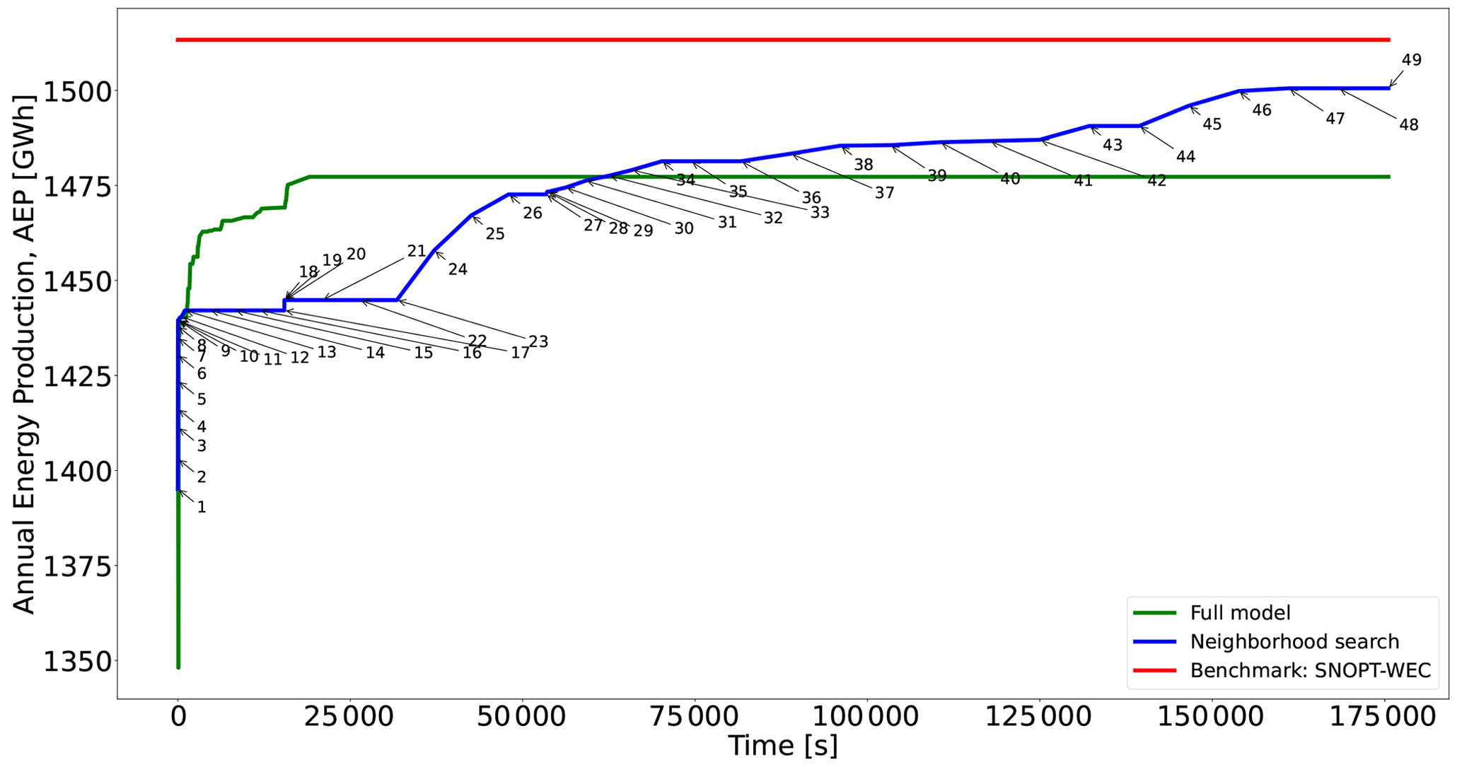
Figure 9 Performance of two different optimization approaches for Case III and comparison with existing best benchmark results. See Table C1 for detailed information about each numbered point in the blue curve.

Figure 10 Generated wind farm layouts for benchmark Case III with 64 wind turbines.

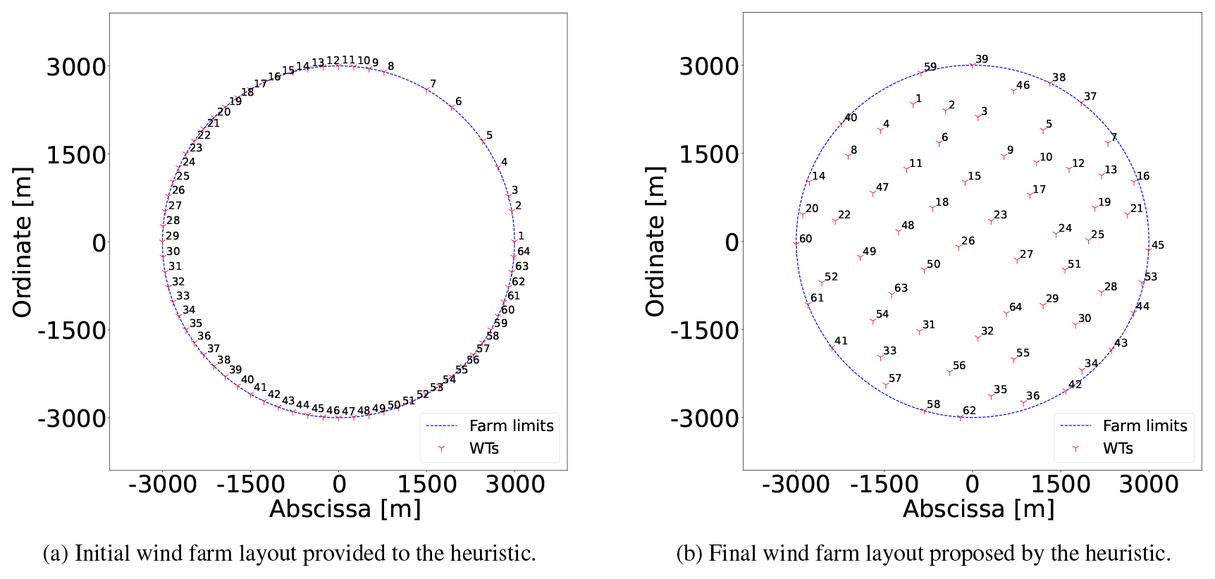
After point 13 in Fig. 9, one notes a plateau without improvement for N=625 and K≥16; i.e., a large neighborhood search does not lead to further enhancements. Due to this, N is enlarged to 1017, where the second largest boost (increase of 2.12 %) comes, with the largest search size (K=64) resulting in the best improvement. This enhancement occurs 13 h after starting the NSH (point 26). From point 28, N=2741 and for $\mathrm{2}\le K\le \mathrm{4}$ the solver reaches optimality, slowly converging to the final solution of 1500 GW h (Fig. 10b).

The seventh column of Table 2 shows that the SNOPT + WEC and the preconditioned SQP provide slightly better layouts than the proposed method. However, the algorithm provides feasible layouts that improve the objective compared to all the gradient-free approaches.

5.5 Case IV: 10–50 WTs

Although in most projects today the total capacity for grid connection is already decided in the early planning phases, in the future one can envisage situations where flexibility in optimizing the number of wind turbines in a project would yield benefits.

Even if the power-curve-free model (Sect. 3.2) exhibits quite good performance in terms of the AEP and computing time for a fixed number of WTs (when the AEP and NPV are basically the same metric), it is not very applicable for when a variable number of wind turbines are considered. Based on computational experiments not included in the paper, the power-curve-free model embedded in the NSH terminates too early in the search process, resulting in a solution worse than the alternative discussed below.

For such an optimization, the power-curve-based mathematical program of Sect. 3.1 may be handy as the number of generators is allowed to vary between a lower and upper bound of n^min and n^max, respectively. For illustrative purposes, a domain defined by a circle with a radius of 1300 m and a variable number of WTs of between 10 and 50 are utilized. These parameters are set relatively arbitrarily but with a sufficient distance so as to reasonably expect that the limits are not reached. The aim is to illustrate the ability of the method in reaching non-trivial solutions, resulting in an optimized design with an intermediate number of wind turbines.

Keeping that in mind for this case, a linear superposition model for the AEP component in the NPV calculation is considered. In this sense, the original WT power curve as depicted in Fig. 1 is used. The NPV is the true objective function when applying the NSH of Algorithm 1. The modified objective function of MILP model of Eq. (18) for this case has the form (Cogency, 2014)

$$\begin{array}{}\text{(25)}& \underset{\mathit{\xi },\mathit{\eta },u}{\text{maximize}}-\sum _{i=\mathrm{1}}^N{c}_{\text{wt}}{\mathit{\xi }}_i+\mathrm{8760}\sum _{y=\mathrm{1}}^Y\sum _{i=\mathrm{1}}^N\sum _{j,k}\sum _{l=\mathrm{1}}^{m+\mathrm{2}}{\displaystyle \frac{c_{\mathrm{e}}{w}_{jk}{\mathit{\eta }}_{ijk}^{l}p\left(u_m^l\right)}{(\mathrm{1}+r{)}^y}},\end{array}$$

where c_wt is the cost per WT (m EUR), c_e is the energy price (m EUR MW h⁻¹), r is the discount rate (%), and Y is the number of years of lifetime of the project. For this case study, values of c_wt=6.7 m EUR (Mishnaevsky and Thomsen, 2020), c_e=0.00015 m EUR MW h⁻¹ (Nord Pool, 2022), r=5 %, and Y=20 are assumed. The general form of the NPV equation as per Cogency (2014) is defined by the sum of the present value of cash flows (discounted cash flow, DCF) of a project under analysis. In Eq. (25), the first sum is a negative cash flow representing the purchase of the WTs at the construction stage of the project, while the next term represents positive cash flows coming from trading the electricity in the market. Because of the additive nature of the NPV metric and since the focus is on evaluating investment vs. revenues, by maximizing Eq. (25), a fully comprehensive NPV metric is equivalently improved.

The model of Eq. (18) with the modified objective function of Eq. (25) embedded in the NSH algorithm 1 with the NPV as the target function is executed in three runs. For the first run the number of turbines is fixed to $n^{min}=n^{max}=\mathrm{10}$, while for the second the number of turbines remains fixed but is increased to $n^{min}=n^{max}=\mathrm{50}$. For the third run the number of wind turbines is allowed to vary between $n^{min}=\mathrm{10}$ and $n^{max}=\mathrm{50}$. The Algorithm 1 input parameters are $\mathbf{C}=\left\{\mathrm{467},\mathrm{590},\mathrm{1014}\right\}$, $\mathbf{T}=\left\{\mathrm{1},\mathrm{1.5},\mathrm{2}\right\}$ h, and $\mathbf{V}=\left\{\mathrm{2},\mathrm{4},\mathrm{6},\mathrm{8},\mathrm{24}\right\}$. The results are plotted in Fig. 11.

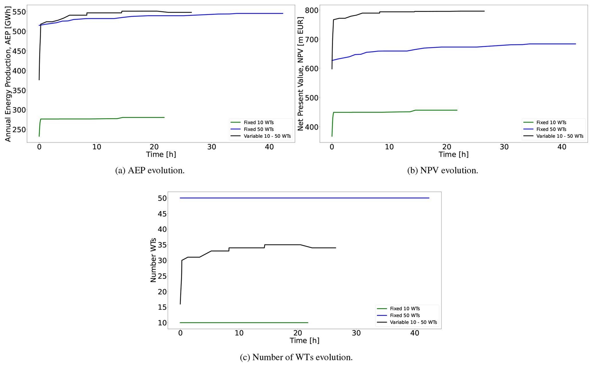
Figure 11 Evolution of the AEP, NPV, and number of WTs for the three simulations. The green lines are results for the optimization program with a fixed number of WTs equal to 10, and the blue lines are equal to 50; the black lines are for the optimization program with a variable number of WTs between 10 and 50.

When the number of turbines is fixed to 10, the NPV evolution (green line in Fig. 11b) is driven by the AEP (green line in Fig. 11a). Both curves are monotonically increasing, reaching a final value of the NPV of =456.40 m EUR. The same behavior is visible for n_T=50, although the final NPV is greater (683.53 m EUR) (see the blue line in Fig. 11b). In the second study, the positive difference in DCF from the revenues surpasses the associated extra investment costs from the additional 40 wind turbines considered. The significant increase in the number of WTs doubles the computing time, due to the large increase in the number of variables; selecting 50 WTs entails significantly more possible combinations of valid points.

An interesting question is whether there is a larger NPV in between the bounds of the WT number. For the optimization program with a variable number of WTs, the evolution of the WT number in Fig. 11c and the AEP in Fig. 11a (see black lines in these figures) exhibits a perfect correspondence. The more WTs, the larger AEP, in spite of the increased wake losses. The curves increase with time, up to a point where the model estimates that a further increase in WTs would not lead to a better NPV. The final number of WTs is 34. The NPV evolution in Fig. 11b (black line) naturally only improves with time, resulting in a final value of 795.86 m EUR. Note that the NPV in this case is greater than when a larger number of WTs (i.e., 50) was considered and of course when only 10 were considered. Interestingly, the optimization program with a fixed number of 50 WTs finds a final solution with an AEP very close to that from the variable number program, which is the solution of the former, 0.50 % lower than the latter but requiring more WTs and hence more investment (47 % more). The final NPV value of the variable number model is 16.43 % greater than the one with a fixed number of 50 WTs. These figures could be expected to be similar even in situations where lower AEPs are obtained if that compensates by augmenting overall financial metrics such as the NPV.

This result shows the benefit of having optimization models that support a variable number of WTs and accounting for metrics beyond the AEP. The advantages may become even more pronounced for more complex situations, such as, for instance, if the WT investment costs are dependent on the exact installation area or different WT sizes are considered.

6 Discussions

The two models proposed in this paper have many of the characteristics of mixed-integer linear programming models. They require significant computational time and memory and exhibit rather low tractability and scalability for global optimization algorithms.

The power-curve-based model, although requiring more computational resources, manages to provide reasonably good solutions for a small-sized problem, being only 1.18 % lower than its power-curve-free counterpart for the case with 16 WTs and 4.41 % for the case with 36 WTs. This diminishing efficiency is to be expected, given the large number of variables and constraints. The power-curve-free model on the other hand, along with the heuristic, is much faster due to its more compact formulation. This translates into the ability to be highly competitive compared to a large set of benchmark algorithms. In situations where there is an interest in optimizing metrics beyond the AEP, such as the NPV, the power-curve-based model becomes very useful given its intrinsic capacity to support this kind of objective functions.

It should be mentioned that there are limitations for the wake models used compared to recent ones (Thomas et al., 2022). For example, the wake model used in this paper does not consider the changes in the turbulence intensity or thrust coefficient variations from wind speed variations inside the wind farm. It is uncertain if using wake models like the ones in Thomas et al. (2022) would still allow for an integer linear programming formulation or approximation of the WFLO problem. The impact on the final solution quality these detailed modeling aspects imply is also uncertain. These questions are left for future work.

Notwithstanding the listed shortcomings, it is enthralling that these models, in combination with the neighborhood search heuristic, are able to match and in some cases improve upon the results obtained when considering the turbine positions as continuous variables (see Table 2). This opens the door to experimental case studies with functionalities easily adaptable to discrete parameterization techniques, which can be very challenging for approaches of continuous-variable modeling.

7 Conclusions

This paper contributes both methodologically and empirically to address the WFLO problem. A neighborhood-search-heuristic-embedding integer programming formulation is proposed. For both presented formulations presented in the paper, the stepwise power curve and power-curve-free model, the heuristic notably improves a single execution of full models when calling a state-of-the-art branch-and-cut solver in terms of solution quality. An improvement of up to 3.42 % in the AEP is achieved by applying the neighborhood search strategy for cases where the WT number is fixed compared to solving the full model.

Another important takeaway is the satisfactory performance of the power-curve-free model, which uses an approximation of the total wind speed deficit, when (implicitly) optimizing for the AEP. This is due to the good correlation between the two measures and the correction capability of the heuristic. For the classic WFLO problem definition, the proposed model is able to considerably improve (from 1 % to around 10 %) the AEP compared to benchmark results by multiple gradient-based and gradient-free algorithms. Even when directly compared to methods implementing a continuous-variable technique, the proposed heuristic provides similar or even better results. These are very promising results that would enable getting high-quality solutions for problem instances where continuous-variable modeling approaches may not be able to run or provide with good incumbents.

Finally, the model with an explicit representation of the power curve embedded within the neighborhood search heuristic is able to propose non-trivial solutions when implementing objective functions beyond the AEP, such as the NPV. For these cases, the trade-off between energy revenues and investment costs is studied. For example, the model suggests that installing a lower number of wind turbines than allowed would result in a better NPV value, with a comparable AEP.

Appendix A: Case I

Table A1 Information about the values of N, K, and T and the termination criterion of the solver after each point in Fig. 5.

Appendix B: Case II

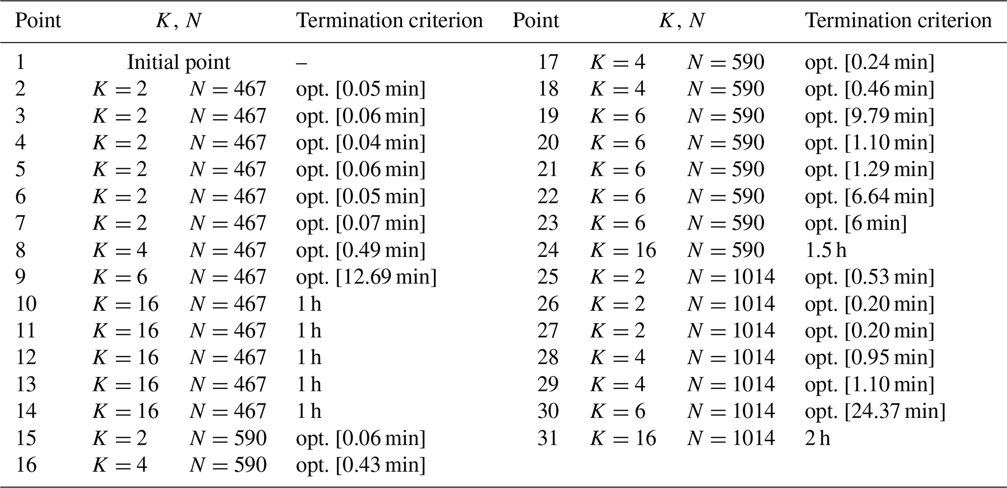
Table B1 Information about the values of N, K, and T and the termination criterion of the solver after each point in Fig. 7.

Appendix C: Case III

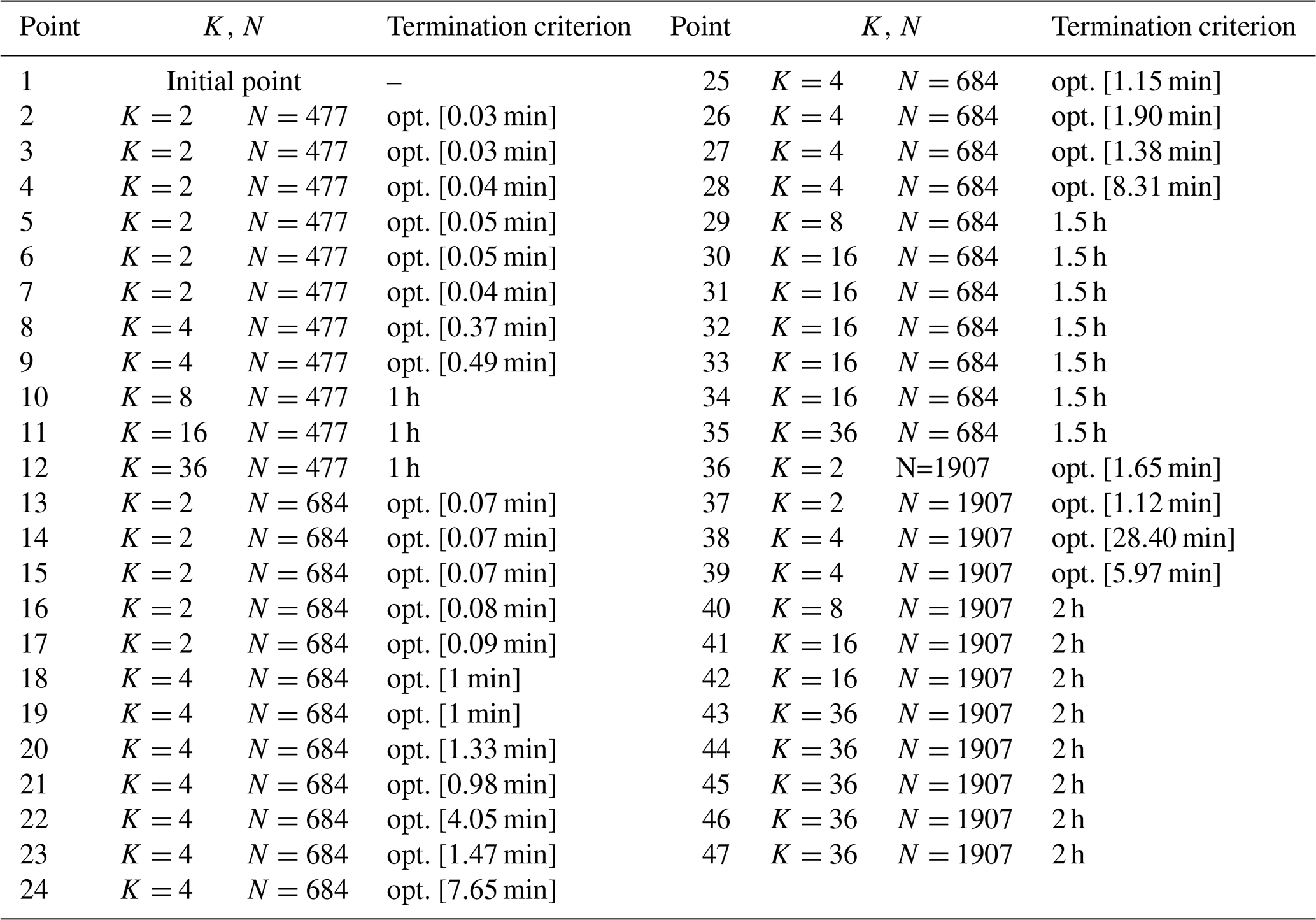
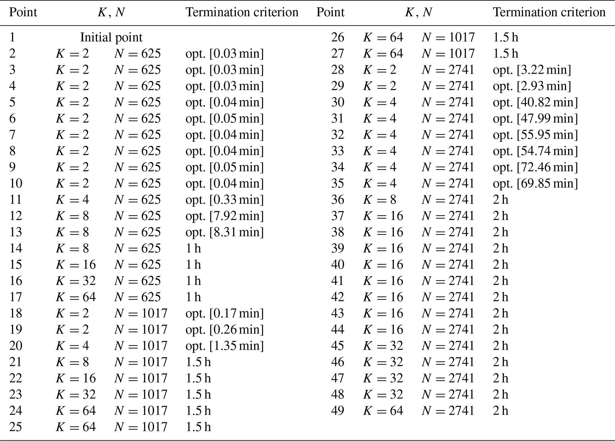
Table C1 Information about the values of N, K, and T and the termination criterion of the solver after each point in Fig. 9.