A decision-tree-based measure–correlate–predict approach for peak wind gust estimation from a global reanalysis dataset

Peak wind gust (W_p) is a crucial meteorological variable for wind farm planning and operations. However, for many wind farm sites, there is a dearth of on-site measurements of W_p. In this paper, we propose a machine-learning approach (called INTRIGUE, decIsioN-TRee-based wInd GUst Estimation) that utilizes numerous inputs from a public-domain reanalysis dataset and, in turn, generates multi-year, site-specific W_p series. Through a systematic feature importance study, we also identify the most relevant meteorological variables for W_p estimation. The INTRIGUE approach outperforms the baseline predictions for all wind gust conditions. However, the performance of this proposed approach and the baselines for extreme conditions (i.e., W_p>20 m s⁻¹) is less satisfactory.

1 Introduction

Wind gust or gusty wind is a common household term. However, there has yet to be a consensus on its exact scientific definition. For example, according to the Glossary of Meteorology (AMS, 2023), a wind gust can be defined as follows:

A sudden, brief increase in the speed of the wind. It is of a more transient character than a squall and is followed by a lull or slackening in the wind speed. … According to U.S. weather observing practice, gusts are reported when the peak wind speed reaches at least 16 knots and the variation in wind speed between the peaks and lulls is at least 9 knots. The duration of a gust is usually less than 20 s.

A somewhat different definition has been suggested by the US National Oceanic and Atmospheric Administration (NOAA, 2023):

A rapid fluctuation in wind speed with variation of 10 knots or more between peaks and lulls.

As opposed to these quantitative definitions, the World Meteorological Organization (WMO, 2021, p. 227) describes wind gusts in a very generic way:

The extent to which wind is characterized by rapid fluctuations is referred to as gustiness, and single fluctuations are called gusts.

Despite these vast differences in the definition of wind gusts, most sources seem to agree on the meaning of “peak” wind gusts (W_p):

The maximum observed wind speed over a specific time interval. (WMO, 2021, p. 227)

On the basis of this definition, it is appropriate to assert that “peak gust need not be a true gust of wind” (AMS, 2023). For quiescent atmospheric settings, within certain time periods, peak wind gusts may very well be close to near-calm conditions. While in the presence of certain meteorological phenomena (e.g., downbursts, tornadoes), they may attain severe, hazardous intensities. The focus of the current study is on the estimation of a wide range of peak wind gusts using a decision-tree-based (DT) machine-learning (ML) approach.

Measurements of W_p require high-frequency observations. Typically, cup, propeller, and sonic anemometers record wind speeds with sampling rates of O(1–10) Hz. First, block averaging is performed on these measured time series with a window length of τ (in seconds). Subsequently, for a specific time period T, the maximum (or peak) of the τ-averaged values (in seconds) is estimated, which is known as the τ (in seconds) peak wind gust (Panofsky and Dutton, 1984; Holmes, 2001; Solari, 2019). The magnitude of W_p strongly depends on the selected values of τ and T (Brook and Spillane, 1968; Beljaars, 1987). Most commonly, τ is chosen to be equal to a few seconds. Depending on the application, the value of T can be as small as a few minutes to as large as several hours. For example, the Automated Surface Observing System (ASOS) employed by the US National Weather Service measures 5 s peak wind gusts and considers a time period of 1 min. In contrast, in the wind energy literature (Rohatgi and Nelson, 1994), the combination of τ=3 s and T=10 min is more prevalent. From a wind engineering perspective, a historical account of 3 s for W_p has recently been documented by Lombardo (2021).

If the mean and peak gust wind speeds during T are denoted by W and W_p, respectively, then one can write (Holmes, 2001)

$$\begin{array}{}\text{(1)}& W_{\mathrm{p}}=W+c{\mathit{\sigma }}_{\mathrm{W}}.\end{array}$$

Here σ_W is the standard deviation of wind speed. If the high-frequency wind speed data follow a Gaussian distribution during T, then c can be approximately equal to 3.5 (≈ 99.98th percentile). Equation (1) can be re-written as

$$\begin{array}{}\text{(2a)}& W_{\mathrm{p}}=W\left(\mathrm{1}+c{\displaystyle \frac{{\mathit{\sigma }}_{\mathrm{W}}}{W}}\right)\end{array}$$

or

$$\begin{array}{}\text{(2b)}& G={\displaystyle \frac{W_{\mathrm{p}}}{W}}=\left(\mathrm{1}+c{\displaystyle \frac{{\mathit{\sigma }}_{\mathrm{W}}}{W}}\right).\end{array}$$

The ratio G is the so-called gust factor, whereas the ratio $\frac{{\mathit{\sigma }}_{\mathrm{W}}}{W}$ is known as the turbulence intensity (TI).

In the wind energy literature, several studies (Sumner and Masson, 2006; Wharton and Lundquist, 2012; Hedevang, 2014; Siddiqui et al., 2015; St. Martin et al., 2016; Lee et al., 2020) have reported on the (negative) impacts of high TI on power production. Given the linear relationship between G and TI, it is expected that high-value gust factors may also be responsible for sub-optimal wind power production. Highly fluctuating power production due to wind gusts may also cause problems for electrical grid balancing (Milan et al., 2013). In addition to power production, high TI (or G) also induces significant fatigue loading on wind turbines (Kelley et al., 2000; Hansen and Larsen, 2005; Dimitrov et al., 2017; Ebrahimi and Sekandari, 2018; Ren et al., 2018; Asadi and Pourhossein, 2021).

Contemporary wind turbine design standards (e.g., IEC, 2019) include provisions for extreme weather conditions. Some of them are related to extreme wind gusts (e.g., extreme coherent gust with direction change, extreme operating gust). Severe meteorological phenomena, such as thunderstorm downbursts, tornadoes, and hurricanes, can generate extreme wind gusts. We document a few historical events of relevance. One of the highest-ever recorded gusts was recorded at Andrews Air Force Base on 1 August 1983 (Fujita, 1985). Due to the passage of a microburst, near-surface gust speed reached approximately 130 knots (≈67 m s⁻¹). The airplane of US President Ronald Reagan landed just 6 min before this extreme gust event. This extreme event provided the necessary stimulus to mobilize extensive research on microburst phenomena in the 1980s. Petersen et al. (1998) documented an even stronger gust event in a review paper on wind power meteorology. They analyzed wind data during a storm event on the Faroe Islands. There, prior to collapsing, one of the instrumented met towers registered a gust value of 76.7 m s⁻¹. It is entirely possible that these types of severe gust events might hamper the structural integrity of modern-day wind turbines. About 20 years ago, one such event took place on Miyako-jima in Japan. The recorded maximum gust speed was 74.1 m s⁻¹. Out of six turbines, three turbines entirely collapsed, and the other ones sustained significant damage (Ishihara et al., 2005). A more recent event was documented by Hawbecker et al. (2017). A thunderstorm producing multiple downbursts and tornadoes passed through the Buffalo Ridge Wind Farm, Minnesota (USA), in 2011. The resulting wind gusts caused damage to turbine blades and also caused buckling of a turbine tower.

Based on the aforementioned published studies and other anecdotal evidence, we can conclude that both nominal and extreme wind gusts are critical for wind energy. Therefore, during the wind farm planning and operation stages, the (detrimental) effects of wind gusts should be adequately accounted for. However, it is widely known in the literature that wind gusts are spatially and temporally highly intermittent. Thus, the long-term statistical characterization of such events utilizing on-site wind sensors is rather challenging and expensive. As an alternative, mesoscale meteorological models (MMMs) can be used to predict and forecast peak wind gusts (Goyette et al., 2003; Ágústsson and Ólafsson, 2009; Stucki et al., 2016; Kurbatova et al., 2018). Typically, different physical parameterizations are used for convective and non-convective gusts (refer to Sheridan, 2011, and the references therein). Although these physical parameterizations have improved over the years, considerable improvements can still be made. It is also important to note that MMMs are computationally expensive, especially when sub-kilometer grids and gray-zone physical parameterizations (Boutle et al., 2014; Shin and Hong, 2015) are used. In this paper, we propose a data-based alternative approach that leverages a decision-tree-based technique for peak wind gust estimation from a global reanalysis dataset. We name the proposed approach INTRIGUE (decIsioN-TRee-based wInd GUst Estimation). It requires limited (say 1 year) on-site W_p data for training and can generate a multi-year W_p time series for that specific site. It also performs reasonably well for generating W_p data for neighboring sites. Most importantly, separate parameterizations for convective and non-convective events are not required.

The structure of this paper is as follows. Since the proposed INTRIGUE approach uses various meteorological input features (e.g., friction velocity; CAPE, convective available potential energy), we briefly summarize a few relevant physical parameterizations in Sect. 2. In Sect. 3, we include a concise literature review on various applications of ML in wind-gust-related research. Descriptions of the study area and relevant datasets are provided in Sects. 4 and 5, respectively. Various technical details pertaining to the INTRIGUE approach (e.g., data splitting, hyperparameter turning) are elaborated in Sect. 6. In Sect. 7, we report all the results including a discussion on feature importance. The limitations of the INTRIGUE approach for extreme wind gusts are mentioned in Sect. 8. Concluding remarks and future perspectives are provided in Sect. 9.

2 Physical parameterizations of peak wind gusts

In a technical report, Sheridan (2011) provided a comprehensive review of various physical parameterizations for peak wind gusts. A few years later, Kurbatova et al. (2018) investigated the capabilities of seven of these parameterizations in forecasting gusts in Russia. Here, we briefly mention a few well-known (and simple) parameterizations. Unless stated explicitly, we assume W and W_p are defined at the height of 10 m a.g.l. (above ground level).

It is well known in the literature that the gust factor (G) depends on τ, T, measurement height, wind direction, surface roughness, and other factors (Wieringa, 1973; Ashcroft, 1994; Weggel, 1999; Choi and Hidayat, 2002; Harris and Kahl, 2017). However, for simplicity, in a constant gust factor parameterization, G is assumed to be equal to a constant c_GF:

$$\begin{array}{}\text{(3)}& G={\displaystyle \frac{W_{\mathrm{p}}}{W}}=c_{\mathrm{GF}}.\end{array}$$

A few climatological studies have found that even though G varies significantly with respect to underlying topography, the spatially averaged value of G is not site-specific. For example, Harris and Kahl (2017) analyzed multi-year, high-resolution ASOS data from Milwaukee, Wisconsin (USA), and reported an average value of c_GF=1.74. While analyzing Santa Ana winds in southern California (USA), Fovell and Cao (2017) found c_GF=1.6–1.7 to be representative of two locations. Based on multi-year observational data from more than 30 stations in Switzerland, Stucki et al. (2016) estimated c_GF to be equal to 1.67.

The following surface layer similarity-based formulation is also often used for non-convective conditions (Sheridan, 2011; Stucki et al., 2016):

$$\begin{array}{}\text{(4)}& W_{\mathrm{p}}=W+c_{u_{*}}{u}_{*}.\end{array}$$

Here u_* is the so-called surface friction velocity. The coefficient $c_{u_{*}}$ is on the order of 7.5. Sometimes, in Eq. (4), a non-linear function of the stability parameter is used in conjunction with the $c_{u_{*}}{u}_{*}$ term (e.g., ECMWF, 2020).

Certain non-convective formulations make use of boundary layer height (H, in m) and/or wind speed at the boundary layer height (W_H) in a semi-empirical manner. Stucki et al. (2016) reported one such formulation:

$$\begin{array}{}\text{(5)}& W_{\mathrm{p}}=W+\left(W_{\mathrm{H}}-W\right)\left(\mathrm{1}-{\displaystyle \frac{H}{\mathrm{2000}}}\right).\end{array}$$

Brasseur (2001) proposed an interesting physically based approach for gust estimation. It assumes that the gusts at the surface originate from the upper part of the boundary layer. Since the formulation is somewhat involved, we do not include it here. However, we do point out that it includes vertically averaged turbulent kinetic energy ($\stackrel{\mathrm{‾}}{e}$) as a key variable.

In the proposed INTRIGUE approach, we use W, u_*, H, and several other relevant meteorological variables (e.g., surface sensible heat flux, CAPE). If a relevant variable is not available as an input feature, we use our domain knowledge to include a surrogate variable. For example, $\stackrel{\mathrm{‾}}{e}$ is not available in the global reanalysis dataset that we used. Hence, as a substitute, we make use of the average energy dissipation rate ($\stackrel{\mathrm{‾}}{\mathit{\epsilon }}$) in the boundary layer. The relationship between $\stackrel{\mathrm{‾}}{e}$ and ε has been studied in the literature (e.g., Basu et al., 2021). In Sect. 7 of this paper, we perform a systematic feature importance study and show that most of the variables included in well-known physical parameterizations (e.g., Eqs. 3–5) also turn out to be very important from a purely data-based ML standpoint.

3 Applications of ML in wind gust research

To the best of our knowledge, only a handful of studies (Mercer et al., 2008; Sallis et al., 2011; Chaudhuri and Middey, 2011; Carcangiu et al., 2014; Patlakas et al., 2017; Wang et al., 2020; Spassiani and Mason, 2021; Schulz and Lerch, 2022; Wang et al., 2022) have incorporated machine-learning approaches for wind-gust-related research. Several of these studies focused on extreme wind gusts. For example, Mercer et al. (2008) studied downslope windstorms in Colorado (USA). They compared the performance of stepwise linear regression, support vector regression, and multilayer perceptrons in short-term forecasting of extreme wind gusts. They utilized various meteorological variables (e.g., 700 hPa wind speed, mountaintop relative humidity) and parameters derived from radiosondes (e.g., integrated Scorer parameter, Sangster parameter) as input features. In another study, Chaudhuri and Middey (2011) used ML approaches for predicting peak wind gusts associated with pre-monsoon thunderstorms near Kolkata (India). Their newly developed adaptive neuro-fuzzy inference system outperformed multiple linear regression, a radial basis function network, and multilayer perceptrons.

Various ML approaches (e.g., Kalman filtering, Gaussian process regression) were also utilized for short-term forecasting of wind gusts. Some of these studies post-processed numerical weather prediction data (e.g., Patlakas et al., 2017; Schulz and Lerch, 2022; Wang et al., 2022). In contrast, Wang et al. (2020) only used observed time-series data from Jiangsu Province (China) for forecasting. They used an ensemble-learning method comprising of random forest, long short-term memory, and Gaussian process regression. In order to mitigate wind turbine loads, Carcangiu et al. (2014) proposed a multilayer perceptron for gust detection followed by an innovative turbine control strategy.

Numerous studies (e.g., Enloe et al., 2004; Azorin-Molina et al., 2016; Brázdil et al., 2017; Lombardo and Zickar, 2019) have reported climatologies and in-depth statistical analysis of wind gusts in various countries. However, they do not leverage any ML approaches. An exception is the study by Spassiani and Mason (2021). They used self-organizing maps (Kohonen, 1990, 2013) to perform automated classification of wind gusts in Australia in order to identify their dynamical origins.

It is important to stress that the scope of the present study is different from these past ML-based investigations. We are interested in generating long-term, site-specific peak wind gust (W_p) series based on a global reanalysis dataset. Our proposed INTRIGUE approach, described in Sect. 7, can be described as an advanced measure–correlate–predict (MCP) approach for peak wind gusts. MCP is well established in wind resource estimation (e.g., Rogers et al., 2005; Carta et al., 2013). However, its usage in peak wind gust estimation is not known to us.

4 Study area

This study focuses on the Texas Panhandle region, one of the largest semi-arid regions in the world. This region's major distinguishing topographical feature is the Caprock Escarpment (see the top-left panel of Fig. 1), a precipitous cliff with an average height of ∼90 m. Otherwise, this region is very flat, homogeneous, and sparsely vegetated. Owing to the frequent occurrence of strong nocturnal low-level jets, the wind resource of this region is very good (wind class 3–5). This fact has led to the construction of numerous wind farms in this region, some of which (e.g., Roscoe, Horse Hollow, Buffalo Gap, Sweetwater) are among the largest operating wind farms in the US.

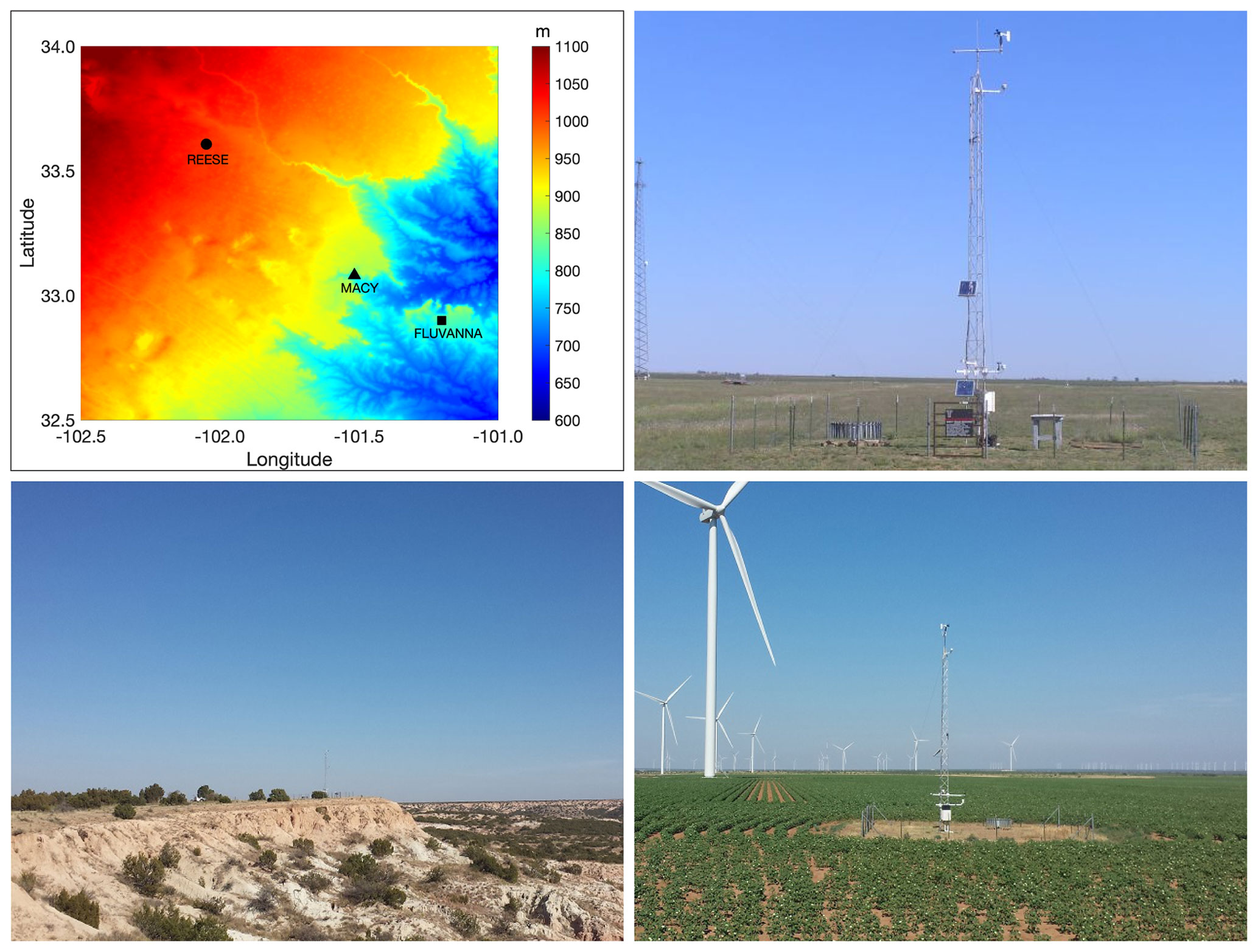
Figure 1 Top-left panel: digital elevation map of the study area. The symbols denote the locations of three West Texas Mesonet stations. Photographs of the REESE (Reese Technology Center, Lubbock County), MACY (Garza County), and FLUVANNA (Borden County) stations are shown in the top-right, bottom-left, and bottom-right panels, respectively. These photographs were downloaded from https://www.mesonet.ttu.edu/ (last access: 14 October 2023).

The West Texas Mesonet (henceforth WTM) is a high-density network of automated surface meteorological stations which spans the Texas Panhandle region and extends to some parts of New Mexico and Colorado. This network (https://www.mesonet.ttu.edu/, last access: 14 October 2023) was established in 1999 by the Atmospheric Science Group at Texas Tech University (Schroeder et al., 2005).

For the purpose of this study, we have selected three WTM stations (called REESE, MACY, and FLUVANNA) which are located in areas of varying topographical complexities. Their locations are demarcated by various symbols in the digital elevation map of Fig. 1. The station at the Reese Technology Center (REESE) is located at 33^∘36^′26^′′ N, 102^∘02^′55^′′ W, at an elevation of 1021 m, about 19 km west of the city of Lubbock, Texas. The topography is very flat surrounding this station (see the photograph in the top-right panel of Fig. 1). The MACY station is located at the edge of the Caprock Escarpment (bottom-left panel of Fig. 1). Given the complex topographical surroundings, more gusty wind conditions are prevalent at this site. The latitude, longitude, and elevation of this station are 33^∘4^′53^′′ N, 101^∘30^′58^′′ W, and 874 m, respectively. The FLUVANNA station is situated on a relatively flat area off the Caprock Escarpment (refer to the bottom-right panel of Fig. 1). However, a few kilometers away from the station, the ruggedness of the topography increases substantially. This station is located at 32^∘53^′57^′′ N, 101^∘12^′7^′′ W, at an elevation of 826 m, about 105 km southeast of Lubbock, Texas.

5 Description of observed and reanalysis datasets

Each station in the WTM network measures a multitude of meteorological variables. However, in this study, we only utilize the 3 s peak wind gust (W_p) data from the REESE, MACY, and FLUVANNA stations. The associated anemometers (R. M. Young propeller type) are located at 10 m a.g.l. Technical details about the measuring instruments, data quality control, sensor calibration, and other aspects can be found in Schroeder et al. (2005).

In conjunction with these observed W_p data, we make use of several meteorological variables (including simulated wind gusts) from a global reanalysis dataset known as ERA5 (Hersbach et al., 2020). ERA5 is the fifth-generation reanalysis product of the European Centre for Medium-Range Weather Forecasts. Soon after its introduction, the ERA5 dataset became the preferred reanalysis dataset in the wind power meteorology community. Olauson (2018), Ramon et al. (2019), and Gualtieri (2022), among others, discuss its superior accuracy, lower uncertainty, and higher reliability compared to other global reanalysis datasets.

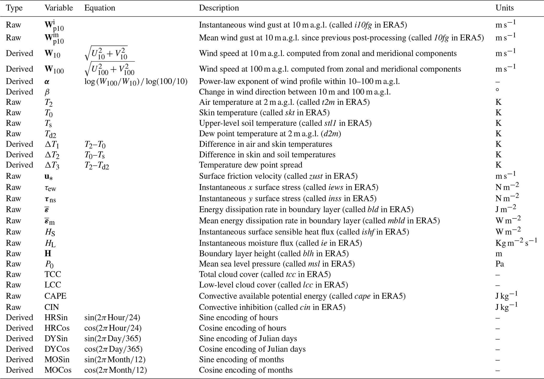
The horizontal resolution of the ERA5 reanalysis dataset is approximately 32 km. For each of the three WTM stations (i.e., REESE, MACY, and FLUVANNA), we have extracted ERA5 data from the corresponding nearest grid points. The distances between the REESE, MACY, FLUVANNA stations and their corresponding ERA5 grid points are 14, 9, and 12 km, respectively. In Table 1, we list some of the extracted ERA5 variables as well as a few derived ones. In total, 265 input features are used in the INTRIGUE approach.

Table 1 A partial list of ERA5 and derived variables utilized as input features for the INTRIGUE approach. The most important variables, identified via permutation feature importance analysis, are printed in bold.

In the ERA5 dataset, snapshots of most of the meteorological variables are output every hour, whereas, in the case of the WTM, the variables are temporally averaged with a sampling rate of 5 min. Direct comparison of point measurements against atmospheric-model-generated gridded data is an ill-posed problem. We do not attempt to resolve this issue in this paper. However, to avoid the sampling-rate mismatch between the WTM and the ERA5 datasets, we pre-process the WTM data with a moving-maxima filter with a non-overlapping window of 1 h. For example, we compute the maximum of contiguous 12 W_p samples measured during 13:30–14:30 CST to estimate the corresponding “hourly” value of W_p at 14:00 CST.

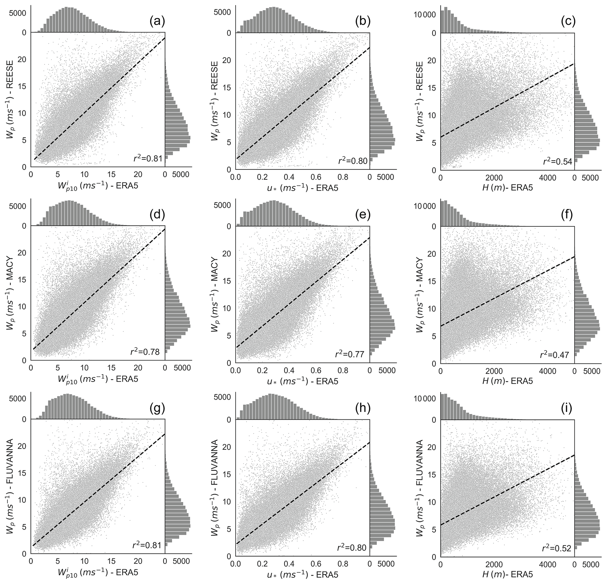
Figure 2 Bivariate histograms of several meteorological variables. On the x axis, the predictor variables from the ERA5 dataset are plotted. The predictor variables are $W_{\mathrm{p}\mathrm{10}}^{\mathrm{i}}$ (a, d, g), u_* (b, e, h), and H (c, f, i). The predictand variable W_p is plotted on the y axis. The top, middle, and bottom panels correspond to the REESE, MACY, and FLUVANNA stations, respectively. To enhance the clarity of these plots, we do not show the data points where W_p>25 m s⁻¹. In the bottom-right corner of each plot, we report the square of the Pearson's correlation coefficient (r). The dashed black lines in these plots represent the linear regression fits.

In Fig. 2, we plot several bivariate histograms. On the x axes, we have the predictor variables – i.e., the meteorological variables from the ERA5 dataset. On the y axes, the peak wind gusts (i.e., W_p) from the WTM stations are shown as predictands. It is evident that both instantaneous wind gusts ($W_{\mathrm{p}\mathrm{10}}^{\mathrm{i}}$) and friction velocity (u_*) from ERA5 are strongly correlated with the measured W_p data (r² is on the order of 0.8). In contrast, the correlations between boundary layer heights (H) from ERA5 and W_p values are much weaker (r²≈0.5). The proposed INTRIGUE approach, described in Sect. 7, exploits not only the strong correlations but also the weaker ones in a systematic manner to provide a more accurate prediction of W_p.

6 Proposed INTRIGUE approach

In the following sub-sections, we describe various technical details associated with the proposed INTRIGUE approach.

6.1 Strategy for the splitting of available data

In this study, we have 11 years (2003 to 2013) of WTM and ERA5 datasets at our disposal. Instead of training various ML models with lots of data, for practical reasons, we have opted for a not-so-abundant training-data scenario. In typical wind resource assessment projects, one has access to merely 1 or 2 years of on-site data. The wind data analysts are then tasked with building MCP models with such a limited amount of data. To mimic this situation, we train ML models with only 1 year of training data and, subsequently, make predictions for 10 years. We repeat this process in a round-robin manner by changing the training and testing years. For example, in the schematic shown in Fig. 3, we use data from the year 2003 for training and make predictions for the years 2004–2013.

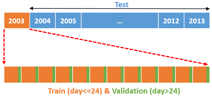
Figure 3 Our strategy of splitting the entire dataset into training, validation, and testing sets.

In ML training, it is customary to hold out a portion of the training data, called a validation set, for hyperparameter tuning. Often an 80 %–20 % randomly shuffled split is made between training and validation sets. However, meteorological data are temporally correlated. Thus, random shuffling causes information leakage into the validation set. To minimize this undesirable leakage problem, we use the first 24 d of each month (i.e., ∼80 %) for training and the rest for validation as depicted in Fig. 3.

6.2 ML models

In this study, we have used four different decision-tree-based ML models. Two of them, random forest (Breiman, 2001) and extremely randomized trees (Geurts et al., 2006), use the so-called bagging approach. The other two approaches, XGBoost (Chen and Guestrin, 2016; Wade, 2020) and LightGBM (Machado et al., 2019), are built on the gradient-boosting technique (Freund and Schapire, 1999; Friedman, 2002). Henceforth, the XGBoost and LightGBM models are referred to as XGB and LGBM, respectively. For a comprehensive treatise on decision trees, bagging, and boosting, the following references are suggested: Rokach and Maimon (2008), Hastie et al. (2009), Géron (2022), and Murphy (2022). We also encourage the readers to peruse the concise tutorial on decision trees by Spiliotis (2022).

It is important to point out that we are interested in comparing the relative performance of various ML approaches for wind gust prediction and identifying if there is a clear winner. It is entirely possible that by combining some of these techniques (e.g., via a stacking regressor), one can get enhanced performance. However, we do not investigate this strategy in this paper.

6.3 Hyperparameter tuning

Each DT-based model contains several hyperparameters (e.g., number of trees, number of tree levels). We include the most relevant ones in Table 2. Technical descriptions of these hyperparameters are beyond the scope of this paper. The readers are encouraged to peruse the original publications and associated code repositories for more information.

Table 2 Hyperparameter search spaces of the bagging and boosting ML models. For each WTM station, different optimized models are constructed. In the last three columns, the best configurations of the models are reported when data from the year 2003 are used for training.

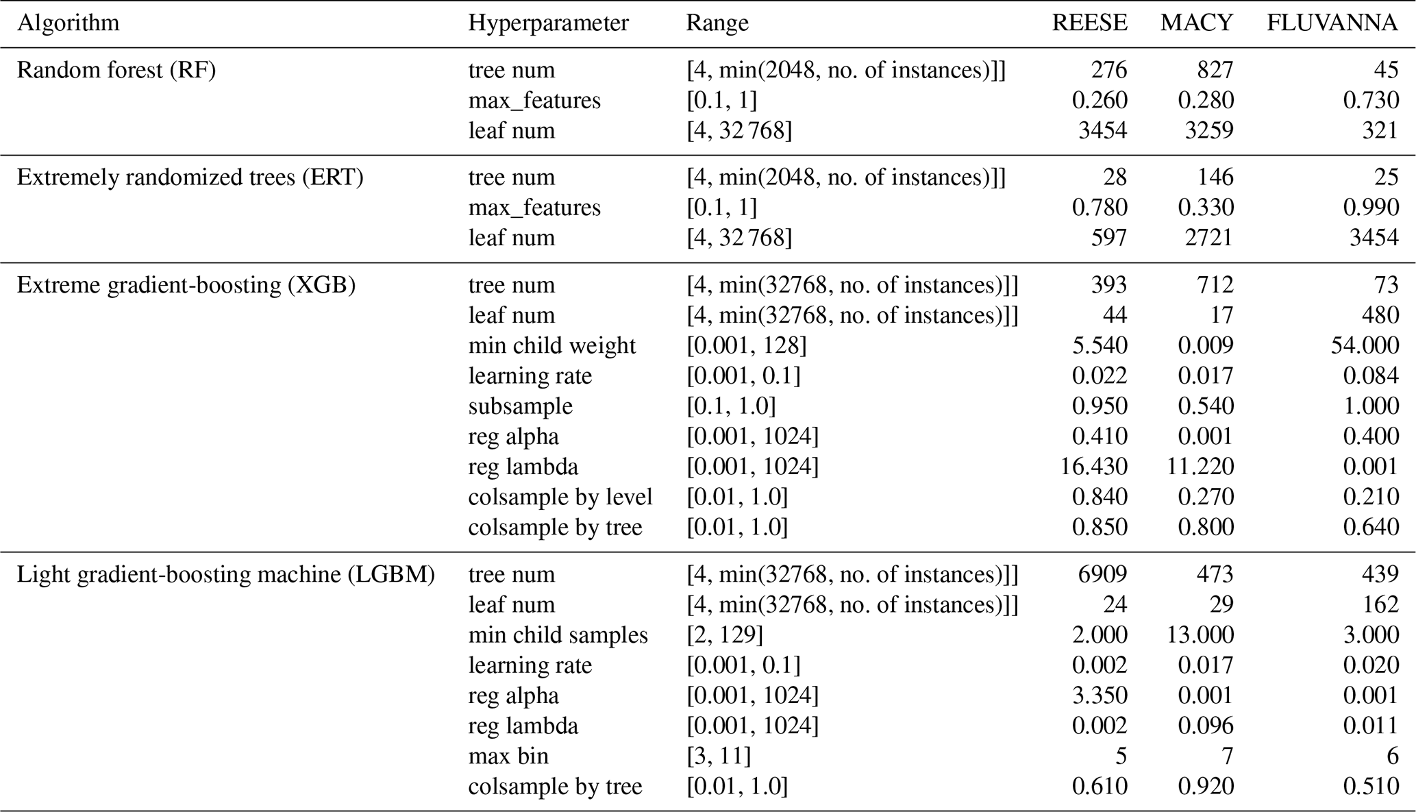
In order to achieve high-level predictive performance, all the hyperparameters should be highly optimized. Quite often, random search or grid search approaches are used (Géron, 2022). These strategies are very time-consuming and may require sophisticated hardware support. As an alternative, in this study, we have used FLAML (A Fast Library for Automated Machine Learning & Tuning), developed by Microsoft (https://microsoft.github.io/FLAML/, last access: 14 October 2023). Instead of performing the grid search, the FLAML library takes the available computing time as a parameter and tries to find the optimal hyperparameters within the allotted time.

FLAML optimizes hyperparameters using effective search strategies. During the search process, the learner decides on the hyperparameter, sample size, and resampling strategy while taking advantage of the combined effects on both cost and error. The design of FLAML is presented in Fig. 3 of Wang et al. (2021). It consists of two layers, an ML layer, and an AutoML (automated machine learning) layer. In the present study, since each ML model (i.e., RF, XGB) is optimized individually; the ML layer contains only the relevant model. The AutoML contains a learner proposer, a hyperparameter and sample size proposer, a resampling strategy proposer, and a controller. While the proposers are used to decide the variables, the controller is used to initiate the experiment using the learner selected in the ML layer. These steps are repeated during the allotted time. The algorithm uses the random direct search method to decide hyperparameters (Wu et al., 2021).

In this study, we focus on three different WTM stations (REESE, MACY, and FLUVANNA). For each station, we have 11 distinct training sets (one for each year). For each training set, we have four DT-based candidate models. In summary, we have a total of $\mathrm{3}\times \mathrm{11}\times \mathrm{4}=\mathrm{132}$ cases of distinct hyperparameter optimizations. To limit the overall computing time, each case is optimized for 1 h on a Windows workstation equipped with an Intel Core i7 3.5 GHz CPU and NVIDIA GeForce GTX 1070 (8 GB) GPU. The total computing time was 132 h. As an example, we provide the best configuration values for the year 2003 in Table 2. In addition, we also provide the search range of each hyperparameter in this table.

6.4 Performance evaluation metrics

For model evaluations, we have used bias, the mean absolute error (MAE), the mean squared error (MSE), and the coefficient of determination (R²) as performance metrics. They are defined as follows:

$$\begin{array}{}\text{(6a)}& {\displaystyle }& {\displaystyle }\mathrm{bias}={\displaystyle \frac{\mathrm{1}}{N}}\sum _{i=\mathrm{1}}^N\left({\widehat{y}}_i-y_i\right),\text{(6b)}& {\displaystyle }& {\displaystyle }\mathrm{MAE}={\displaystyle \frac{\mathrm{1}}{N}}\sum _{i=\mathrm{1}}^N\left|y_i-{\widehat{y}}_i\right|,\text{(6c)}& {\displaystyle }& {\displaystyle }\mathrm{MSE}={\displaystyle \frac{\mathrm{1}}{N}}\sum _{i=\mathrm{1}}^N{\left(y_i-{\widehat{y}}_i\right)}^{\mathrm{2}},\end{array}$$

$$\begin{array}{}\text{(6d)}& R^{\mathrm{2}}=\mathrm{1}-{\displaystyle \frac{\sum _{i=\mathrm{1}}^N{\left(y_i-\widehat{y_i}\right)}^{\mathrm{2}}}{\sum _{i=\mathrm{1}}^N{\left(y_i-\stackrel{\mathrm{‾}}{y}\right)}^{\mathrm{2}}}},\end{array}$$

where y_i and ${\widehat{y}}_i$ are the ith measured and the corresponding predicted values of W_p. The average of the measured W_p values is denoted by $\stackrel{\mathrm{‾}}{y}$. The total sample size in the test set is N. Since the overall test set consists of 10 years of hourly data, N is approximately equal to 8760 for each year.

7 Results

In this section, the predictive performances of four DT-based algorithms are evaluated for the three WTM stations (REESE, MACY, and FLUVANNA). In addition to these ML models, we use two ERA5 wind gust variables ($W_{\mathrm{p}\mathrm{10}}^{\mathrm{i}}$, $W_{\mathrm{p}\mathrm{10}}^{\mathrm{m}}$) as baseline predictors for W_p. Intuitively, we expect the ML models to outperform the ERA5 predictions as they use more input features.

We first report the results for self-prediction cases where training and testing are performed using the WTM and ERA5 data from the same location. In the following sub-section, we discuss a cross-prediction scenario. Specifically, data from one of the WTM stations are used for training, and the fitted model is used to make predictions for the other two locations. In the last sub-section, we discuss the importance of various input features.

7.1 Self-prediction

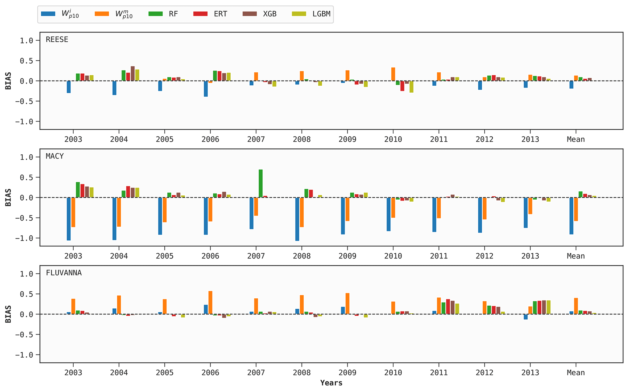
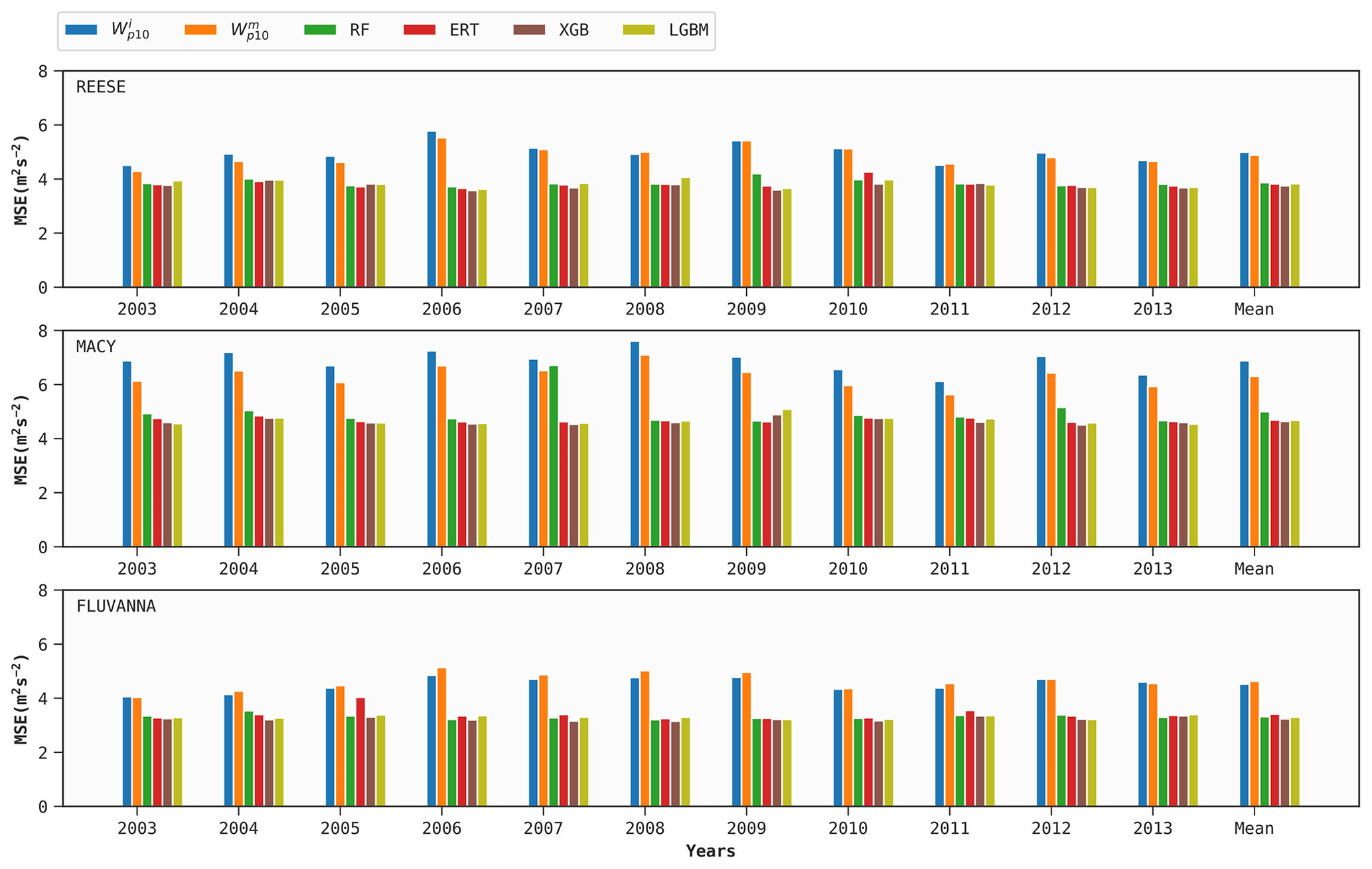
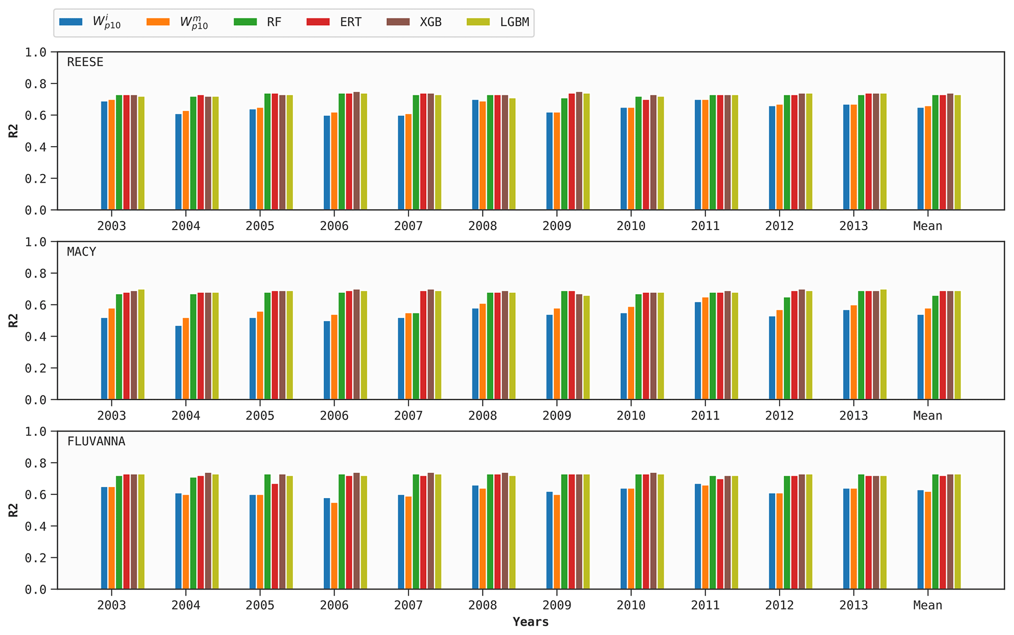
As mentioned earlier, 1 year of training data for each WTM station is used to build four DT-based models (optimized via FLAML). Out of these samples, 72 d worth of data are used for hyperparameter tuning for each case, following Sect. 6.1. These site-specific tuned models are then used to predict W_p for the other 10 years for the same site. We repeat the procedure in a round-robin manner for the other years. The mean prediction scores of all the models, in terms of the bias, MAE, MSE, and R² metrics, are given in Figs. 4–7, respectively.

Figure 4 Bias (m s⁻¹) scores of two baseline ERA5 variables and four DT-based models.

Figure 5 MAE (m s⁻¹) scores of two baseline ERA5 variables and four DT-based models.

Figure 6 MSE (m² s⁻²) scores of two baseline ERA5 variables and four DT-based models.

Figure 7 R² scores of two baseline ERA5 variables and four DT-based models.

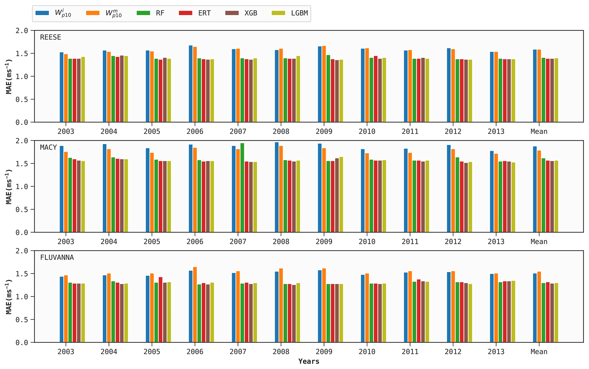
As an illustrative example, let us consider the random forest (RF) model at REESE. First, a distinct RF model is trained using data from 2003 to predict W_p for the years 2004, 2005, …, and 2013. Next, we use the data from 2004 to make predictions for the years 2003, 2005, 2006, …, and 2013. We repeat this procedure for all the possible 10 combinations. For the year 2003, the average MAE from these 10 predictions is 1.39 m s⁻¹.

According to Fig. 4, the ML models have a tendency to overestimate the wind gusts; however, the bias values are typically much lower than 0.5 m s⁻¹. The performance of the baseline predictors from ERA5 is much poorer. At MACY, both the $W_{\mathrm{p}\mathrm{10}}^{\mathrm{i}}$ and $W_{\mathrm{p}\mathrm{10}}^{\mathrm{m}}$ variables excessively underestimate wind gusts.

From Figs. 5–7, it is clear that the performance of ERA5's $W_{\mathrm{p}\mathrm{10}}^{\mathrm{i}}$ and $W_{\mathrm{p}\mathrm{10}}^{\mathrm{m}}$ variables as surrogates for W_p exhibits inter-annual variability. For example, for the $W_{\mathrm{p}\mathrm{10}}^{\mathrm{i}}$ variable, the MAE at REESE ranges from 1.53 m s⁻¹–1.68⁻¹ with an average of 1.59 m s⁻¹. These figures also attest to the superior performance of the ERA5 baseline at the REESE and FLUVANNA stations in comparison to MACY. Given the complex location of MACY and the coarse effective resolution of ERA5, such a deterioration in performance at MACY is expected.

All the performance metrics are considerably improved when using the DT-based models instead of the ERA5 baseline. According to Fig. 7, the XGB model improves the average R² scores for the REESE, MACY, and FLUVANNA stations by 0.08, 0.11, and 0.11, respectively, in comparison to the ERA5 $W_{\mathrm{p}\mathrm{10}}^{\mathrm{m}}$ baseline. The performances of the four DT-based ML models are pretty similar. In the case of REESE, the XGB model provides 12 %, 13 %, and 23 % improvements in terms of R², MAE, and MSE, respectively.

In Figs. 5–7, all the scores of the ML models are averaged over 10 years. Due to averaging, the perceived inter-annual variability in all these models is much lower in comparison to the ERA5 baseline. For example, in the context of the XGB model, the R² score at MACY has a narrow range of 0.68–0.70. In order to investigate the year-to-year variability and performance of an ML model, we report the annual R² scores at the MACY station in Table 3. As an illustrative example, we only tabulate the results of the XGB model. The results of the other ML models are very similar and, thus, are not shown. It is satisfying to see that the inter-annual variability in the R² score is not more pronounced than the ERA5 baseline. In other words, with only 1 year of training data, the XGB model can estimate W_p values for other years with R² scores ranging from 0.63 to 0.74. These scores are considerably higher than the corresponding values (R²=0.52–0.65) from the ERA5 $W_{\mathrm{p}\mathrm{10}}^{\mathrm{m}}$ baseline.

Table 3 Detailed R² scores of the XGB model at the MACY station for each year.

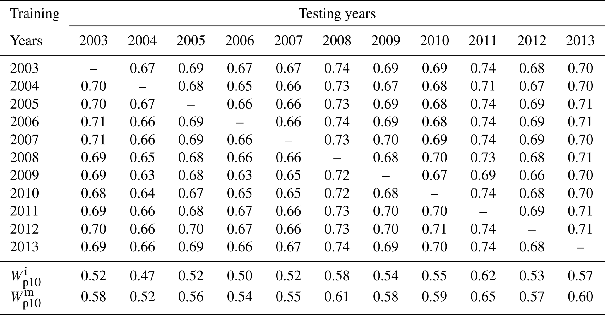
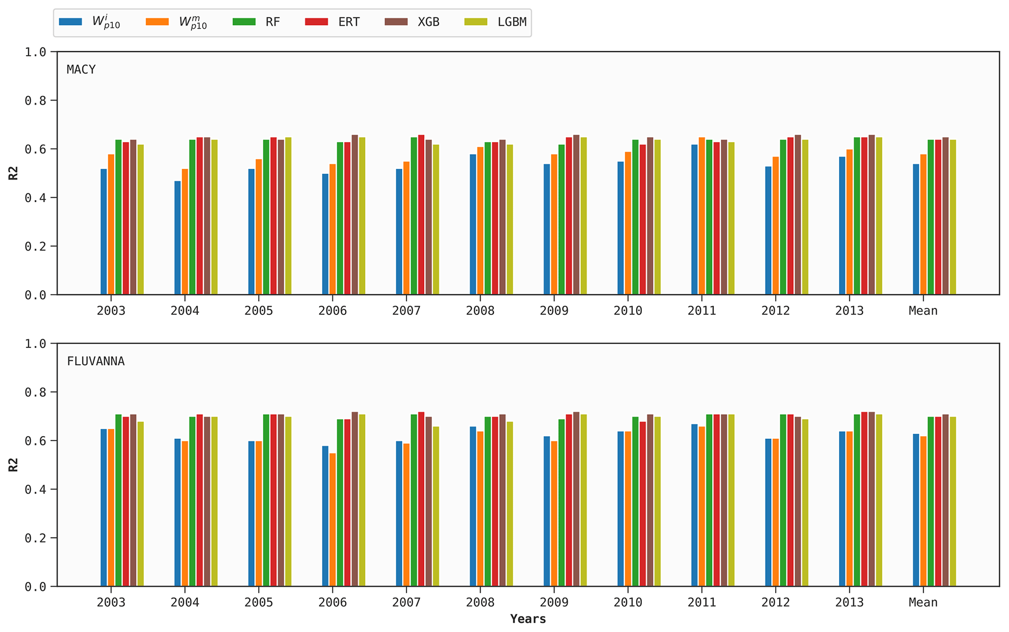
Figure 8 R² scores of the two baseline ERA5 variables and four DT-based models at MACY and FLUVANNA. Models are trained using data from the REESE station.

7.2 Cross-prediction

In order to demonstrate the potential generalizability of the ML models, the optimized models for the REESE station are utilized for predictions at the MACY and FLUVANNA stations. The R² scores are reported in Fig. 8. In the case of self-prediction, the R² scores for the ML models were around 0.66–0.69 for MACY and 0.72–0.73 for FLUVANNA (refer to Fig. 7). In the case of cross-prediction, the results are slightly poorer. In the case of MACY, the R² values are approximately equal to 0.64, whereas the corresponding R² values are around 0.70–0.71 at FLUVANNA. These results are encouraging and imply that the proposed INTRIGUE approach might be used for cross-predictions as long as the training and testing locations are not too far apart and experience similar regional climatic conditions. Along these lines, more studies are needed for rigorous validations.

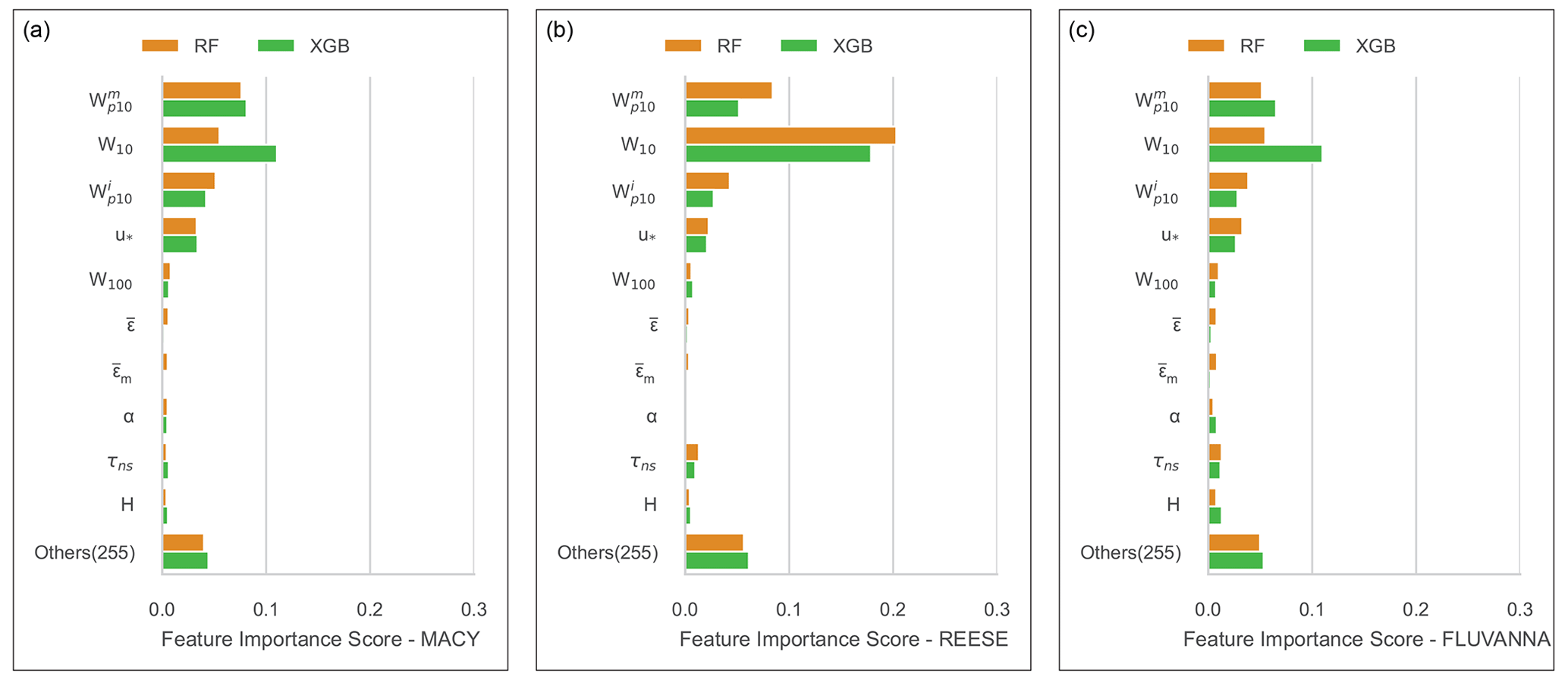
Figure 9 Feature importance scores of the ERA5 parameters for REESE (a), MACY (b), and FLUVANNA (c). The results from two ML models, XGB and RF, are shown for comparison.

7.3 Feature importance

In the INTRIGUE approach, we have used 265 input features. It is likely that not all of these features are equally important for peak wind gust predictions. One way to rank the input features is via using the “permutation feature importance” strategy (Breiman, 2001; Molnar, 2022). To describe this simple algorithm, we closely follow Sect. 7.5 of Molnar (2022).

First, an ML model (say XGB) is trained using 1 year of data from a specific station (e.g., REESE). Then, we make a prediction for another year for the same station. Both the training and testing data contain 265 input features. Using the observed and predicted W_p values, we compute prediction errors (e.g., using R²) and denote this error as e_o. Next, we randomly shuffle only one of the input features (say the ith feature) of the test data and keep the ordering of all other features the same. Now, we make a new prediction. The error associated with this new prediction is denoted as $e_{\mathrm{p}}^{\mathrm{i}}$. Since we have randomized only one input feature, that feature no longer has any association with the other input features. Thus, we expect $e_{\mathrm{p}}^{\mathrm{i}}$ to be worse than e_o; in the case of R², $e_{\mathrm{p}}^{\mathrm{i}}\le e_{\mathrm{o}}$. To achieve converged statistics, we repeat the randomization process for the same ith feature a few times (typically five or more) and compute an averaged value of $\stackrel{\mathrm{‾}}{e_{\mathrm{p}}^{\mathrm{i}}}$. The net reduction the in R² score due to the randomization of the ith feature is $\left(e_{\mathrm{o}}-\stackrel{\mathrm{‾}}{e_{\mathrm{p}}^{\mathrm{i}}}\right)$.

One at a time, we repeat the random-shuffling exercise for all 265 input features and compute the reduction in R² corresponding to each input feature. If an input feature is very important for peak wind gust estimation, the reduction in R² for that feature will be large. On the other hand, the irrelevant input features marginally impact the R² scores.

In Fig. 9, the importance (in terms of reduction in R²) of all the input features is plotted for the XGB and RF models. For computation, we use the ELI5 library (https://eli5.readthedocs.io/en/latest/overview.html, last access: 14 October 2023). We average the statistics over 10 years for robustness.

Although there are differences in the magnitude of the feature importance depending on the stations, the following input features are found to be very relevant for all three stations: W₁₀, $W_{\mathrm{p}\mathrm{10}}^{\mathrm{m}}$, $W_{\mathrm{p}\mathrm{10}}^{\mathrm{i}}$, u_*, τ_ns, W₁₀₀, $\stackrel{\mathrm{‾}}{\mathit{\epsilon }}$, ${\stackrel{\mathrm{‾}}{\mathit{\epsilon }}}_{\mathrm{m}}$, and α. Interestingly, both the XGB and RF models capture the same behavior. These input features are also the ones that are commonly used in physical parameterizations (see Sect. 2).

Some of the input features (e.g., related to the time of day, temperature, cloud cover) are not relevant for peak wind gust predictions. Thus, one can remove these input features from future ML models and achieve a similar level of prediction accuracy with reduced computational costs.

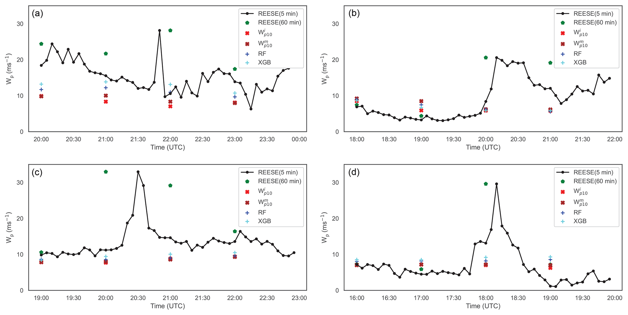
Figure 10 Examples of extreme wind gust events measured at the REESE station on 19 June 2008 (a; non-supercell thunderstorm), 14 August 2008 (b; non-supercell thunderstorm), 4 June 2009 (c; bow-echo/supercell thunderstorm), and 12 August 2009 (d; non-supercell thunderstorm). In these figures, the instantaneous ($W_{\mathrm{p}\mathrm{10}}^{\mathrm{i}}$) and mean ($W_{\mathrm{p}\mathrm{10}}^{\mathrm{m}}$) wind gust values from the ERA5 dataset are overlaid for comparison. In addition, we have plotted the predictions from the RF and XGB models.

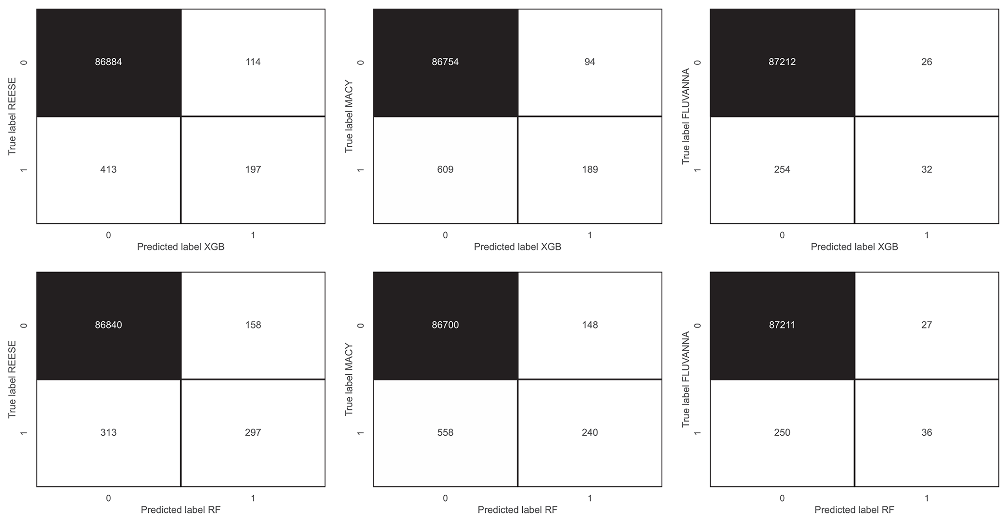
Figure 11 Confusion matrices for extreme wind gust (W_p>20 m s⁻¹) prediction. The top and bottom panels represent XGB and RF models, respectively. The left, middle, and right panels correspond to the REESE, MACY, and FLUVANNA stations, respectively.

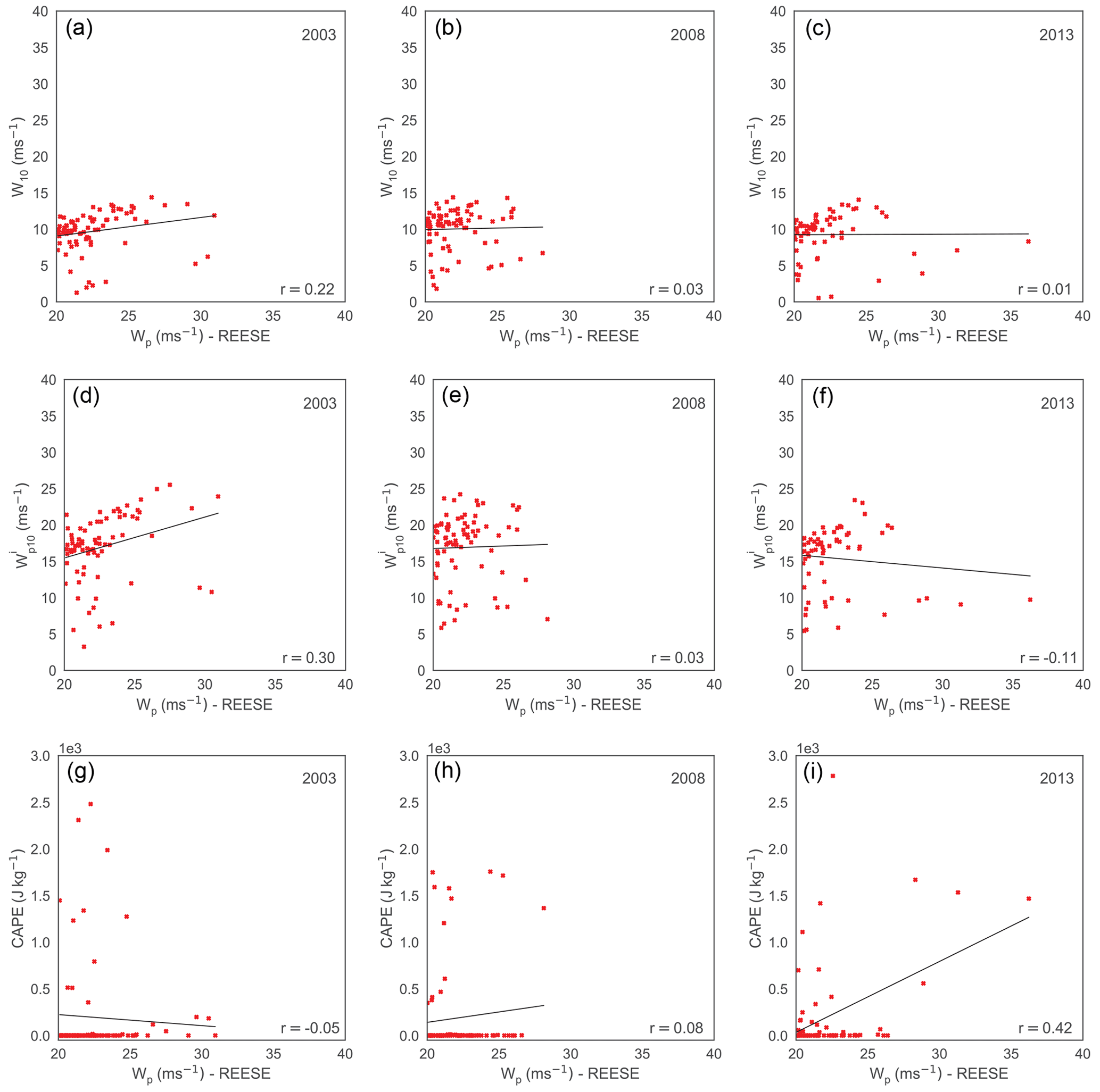
Figure 12 Scatterplots of W₁₀ (a–c), $W_{\mathrm{p}\mathrm{10}}^{\mathrm{i}}$ (d–f), and CAPE (g–i) against W_p measured at the REESE station. The W_p values greater than 20 m s⁻¹ are only included in these plots. The left, middle, and the right panels correspond to years 2003, 2008, and 2013, respectively. There are only 77, 78, and 63 samples in the left, middle, and the right panels, respectively. It is clear that the correlations between the predictors and the predictand are very low for all the cases. In the bottom-right corner of each plot, we report the Pearson's correlation coefficient (r). The black lines in these plots represent the linear regression fits.

8 Limitations of the INTRIGUE approach

The WTM dataset contains a handful of extreme wind gust events. In Fig. 10, a few illustrative cases measured at the REESE station are shown. One of these cases is related to a supercell thunderstorm, while the others are produced by non-supercell thunderstorm events. These cases and a few others were studied in depth by Lombardo et al. (2014). On these plots, we have overlaid $W_{\mathrm{p}\mathrm{10}}^{\mathrm{i}}$ values from ERA5 and also the predictions from two of the ML models (i.e., RF and XGB). It is apparent that the $W_{\mathrm{p}\mathrm{10}}^{\mathrm{i}}$ variable has not captured the extreme wind gusts in a faithful manner. This failure is likely due to the coarse effective resolution of the ERA5 data, which cannot resolve thunderstorms. The ML models are unable to make any improvement to these extreme wind gust predictions.

To further investigate this limitation of the INTRIGUE approach, we provided several confusion matrices in Fig. 11. We classified peak wind gusts into extreme (1) and nominal (0). When W_p exceeds 20 m s⁻¹, we denote the event as an extreme. From these matrices, it is evident that the INTRIGUE approach leads to numerous false positives and false negatives.

In Fig. 12, we show scatterplots of a few input features (or predictors) and the predictand (W_p). While discussing feature importance, we demonstrated that overall W₁₀, $W_{\mathrm{p}\mathrm{10}}^{\mathrm{i}}$, and $W_{\mathrm{p}\mathrm{10}}^{\mathrm{m}}$ are very important features. However, these features are barely correlated with W_p for extreme conditions. Furthermore, ERA5's CAPE variable (typically related to thunderstorm development) is also not well correlated with W_p values. In lieu of adequate input features, the INTRIGUE approach fails to perform satisfactorily for the extreme wind gust conditions. We speculate that parameters derived from vertical profiles of the ERA5 reanalysis (e.g., deep-layer wind shear, storm relative helicity, integrated Scorer parameter, Sangster parameter) as input features might improve the predictions.

In this study, we have utilized the INTRIGUE approach for W_p predictions at 10 m heights. The availability of W_p for higher altitudes is rather limited, and only a few studies (e.g., Deacon, 1955; Brook and Spillane, 1970; Suomi et al., 2015; Hu et al., 2018; Shu et al., 2021) exist in the literature. However, high-altitude (say 100 m) W_p data are highly relevant from a wind energy perspective. The contemporary physical parameterizations (see Suomi et al., 2013, and the references therein) use the surface friction velocity, sensible heat flux, and boundary layer height as input for the estimation of hub-height W_p values. Since the INTRIGUE approach already uses these input features (among others), it should be applicable for W_p predictions for turbine hub heights. Undoubtedly, more work is needed in this arena.

9 Conclusions

In this study, we proposed a decision-tree-based MCP approach (called INTRIGUE) for peak wind gust estimation. This approach utilizes several meteorological variables (including the instantaneous wind gust variable) from the ERA5 reanalysis dataset as input features. For non-extreme (i.e., nominal) cases, the INTRIGUE-approach-predicted peak wind gust values are closer to the observed ones than the baseline approaches. This approach can also make predictions for neighboring stations where training data are not available. In addition to site assessments, our proposed INTRIGUE approach can be used in wind gust forecasting. Instead of a reanalysis dataset, predicted meteorological fields from a numerical weather prediction model can be used as input features for the ML models.

However, there is room for significant improvements as the INTRIGUE approach drastically underestimates extreme wind gust events of magnitudes higher than 20 m s⁻¹. For these cases, none of the 265 input features that we considered in this study correlate with W_p. Clearly, we need more relevant input features. In our future work, we will also analyze meteorological profiles from ERA5 and compute various thunderstorm-related parameters as input features. In addition, we will add input features extracted from radar reflectivity fields using autoencoders. We speculate that the addition of such input features will enable the INTRIGUE approach to capture extreme wind gusts in a more faithful manner.

We would like to remind the readers that we intentionally use only 1 year of training data in this study. As a result, only a few such extreme cases (on the order of 60–80 samples) are included in the training process. In the ML literature, this problem is known as the imbalance data problem. In the future, we will explore various ML strategies (e.g., isolation forest) to tackle this challenging problem.

In typical wind energy projects, one does not have access to on-site long-term wind gust datasets. Thus, increasing the sample size from a single site is not a viable solution. However, it will be possible to increase the sample size by aggregating observational data from different sites around the world with comparable climatic conditions. By doing so, we will be able to come up with a more generalized ML model for wind gust prediction. We will pursue this line of research in the near future.