Analysis and multi-objective optimisation of wind turbine torque control strategies

The combined wind speed estimator and tip-speed ratio (WSE–TSR) tracking wind turbine control scheme has seen recent and increased traction from the wind industry. The modern control scheme provides a flexible trade-off between power and load objectives. On the other hand, the Kω² controller is often used based on its simplicity and steady-state optimality and is taken as a baseline here. This paper investigates the potential benefits of the WSE–TSR tracking controller compared to the baseline by analysis through a frequency-domain framework and by optimal calibration through a systematic procedure. A multi-objective optimisation problem is formulated for calibration with the conflicting objectives of power maximisation and torque fluctuation minimisation. The optimisation problem is solved by approximating the Pareto front based on the set of optimal solutions found by an explorative search. The Pareto fronts were obtained by mid-fidelity simulations with the National Renewable Energy Laboratory (NREL) 5 MW turbine under turbulent wind conditions for calibration of the baseline and for increasing fidelities of the WSE–TSR tracking controller. Optimisation results show that the WSE–TSR tracking controller does not provide further benefits in energy capture compared to the baseline Kω² controller. There is, however, a trade-off in torque control variance and power capture with control bandwidth. By lowering the bandwidth at the expense of generated power of 2 %, the torque actuation effort reduces by 80 % with respect to the optimal calibration corresponding to the highest control bandwidth.

1 Introduction

Of all the available renewable energy sources, wind energy is increasingly considered one of the most cost-effective and sustainable with regard to the global demand for clean energy (Watson et al., 2019). The total present wind power capacity installed worldwide is now 837 GW, with year-on-year growth of 12 % (Lee and Zhao, 2022). However, this growth rate must quadruple by the end of the decade to meet the net-zero emissions targets set after the Glasgow climate summit (United Nations, 2021; Komusanac et al., 2022). To achieve these ambitious climate goals in an efficient manner, the industry is developing larger turbines with a more flexible rotor assembly and support structure to exploit higher wind speeds (Veers et al., 2019). Increasingly advanced and optimised control technologies are needed to facilitate and enable the increased sizes of wind turbines (Pao and Johnson, 2011).

Variable-speed turbines usually employ a generator torque control strategy to maximise the energy capture in partial-load conditions (Bossanyi, 2000; Burton et al., 2011). Maximum power is extracted by operating the turbine at the maximum power coefficient, corresponding to a specific tip-speed ratio and pitch angle (Bottasso et al., 2012). The optimal tip-speed ratio is tracked by varying the generator torque resulting from a closed-loop controller, while the pitch angle is generally kept constant in the partial-load region (Pao and Johnson, 2011).

Nowadays, the Kω² controller is still a commonly considered partial-load region wind turbine torque control strategy due to its satisfactory performance, ease of derivation and simple implementation by only requiring a measurement of the rotor or generator speed (Johnson et al., 2006; Ozdemir et al., 2013). Nevertheless, the Kω² controller has shortcomings that can result in suboptimal power-tracking performance (Johnson et al., 2004). First, the torque gain K is calculated from modelled wind turbine properties, often subject to assumptions and estimation errors (Abbas et al., 2022). Even if the gain K is initially accurate, the turbine properties can change over time due to e.g. blade erosion and ice, dirt and/or bug buildup, thereby causing this initial value to be suboptimal (Johnson et al., 2004, 2006). For instance, according to Fingersh and Carlin (1999), a 5 % error in the optimal tip-speed ratio can lead to inaccurate K and, consequently, to a cumulative captured energy loss of 1 %–3 %. Second, suppose the wind turbine operates in turbulent wind conditions and that K is accurately determined. In this case, the large rotor inertia prevents fast acceleration and thus hinders the tracking of rapid changes in wind speed, leading to a lower operating power coefficient (Bossanyi, 2000). This problem is emphasised for heavy rotors and sharp power coefficient curves.

The torque gain K can be calibrated through an extremum seeking control (ESC) acting on the rotor power to overcome the effect of time-varying wind turbine properties (Creaby et al., 2009). While providing an energy capture improvement of 8 %–12 % when applied on the Controls Advanced Research Turbine (CART), this control scheme results in being sensitive to wind speed variations (Xiao et al., 2016). Therefore, Rotea (2017) proposes a log-of-power feedback in the ESC algorithm (LP-ESC). Using high-fidelity large-eddy simulations, Ciri et al. (2018) demonstrate that this modification renders the controller independent of changes in the mean wind speed.

One way to increase the energy capture for higher turbulence intensity is by reducing the gain K below the nominal value. This choice allows the generator torque to decrease and the rotor to accelerate more quickly in response to a gust. For instance, in the study conducted by Johnson et al. (2004), a reduction of 10 % in the gain K of the CART rotor controller resulted in a measurable increase of 0.5 % in captured power. This gain reduction strategy, aimed at enhancing energy capture, is not limited to the CART rotor alone; it holds the potential for implementation on any existing wind turbine employing the Kω² controller. It is important to note that there is no discernible linear correlation between the gain reduction factor and the specific site conditions. Consequently, it becomes evident that the extent of increased captured power is contingent upon the turbulent wind conditions and the characteristics of the particular turbine in use. Given this variability, selecting a constant value for the gain reduction factor is deemed impractical (Johnson et al., 2004).

To provide better rotor acceleration and deceleration, Fingersh and Carlin (1999) proposed the optimally tracking rotor (OTR) controller. This scheme augments the Kω² controller with a second term. The additional term is a gain multiplied by the net torque, being the difference between the (estimated) aerodynamic torque and the generator torque contribution resulting from the Kω² control law. Subtracting the new term from the original formulation will aid rotor acceleration or deceleration if the wind speed increases or decreases. With this approach applied to the CART, the controller bandwidth for tracking the actual optimal operating point is increased, thereby improving the energy capture by about 1.2 % (Fingersh and Carlin, 1999). However, the OTR control scheme relies heavily on correct knowledge of the aerodynamic rotor properties. Incorrect information will inevitably lead to suboptimal operation in transient and steady-state conditions. Another more advanced turbine controller was developed by van der Hooft et al. (2003) and includes pseudo-feedforward control based on an estimation of the rotor-effective wind speed (REWS) to realise an additional pitch control action in partial-load conditions. With this strategy, an energy yield increase of 0.9 % was achieved at the expense of larger speed and load variations.

To cope with the described disadvantages of the Kω² control scheme, combined wind speed estimator and tip-speed ratio (WSE–TSR) tracking control schemes have recently been considered (Abbas et al., 2022). The idea behind this scheme is to use the estimated REWS (Østergaard et al., 2007; Soltani et al., 2013) to calculate an estimate of the desired rotor speed, which in turn is employed as a feedback signal to close the loop by a proportional and integral (PI) controller. According to Bossanyi (2000), this controller allows for tracking the optimal tip-speed ratio even in turbulent wind conditions, with a 1 % power increase compared to the baseline Kω², but at the expense of significant power variations.

In the work of Boukhezzar and Siguerdidjane (2005), a Kalman filter estimator combined with a rotor speed reference tracking improves the power capture by 10 % when compared with the Kω² controller, but no analytical demonstration of its dynamic behaviour was provided. A similar study by Abbas et al. (2022) focused only on a time-domain analysis when comparing the combined estimator-feedback controller with the Kω² control law. Earlier work by the current authors (Brandetti et al., 2022) has proved that an analytical frequency-domain framework could be a valuable tool for analysing the dynamics of the WSE–TSR tracking controller. However, neither the performance benefits of using such a control scheme over the baseline Kω² controller nor the optimal calibration are discussed in Brandetti et al. (2022).

Therefore, this paper presents the steady-state equivalence and dynamic differences between these Kω² and WSE–TSR tracking controllers and proposes a systematic procedure for optimal calibration. Calibration of the parameters in the WSE–TSR tracking control scheme is fundamental to optimising controller performance in terms of power maximisation, load minimisation and stability (Bossanyi, 2000).

However, the use of classical analysis techniques to calibrate the proposed scheme is complex due to the trade-off between conflicting control requirements, e.g. maximising power production and minimising the loads. Recent studies (Odgaard et al., 2016; Lara et al., 2023) have demonstrated the effectiveness of multi-objective optimisation techniques based on Pareto fronts for tuning wind turbine controllers. For this reason, the calibration of the WSE–TSR tracking controller is formulated as a multi-objective optimisation problem. First, the parameter space of the considered control scheme is explored by a guided search procedure. Subsequently, the set of optimal solutions is found to construct the Pareto front in a trade-off between power maximisation and load minimisation. The solutions found are then assessed using the extended version of the frequency-domain framework, based on Brandetti et al. (2022), for comparison with the baseline controller. As also shown by Leith and Leithead (1997), analysing a controller in the frequency domain allows for gathering relevant insights into its performance. Therefore, applying a frequency-domain framework to evaluate the optimal solutions found by solving the multi-objective optimisation problem enables linking the conflicting control objectives with the stability and performance of the closed-loop system in terms of controller bandwidth.

In this context, the present research aims to illustrate the additional benefits of using the WSE–TSR tracking controller compared to the baseline Kω² for partial-load control when applied to realistic wind turbine sizes, in terms of two performance metrics widely discussed in the literature: power maximisation and load minimisation (Leith and Leithead, 1997; Leithead and Connor, 2000). Thereby, the following contributions are presented:

• demonstrating the steady-state similarities and dynamic differences between the WSE–TSR tracking control scheme and the baseline Kω² controller in the frequency domain by a universal linear analysis framework,

• mapping the performance of the fixed-structure WSE–TSR tracking controller for sets of calibration parameters of increasing dimensionality by a guided exploratory search in their constrained parameter spaces,

• formulating the optimal calibration as a multi-objective problem using Pareto front approximation techniques,

• exploiting the frequency-domain framework in conjunction with mid-fidelity simulations under realistic environmental conditions to discover and showcase the characteristics of an optimally calibrated WSE–TSR tracking control scheme to the baseline strategy.

The paper is structured as follows: Sect. 2 gives a mathematical overview of the WSE–TSR tracking control scheme and baseline Kω² controller, together with the assumptions made for their implementation. Based on the nonlinear implementation, Sect. 3 provides a linear frequency-domain framework analysing the two controllers. Section 4 illustrates the exploration and multi-objective Pareto optimisation strategy for calibrating the WSE–TSR tracking control scheme. Section 5 evaluates the performance of the calibrated WSE–TSR tracking scheme compared to the baseline controller by leveraging the results from the frequency-domain analysis framework and the ones derived from realistic mid-fidelity time-domain simulations. Finally, Sect. 6 summarises the main findings and recommendations for future work.

Prerequisites

This section provides the prerequisites needed for the analysis of the controllers. Estimated quantities and time derivatives are indicated by $\widehat{(\cdot )}$ and $\dot{(\cdot )}$, respectively. Values corresponding to a specific operating point are denoted by $\stackrel{\mathrm{‾}}{(\cdot )}$, whereas values indicating the intended optimal parameters are presented with $(\cdot {)}_{*}$. The symbols ω_r, T_g, V and λ represent the rotational speed, generator torque, wind speed and tip-speed ratio signals in the time domain, while Ω_r, 𝒯_g, 𝒱 and Λ represent the corresponding signals in the frequency domain.

In addition, this work relies on a set of assumptions, which are formulated as follows.

Assumption 1.1. The considered control schemes are analysed in the partial-load region with a constant (fine-) pitch angle. For this reason, the power coefficient mapping is only taken as a function of the tip-speed ratio.

Assumption 1.2. The generator torque control input and the rotational speed of the turbine are measured signals. The rotor-effective wind speed is considered an unknown and positive disturbance input to the plant.

Assumption 1.3. The turbine model information included in the estimator and control framework represents the actual turbine characteristics. This assumption highlights the best-case performance benefits achievable with the WSE–TSR tracking control scheme over the baseline Kω² control strategy without capturing the inherent uncertainties of real-world turbine dynamics. The assessment of the effects of model uncertainty on performance levels and control robustness is devoted to future work.

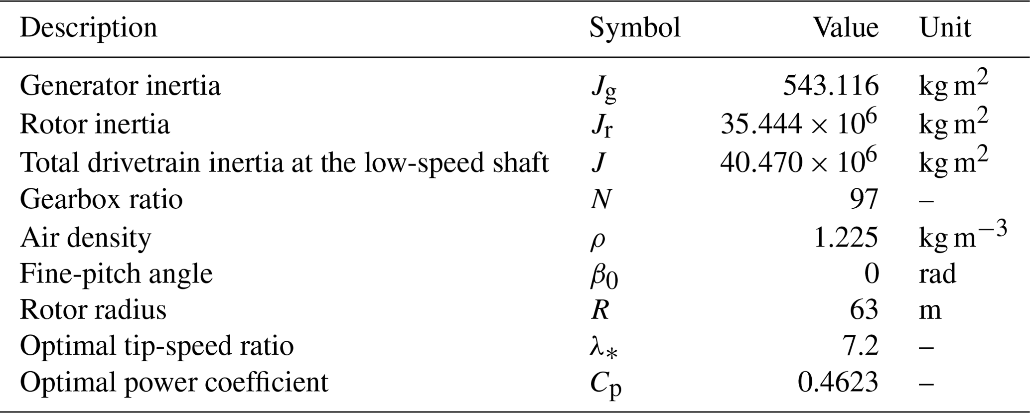
Table 1 Main operational parameters for the National Renewable Energy Laboratory (NREL) 5 MW turbine (Jonkman et al., 2009).

2 Theory of partial-load control schemes

The baseline Kω² controller is a well-known, effective and commonly used torque control strategy for maximising energy capture in the partial-load operating region (Bossanyi, 2000). While the Kω² strategy provides satisfactory performance, it is inflexible in providing a granular trade-off between power and load objectives for present-day wind turbines. Therefore, modern large-scale wind turbines are controlled by more advanced WSE–TSR tracking schemes (Mulders et al., 2023), and wind turbine manufacturers are currently exploring the possibilities of applying model predictive control (MPC) to provide such flexibility (Hovgaard et al., 2015; Pamososuryo et al., 2023). This work focuses on comparing the baseline strategy, with the first being the WSE–TSR tracking control scheme, which is also often referred to as a power coefficient C_p-tracking scheme in other works (Bossanyi, 2000). In this section, first, the Kω² and WSE–TSR tracking control schemes are derived in their full and nonlinear representations. To this end, the wind turbine system is considered, and the individual required component building blocks are obtained for completing the two schemes.

2.1 Wind turbine

The wind turbine system is represented by the first-order model:

$$\begin{array}{}\text{(1)}& J{\dot{\mathit{\omega }}}_{\mathrm{r}}=T_{\mathrm{r}}-T_{\mathrm{g}}N,\end{array}$$

where ω_r represents the rotor speed, and J is the total drivetrain inertia at the low-speed shaft (LSS) side, obtained from the relation $J=J_{\mathrm{g}}{N}^{\mathrm{2}}+J_{\mathrm{r}}$, with J_g and J_r representing the generator and rotor inertias, respectively. The gearbox ratio is defined as the transmission ratio $N={\mathit{\omega }}_{\mathrm{g}}/{\mathit{\omega }}_{\mathrm{r}}$, with ω_g representing the generator speed. The turbine is considered to be subject to a torque control input T_g∈ℝ, and, according to Assumption 1.1, the aerodynamic rotor torque is given by

$$\begin{array}{}\text{(2)}& T_{\mathrm{r}}={\displaystyle \frac{\mathrm{1}}{\mathrm{2}}}\mathit{\rho }{A}_{\mathrm{rot}}{\displaystyle \frac{V^{\mathrm{3}}}{{\mathit{\omega }}_{\mathrm{r}}}}{C}_{\mathrm{p}}\left(\mathit{\lambda }\right),\end{array}$$

where ρ represents the air density; A_rot is the rotor-swept area; V∈ℝ is the rotor-effective wind speed (REWS); and C_p(⋅) is the power coefficient, being a function of the tip-speed ratio

$$\begin{array}{}\text{(3)}& \mathit{\lambda }={\displaystyle \frac{{\mathit{\omega }}_{\mathrm{r}}R}{V}},\end{array}$$

with R being the rotor radius. The shape of the C_p(⋅) curve depends on the design of the turbine and can be computed from either numerical simulations or experimental data.

This study focuses on showing the potential benefits of an advanced controller for large-scale turbines at both onshore and offshore locations. Therefore, for its size and rated power capacity, the National Renewable Energy Laboratory (NREL) 5 MW wind turbine model (Jonkman et al., 2009) is used to strike a balance. The main operational parameters are summarised in Table 1, and the C_p(⋅) curve covering the operating region of interest is illustrated in Fig. 1. The presented curve is obtained from steady-state wind turbine simulations for a wind profile with a uniform velocity of 9 m s⁻¹. It can be observed that a single λ_* exists, which corresponds to the rotor operating point for maximum power extraction efficiency $C_{\mathrm{p},*}\left({\mathit{\lambda }}_{*}\right)$. In the remainder of this paper, a distinction is made between the torque controller input variable for the two schemes, namely T_g,K and T_g,TSR, for the baseline Kω² and WSE–TSR tracking controller, respectively.

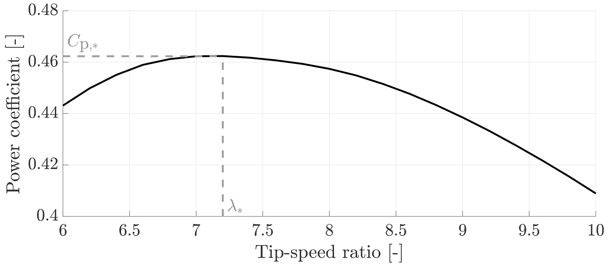
Figure 1 Power coefficient for the NREL 5 MW wind turbine model (Jonkman et al., 2009) at a uniform wind speed of 9 m s⁻¹. The maximum power extraction efficiency and the corresponding optimal tip-speed ratio are indicated as $C_{\mathrm{p},*}$ and λ_*, respectively.

2.2 Baseline Kω² controller

The derivation of the baseline Kω² control law is presented in this section. Figure 2 illustrates a block diagram of the controller, and as shown, the framework only consists of the wind turbine and the controller. The controller is a static (nonlinear) function without dynamics, providing the generator torque control signal based on the rotor speed:

$$\begin{array}{}\text{(4)}& T_{\mathrm{g},\mathrm{K}}=K{\displaystyle \frac{{\mathit{\omega }}_{\mathrm{r}}^{\mathrm{2}}}{N}},\end{array}$$

in which the torque gain K (Bossanyi, 2000) is defined at the LSS side of the drivetrain as

$$\begin{array}{}\text{(5)}& K={\displaystyle \frac{\mathit{\rho }{A}_{\mathrm{rot}}{R}^{\mathrm{3}}{C}_{\mathrm{p},*}\left({\mathit{\lambda }}_{*}\right)}{\mathrm{2}{\mathit{\lambda }}_{*}^{\mathrm{3}}}}\end{array}$$

under Assumption 1.1.

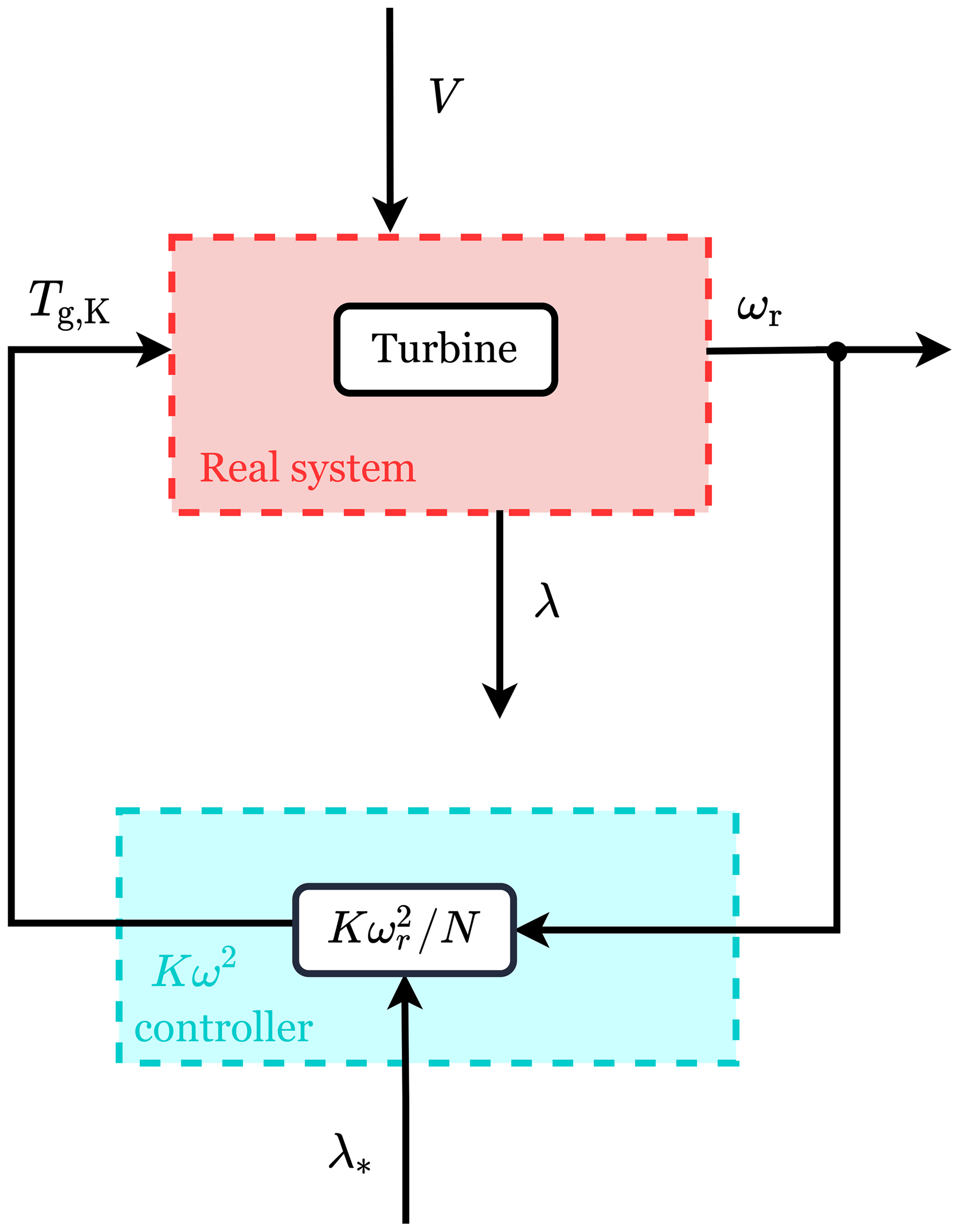
Figure 2 Block diagram of the Kω² control framework. The red box highlights the wind turbine system with two inputs (the generator torque, T_g,K, and the wind speed, V) and two outputs (the rotational speed, ω_r, and the TSR, λ). The measured ω_r and the optimal TSR, λ_*, are used as inputs of the controller (cyan box) to compute T_g,K.

2.3 WSE–TSR tracking controller

The WSE–TSR tracking framework, outlined in Fig. 3, combines an estimator and a tip-speed ratio tracking controller. The estimator provides the tip-speed ratio estimate $\widehat{\mathit{\lambda }}$, which is used by the controller that acts on the difference between the estimate and the tip-speed ratio reference. This reference is usually taken as λ_*, corresponding to the rotor operating point for maximum power extraction efficiency $C_{\mathrm{p}}^{*}$. The controller provides the torque control signal T_g,TSR and forces the turbine to track the reference. The following section provides derivations of commonly used implementations for both elements in the WSE–TSR tracking framework.

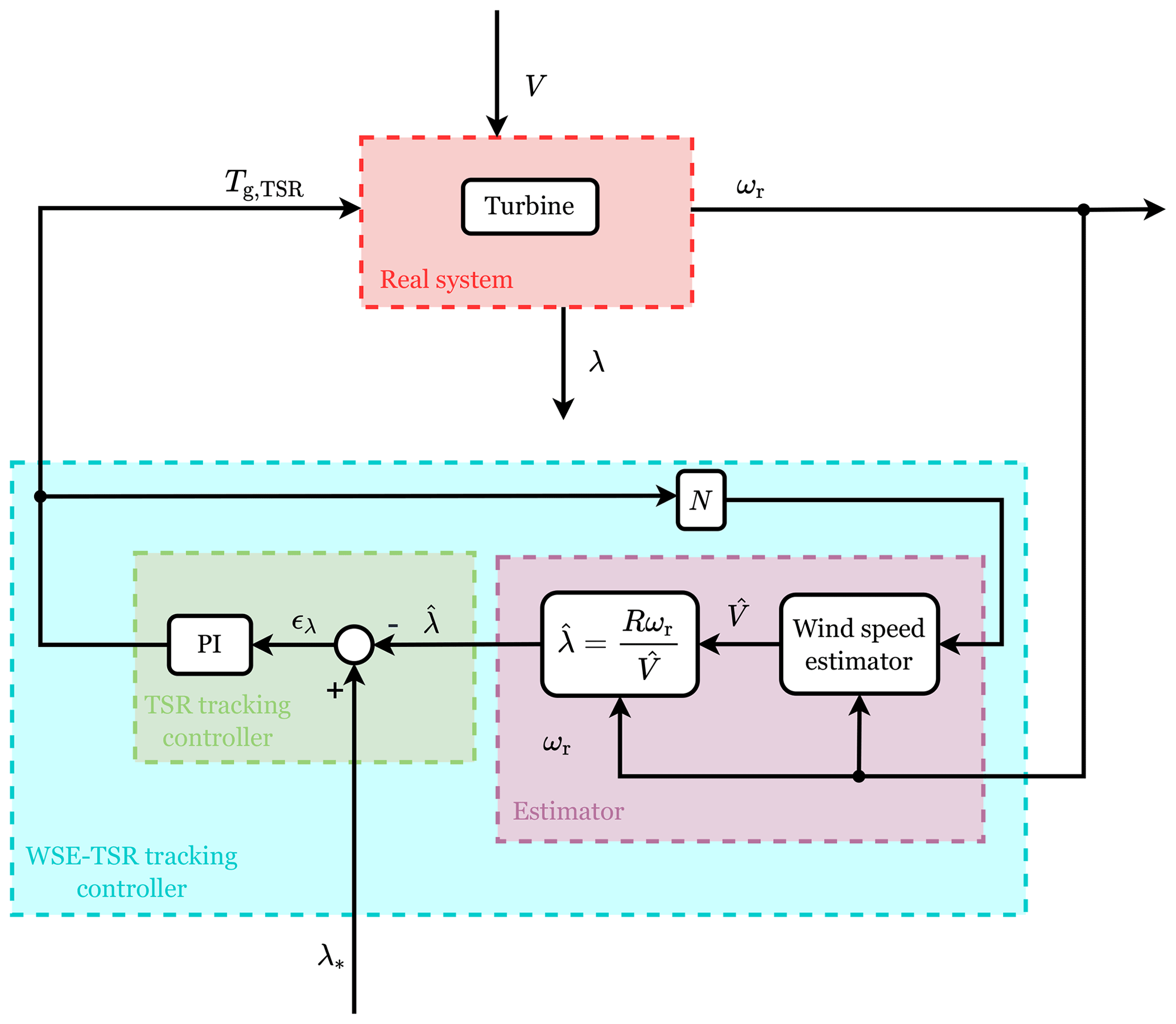
Figure 3 Block diagram of the WSE–TSR tracking control framework. The red box highlights the wind turbine system with two inputs (the generator torque, T_g,TSR, and the wind speed, V) and two outputs (the rotational speed, ω_r, and the TSR, λ). The cyan box highlights the WSE–TSR tracking controller, which includes the estimator (purple box) and the TSR tracker controller (green box). The measured T_g,TSR and ω_r are used to estimate the rotor-effective wind speed $\widehat{V}$ and to calculate an estimate of TSR, $\widehat{\mathit{\lambda }}$, in the estimator block. The controller acts on the difference between $\widehat{\mathit{\lambda }}$ and the optimal TSR, λ_*, to calculate the torque control signal T_g,TSR.

2.3.1 Wind speed estimator

The REWS is estimated based on the immersion and invariance (I&I) estimator (Ortega et al., 2013) with an augmented integral correction term (Liu et al., 2022). The estimator is illustrated in Fig. 4 and uses the control signal, the measured system plant output and a nonlinear plant model to estimate the REWS. Given Assumptions 1.2 and 1.3, the estimator is formulated as follows:

$$\begin{array}{}\text{(6)}& \left\{\begin{array}{l}J{\widehat{\dot{\mathit{\omega }}}}_{\mathrm{r}}={\widehat{T}}_{\mathrm{r}}-T_{\mathrm{g},\mathrm{TSR}}N\\ {\mathit{ϵ}}_{{\mathit{\omega }}_{\mathrm{r}}}={\mathit{\omega }}_{\mathrm{r}}-{\widehat{\mathit{\omega }}}_{\mathrm{r}}\\ \widehat{V}=K_{\mathrm{p},\mathrm{w}}{\mathit{ϵ}}_{{\mathit{\omega }}_{\mathrm{r}}}+K_{\mathrm{i},\mathrm{w}}\underset{\mathrm{0}}{\overset{t}{\int }}{\mathit{ϵ}}_{{\mathit{\omega }}_{\mathrm{r}}}\left(\mathit{\tau }\right)\mathrm{d}\mathit{\tau },\end{array}\right.\end{array}$$

with $\widehat{V}$ indicating the estimated REWS, K_p,w the proportional estimator gain and K_i,w the integral estimator gain. Furthermore, t indicates the present time, and τ is the variable of integration. By adding integral action to the estimator, the error ${\mathit{ϵ}}_{{\mathit{\omega }}_{\mathrm{r}}}$ is forced to converge to 0, providing consistent estimates of the rotor speed state ${\widehat{\mathit{\omega }}}_{\mathrm{r}}$. Under Assumption 1.1, the estimated aerodynamic torque is defined as

$$\begin{array}{}\text{(7)}& {\widehat{T}}_{\mathrm{r}}={\displaystyle \frac{\mathrm{1}}{\mathrm{2}}}\mathit{\rho }{A}_{\mathrm{rot}}{\displaystyle \frac{{\widehat{V}}^{\mathrm{3}}}{{\mathit{\omega }}_{\mathrm{r}}}}{\widehat{C}}_{\mathrm{p}}\left(\widehat{\mathit{\lambda }}\right),\end{array}$$

where ${\widehat{C}}_{\mathrm{p}}(\cdot )$ is the estimated power coefficient, being a nonlinear function of the estimated tip-speed ratio $\widehat{\mathit{\lambda }}={\mathit{\omega }}_{\mathrm{r}}R/\widehat{V}$.

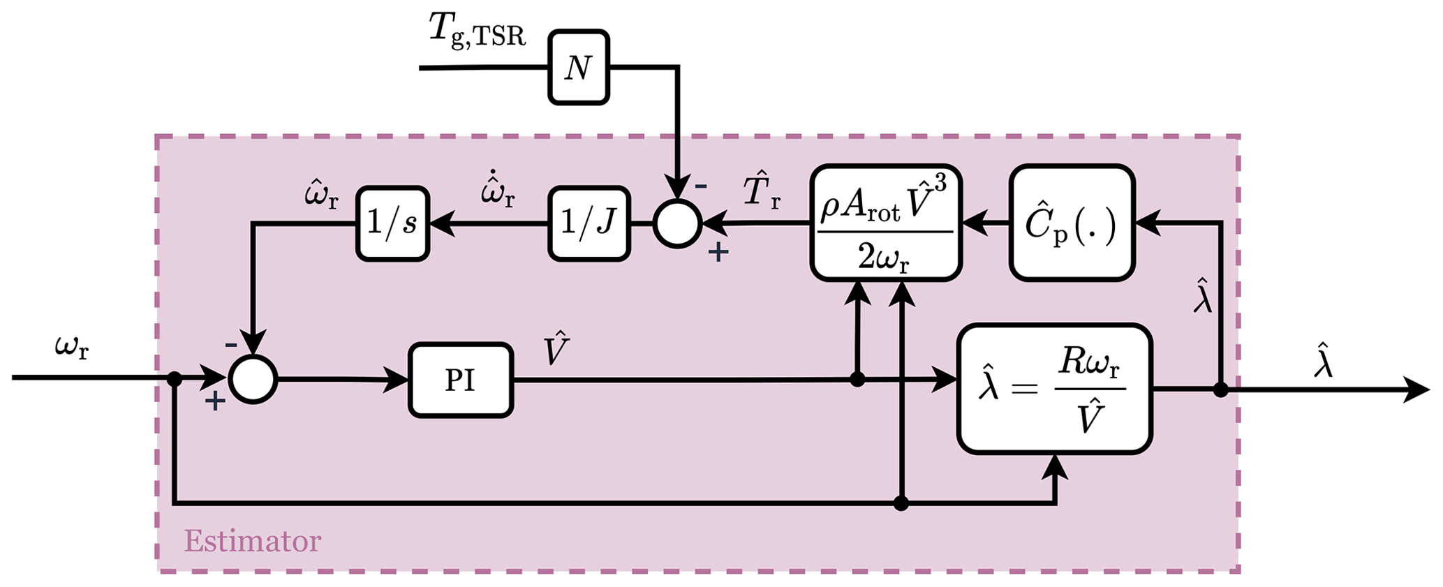
Figure 4 Block diagram of the estimator (Liu et al., 2022; Ortega et al., 2013). The measured generator torque, T_g,TSR, and rotational speed, ω_r, are used to estimate the REWS, $\widehat{V}$, and to calculate an estimate of the TSR, $\widehat{\mathit{\lambda }}$.

2.3.2 Tip-speed ratio tracking controller

The proportional and integral (PI) controller in the WSE–TSR tracking scheme acts on the tip-speed ratio error, which is defined as

$$\begin{array}{}\text{(8)}& {\mathit{ϵ}}_{\mathit{\lambda }}={\mathit{\lambda }}_{*}-\widehat{\mathit{\lambda }},\end{array}$$

being the difference between the reference and estimated tip-speed ratio. This error is used to compute the generator torque demand:

$$\begin{array}{}\text{(9)}& T_{\mathrm{g},\mathrm{TSR}}=K_{\mathrm{p},\mathrm{c}}{\mathit{ϵ}}_{\mathit{\lambda }}+K_{\mathrm{i},\mathrm{c}}\underset{\mathrm{0}}{\overset{t}{\int }}{\mathit{ϵ}}_{\mathit{\lambda }}\left(\mathit{\tau }\right)\mathrm{d}\mathit{\tau },\end{array}$$

where K_p,c and K_i,c are the respective proportional and integral controller gains.

3 Frequency-domain framework

This section provides the linear frequency-domain framework for analysing the baseline Kω² and the WSE–TSR tracking controllers, where the dynamics of the nonlinear system are linearised around a specific operating point. The subscripts (⋅)_K and (⋅)_TSR are employed to distinguish the transfer functions for the two schemes. Following the structure of Sect. 2 and in the subsequent subsections, the relevant transfer functions are first derived and provided for the wind turbine dynamics, followed by the individual and combined subsystems for the considered control schemes.

The presented framework has undergone rigorous verification procedures. Firstly, it was validated through linearisation of the fully coupled and nonlinear system, using a numerical control system linearisation tool (The MathWorks Inc., 2021). This initial step ensured the accuracy and reliability of our framework. Its correctness is further validated by comparison to the linearisation results for the same coupled system in related published work (Mulders et al., 2023). To ensure the applicability of the framework in real-world scenarios, extensive time-domain simulations of the nonlinear model were conducted using the mid-fidelity software OpenFAST (NREL, 2021). These simulations provide empirical evidence of the effectiveness of the framework in capturing system dynamics. It is important to note that, in the interest of brevity and focus, the detailed verification process is not included in this paper.

3.1 Wind turbine dynamics

This section considers the linearisation of the wind turbine dynamics. The differential equation in Eq. (1) is first combined with the nonlinear expression for the aerodynamic rotor torque defined in Eq. (2). Subsequently, the resulting expression is linearised with respect to the rotor speed state, generator torque control input and wind speed disturbance input, resulting in

$$\begin{array}{}\text{(10)}& {\dot{\mathit{\omega }}}_{\mathrm{r}}=G\left(V\right){\mathit{\omega }}_{\mathrm{r}}+E{T}_{\mathrm{g}}+H\left(V\right)V.\end{array}$$

For reasons of conciseness, the values perturbed around their operating points are defined using the same original variables. The introduced variables representing partial derivatives are defined as

$$\begin{array}{}\text{(11)}& \begin{array}{rl}G\left(V\right)& ={\displaystyle \frac{\mathrm{1}}{J}}{\displaystyle \frac{\partial T_{\mathrm{r}}}{\partial {\mathit{\omega }}_{\mathrm{r}}}}{|}_{\left({\stackrel{\mathrm{‾}}{\mathit{\omega }}}_{\mathrm{r}},\stackrel{\mathrm{‾}}{V}\right)}={\displaystyle \frac{\mathrm{1}}{\mathrm{2}J}}\mathit{\rho }{A}_{\mathrm{rot}}\left(-{\displaystyle \frac{V^{\mathrm{3}}}{{\mathit{\omega }}_{\mathrm{r}}^{\mathrm{2}}}}{C}_{\mathrm{p}}\left({\mathit{\omega }}_{\mathrm{r}},V\right)\right.\\ & \left.+{\displaystyle \frac{V^{\mathrm{2}}R}{{\mathit{\omega }}_{\mathrm{r}}}}{\displaystyle \frac{\partial C_{\mathrm{p}}\left({\mathit{\omega }}_{\mathrm{r}},V\right)}{\partial \mathit{\lambda }}}\right){|}_{\left({\stackrel{\mathrm{‾}}{\mathit{\omega }}}_{\mathrm{r}},\stackrel{\mathrm{‾}}{V}\right)},E=-{\displaystyle \frac{N}{J}},\end{array}\end{array}$$

$$\begin{array}{}\text{(12)}& \begin{array}{rl}H\left(V\right)& ={\displaystyle \frac{\mathrm{1}}{J}}{\displaystyle \frac{\partial T_{\mathrm{r}}}{\partial V}}{|}_{\left({\stackrel{\mathrm{‾}}{\mathit{\omega }}}_{\mathrm{r}},\stackrel{\mathrm{‾}}{V}\right)}={\displaystyle \frac{\mathrm{1}}{\mathrm{2}J}}\mathit{\rho }{A}_{\mathrm{rot}}\left({\displaystyle \frac{\mathrm{3}{V}^{\mathrm{2}}}{{\mathit{\omega }}_{\mathrm{r}}}}{C}_{\mathrm{p}}\left({\mathit{\omega }}_{\mathrm{r}},V\right)\right.\\ & \left.-VR{\displaystyle \frac{\partial C_{\mathrm{p}}\left({\mathit{\omega }}_{\mathrm{r}},V\right)}{\partial \mathit{\lambda }}}\right){|}_{\left({\stackrel{\mathrm{‾}}{\mathit{\omega }}}_{\mathrm{r}},\stackrel{\mathrm{‾}}{V}\right)}.\end{array}\end{array}$$

The argument V is included here to allow for the convenient definition of estimator-based expressions for G and H in a later section; however, the argument is omitted in expressions from this point onwards. Finally, the linearised expression is Laplace transformed to obtain the following:

$$(s-G){\mathrm{\Omega }}_{\mathrm{r}}\left(s\right)=E{\mathcal{T}}_{\mathrm{g}}\left(s\right)+H\mathcal{V}\left(s\right),$$

where s represents the Laplace operator. The resulting equation is defined to give the rotor speed,

$$\begin{array}{}\text{(13)}& {\mathrm{\Omega }}_{\mathrm{r}}\left(s\right)={\displaystyle \frac{E}{s-G}}{\mathcal{T}}_{\mathrm{g}}\left(s\right)+{\displaystyle \frac{H}{s-G}}\mathcal{V}\left(s\right),\end{array}$$

which depends on the transfer functions from the generator torque control and wind speed disturbance.

3.2 Analysis framework

To compare the characteristics of the baseline Kω² and WSE–TSR tracking control strategies, a universal analysis framework is defined in this section and is illustrated in Fig. 5. Here, the controllers are generalised as a single block with two inputs and one output, being the reference tip-speed ratio, rotor speed and generator torque control signals, respectively. In the linear- and frequency-domain formulation, the control scheme is formalised as

$$\begin{array}{}\text{(14)}& {\mathcal{T}}_{\mathrm{g}}\left(s\right)=K_{{\mathrm{\Omega }}_{\mathrm{r}}\to {\mathcal{T}}_{\mathrm{g}}}\left(s\right){\mathrm{\Omega }}_{\mathrm{r}}\left(s\right)+K_{{\mathrm{\Lambda }}_{*}\to {\mathcal{T}}_{\mathrm{g}}}\left(s\right){\mathrm{\Lambda }}_{*}\left(s\right).\end{array}$$

In the remainder of this section, the expressions $K_{{\mathrm{\Omega }}_{\mathrm{r}}\to {\mathcal{T}}_{\mathrm{g}}}$ and $K_{{\mathrm{\Lambda }}_{*}\to {\mathcal{T}}_{\mathrm{g}}}$ are derived and analysed for the different controllers, representing the feedback and the reference shaping terms, respectively. In particular, it will be shown that for the Kω² controller, these elements are equivalent to a state feedback controller with reference shaping gain. Since both the WSE–TSR tracking controller and a state feedback controller aim to regulate the output of the wind turbine, ω_r, so that it tracks the reference input, λ_*, this equivalence represents the first step to comparing the baseline with the proposed controller.

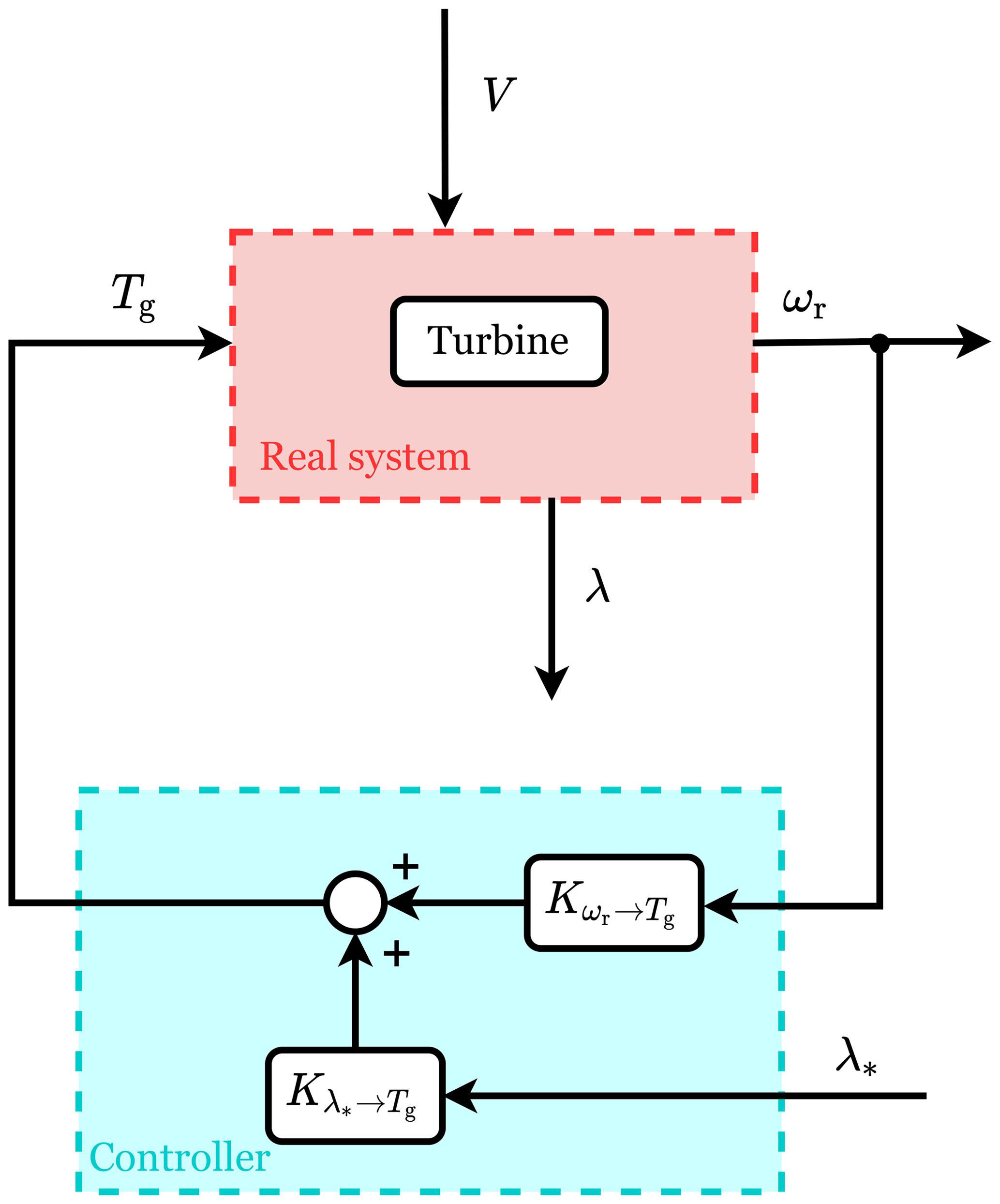
Figure 5 Block diagram of the universal framework used for the controller analysis. The red box highlights the wind turbine system with two inputs (the generator torque, T_g, and the wind speed, V) and two outputs (the rotational speed, ω_r, and the TSR, λ). The cyan box represents the controller with two inputs (ω_r and the TSR set point, λ_*), one output (T_g) and two terms used for the linear analysis framework (the feedback term, $K_{{\mathit{\omega }}_{\mathrm{r}}\to T_{\mathrm{g}}}$, and the reference shaping term, $K_{{\mathit{\lambda }}_{*}\to T_{\mathrm{g}}}$).

By substituting Eq. (14) into Eq. (13), the following expression is obtained:

$$\begin{array}{}\text{(15)}& \begin{array}{rl}{\mathrm{\Omega }}_{\mathrm{r}}\left(s\right)& ={\displaystyle \frac{E{K}_{{\mathrm{\Omega }}_{\mathrm{r}}\to {\mathcal{T}}_{\mathrm{g}}}\left(s\right)}{s-G}}{\mathrm{\Omega }}_{\mathrm{r}}\left(s\right)+{\displaystyle \frac{E{K}_{{\mathrm{\Lambda }}_{*}\to {\mathcal{T}}_{\mathrm{g}}}\left(s\right)}{s-G}}{\mathrm{\Lambda }}_{*}\left(s\right)\\ & +{\displaystyle \frac{H}{s-G}}\mathcal{V}\left(s\right),\end{array}\end{array}$$

and by further manipulation,

$$\begin{array}{}\text{(16)}& \begin{array}{rl}{\mathrm{\Omega }}_{\mathrm{r}}\left(s\right)& ={\displaystyle \frac{E{K}_{{\mathrm{\Lambda }}_{*}\to {\mathcal{T}}_{\mathrm{g}}}\left(s\right)}{s-G-E{K}_{{\mathrm{\Omega }}_{\mathrm{r}}\to {\mathcal{T}}_{\mathrm{g}}}\left(s\right)}}{\mathrm{\Lambda }}_{*}\left(s\right)\\ & +{\displaystyle \frac{H}{s-G-E{K}_{{\mathrm{\Omega }}_{\mathrm{r}}\to {\mathcal{T}}_{\mathrm{g}}}\left(s\right)}}\mathcal{V}\left(s\right).\end{array}\end{array}$$

In Eq. (16), the closed-loop transfer functions are defined with the rotor speed as the output variable. As the scheme intends to regulate the tip-speed ratio to the TSR reference, this output should be converted to the actual tip-speed ratio λ of the turbine rotor. Therefore, the TSR expression defined in Eq. (3) is linearised with respect to the rotor speed and wind speed, and the following expression is obtained:

$$\begin{array}{}\text{(17)}& \mathrm{\Lambda }\left(s\right)={\displaystyle \frac{R}{\stackrel{\mathrm{‾}}{V}}}{\mathrm{\Omega }}_{\mathrm{r}}\left(s\right)-{\displaystyle \frac{R{\stackrel{\mathrm{‾}}{\mathit{\omega }}}_{\mathrm{r}}}{{\stackrel{\mathrm{‾}}{V}}^{\mathrm{2}}}}\mathcal{V}\left(s\right).\end{array}$$

By combining Eq. (17) with Eq. (16),

$$\begin{array}{}\text{(18)}& \begin{array}{rl}\mathrm{\Lambda }\left(s\right)& =\underset{T_{{\mathrm{\Lambda }}_{*}\to \mathrm{\Lambda }}\left(s\right)}{\underbrace{{\displaystyle \frac{RE{K}_{{\mathrm{\Lambda }}_{*}\to {\mathcal{T}}_{\mathrm{g}}}\left(s\right)}{\stackrel{\mathrm{‾}}{V}\left(s-G-E{K}_{{\mathrm{\Omega }}_{\mathrm{r}}\to {\mathcal{T}}_{\mathrm{g}}}\left(s\right)\right)}}}}{\mathrm{\Lambda }}_{*}\left(s\right)\\ & +\underset{T_{\mathcal{V}\to \mathrm{\Lambda }}\left(s\right)}{\underbrace{{\displaystyle \frac{R\left(H-\left({\stackrel{\mathrm{‾}}{\mathit{\omega }}}_{\mathrm{r}}/\stackrel{\mathrm{‾}}{V}\right)\left(s-G-E{K}_{{\mathrm{\Omega }}_{\mathrm{r}}\to {\mathcal{T}}_{\mathrm{g}}}\left(s\right)\right)\right)}{\stackrel{\mathrm{‾}}{V}\left(s-G-E{K}_{{\mathrm{\Omega }}_{\mathrm{r}}\to {\mathcal{T}}_{\mathrm{g}}}\left(s\right)\right)}}}}\mathcal{V}\left(s\right).\end{array}\end{array}$$

The two transfer function terms on the right-hand side of Eq. (18) represent the closed-loop system reference tracking and disturbance attenuation capabilities, respectively. In particular, the term $T_{{\mathrm{\Lambda }}_{*}\to \mathrm{\Lambda }}\left(s\right)$ indicates if the controller is tracking the optimal condition (i.e. $\mathit{\lambda }={\mathit{\lambda }}_{*}$), while T_𝒱→Λ(s) shows the controller's performance in reacting to external wind speed disturbances. Later in this paper, these closed-loop transfer functions are evaluated in terms of optimal controller calibration to further investigate the controller in the frequency domain.

3.3 Baseline Kω² control dynamics

With the open-loop linearised wind turbine plant dynamics and analysis framework defined, this section derives the respective quantities in the universal controller framework for the baseline controller. The nonlinear representation of the Kω² controller given by Eq. (4) is linearised to obtain the following quantities:

$$\begin{array}{}\text{(19)}& {\displaystyle }\begin{array}{rl}{K}_{\left({\mathrm{\Omega }}_{\mathrm{r}}\to {\mathcal{T}}_{\mathrm{g}}\right),K}& ={\displaystyle \frac{\partial T_{\mathrm{g},\mathrm{K}}}{\partial {\mathit{\omega }}_{\mathrm{r}}}}{|}_{\left({\stackrel{\mathrm{‾}}{\mathit{\omega }}}_{\mathrm{r}},{\mathit{\lambda }}_{*}\right)}={\displaystyle \frac{\mathrm{2}K{\stackrel{\mathrm{‾}}{\mathit{\omega }}}_{\mathrm{r}}}{N}}\\ & ={\displaystyle \frac{\mathit{\rho }{R}^{\mathrm{3}}{A}_{\mathrm{rot}}{C}_{\mathrm{p},*}\left({\mathit{\lambda }}_{*}\right)}{N{\mathit{\lambda }}_{*}^{\mathrm{3}}}}{\stackrel{\mathrm{‾}}{\mathit{\omega }}}_{\mathrm{r}},\end{array}\text{(20)}& {\displaystyle }\begin{array}{rl}{K}_{\left({\mathrm{\Lambda }}_{*}\to {\mathcal{T}}_{\mathrm{g}}\right),K}=& {\displaystyle \frac{\partial T_{\mathrm{g},\mathrm{K}}}{\partial {\mathit{\lambda }}_{*}}}{|}_{\left({\stackrel{\mathrm{‾}}{\mathit{\omega }}}_{\mathrm{r}},{\mathit{\lambda }}_{*}\right)}={\displaystyle \frac{\mathit{\rho }{R}^{\mathrm{3}}{A}_{\mathrm{rot}}}{\mathrm{2}N}}\\ & \left(-{\displaystyle \frac{\mathrm{3}}{{\mathit{\lambda }}_{*}^{\mathrm{4}}}}{C}_{\mathrm{p},*}\left({\mathit{\lambda }}_{*}\right)+{\displaystyle \frac{\mathrm{1}}{{\mathit{\lambda }}_{*}^{\mathrm{3}}}}{\displaystyle \frac{\partial C_{\mathrm{p},*}\left({\mathit{\lambda }}_{*}\right)}{\partial {\mathit{\lambda }}_{*}}}\right){\stackrel{\mathrm{‾}}{\mathit{\omega }}}_{\mathrm{r}}^{\mathrm{2}}.\end{array}\end{array}$$

These are equivalent to the state feedback and reference shaping gain, respectively, as defined in state feedback control theory. The interested reader is referred to Sect. A for the full derivation of this similarity.

3.4 WSE–TSR tracking control dynamics

This section provides a derivation of the frequency-domain control dynamics of the WSE–TSR tracking controller. As shown in Fig. 3, the control scheme consists of a combined estimator and tracking controller. For this reason, to obtain the dynamics of the full scheme, the linear frequency-domain representations of the individual estimator and controller are derived first. Then, the framework dynamics are achieved by coupling the estimator and the controller.

3.4.1 Estimator dynamics

As illustrated in Fig. 4, the estimator has the generator torque and the rotor speed as inputs and the estimated tip-speed ratio as output. Therefore, several steps must be taken to derive a frequency-domain representation for the estimator, which are briefly summarised here. First, the equations for the estimated rotor speed and REWS (Eq. 6) are combined and applied at the linearisation point in terms of the Laplace variable. As a result, the estimated REWS is defined as a function of the rotor speed and the generator torque. Then, by substituting this expression into the nonlinear function of the estimated tip-speed ratio, the following is obtained:

$$\begin{array}{}\text{(21)}& \widehat{\mathrm{\Lambda }}\left(s\right)=X\left(s\right){\mathcal{T}}_{\mathrm{g},\mathrm{TSR}}\left(s\right)+Y\left(s\right){\mathrm{\Omega }}_{\mathrm{r}}\left(s\right),\end{array}$$

where

$$\begin{array}{}\text{(22)}& X\left(s\right)={\displaystyle \frac{{\widehat{\mathrm{\Lambda }}}_{{\mathcal{T}}_{\mathrm{g},\mathrm{TSR}}}\left(s\right)}{{\mathcal{T}}_{\mathrm{g},\mathrm{TSR}}\left(s\right)}}={\displaystyle \frac{R{\stackrel{\mathrm{‾}}{\mathit{\omega }}}_{\mathrm{r}}E\left(K_{\mathrm{p},\mathrm{w}}s+K_{\mathrm{i},\mathrm{w}}\right)}{{\stackrel{\mathrm{‾}}{V}}^{\mathrm{2}}\left(s^{\mathrm{2}}+\widehat{H}{K}_{\mathrm{p},\mathrm{w}}s+\widehat{H}{K}_{\mathrm{i},\mathrm{w}}\right)}}\end{array}$$

and

$$\begin{array}{}\text{(23)}& \begin{array}{rl}& Y\left(s\right)={\displaystyle \frac{{\widehat{\mathrm{\Lambda }}}_{{\mathrm{\Omega }}_{\mathrm{r}}}\left(s\right)}{{\mathrm{\Omega }}_{\mathrm{r}}\left(s\right)}}=\\ & {\displaystyle \frac{R\left[\left(\mathrm{1}-\left({\stackrel{\mathrm{‾}}{\mathit{\omega }}}_{\mathrm{r}}/\stackrel{\mathrm{‾}}{V}\right)K_{\mathrm{p},\mathrm{w}}\right)s^{\mathrm{2}}+\left(\widehat{H}{K}_{\mathrm{p},\mathrm{w}}-\left({\stackrel{\mathrm{‾}}{\mathit{\omega }}}_{\mathrm{r}}/\stackrel{\mathrm{‾}}{V}\right)\left(K_{\mathrm{i},\mathrm{w}}-\widehat{G}{K}_{\mathrm{p},\mathrm{w}}\right)\right)s+\left(\widehat{H}+\left({\stackrel{\mathrm{‾}}{\mathit{\omega }}}_{\mathrm{r}}/\stackrel{\mathrm{‾}}{V}\right)\widehat{G}\right)K_{\mathrm{i},\mathrm{w}}\right]}{\stackrel{\mathrm{‾}}{V}\left(s^{\mathrm{2}}+\widehat{H}{K}_{\mathrm{p},\mathrm{w}}s+\widehat{H}{K}_{\mathrm{i},\mathrm{w}}\right)}}\end{array}\end{array}$$

represent the transfer functions from the generator torque and rotational speed, respectively, to the estimated tip-speed ratio. According to Assumption 1.3, the variables $\widehat{G}:=G\left(\widehat{V}\right)$ and $\widehat{H}:=H\left(\widehat{V}\right)$ indicate the estimated partial derivatives defined in Eqs. (11) and (12).

3.4.2 Tip-speed ratio tracking control dynamics

According to Fig. 3, the TSR tracking controller has two inputs, the tip-speed ratio estimate and set point, and one output, the generator torque. The TSR tracking control dynamics are derived in the frequency domain by combining Eq. (9) with the tracking error definition (Eq. 8) at the linearisation point in terms of the Laplace variable as follows:

$$\begin{array}{}\text{(24)}& {\mathcal{T}}_{\mathrm{g},\mathrm{TSR}}\left(s\right)=Z\left(s\right){\mathrm{\Lambda }}_{*}\left(s\right)+Q\left(s\right)\widehat{\mathrm{\Lambda }}\left(s\right),\end{array}$$

with

$$\begin{array}{}\text{(25)}& Z\left(s\right)={\displaystyle \frac{{\mathcal{T}}_{\mathrm{g},{\mathrm{TSR}}_{{\mathrm{\Lambda }}_{*}}}\left(s\right)}{{\mathrm{\Lambda }}_{*}\left(s\right)}}={\displaystyle \frac{K_{\mathrm{p},\mathrm{c}}s+K_{\mathrm{i},\mathrm{c}}}{s}}\end{array}$$

and

$$\begin{array}{}\text{(26)}& Q\left(s\right)={\displaystyle \frac{{\mathcal{T}}_{\mathrm{g},{\mathrm{TSR}}_{\widehat{\mathrm{\Lambda }}}}\left(s\right)}{\widehat{\mathrm{\Lambda }}\left(s\right)}}=-{\displaystyle \frac{K_{\mathrm{p},\mathrm{c}}s+K_{\mathrm{i},\mathrm{c}}}{s}}\end{array}$$

being the transfer functions from the reference and estimated tip-speed ratio, respectively, to the generator torque.

3.4.3 Combined scheme

The combined control scheme can now be formed using the individually derived elements. To this end, the linearised estimator and controller expressions (Eqs. 21 and 24) are combined to comply with the desired form of Eq. (14), resulting in the following expression:

$$\begin{array}{}\text{(27)}& \begin{array}{rl}{\mathcal{T}}_{\mathrm{g},\mathrm{TSR}}\left(s\right)& =Q\left(s\right)X\left(s\right){\mathcal{T}}_{\mathrm{g},\mathrm{TSR}}\left(s\right)+Q\left(s\right)Y\left(s\right){\mathrm{\Omega }}_{\mathrm{r}}\left(s\right)\\ & +Z\left(s\right){\mathrm{\Lambda }}_{*}\left(s\right).\end{array}\end{array}$$

Following further manipulation,

$$\begin{array}{}\text{(28)}& {\mathcal{T}}_{\mathrm{g},\mathrm{TSR}}\left(s\right)=\underset{K_{\left({\mathrm{\Omega }}_{\mathrm{r}}\to {\mathcal{T}}_{\mathrm{g}}\right),\mathrm{TSR}}\left(s\right)}{\underbrace{{\displaystyle \frac{Q\left(s\right)Y\left(s\right)}{(\mathrm{1}-Q(s\left)X\right(s\left)\right)}}}}{\mathrm{\Omega }}_{\mathrm{r}}\left(s\right)+\underset{K_{\left({\mathrm{\Lambda }}_{*}\to {\mathcal{T}}_{\mathrm{g}}\right),\mathrm{TSR}}\left(s\right)}{\underbrace{{\displaystyle \frac{Z\left(s\right)}{(\mathrm{1}-Q(s\left)X\right(s\left)\right)}}}}{\mathrm{\Lambda }}_{*}\left(s\right),\end{array}$$

with

$$\begin{array}{}\text{(29)}& \begin{array}{rl}& K_{\left({\mathrm{\Omega }}_{\mathrm{r}\to {\mathcal{T}}_{\mathrm{g}}}\right),\mathrm{TSR}}\left(s\right)={\displaystyle \frac{{\mathcal{T}}_{\mathrm{g},{\mathrm{TSR}}_{{\mathrm{\Omega }}_{\mathrm{r}}}}\left(s\right)}{{\mathrm{\Omega }}_{\mathrm{r}}\left(s\right)}}\\ & ={\displaystyle \frac{R\left(K_{\mathrm{p},\mathrm{c}}s+K_{\mathrm{i},\mathrm{c}}\right)\left(\left({\stackrel{\mathrm{‾}}{\mathit{\omega }}}_{\mathrm{r}}{K}_{\mathrm{p},\mathrm{w}}-\stackrel{\mathrm{‾}}{V}\right)s^{\mathrm{2}}+F_{\mathrm{4}}s-\left(\stackrel{\mathrm{‾}}{V}\stackrel{\mathrm{‾}}{H}+{\stackrel{\mathrm{‾}}{\mathit{\omega }}}_{\mathrm{r}}\widehat{G}\right)K_{\mathrm{i},\mathrm{w}}\right)}{\left({\stackrel{\mathrm{‾}}{V}}^{\mathrm{2}}{s}^{\mathrm{3}}+F_{\mathrm{1}}{s}^{\mathrm{2}}+F_{\mathrm{2}}s+F_{\mathrm{3}}\right)}}\end{array}\end{array}$$

and

$$\begin{array}{}\text{(30)}& \begin{array}{rl}& K_{\left({\mathrm{\Lambda }}_{*}\to {\mathcal{T}}_{\mathrm{g}}\right),\mathrm{TSR}}\left(s\right)={\displaystyle \frac{{\mathcal{T}}_{\mathrm{g},{\mathrm{TSR}}_{{\mathrm{\Lambda }}_{*}}}\left(s\right)}{{\mathrm{\Lambda }}_{*}\left(s\right)}}\\ & ={\displaystyle \frac{{\stackrel{\mathrm{‾}}{V}}^{\mathrm{2}}\left(K_{\mathrm{p},\mathrm{c}}s+K_{\mathrm{i},\mathrm{c}}\right)\left(s^{\mathrm{2}}+\widehat{H}{K}_{\mathrm{p},\mathrm{w}}s+\widehat{H}{K}_{\mathrm{i},\mathrm{w}}\right)}{\left({\stackrel{\mathrm{‾}}{V}}^{\mathrm{2}}{s}^{\mathrm{3}}+F_{\mathrm{1}}{s}^{\mathrm{2}}+F_{\mathrm{2}}s+F_{\mathrm{3}}\right)}}\end{array}\end{array}$$

representing the controller transfer functions from the rotational speed and tip-speed ratio reference, respectively, to the generator torque output. The unknown quantities in the above expressions are defined as

$$\begin{array}{ll}{\displaystyle }& {\displaystyle }{F}_{\mathrm{1}}={\stackrel{\mathrm{‾}}{V}}^{\mathrm{2}}\widehat{H}{K}_{\mathrm{p},\mathrm{w}}+R{\stackrel{\mathrm{‾}}{\mathit{\omega }}}_{\mathrm{r}}E{K}_{\mathrm{p},\mathrm{c}}{K}_{\mathrm{p},\mathrm{w}},\\ {\displaystyle }& {\displaystyle }{F}_{\mathrm{2}}={\stackrel{\mathrm{‾}}{V}}^{\mathrm{2}}\widehat{H}{K}_{\mathrm{i},\mathrm{w}}+R{\stackrel{\mathrm{‾}}{\mathit{\omega }}}_{\mathrm{r}}E{K}_{\mathrm{p},\mathrm{c}}{K}_{\mathrm{i},\mathrm{w}}+R{\stackrel{\mathrm{‾}}{\mathit{\omega }}}_{\mathrm{r}}E{K}_{\mathrm{i},\mathrm{c}}{K}_{\mathrm{p},\mathrm{w}},\\ {\displaystyle }& {\displaystyle }{F}_{\mathrm{3}}=R{\stackrel{\mathrm{‾}}{\mathit{\omega }}}_{\mathrm{r}}E{K}_{\mathrm{i},\mathrm{c}}{K}_{\mathrm{i},\mathrm{w}},\\ {\displaystyle }& {\displaystyle }{F}_{\mathrm{4}}={\stackrel{\mathrm{‾}}{\mathit{\omega }}}_{\mathrm{r}}{K}_{\mathrm{i},\mathrm{w}}-\left(\stackrel{\mathrm{‾}}{V}\widehat{H}+{\stackrel{\mathrm{‾}}{\mathit{\omega }}}_{\mathrm{r}}\widehat{G}\right)K_{\mathrm{p},\mathrm{w}},\end{array}$$

in order to simplify Eqs. (29) and (30).

3.5 Comparison between controllers

In the previous section, the controllers are expressed in a universal analysis framework to allow for comparison. Using the controller expression given by Eq. (14), this section analyses the controller transfer functions $K_{{\mathrm{\Omega }}_{\mathrm{r}}\to {\mathcal{T}}_{\mathrm{g}}}\left(s\right)$ and $K_{{\mathrm{\Lambda }}_{*}\to {\mathcal{T}}_{\mathrm{g}}}\left(s\right)$ of the baseline Kω² and WSE–TSR tracking controllers to understand the similarities and differences between the two seemingly dissimilar controllers. Since the closed-loop dynamics are strictly dependent on the calibration chosen for the WSE–TSR tracking control scheme, the analysis of the corresponding transfer functions is evaluated in a later section using the results from the multi-objective optimisation.

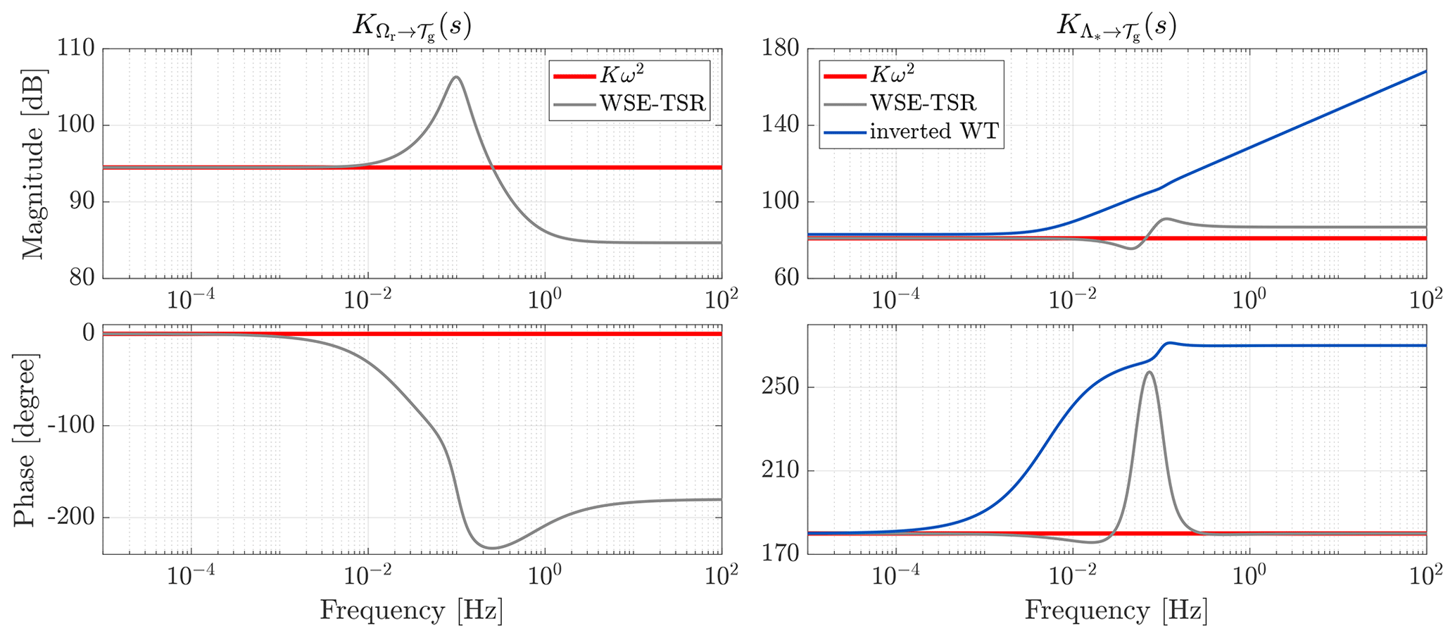
Figure 6 Bode plots of the controller transfer functions $K_{{\mathrm{\Omega }}_{\mathrm{r}}\to {\mathcal{T}}_{\mathrm{g}}}\left(s\right)$ and $K_{{\mathrm{\Lambda }}_{*}\to {\mathcal{T}}_{\mathrm{g}}}\left(s\right)$ for the Kω² controller (red line) and the WSE–TSR tracking controller (grey line) without optimal calibration. For the baseline, both transfer functions are frequency independent. For the combined scheme, in the low-frequency region, $K_{{\mathrm{\Omega }}_{\mathrm{r}}\to {\mathcal{T}}_{\mathrm{g}}}\left(s\right)$ and $K_{{\mathrm{\Lambda }}_{*}\to {\mathcal{T}}_{\mathrm{g}}}\left(s\right)$ have gains equal to the baseline. In particular, for the right-hand plot, the controller gains match the inverted model of the wind turbine (blue line), exhibiting a second-order lead–lag behaviour. By contrast, for higher frequencies, the response varies for both transfer functions for the combined scheme.

Equations (19) and (20) show that the controller transfer functions are merely frequency-independent static gains for the baseline controller. That is, the gain is constant over all frequencies. In contrast, the WSE–TSR tracking controller transfer functions possess dynamics (Eqs. 29 and 30). For this reason, it is assumed that for the low-frequency region, the (DC) gain of the latter controller equals the gain of the baseline controller, whereas, for higher frequencies, the frequency responses vary.

To examine the controller transfer functions, Eqs. (29) and (30) are symbolically evaluated as $s=\mathrm{j}\mathit{\omega }=\mathrm{0}$, with j being the imaginary unit number. By doing so, the steady-state responses of the WSE–TSR tracking controller transfer functions are computed, and after substitutions and simplifications, the following expressions are derived:

$$\begin{array}{}\text{(31)}& \begin{array}{rl}& K_{\left({\mathrm{\Omega }}_{\mathrm{r}}\to {\mathcal{T}}_{\mathrm{g}}\right),\mathrm{TSR}}(s=\mathrm{0})=-{\displaystyle \frac{\left(\stackrel{\mathrm{‾}}{V}\widehat{H}+{\stackrel{\mathrm{‾}}{\mathit{\omega }}}_{\mathrm{r}}\widehat{G}\right)}{{\stackrel{\mathrm{‾}}{\mathit{\omega }}}_{\mathrm{r}}E}}={\displaystyle \frac{\stackrel{\mathrm{‾}}{V}}{{\stackrel{\mathrm{‾}}{\mathit{\omega }}}_{\mathrm{r}}N}}\left({\displaystyle \frac{\partial {\widehat{T}}_{\mathrm{r}}}{\partial \widehat{V}}}\right)\\ & +{\displaystyle \frac{\mathrm{1}}{N}}\left({\displaystyle \frac{\partial {\widehat{T}}_{\mathrm{r}}}{\partial {\mathit{\omega }}_{\mathrm{r}}}}\right)={\displaystyle \frac{\mathit{\rho }{R}^{\mathrm{3}}{A}_{\mathrm{rot}}{C}_{\mathrm{p},*}\left({\mathit{\lambda }}_{*}\right)}{N{\mathit{\lambda }}_{*}^{\mathrm{3}}}}{\stackrel{\mathrm{‾}}{\mathit{\omega }}}_{\mathrm{r}},\end{array}\end{array}$$

$$\begin{array}{}\text{(32)}& \begin{array}{rl}& K_{\left({\mathrm{\Lambda }}_{*}\to {\mathcal{T}}_{\mathrm{g}}\right),\mathrm{TSR}}(s=\mathrm{0})={\displaystyle \frac{{\stackrel{\mathrm{‾}}{V}}^{\mathrm{2}}\widehat{H}}{R{\stackrel{\mathrm{‾}}{\mathit{\omega }}}_{\mathrm{r}}E}}=-{\displaystyle \frac{{\stackrel{\mathrm{‾}}{V}}^{\mathrm{2}}}{R{\stackrel{\mathrm{‾}}{\mathit{\omega }}}_{\mathrm{r}}N}}\left({\displaystyle \frac{\partial {\widehat{T}}_{\mathrm{r}}}{\partial \widehat{V}}}\right)\\ & ={\displaystyle \frac{\mathit{\rho }{R}^{\mathrm{3}}{A}_{\mathrm{rot}}}{\mathrm{2}N}}\left(-{\displaystyle \frac{\mathrm{3}}{{\mathit{\lambda }}_{*}^{\mathrm{4}}}}{C}_{\mathrm{p},*}\left({\mathit{\lambda }}_{*}\right)+{\displaystyle \frac{\mathrm{1}}{{\mathit{\lambda }}_{*}^{\mathrm{3}}}}{\displaystyle \frac{\partial C_{\mathrm{p},*}\left({\mathit{\lambda }}_{*}\right)}{\partial {\mathit{\lambda }}_{*}}}\right){\stackrel{\mathrm{‾}}{\mathit{\omega }}}_{\mathrm{r}}^{\mathrm{2}}.\end{array}\end{array}$$

It is immediately evident that $K_{\mathrm{TSR}}(s=\mathrm{0})=K_{\mathrm{K}}$ as defined earlier in Eqs. (19) and (20). This proves that the WSE–TSR tracking controller is equivalent to the Kω² controller in steady state. Thus, the two controllers will have the same static behaviour (Aström and Murray, 2010), operating at the same point of power extraction efficiency, $C_{\mathrm{p},*}\left({\mathit{\lambda }}_{*}\right)$.

Similarities and differences between the two controllers are further illustrated in Fig. 6 with Bode plots of the analysed controller transfer functions. The frequency responses are obtained using the NREL 5 MW reference turbine parameters (Jonkman et al., 2009) and a controller calibration that performs satisfactorily but is non-optimised. In the figure illustrating the Bode plot for $K_{{\mathrm{\Omega }}_{\mathrm{r}}\to {\mathcal{T}}_{\mathrm{g}}}\left(s\right)$ of both controllers, it can be observed that the two controllers show the same characteristics for the low-frequency region (between $\mathrm{1}\times {\mathrm{10}}^{-\mathrm{5}}$ and $\mathrm{1}\times {\mathrm{10}}^{-\mathrm{2}}$ Hz). However, for higher frequencies, the WSE–TSR tracking controller presents additional dynamics in the form of a resonance resulting from a complex left half-plane pole pair and a double right half-plane zero. The explanation for these additional dynamics is the controller attaining a higher open-loop unity crossover, resulting in an increased closed-loop control bandwidth. The right plot presents the frequency response for $K_{{\mathrm{\Lambda }}_{*}\to {\mathcal{T}}_{\mathrm{g}}}\left(s\right)$ and for the inverted transfer function of the wind turbine defined in Eq. (13). It is clear that both controllers exhibit a second-order lead–lag behaviour related to the model inversion required for the reference shaping action (Leith and Leithead, 1997).

4 Calibration of the WSE–TSR tracking control scheme

From the frequency-domain framework derived in the previous section, it is recognised that the WSE–TSR tracking controller presents a higher-dimensional design space than the baseline Kω². In particular, while the Kω² controller has only the torque gain K to calibrate, the combined scheme has a total of five variables: K_p,w, K_i,w, K_p,c, K_i,c and λ_*. This tight integration between a disturbance estimator and a tracking controller makes the mutual calibration of the design variables in the WSE–TSR tracking controller a complex and non-trivial task. Therefore, this section addresses the calibration of the controller by formulating a multi-objective optimisation problem. The approach to solving this multi-objective problem is by reconstructing (an approximation of) the true Pareto front, composed of a set of Pareto optimal solutions. To this end, first, the multi-objective optimisation problem is formalised in Sect. 4.1 and implemented in Sect. 4.2. An exploratory and guided search over the controller calibration variables examines the performance space formed by all objectives. The outcomes of this search are presented in Sect. 4.3 to construct approximations of the true Pareto front, which are related to the controller calibrations.

4.1 Multi-objective optimisation

A multi-objective optimisation problem is considered over a set of continuous input variables 𝒳⊂ℝ^d called the design space (Lukovic et al., 2020). The optimisation goal is to minimise the vector of the objective functions defined as f(x)=(f₁(x), ⋯, f_m(x))) with m≥2, x∈𝒳 being the vector of input variables and f(𝒳)⊂ℝ^m the m-dimensional image representing the performance space.

The conflicting nature of the objective functions does not always allow for the finding of a single best solution to the minimisation problem but rather a set of optimal solutions, referred to as the Pareto set 𝒫_s⊆𝒳 in the design space and the Pareto front ${\mathcal{P}}_{\mathrm{f}}=\mathit{f}\left({\mathcal{P}}_{\mathrm{s}}\right)\subset {\mathbb{R}}^m$ in the performance space (Lukovic et al., 2020). In the following, the Pareto front is approximated by considering the Pareto optimal to be the point ${\mathit{x}}_{*}\in {\mathcal{P}}_{\mathrm{s}}$, for which there is no other point x∈𝒳 such that $f_j\left({\mathit{x}}_{*}\right)\ge f_j\left(\mathit{x}\right)$ for all j values and $f_j\left({\mathit{x}}_{*}\right)>f_j\left(\mathit{x}\right)$ for at least one j, with j={1, ⋯, m} (Miettinen, 1999).

4.2 Implementation of the optimisation framework

The methodology for calibrating the design variables of the WSE–TSR tracking control scheme is addressed as the multi-objective optimisation problem previously described. A two-dimensional vector of the objective functions is considered. The first objective is the variance of the torque control signal, representing the responsiveness of the controller (i.e. a measure of its response speed). This objective can also act as a measure of loads on the structural components of the turbine. The second objective is the mean generated power of the wind turbine. These two objectives are conflicting as a more responsive controller is expected to result in higher power production levels with increased loads and a fast response time and vice-versa for milder controller calibration. Thereby, the objective function vector is given by

$$\begin{array}{}\text{(33)}& \mathit{f}\left({\mathbf{\Gamma }}_{\mathrm{d}}\right)=\left[f_{\mathrm{1}}\left({\mathbf{\Gamma }}_{\mathrm{d}}\right),f_{\mathrm{2}}\left({\mathbf{\Gamma }}_{\mathrm{d}}\right)\right],\end{array}$$

with the torque variance being defined as

$$f_{\mathrm{1}}\left({\mathbf{\Gamma }}_{\mathrm{d}}\right)={\displaystyle \frac{\sum _{i=\mathrm{1}}^n{\left(T_{\mathrm{g},\mathrm{i}}\left({\mathbf{\Gamma }}_{\mathrm{d}}\right)-T_{\mathrm{g},\mathrm{mean}}\left({\mathbf{\Gamma }}_{\mathrm{d}}\right)\right)}^{\mathrm{2}}}{n}}$$

and the mean power as

$$f_{\mathrm{2}}\left({\mathbf{\Gamma }}_{\mathrm{d}}\right)=-{\displaystyle \frac{\sum _{i=\mathrm{1}}^n{P}_{\mathrm{g},\mathrm{i}}\left({\mathbf{\Gamma }}_{\mathrm{d}}\right)}{n}}.$$

In the above equations, n is the number of data points; T_g,mean is the mean value of the generator torque; and T_g,i and P_g,i represent each value of generator torque and power in the dataset (Brandetti, 2023), respectively. As shown, the resulting signals T_g and P_g are a function of ${\mathbf{\Gamma }}_{\mathrm{d}}\in {\mathcal{X}}_{\mathrm{d}}\subset {\mathbb{R}}^{\mathrm{d}}$, which is the d-dimensional vector of input variables. In this study, the dimensionality of the input vectors is investigated to assess the performance of the controller for different levels of complexity as

$$\begin{array}{ll}{\displaystyle }& {\displaystyle }{\mathbf{\Gamma }}_{\mathrm{5}}=\left[K_{\mathrm{p},\mathrm{c}},K_{\mathrm{i},\mathrm{c}},K_{\mathrm{p},\mathrm{w}},K_{\mathrm{i},\mathrm{w}},{\mathit{\lambda }}_{*}\right]\in {\mathcal{X}}_{\mathrm{5}},\\ {\displaystyle }& {\displaystyle }{\mathbf{\Gamma }}_{\mathrm{4}}=\left[K_{\mathrm{p},\mathrm{c}},K_{\mathrm{i},\mathrm{c}},K_{\mathrm{p},\mathrm{w}},{\mathit{\lambda }}_{*}\right]\in {\mathcal{X}}_{\mathrm{4}},\\ {\displaystyle }& {\displaystyle }{\mathbf{\Gamma }}_{\mathrm{3}}=\left[K_{\mathrm{i},\mathrm{c}},K_{\mathrm{p},\mathrm{w}},{\mathit{\lambda }}_{*}\right]\in {\mathcal{X}}_{\mathrm{3}},\\ {\displaystyle }& {\displaystyle }{\mathbf{\Gamma }}_{\mathrm{2}}=\left[K_{\mathrm{i},\mathrm{c}},K_{\mathrm{p},\mathrm{w}}\right]\in {\mathcal{X}}_{\mathrm{2}},\\ {\displaystyle }& {\displaystyle }{\mathbf{\Gamma }}_{\mathrm{1}}=\left[{\mathit{\lambda }}_{*}\right]\in {\mathcal{X}}_{\mathrm{1}},\end{array}$$

where the subscript (⋅)_d represents the dimension of each design space and is used in the remainder of this paper to differentiate between the input vectors. Note that d=5 refers to the original formulation of the WSE–TSR tracking controller, for which the integral term in the estimator (K_i,w) was introduced recently in the work of Liu et al. (2022). The integral term ensures that the internal estimated rotor speed state is consistent with the actual rotor speed measurement. Furthermore, combining a proportional and integral term (K_p,w and K_i,w) results in a faster estimation convergence by rapidly reducing the estimation error. The input vectors Γ_d⊂Γ₅ for d={2, 3, 4}, while, Γ₁ represents the one-dimensional design space of the Kω² controller, in which the variation in λ_* leads to variation in the gain K according to Eq. (5). Furthermore, as can be recognised from the defined input vectors Γ_d, the estimator and controller are consistently and intricately calibrated in unison throughout the entire work.

Aero-servo-elastic simulations are performed with NREL's mid-fidelity wind turbine simulation software OpenFAST (NREL, 2021) to compute the objective function vector f(Γ_d). The NREL 5 MW reference wind turbine (Jonkman et al., 2009) is subject to a realistic turbulent wind profile with a mean wind speed of $\stackrel{\mathrm{‾}}{V}=\mathrm{9}$ m s⁻¹ at hub height and a turbulence intensity of TI = 15 %. Under these operational conditions, the multi-objective optimisation is performed. For each simulation, the input vector is constrained for a guided search to find a set of optimal solutions ${\mathcal{P}}_{\mathrm{s}}^{\mathrm{d}}\subset {\mathbb{R}}^{\mathrm{d}}$ to approximate the Pareto front ${\mathcal{P}}_{\mathrm{f}}^{\mathrm{d}}=\mathit{f}\left({\mathcal{P}}_{\mathrm{s}}^{\mathrm{d}}\right)$. Simulations are run in parallel by randomly varying the input vector inside the constrained design space. Each simulation has a length of 3600 s, of which the first 100 s is discarded to exclude the transient start-up effects from the results. The acquired time series is used to calculate the considered objectives f₁(Γ_d) and f₂(Γ_d).

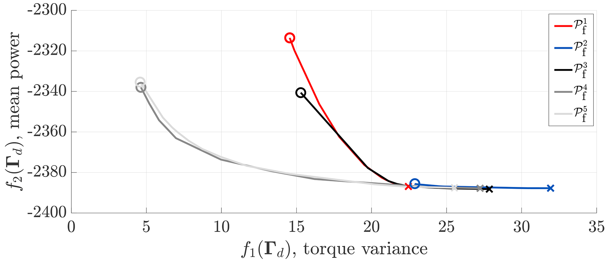
Figure 7 Pareto fronts obtained for the WSE–TSR tracking control scheme for different sets of estimator-controller design variables: Γ₁, Γ₂, Γ₃, Γ₄ and Γ₅. Simulations are performed with NREL's mid-fidelity wind turbine simulation software OpenFAST (NREL, 2021) under realistic turbulent wind conditions. The objective functions f₁(Γ_d), i.e. torque fluctuation minimisation, and f₂(Γ_d), i.e. power maximisation, define the performance space for the controller. The optimal solutions for f₁(Γ_d) and f₂(Γ_d) are indicated using circles (∘) and crosses (×), respectively. Compared to the baseline controller represented by the Pareto front ${\mathcal{P}}_{\mathrm{f}}^{\mathrm{1}}$, the WSE–TSR tracking controller does not attain an enhancement in power maximisation but allows the minimisation of torque fluctuations with a small penalty in power extraction.

4.3 Optimisation results

This section presents the results obtained with the described optimisation framework. The performance space is explored using the guided search for the five sets of calibration input variables. Subsequently, the results are used to approximate the corresponding Pareto fronts. Finally, the influence of the gains is assessed by analysing the different regions of the constrained design space.

4.3.1 Exploratory search and Pareto front

Before constructing the Pareto front, the performance space is explored by means of a guided search of the input variables Γ_d. With an increasing dimension d of the design space, more data are collected to capture the performance space of interest effectively. The conventional Kω² controller is used as a baseline comparison case.

With the exploration data at hand, the Pareto front is approximated by minimising a weighted linear combination of f₁(Γ_d) and f₂(Γ_d) on the complete dataset and for a range of weights. As shown in Fig. 7, Pareto fronts are approximated for different dimensionalities of the input vector Γ_d to compare the baseline to the performance of the WSE–TSR tracking controller. The optimal solutions based on each objective function f₁(Γ_d) and f₂(Γ_d) are indicated using circles (∘) and crosses (×), respectively.

From the figure, it is immediately apparent that the fronts of the higher-dimensional controllers d={4, 5} cover the widest area of the performance space; the remaining fronts are subsets of the original WSE–TSR tracking control scheme. Since the Pareto fronts for d={4, 5} overlap, it is concluded that adding an integral term to the estimator (i.e. K_i,w) leads to no (or marginal) benefits with respect to the performance of the WSE–TSR tracking scheme. It follows that only by adding a proportional control gain (i.e. K_p,c) it leads to more flexibility in reaching desired (Pareto) optimal solutions minimising torque fluctuations and corresponding (structural) loads, with a minimal impact on the power extraction performance. This shows the benefits of the more flexible structure of the WSE–TSR tracking scheme.

Another observation is that the baseline controller already attains a Pareto optimal solution minimising f₂(Γ_d), i.e. maximising power production. It is clear that increasing the controller bandwidth and allowing for higher torque fluctuations f₁(Γ_d) do not result in the enhancement of energy capture f₂(Γ_d) compared to the baseline control strategy. A plausible explanation is that the higher inertia of large-scale wind turbines inherently provides resilience against deviations from the optimal operating point. Therefore, increasing the controller bandwidth resulting in tighter tracking to the desired tip-speed ratio reference might not directly result in additional benefits in terms of energy capture.

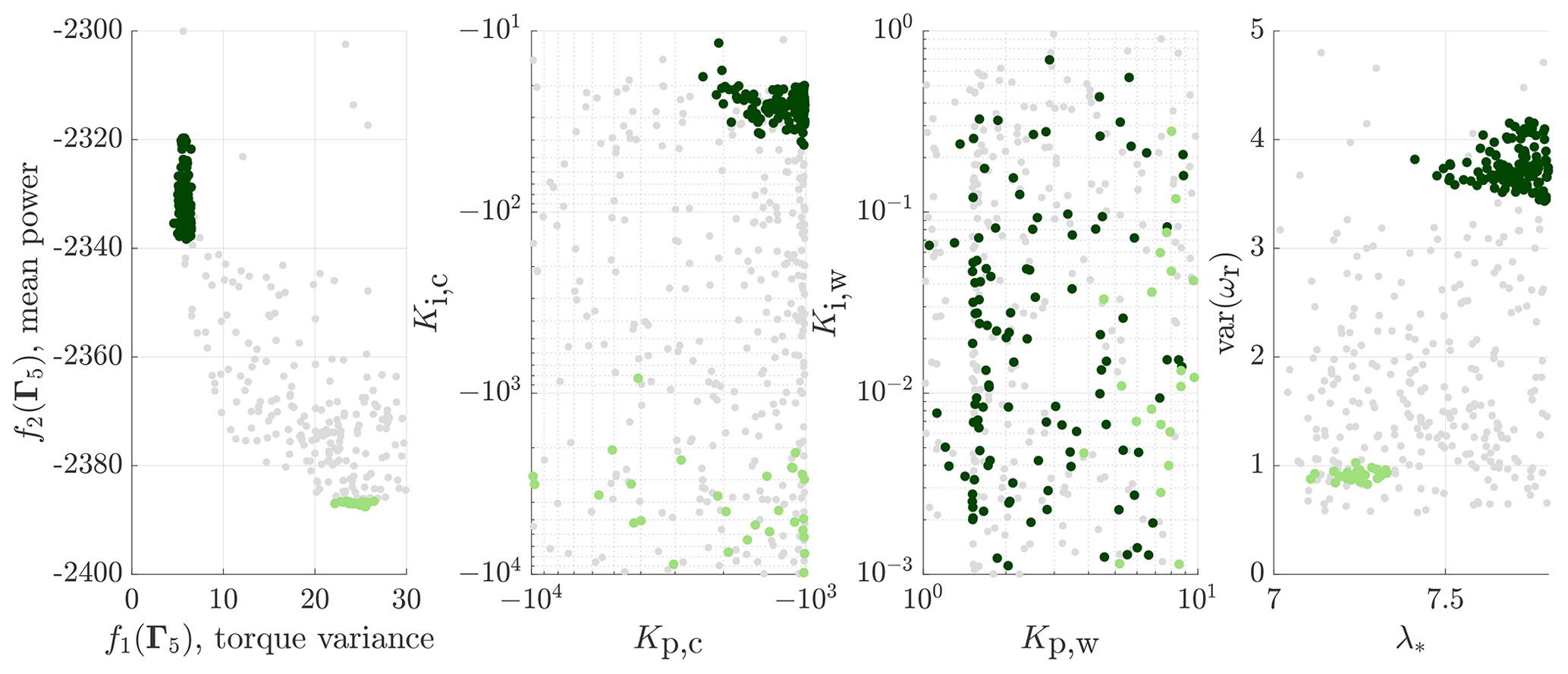
Figure 8 Results for the WSE–TSR tracking control scheme obtained with an exploratory search of its design variables (i.e. Γ₅). Different shades of green are used to highlight two areas of interest: the lowest values of f₁(Γ₅) (torque fluctuation minimisation) and f₂(Γ₅) (power maximisation). The two objectives and the rotor speed variance (var(ω_r)) are plotted together with the controller gains (K_p,c and K_i,c), the estimator gains (K_p,w and K_i,w) and the reference tip-speed ratio (λ_*) to show how these calibration variables influence the scheme's performance. Clearly, neither K_i,w nor K_p,c correlates to the performance of the WSE–TSR tracking controller. While λ_* and K_p,w follow an increasing trend proportional to the increase in torque variance, K_i,c exhibits the opposite behaviour.

4.3.2 Influence of the controller calibration variables

This section qualitatively assesses the influence of the gains on and correlation of the gains to the performance of the WSE–TSR tracking controller. The analysis is presented in Fig. 8, where two areas of interest are selected: the lowest value of f₂(Γ₅) (power maximisation) and f₁(Γ₅) (torque fluctuation minimisation). The analysis only draws conclusions relating the calibration of the scheme to the considered objectives; a more formal frequency- and time-domain analysis is described in the next section. Furthermore, only the five-dimensional input vector Γ₅ will be evaluated from this point onwards, as the current study focuses on providing calibration guidelines for the complete WSE–TSR tracking control scheme rather than for its subsets.

For the power maximisation case, λ_* should be taken between 7.1 and 7.3, which corresponds to the region of maximum power extraction for the NREL 5 MW (Fig. 1). For the torque minimisation case, λ_* should be chosen as higher than the power-coefficient-maximising value, resulting in a power reduction and rotational speed variance increase. Furthermore, as observed from both cases, K_p,w follows an increasing trend proportional to the increase in torque variance, while K_i,w does not show a clear correlation to the controller performance.

Considering the controller gains, it is clear that the controller relies heavily on integral action to track the desired tip-speed ratio reference and therefore achieve power maximisation. The gain for the proportional action K_p,c lies in the same area for the two regions of interest without directly influencing the performance.

5 Analysis of optimally calibrated WSE–TSR tracking controllers

Pareto fronts are approximated in the previous section, representing a set of optimal solutions among the conflicting objectives. An analysis is presented by directly relating the objectives to the input vectors of various dimensionalities. This section compares the characteristics of full-dimensional and optimally calibrated WSE–TSR tracking controllers to the baseline Kω² strategy.

The initial step in this comparison involves a qualitative assessment of the impact of optimal calibrations on system parameters. Subsequently, to provide specific guidance for the optimal calibration of the controller, a sensitivity analysis examines the effect of each calibration variable on corresponding objectives and turbine loads. To conclude the study, the frequency-domain framework outlined in Sect. 3 is applied alongside mid-fidelity time-domain simulations to replicate realistic turbulent wind conditions.

5.1 Case study definition

The case studies analysed in this section are presented in Fig. 9. The figure shows the approximated Pareto fronts ${\mathcal{P}}_{\mathrm{f}}^{\mathrm{5}}$ and ${\mathcal{P}}_{\mathrm{f}}^{\mathrm{1}}$, representing the WSE–TSR tracking and the baseline controllers, respectively. Along the ${\mathcal{P}}_{\mathrm{f}}^{\mathrm{5}}$ front, five distinct optimal solutions are chosen, and the corresponding calibrations Γ₅ are considered for analysis in the following subsections. The selection considers the evaluation of different trade-off levels between the considered objectives from the point of maximum power extraction (A) to the point of minimum torque variance (E). Point B is the closest to the maximum power extraction of the Kω² controller and is selected to show similarities between these two schemes.

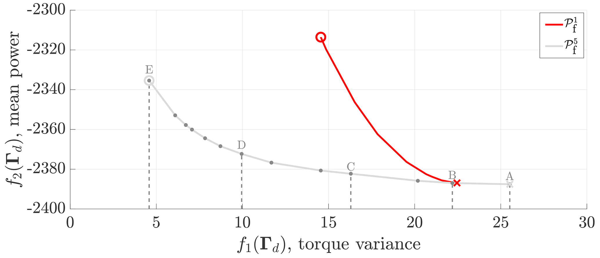
Figure 9 Pareto fronts ${\mathcal{P}}_{\mathrm{f}}^{\mathrm{1}}$ and ${\mathcal{P}}_{\mathrm{f}}^{\mathrm{5}}$ obtained for the baseline and WSE–TSR tracking control schemes and related to the Γ₁ and Γ₅ design variables. Simulations are performed with NREL's mid-fidelity wind turbine simulation software OpenFAST (NREL, 2021) under realistic turbulent wind conditions. The case studies for the WSE–TSR tracking controller are marked on the ${\mathcal{P}}_{\mathrm{f}}^{\mathrm{5}}$ front with letters ranging from A to E, corresponding to maximum power extraction and minimum generator torque fluctuations, respectively. Point B is the closest to the optimal baseline controller calibration in terms of power extraction.

5.2 Qualitative assessments of optimal controller solutions

This section provides an overview of how optimal calibration points, as defined in Sect. 5.1, impact the system parameters, especially load components. The assessment is performed qualitatively as a first step to offering calibration guidelines for the WSE–TSR tracking controller. The analysis outcomes are summarised in Table 2, where symbols ◦, $++$, +, − and $--$ denote no influence, really positive influence, positive influence, negative influence and really negative influence on the performance metrics.

Table 2 Qualitative assessments of the Kω² controller and the different WSE–TSR tracking controllers ranging from the maximum power extraction (A) to the minimum generator torque fluctuation (E) optimal calibrations. The following system quantities are used for the analysis: f₁(Γ_d) (torque fluctuation minimisation), f₂(Γ_d) (power maximisation), rotor speed variance, the fore–aft tower moment (FATM), the side-to-side tower moment (SSTM), the flapwise bending moment for blade 1 (FlapBM) and the edgewise bending moment for blade 1 (EdgeBM). For each tower and blade load, two values are presented that correspond to the mean and variance, respectively. No influence, really positive influence, positive influence, negative influence and really negative influence of the considered controllers are indicated with ◦, $++$, +, − and $--$, respectively.

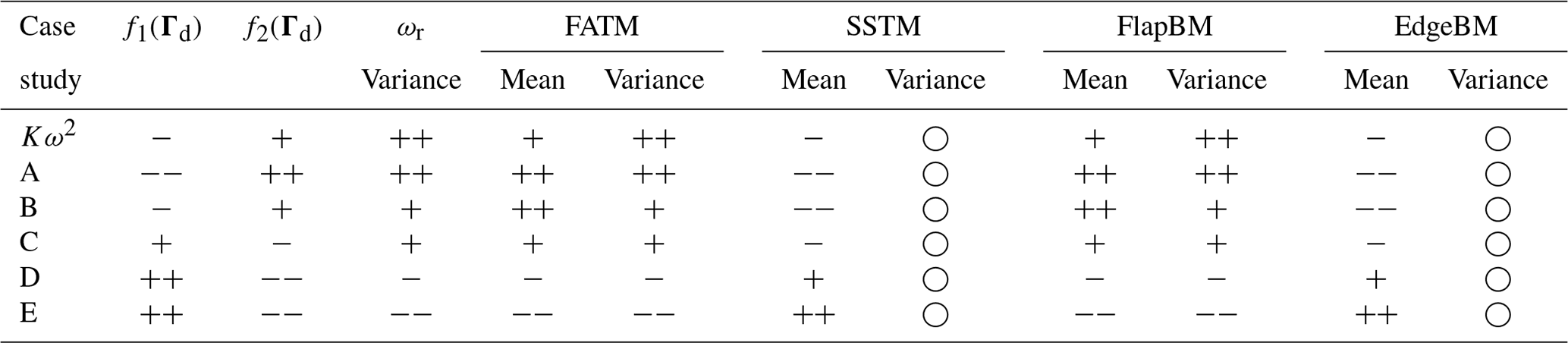
As points A and E have a positive effect on maximising power extraction, f₂(Γ₅), and on minimising generator torque fluctuations, f₁(Γ₅), respectively, it is confirmed that they represent the extremes of the Pareto front ${\mathcal{P}}_{\mathrm{f}}^{\mathrm{5}}$. Point B emerges as the calibration point closest to the optimal Kω² controller calibration in terms of power extraction. As the cases progress towards E, the primary aim of the controller is to minimise the generator torque variance, leading to a reduction in bandwidth. Consequently, these controllers positively affect the mean side-to-side tower moment (SSTM) and the edgewise blade 1 moment (EdgeBM). However, this improvement negatively influences the rotor speed variance as well as the mean and variance of both the fore–aft tower moment (FATM) and the flapwise blade 1 moment (FlapBM). Overall, the optimal controller calibrations under consideration do not affect the variance of the side-to-side tower moment and the edgewise blade 1 moment. A coupling is evident between the fore–aft and flapwise moments and between the side-to-side and edgewise moments. This intricate interplay proves the complexity of calibrating the WSE–TSR tracking control scheme, as several system parameters are intertwined, and confirms the need for a multi-objective optimisation framework and a frequency-domain analysis to link controller insight with turbine performance metrics.

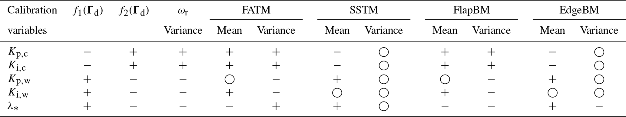
Table 3 Sensitivity analysis of the optimal controller calibration C for the WSE–TSR tracking controller. For each row, the corresponding calibration variable is varied, while the others are kept fixed to the optimal value. The following system quantities are used for the analysis: f₁(Γ_d) (torque fluctuation minimisation), f₂(Γ_d) (power maximisation), rotor speed variance, the fore–aft tower moment (FATM), the side-to-side tower moment (SSTM), the flapwise bending moment for blade 1 (FlapBM) and the edgewise bending moment for blade 1 (EdgeBM). For each tower and blade load, two values are presented that correspond to the mean and variance, respectively. No influence, positive influence and negative influence of the considered calibration variable are indicated with ◦, + and −, respectively.

5.3 Sensitivity analysis of optimal calibration variables

This section aims to comprehensively evaluate the effect of the optimal calibration variables on various system parameters. An optimally calibrated WSE–TSR tracking controller is selected from the case studies outlined in Sect. 5.1 for this sensitivity analysis. Specifically, controller C is chosen to represent a trade-off between minimising generator torque fluctuations and maximising power production. For this controller, the five calibration variables – K_p,c, K_i,c, K_p,w, K_i,w and λ_* – are assessed in terms of their positive or negative influence on the turbine performance metrics. The gains are varied individually, while keeping the others fixed to their optimal value. The analysis results are summarised in Table 3, where each row corresponds to the effect of increasing the absolute value of each calibration variable.

As observed, increasing K_p,c and K_i,c, relative to their optimal value, positively affects f₂(Γ_d), the rotor speed variance and the reduction of the mean and variance of the fore–aft tower moment and flapwise bending moment for blade 1. This benefit, however, negatively impacts f₁(Γ_d) and the mean of the side-to-side tower moment and edgewise bending moment for blade 1. No apparent influence is noted on the variance of the latter variables. These findings further confirm the coupling between the fore–aft and flapwise moments and between the side-to-side and edgewise moments. Conversely, an opposite trend for f₁(Γ_d), f₂(Γ_d) and the rotor speed variance is observed when increasing K_p,w, K_i,w and λ_* beyond their optimal values. These observations confirm that optimal tuning of the calibration variables for the WSE–TSR tracking controller is needed to achieve a trade-off between power maximisation and torque minimisation.

5.4 Frequency-domain results

This section compares the frequency-domain characteristics for the defined cases using the linear analysis framework described in Sect. 3. First, the frequency responses for the controller transfer functions $K_{{\mathrm{\Omega }}_{\mathrm{r}}\to {\mathcal{T}}_{\mathrm{g}}}\left(s\right)$ and $K_{{\mathrm{\Lambda }}_{*}\to {\mathcal{T}}_{\mathrm{g}}}\left(s\right)$ are discussed, followed by the closed-loop transfer functions $T_{{\mathrm{\Lambda }}_{*}\to \mathrm{\Lambda }}\left(s\right)$ and T_𝒱→Λ(s).

5.4.1 Controller transfer functions

The analysis strategy defined in Sect. 3.2 is employed to evaluate the characteristics of the controllers. The frequency responses of the transfer functions $K_{{\mathrm{\Omega }}_{\mathrm{r}}\to {\mathcal{T}}_{\mathrm{g}}}\left(s\right)$ and $K_{{\mathrm{\Lambda }}_{*}\to {\mathcal{T}}_{\mathrm{g}}}\left(s\right)$ for the defined cases are presented in Fig. 10. The results for the Kω² controller are included as a baseline, being frequency independent with a constant gain over all frequencies.

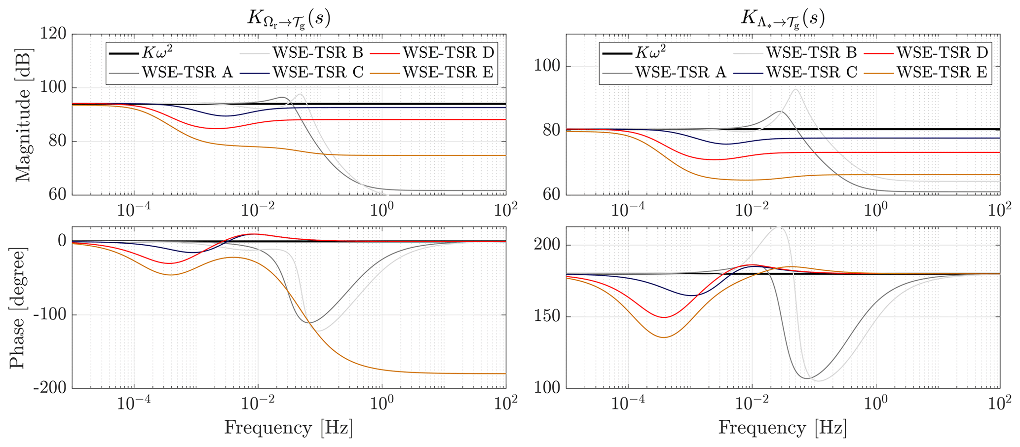
Figure 10 Bode plots of the controller transfer functions $K_{{\mathrm{\Omega }}_{\mathrm{r}}\to {\mathcal{T}}_{\mathrm{g}}}\left(s\right)$ and $K_{{\mathrm{\Lambda }}_{*}\to {\mathcal{T}}_{\mathrm{g}}}\left(s\right)$ for the baseline Kω² and the WSE–TSR tracking controller cases. For the baseline, $K_{({\mathrm{\Omega }}_{\mathrm{r}}\to {\mathcal{T}}_{\mathrm{g}}),K}$ and $K_{({\mathrm{\Lambda }}_{*}\to {\mathcal{T}}_{\mathrm{g}}),K}$ show a constant gain over all frequencies, while for the WSE–TSR tracking controllers, $K_{({\mathrm{\Omega }}_{\mathrm{r}}\to {\mathcal{T}}_{\mathrm{g}}),TSR}\left(s\right)$ and $K_{({\mathrm{\Lambda }}_{*}\to {\mathcal{T}}_{\mathrm{g}}),TSR}\left(s\right)$ exhibit additional dynamics with an increasing cut-off frequency for increasing cases towards B. In particular, cases A and B present resonance peaks in their response to further improve the controller cut-off frequency.

For case E, the steady-state gain deviates from the baseline gain because the reference tip-speed ratio is calibrated at a higher and non-optimal set point of ${\mathit{\lambda }}_{*}^{\mathrm{E}}=\mathrm{7.71}$. Furthermore, for the same case, it is seen that the controller cut-off frequencies are at the lowest frequency compared to the other cases, resulting in reduced torque variance responses. For increasing points towards case A, the controller cut-off frequency for both reference shaping and feedback-related transfer functions increases to higher frequencies, except for B. As shown in Fig. 9, case B shows the closest resemblance with respect to performance attained with the optimal baseline controller. A possible explanation is that the controller adheres to the Kω² trajectory for the most extended frequency range. A notable observation is the resonance peaks for cases A and B, which enable a higher cut-off frequency of the loop gain, resulting in an increased closed-loop bandwidth to track the desired tip-speed ratio. In this context, it is essential to consider that while a slight increase in power performance is observed for case A, it is accompanied by elevated torque fluctuations. Therefore, having a controller with a bandwidth exceeding that of case A would not be advantageous, as it would likely be more aggressive, potentially leading to system instability and yielding no power gain at the expense of increased torque fluctuations. A further observation from the phase plots is the opposite sign of the controller transfer functions, which is understandable from a physical perspective. The generator torque increases for higher rotational speeds ($K_{{\mathrm{\Omega }}_{\mathrm{r}}\to {\mathcal{T}}_{\mathrm{g}}}\left(s\right)$), whereas an inverse proportional relation exists between the desired tip-speed ratio and generator torque ($K_{{\mathrm{\Lambda }}_{*}\to {\mathcal{T}}_{\mathrm{g}}}\left(s\right)$).

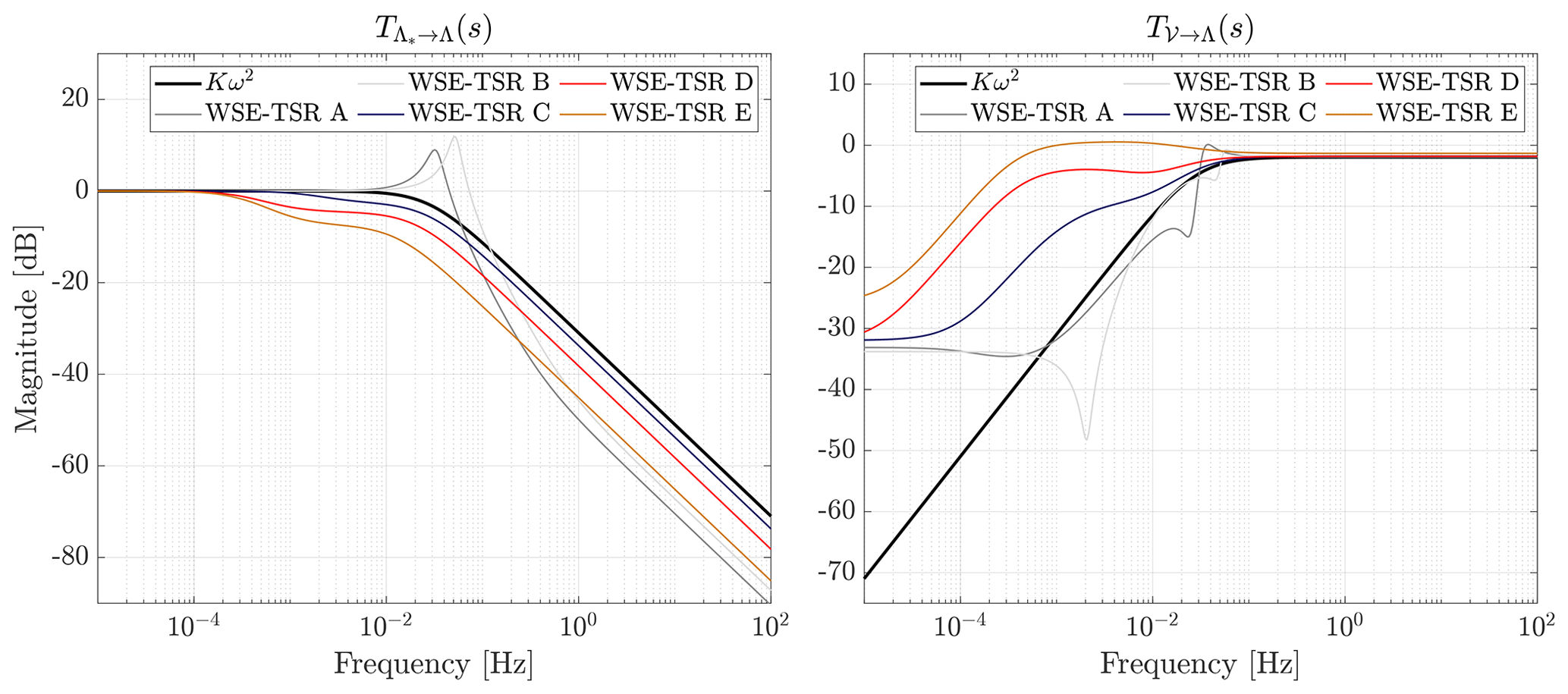
Figure 11 Bode plots of the closed-loop transfer functions $T_{{\mathrm{\Lambda }}_{*}\to \mathrm{\Lambda }}\left(s\right)$ and T_𝒱→Λ(s) for the baseline Kω² and the WSE–TSR tracking controller cases. Regarding $T_{{\mathrm{\Lambda }}_{*}\to \mathrm{\Lambda }}\left(s\right)$, an increase in controller bandwidth with respect to the baseline can be observed when the calibration selected aims to maximise the power performance (i.e. A and B). On the other hand, for T_𝒱→Λ(s), this improvement is translated into a high-frequency sensitivity deterioration.

5.4.2 Closed-loop transfer functions

This section presents an analysis of the closed-loop controller characteristics. For the different cases, Fig. 11 illustrates the frequency responses of the transfer functions $T_{{\mathrm{\Lambda }}_{*}\to \mathrm{\Lambda }}\left(s\right)$ and T_𝒱→Λ(s), representing the closed-loop system performance in terms of reference tracking (complementary sensitivity) and disturbance rejection (sensitivity), respectively. The results for these transfer functions confirm the observations in the open-loop analysis: increasing points toward point A exhibit an increased bandwidth and reference-tracking performance. Furthermore, only points A and B show a resonance peak resulting in a higher closed-loop cut-off frequency. For the transfer function T_𝒱→Λ(s), it is concluded that cases C, D and E are subpar in disturbance rejection performance compared to the baseline case. In addition, the effect of the Bode sensitivity integral is represented by the two remaining cases. That is, cases A and B show increased disturbance rejection performance for frequencies below the controller bandwidth, whereas, after this value, the characteristics worsen with respect to the baseline controller.

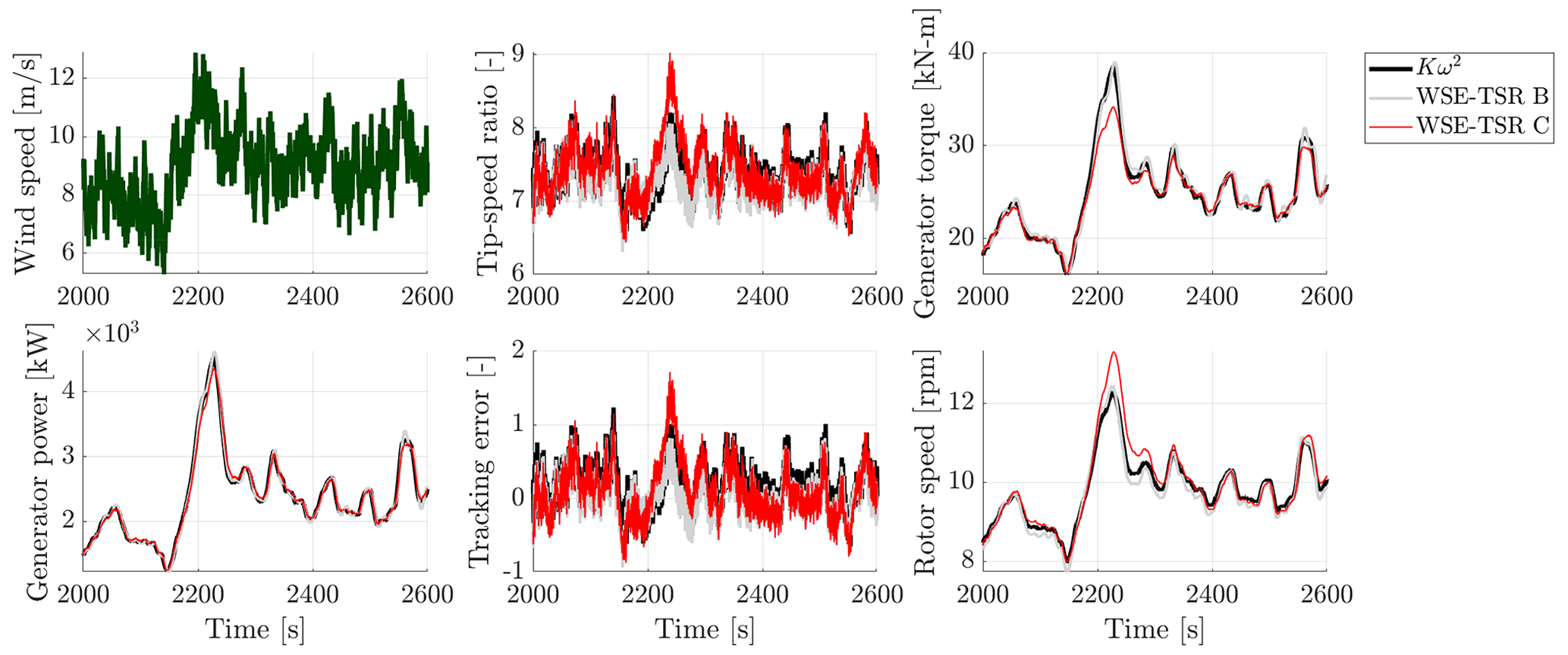
Figure 12 Simulation results for the Kω² and WSE–TSR tracking controllers subject to a realistic turbulent wind speed with a mean of 9 m s⁻¹ and a turbulence intensity of 15 %. Only results for cases B and C are presented. As expected from the location on the corresponding Pareto front ${\mathcal{P}}_{\mathrm{f}}^{\mathrm{5}}$, case B shows a similar performance to the baseline control strategy. On the other hand, case C represents a trade-off between the two objectives, minimising torque fluctuations with a minor impact on power production.

5.5 Time-domain results

To further support the observations from the frequency-domain analysis, this section presents realistic time-domain simulation results. For the sake of clarity, only two input vectors Γ₅ corresponding to cases B and C are chosen. This selection aims to illustrate the characteristics of the WSE–TSR tracking controller for the optimal solution f₂(Γ_d) and the trade-off between f₁(Γ_d) and f₂(Γ_d) compared to the baseline controller.

The mid-fidelity simulation is performed with OpenFAST using the NREL 5 MW reference turbine for a realistic turbulent wind profile, with a mean wind speed of $\stackrel{\mathrm{‾}}{V}=\mathrm{9}$ m s⁻¹ at hub height, a turbulence intensity of TI = 15 % and a total simulation time of 3600 s. Figure 12 shows the wind speed and the simulation results for the tip-speed ratio, tip-speed ratio tracking error, generator torque, rotor speed and generator power. A smaller portion of the simulation is presented to emphasise the features in the time-domain results.

The WSE–TSR tracking controller, calibrated for case B, demonstrates performance comparable to the baseline controller without exhibiting superior power production. These observations align with the trends of the Pareto front illustrated in Fig. 9. Simulation results obtained for case C show reduced torque fluctuations at the expense of increased oscillations in the rotor speed. This particular calibration results in a slower response of the WSE–TSR tracking controller, rendering the wind turbine more susceptible to variations in wind speed and, consequently, leading to higher fluctuations in rotor speed.

Upon closer examination, a notable instance occurs around 2200 s, wherein a change in wind speed from 8 to 12 m s⁻¹ prompts a corresponding change in rotor speed from 8 to 13 rpm and an alteration in the tip-speed ratio from 7 to 9. During this transition period, the tip-speed ratio deviates from the reference λ_*, slightly increasing the tip-speed ratio tracking error (i.e. $\mathit{\lambda }-{\mathit{\lambda }}_{*}$). However, a minimal impact can be observed in power extraction from the wind, confirming that tuning C provides a good trade-off between power maximisation and load minimisation for the considered turbine.

6 Conclusions

This study presents a detailed analysis of the conventional Kω² and the more advanced WSE–TSR tracking scheme, being a combined estimator-based tracking controller. A linear frequency-domain framework is derived to evaluate the characteristics of both control schemes. A unified analysis strategy is proposed for a fair comparison of the controllers.

To explore the performance potential of both control schemes and, more specifically, to discover whether the advanced controller provides benefits over the conventional one, a multi-objective optimisation problem is defined. The conflicting objectives are power maximisation and control signal variance minimisation. The approach to solving this optimisation problem is to explore the performance space using a constrained guided search for different dimensionalities of the design space. In other words, the controller calibration parameters have been categorised in input vectors of different dimensions, each subject to the multi-objective optimisation problem. The resulting Pareto front approximations represent the optimal solutions and controller calibrations, providing a trade-off between the defined objectives and dictating the selection of the specific controller bandwidth. A set of Pareto optimal solutions is evaluated in the frequency and time domains to provide more comprehensive insights into the balance between performance metrics and control dynamics, enabling users of the WSE–TSR tracking control scheme to make informed decisions on its optimal calibration.

Numerical simulations on the NREL 5 MW reference turbine show that an optimally calibrated WSE–TSR tracking control scheme can increase the controller bandwidth, resulting in larger torque fluctuations. However, as opposed to claims about improved power capture in the literature, no power gains are attainable for present-day relevant turbine sizes compared to baseline control. On the other hand, the proposed calibration framework makes it possible to find a set of design variables for the WSE–TSR tracking control scheme that reduces torque fluctuations with a minor impact on the captured power.

Overall, the WSE–TSR tracking controller exhibits a more flexible control structure compared to the baseline Kω² controller, providing a trade-off between power and load objectives that can facilitate the operation of large-scale modern wind turbines. Future work will focus on performing a similar analysis on smaller-scale wind turbines to confirm these benefits even for other commercial turbines.

Appendix A: Similarity to state feedback controller design

This section proves that by following the state feedback control design theory, it is possible to end up with equal results for the analysis strategy proposed for the Kω² controller, as illustrated in Fig. A1. First, the wind turbine to be controlled is assumed to be described by a linear state model with a single input T_g,K, a single output ω_r and a single state ω_r (Aström and Murray, 2010):

$$\begin{array}{}\text{(A1)}& {\dot{\mathit{\omega }}}_{\mathrm{r}}=A{\mathit{\omega }}_{\mathrm{r}}+B{T}_{\mathrm{g},\mathrm{K}},{\mathit{\omega }}_{\mathrm{r}}=C{\mathit{\omega }}_{\mathrm{r}}+D{T}_{\mathrm{g},\mathrm{K}},\end{array}$$

where A=G(V), B=E, C=1 and D=0.

By applying Assumption 1.1, the model general time-invariant control law is a function of the state and the reference input:

$$T_{\mathrm{g},\mathrm{K}}=\mathit{\alpha }\left({\mathit{\omega }}_{\mathrm{r}},{\mathit{\lambda }}_{*}\right).$$

If the feedback is restricted to be linear, it can be written as

$$\begin{array}{}\text{(A2)}& T_{\mathrm{g},\mathrm{K}}=-K_{\mathrm{f}}{\mathit{\omega }}_{\mathrm{r}}+k_{\mathrm{r}}{\mathit{\lambda }}_{*},\end{array}$$

in which K_f is the feedback gain, k_r is the reference shaping gain and λ_* is assumed to be a constant reference signal. This representation illustrates the baseline controller with elements K_f and k_r in a similar form as the analysis strategy presented in Eq. (14). Therefore, to prove that the Kω² controller is equivalent to a state feedback controller with reference shaping, Eq. (14) should match Eq. (A2), as

$$\begin{array}{}\text{(A3)}& K_{\mathrm{1},\mathrm{K}}=-K_{\mathrm{f}},\text{and}{K}_{\mathrm{2},\mathrm{K}}=k_{\mathrm{r}}.\end{array}$$

Assuming that this equality is valid, it results in

$$\begin{array}{}\text{(A4)}& \begin{array}{rl}{K}_{\mathrm{f}}& =-K_{\left({\mathrm{\Omega }}_{\mathrm{r}}\to {\mathcal{T}}_{\mathrm{g}}\right),K}=-{\displaystyle \frac{\partial T_{\mathrm{g},\mathrm{K}}}{\partial {\mathit{\omega }}_{\mathrm{r}}}}{|}_{\left({\stackrel{\mathrm{‾}}{\mathit{\omega }}}_{\mathrm{r}},{\mathit{\lambda }}_{*}\right)}\\ & =-{\displaystyle \frac{\mathit{\rho }{R}^{\mathrm{3}}{A}_{\mathrm{rot}}{C}_{\mathrm{p},*}\left({\mathit{\lambda }}_{*}\right)}{N{\mathit{\lambda }}_{*}^{\mathrm{3}}}}{\stackrel{\mathrm{‾}}{\mathit{\omega }}}_{\mathrm{r}}.\end{array}\end{array}$$

When the feedback (Eq. A2) is applied to the wind turbine (Eq. A1), the closed-loop system is given by

$$\begin{array}{}\text{(A5)}& {\dot{\mathit{\omega }}}_{\mathrm{r}}=\left(A-B{K}_{\mathrm{f}}\right){\mathit{\omega }}_{\mathrm{r}}+B{k}_{\mathrm{r}}{\mathit{\lambda }}_{*}.\end{array}$$

Follows the formulation of k_r as the controller aims to drive the output to the given reference

$$\begin{array}{}\text{(A6)}& k_{\mathrm{r}}=-{\displaystyle \frac{\mathrm{1}}{\left(C{\left(A-B{K}_{\mathrm{f}}\right)}^{-\mathrm{1}}B\right)}}{\displaystyle \frac{V}{R}},\end{array}$$

in which the term $V/R$ is added to the original formulation (Aström and Murray, 2010) to satisfy the goal of the controller:

$${\mathit{\omega }}_{\mathrm{r}}={\mathit{\lambda }}_{*}{\displaystyle \frac{V}{R}}.$$

Substituting the expressions of A, B, C and D into the formulation of k_r (Eq. A6) yields

$$\begin{array}{}\text{(A7)}& \begin{array}{rl}{k}_{\mathrm{r}}& ={\displaystyle \frac{\mathit{\rho }{R}^{\mathrm{3}}{A}_{\mathrm{rot}}{C}_{\mathrm{p},*}\left({\mathit{\lambda }}_{*}\right)}{\mathrm{2}N}}\left(-{\displaystyle \frac{\mathrm{3}}{{\mathit{\lambda }}_{*}^{\mathrm{4}}}}{C}_{\mathrm{p},*}\left({\mathit{\lambda }}_{*}\right)+{\displaystyle \frac{\mathrm{1}}{{\mathit{\lambda }}_{*}^{\mathrm{3}}}}{\displaystyle \frac{\partial C_{\mathrm{p},*}\left({\mathit{\lambda }}_{*}\right)}{\partial {\mathit{\lambda }}_{*}}}\right){\stackrel{\mathrm{‾}}{\mathit{\omega }}}_{\mathrm{r}}^{\mathrm{2}}\\ & ={\displaystyle \frac{\partial T_{\mathrm{g},\mathrm{K}}}{\partial {\mathit{\lambda }}_{*}}}{|}_{\left({\stackrel{\mathrm{‾}}{\mathit{\omega }}}_{\mathrm{r}},{\mathit{\lambda }}_{*}\right)}=K_{\left({\mathrm{\Lambda }}_{*}\to {\mathcal{T}}_{\mathrm{g}}\right),K}.\end{array}\end{array}$$

Since K_1,K describes the feedback term and K_2,K describes the reference shaping term, the equivalence between the Kω² controller and state feedback controller with reference shaping is demonstrated.

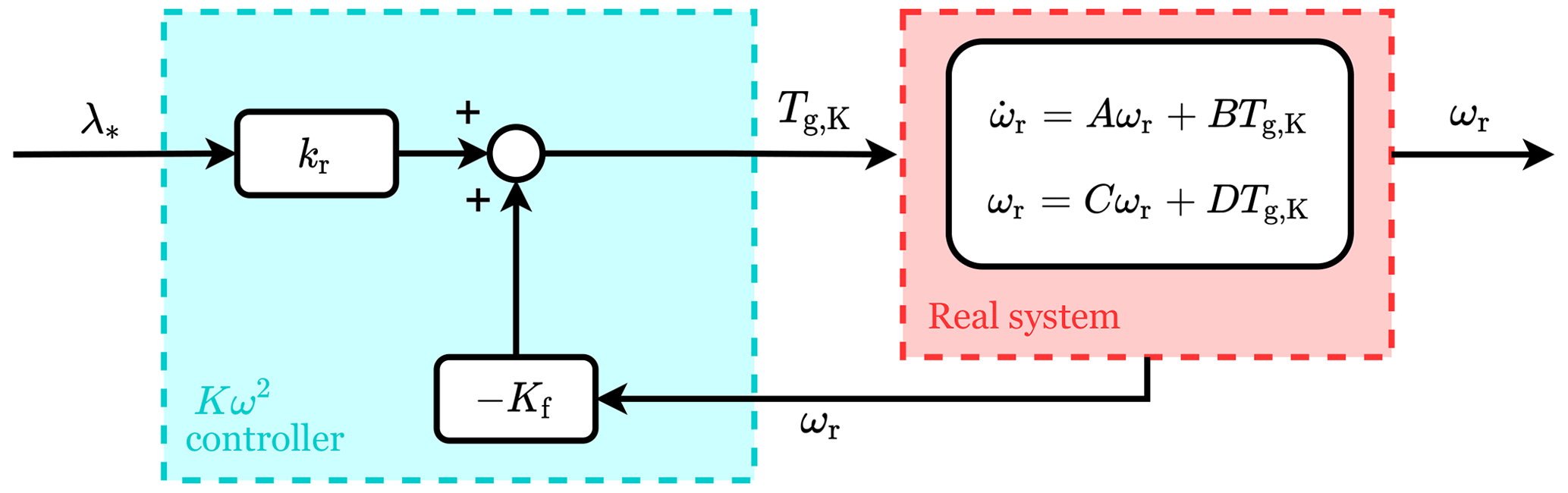
Figure A1 Block diagram of a state feedback controller with a reference shaping block, adapted for the Kω² controller (Aström and Murray, 2010). The full system consists of the real system dynamics, here assumed to be linear, and the controller elements K_f and k_r. The controller uses the system state ω_r and the reference input λ_* to command the wind turbine through its input T_g,K.