Extreme wind turbine response extrapolation with the Gaussian mixture model

The wind turbine extreme response estimation based on statistical extrapolation necessitates using a minimal number of simulations to calculate a low exceedance probability. The target exceedance probability associated with a 50-year return period is $\mathrm{3.8}\times {\mathrm{10}}^{-\mathrm{7}}$, which is challenging to evaluate with a small prediction error. The situation is further complicated by the fact that the distribution of the wind turbine response might be multimodal, and the extremes belong to a different statistical population than the main body of the distribution. Traditional theoretical probability distributions, mostly unimodal, may not be suitable for this task. The problem could be alleviated by applying a fit specifically on the tail of the distribution. Yet, a single unimodal distribution may not be sufficient for modeling diverse wind turbine responses, and an inappropriate distribution model could lead to significant prediction errors, including bias and variance errors. The Gaussian mixture model, a probabilistic and flexible mixture distribution model used extensively for clustering and density estimation tasks, is infrequently applied in the wind energy sector. This paper proposes using the Gaussian mixture model to extrapolate extreme wind turbine responses. The performance of two approaches is evaluated: (1) parametric fitting first and aggregation afterward and (2) data aggregation first followed by fitting. Different distribution models are benchmarked against the Gaussian mixture model. The results show that the Gaussian mixture model is capable of estimating a low exceedance probability with minor bias error, even with limited simulation data, and demonstrates flexibility in modeling the distributions of varying response variables.

1 Introduction

An accurate low exceedance probability estimation is crucial for the statistical extrapolation of wind turbine responses, especially when limited data are available. The crude Monte Carlo simulation (MCS) requires a large sample size, making it computationally expensive. The extreme response with a 50-year return period is usually extrapolated from 10 min simulations, and estimating the 50-year extreme response corresponds to an exceedance probability $p=\mathrm{3.81}\times {\mathrm{10}}^{-\mathrm{7}}$ from 10 min simulations. The coefficient of variation (c.o.v.) of the MCS estimator is $\sqrt{(\mathrm{1}-p)/\left(pN\right)}$, where N is the sample size (Ditlevsen and Bjerager, 1986). Using crude MCS for analysis with such low probabilities requires at least $\frac{\mathrm{10}}{\mathrm{3.81}\times {\mathrm{10}}^{-\mathrm{7}}}=\mathrm{26}\mathrm{280}\mathrm{000}$ simulations for sufficient accuracy, i.e., a c.o.v. $\approx \sqrt{\mathrm{1}/\mathrm{10}}\approx \mathrm{0.316}$. The ultimate design load assessment procedure prescribed by the International Electrotechnical Commission (IEC) aims at ensuring the structural integrity of the turbine when subjected to rare extreme loading conditions. The standards assume three types of scenarios for simulating such rare events: (1) extreme environmental conditions that result in extreme loads, (2) occurrence of faults potentially combined with extreme environmental conditions, and (3) rare occurrences under normal operation. The last option is represented by design load case (DLC) 1.1. It encompasses loads resulting from site-specific atmospheric turbulence occurring during the turbine's normal lifetime, i.e., the normal turbulence model. It establishes the characteristic load value corresponding to a 50-year return period, which could be obtained by statistical analysis of extreme loading using load extrapolation methods. The design load is then obtained by multiplying the characteristic loads by an appropriate partial safety factor (IEC, 2019). The load extrapolation methods are categorized into two approaches, i.e., (1) parametric fitting first and aggregation afterward (FFAA) and (2) data aggregation first and fitting afterward (AFFA). Unlike crude MCS, both approaches use limited data and rely on statistical extrapolation for low exceedance probability estimation, which will introduce prediction error.

In the FFAA approach, the long-term distribution is obtained by aggregating the short-term distributions weighted by the probabilities of occurrence at different wind speed bins. The long-term distribution F_long term(s|T) of the load response s with simulation time T is a function of the short-term distribution $F_{\mathrm{short}\mathrm{term}}\left(s\right|V_k,T)$ at different wind speeds (IEC, 2019):

$$\begin{array}{}\text{(1)}& F_{\mathrm{long}\mathrm{term}}\left(s\right|T)=\sum _{k=\mathrm{1}}^M{F}_{\mathrm{short}\mathrm{term}}(s|V_k,T)p_k,\end{array}$$

where V_k is the mean wind speed at each wind bin, and

$$\begin{array}{}\text{(2)}& p_k=f\left(V_k\right)\mathrm{\Delta }{V}_k,V_{\mathrm{in}}\le V_{\mathrm{1}}<\mathrm{\dots }<V_M\le V_{\mathrm{out}}\end{array}$$

is the probability of occurrence of each wind bin, with f(V_k) being the probability density of the wind speed. V_in is the cut-in wind speed (usually 3 m s⁻¹), V_out is the cut-out wind speed (usually 25 m s⁻¹), and ΔV_k is the wind speed bin width (usually 2 m s⁻¹). The wind speed is divided into bins within the wind turbine's operational range. At each wind speed bin, 10 min simulations are performed, and the short-term distribution of extreme $F_{\mathrm{short}\mathrm{term}}\left(s\right|V_k,T)$ is fitted. The limitation of this approach is that even though $F_{\mathrm{short}\mathrm{term}}\left(s\right|V_k,T)$ might have different probabilistic behaviors at different wind speed bins, the same type of probability distribution is predefined and adopted for ease of application. The tail distribution might not be modeled well at all wind speed bins as there may be uncertainty in the individual fits of the underlying short-term distributions (Freudenreich and Argyriadis, 2008). The key issue is determining the proper distribution model without knowing the underlying conditional distributions at each wind bin. Different distribution models have different tail behaviors, which could result in different long-term response predictions (Ding and Chen, 2013). The estimated extreme loads have a wide range when using the three-parameter Weibull, Gumbel, generalized extreme value (GEV), and lognormal distributions as conditional distributions (Freudenreich and Argyriadis, 2008; Dimitrov, 2016). An improper distribution could result in a far-off extreme load prediction (Freudenreich and Argyriadis, 2008; Dimitrov, 2016).

In the AFFA approach, the environmental input conditions for the 10 min load simulations are sampled directly from their long-term distributions. Hence the data aggregation happens automatically through the distribution choice. The extreme values from all 10 min simulations are fitted to a single probability distribution for extreme load estimation or exceedance probability calculation. This method is also referred to as the post-processing method (Zhang et al., 2020) and is equivalent to a density estimation approach. It suffers from the same challenge as the FFAA approach, as selecting a proper distribution becomes difficult, especially when the underlying distribution is unknown. An improper distribution selection could introduce large estimation errors and far-off extreme response estimation. As the number of simulations is limited, even though different probability distributions are available, selecting the distribution is challenging. Fit accuracy at the center of the distribution does not guarantee a good extrapolation at the tail, which is more important for extreme load estimation. The wind turbine extreme response distributions could have multiple modes (Yang et al., 2022), whereas distributions like Weibull, Gumbel, GEV, lognormal, etc. are unimodal distributions. Yang et al. (2022) compared the AFFA and FFAA approaches with different distributions but have not resolved the statistical extrapolation issue. A possible solution is to fit only the tail data; e.g., Natarajan and Holley (2008) fitted the tail of wind turbine loads using a Gumbel distribution with a quadratic distortion. Mixture probability distributions (e.g., Weibull–Weibull), as discussed in Jung and Schindler (2017), can be beneficial for accurately modeling an entire multimodal statistical population. However, the varying number of modes in wind turbine response distributions, sometimes exceeding two, poses challenges for both bimodal distributions and fixed-component distributions. These challenges stem from mismatches in mode numbers during distribution fitting using the complete dataset. When relying solely on tail data for distribution fitting, the selection of appropriate mixture probability distribution components and their quantities remains a challenge (e.g., Weibull–Weibull, GEV–Weibull, GEV–lognormal–Weibull).

The Gaussian mixture model (GMM) (McLachlan and Peel, 2000) is proposed in this paper as the distribution function for the AFFA approach. It is a flexible probabilistic model and is widely used for machine learning tasks: clustering (He et al., 2011; Zhang et al., 2021; Weber et al., 2022), classification (Huang et al., 2005; Kim and Kang, 2007; Permuter et al., 2006), and image segmentation (Nguyen and Wu, 2013; Yin et al., 2018; Gupta and Sortrakul, 1998). GMM has also been used in the field of wind energy, e.g., wind speed probability density estimation (Wahbah et al., 2018), wind power ramps (Cui et al., 2018), wind turbine power (Zhang et al., 2019), wind turbine power curves (Srbinovski et al., 2021), and environmental contour estimation (Zhang and Natarajan, 2022). GMM is a mixture model whose probability density function (PDF) is multimodal, which is suitable for modeling the multimodal distribution of wind turbine responses. However, its potential in wind turbine extreme response estimation is yet to be explored. The objective of the present paper is to use GMM for extreme response estimation and especially for response variables whose distribution is multimodal. Comparison will be made against using other distributions within the scope of the FFAA and AFFA approaches. The prediction error, which includes bias error (the difference between mean prediction and true value) and variance error (the variability of the prediction), will be systematically investigated on different wind turbine responses.

2 Gaussian mixture model

GMM is a weighted sum of Gaussian distribution components, where each component is defined by its mean (μ) and standard deviation (σ).

The PDF of a GMM is

$$\begin{array}{}\text{(3)}& y\left(x\right)=\sum _{j=\mathrm{1}}^m{\mathit{\pi }}_j\mathcal{N}\left(x|{\mathit{\mu }}_j,{\mathit{\sigma }}_j\right),\end{array}$$

where $\mathcal{N}\left(x|{\mathit{\mu }}_j,{\mathit{\sigma }}_j\right)$ is the PDF of a normal distribution, m is the number of components, and π_j is the component coefficient (weight) and follows

$$\begin{array}{}\text{(4)}& \sum _{j=\mathrm{1}}^m{\mathit{\pi }}_j=\mathrm{1},\mathrm{0}\le {\mathit{\pi }}_j\le \mathrm{1}.\end{array}$$

For a given number of components, the model parameters $\mathit{\{}{\mathit{\pi }}_j,{\mathit{\mu }}_j,{\sum }_j,j=\mathrm{1},\mathrm{2},\mathrm{\dots },m\mathit{\}}$ could be estimated from a dataset whose size is denoted by N, {$x_n,n=\mathrm{1},\mathrm{2},\mathrm{\dots },N\mathit{\}}$ (see Appendix B for more details). The number of components is unknown a priori and should also be estimated from data. It balances the model to prevent underfitting or overfitting. The Akaike information criterion (AIC) (Akaike, 1998) could be used for estimating the optimal number of components m. The method stems from information theory and is an extension of a maximum likelihood estimation with the expression

$$\begin{array}{}\text{(5)}& \text{AIC}=\mathrm{2}k-\mathrm{2}\mathrm{\ell }\left(\mathit{\theta }\right|x),\end{array}$$

where $k=\mathrm{3}m-\mathrm{1}$ is the number of parameters. m and $\mathit{\theta }=\mathit{\{}{\mathit{\pi }}_j,{\mathit{\mu }}_j,{\mathit{\sigma }}_j,j=\mathrm{1},\mathrm{2},\mathrm{\dots },m\mathit{\}}$ that give the minimum AIC value correspond to the optimal number of components and the associated model parameters respectively.

As a mixture model, GMM with two or more components is not Gaussian distributed anymore and has different tail behavior compared to the Gaussian distribution. As its number of components and the associated component coefficients adapt to data, GMM possesses more flexibility than other parametric distribution models. However, it is important to note that when the sample size is small, too many components in GMM may result in an overrepresentation of the data and may compromise its extrapolation capability.

3 Problem formulation and methods

The wind turbine time domain analysis is time-consuming and requires a lot of computational resources, and the feasible number of simulations is often limited. The low exceedance probability is usually extrapolated from a small dataset. Statistical extrapolation thus reduces the number of simulations but introduces prediction errors simultaneously. The prediction error could be described by the mean squared error (MSE) of the estimator ${\widehat{P}}_F$; i.e., MSE$\left({\widehat{P}}_F\right)=V\left({\widehat{P}}_F\right)+{\left[B\left({\widehat{P}}_F\right)\right]}^{\mathrm{2}}$(Wackerly et al., 2008), where $V\left({\widehat{P}}_F\right)$ is the variance error, which describes the variability in prediction using different random samples, and $B\left({\widehat{P}}_F\right)=E\left({\widehat{P}}_F\right)-P_F$ is the bias error, which describes the difference between the mean prediction with true value. The variance and bias error, performance indicators of the wind turbine response extrapolation methods, should be examined.

Choosing an inappropriate distribution will undoubtedly increase the bias error in the FFAA and AFFA approaches. Furthermore, even with the same distribution, different estimations of model parameters can yield varying results. Parameter estimation includes but is not limited to (1) the method of least squares (LSs), which estimates the model parameters by minimizing the sum of the squares of the difference between the observed values and the predicted values from a model; (2) maximum likelihood estimation (MLE); and (3) method of moments (e.g., Weibull model parameter estimation, Moriarty et al., 2004). In the FFAA and AFFA approaches, a comparison is made among the GEV, three-parameter Weibull, and lognormal distributions, along with GMM, using different parameter estimation methods. This comparison involves a total of 11 methods:

1. FFAA with GEV, Weibull, and lognormal as short-term distributions (referred to as FFAA, GEV; FFAA, Weibull; and FFAA, lognormal) conditional on wind speeds, where the MLE is used for model parameter estimation.

2. AFFA with the three distributions using MLE and LS for model parameter estimation (referred to as GEV, MLE; Weibull, MLE; lognormal, MLE; GEV, LS; Weibull, LS; and lognormal, LS).

3. AFFA with GMM using AIC and LS for finding the number of components (referred to as GMM, AIC, and GMM, LS).

In the LS-estimated AFFA approaches, GEV (LS), Weibull (LS), and lognormal (LS), only the tail data (above 80 % quantile) are used to fit the theoretical distributions, where the probability of exceedance of the tail data is calculated as P_t. The probability of exceedance of the response variable is then determined as $P_f=\frac{N_{\mathrm{t}}}{N}\times P_{\mathrm{t}}=\mathrm{0.2}\times P_{\mathrm{t}}$, where N_t is the sample size of the tail data, and N is the total sample size. The AFFA approach using LS minimizes the squared difference between the empirical and theoretical probability of exceedances in the logarithmic scale, with weights assigned to each data point. Specifically, for the sorted dataset in ascending order $S=\mathit{\{}{x}_i,i=\mathrm{1},\mathrm{2},\mathrm{\dots },N\mathit{\}}$, the corresponding empirical cdf $\mathit{\{}F{e}_i=(i-\mathrm{0.5})/N,i=\mathrm{1},\mathrm{2},\mathrm{\dots },N\mathit{\}}$, and the weight $\mathit{\{}{w}_i=\mathrm{1}/\sqrt{F{e}_i\times (\mathrm{1}-F{e}_i)}\mathit{\}}$. The residual for the tail data ${\sum }_{i=N-N_{\mathrm{t}}+\mathrm{1}}^N{w}_i\times {\left(\log (\mathrm{1}-F{e}_i)-\log (\mathrm{1}-F(x_i\left|\mathit{\theta }\right))\right)}^{\mathrm{2}}$ is minimized to get the model parameter θ. Note that the empirical cdf is calculated based on the entire dataset, but the squared error is minimized only on the tail data.

Determining the appropriate number of components of a GMM requires further research. In Eq. (5), AIC is used (referred to as GMM, AIC), where the first term is a penalty term, which discourages overfitting a model, thus balancing model complexity. However, in cases where the sample size is large, the penalty term becomes relatively small, and the AIC approaches maximum likelihood estimation. It will lead to better accuracy at the center of the distribution relative to the tail. To address this, LS on tail data (above 80 % quantile) (shown in the legend as GMM(LS)) is proposed for selecting the number of components m. Following the procedure in Sect. 2, the squares of the residuals from the tail data using GMM associated with the number of components k are calculated (the same as AFFA with LS). The optimal value of m gives the least squares of residuals. Note that the LS here is only for determining the number of components, which is independent of the model parameter $\mathit{\theta }=\mathit{\{}{\mathit{\pi }}_j,{\mathit{\mu }}_j,{\mathit{\sigma }}_j,j=\mathrm{1},\mathrm{2},\mathrm{\dots },m\mathit{\}}$ estimation using the expectation-maximization (EM) algorithm (see Appendix B).

The analysis focuses on four wind turbine responses: (a) the maximum out-of-plane blade tip deflection, (b) the maximum blade root out-of-plane bending moment, (c) the maximum blade root in-plane bending moment, and (d) the maximum tower base side-to-side bending moment. The simulated wind turbine responses are obtained from Barone et al. (2011). To extract peak responses from a sampled time series, the global maxima, block maxima (Fogle et al., 2008; Dai et al., 2022), and peak over threshold methods, average conditional exceedance rates (ACERs) (Naess et al., 2013) could be used (Toft et al., 2011; Dimitrov, 2016; Ding et al., 2013). Different peak extraction techniques will render different results but will not be the focus of this study, where the peaks are obtained using only the global maxima method. The randomness of the responses comes from the wind parameters, where the mean 10 min wind speed is sampled from the Rayleigh distribution, and two random seeds are used for generating the turbulence model. The wind turbine model is a 5 MW NREL reference wind turbine, a three-bladed, upwind rotor with a diameter of 126 m. The FAST aeroelastic code is used for the five million aero-elastic simulations (Barone et al., 2011), which is based on DLC 1.1 in IEC 61400-1 (IEC, 2019).

The 11 methods are firstly compared on the entire dataset with a sample size N∼10⁵. The methods that exhibit relatively small differences compared to the results obtained through crude MCS are further assessed for prediction error, which involves performing statistical extrapolation using 100 sets of smaller sample size samples randomly drawn from the entire dataset. Additionally, for the AFFA approach using the three distributions, the impact of varying amounts of tail data on the results will also be discussed.

4 Results

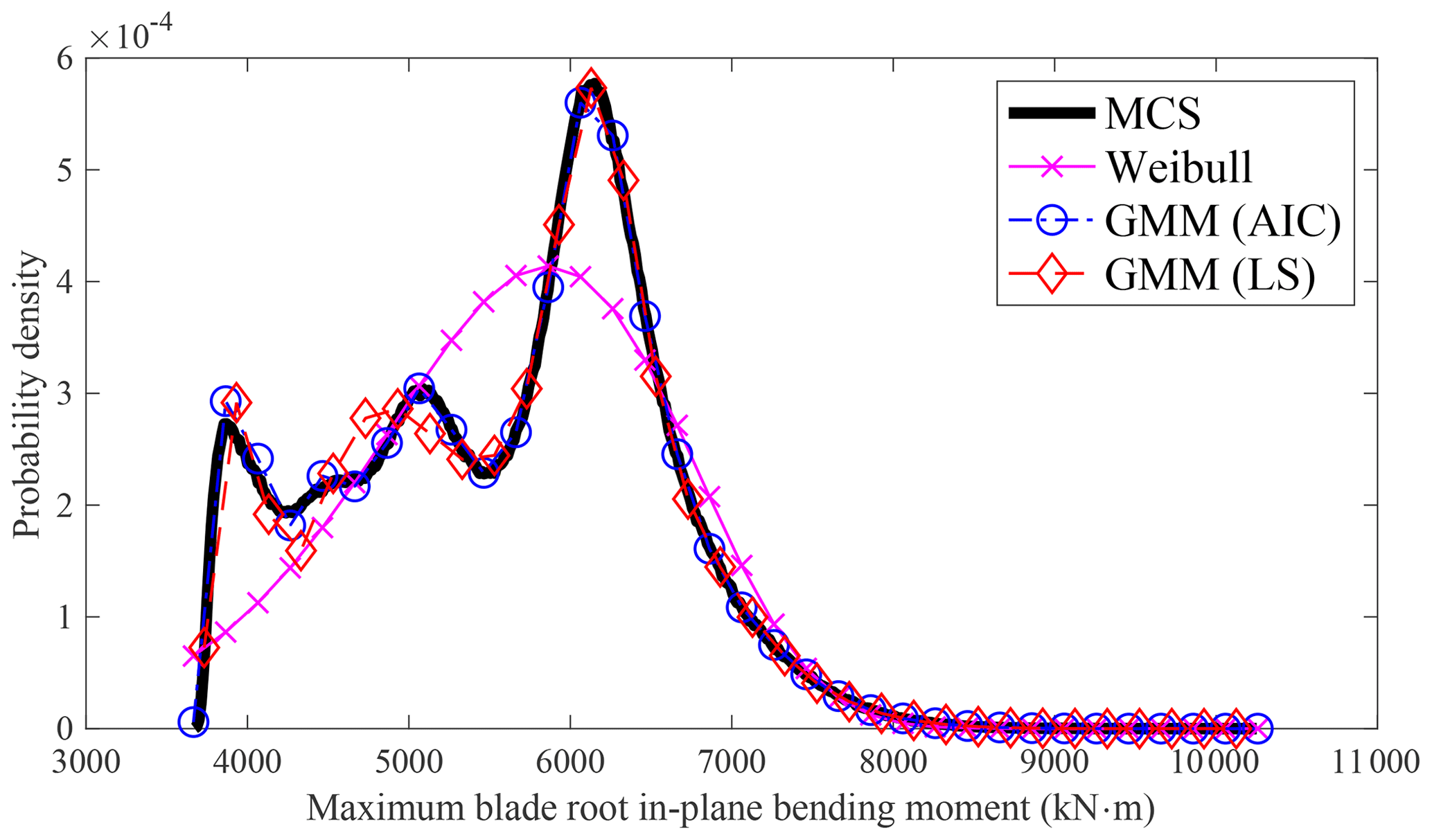
The PDF of wind turbine response (c) from MCS is shown in Fig. 1, which is multimodal. To model the PDF of response (c) using the entire dataset, the Weibull distribution with maximum likelihood estimation is employed. However, as the Weibull distribution is unimodal and cannot capture the multimodal nature of the underlying PDF, a noticeable discrepancy arises between the MCS and the Weibull distribution. Consequently, the Weibull distribution cannot be directly used to model the wind turbine response (c). Similar observations can be made when utilizing other unimodal distributions such as GEV, lognormal, and Gumbel distributions to model other responses. Fitting the wind turbine extreme response with unimodal distributions directly will have a large estimation error at both the center and the tail distribution. This limitation explains why, in the AFFA approach, only the tail portion of the distribution is fitted and utilized for extreme response estimation.

Figure 1 PDF of maximum blade root in-plane bending moment.

4.1 Wind turbine response distribution modeling

The 11 methods are firstly compared on the entire dataset with a sample size N∼10⁵, and the probabilities of exceedance in logarithmic scale are plotted in Fig. 2. Since the predicted exceedance probability already reaches the limit that can be calculated using a Monte Carlo simulation (MCS), this comparison focuses solely on statistical modeling rather than extrapolation.

Figure 2 Probability exceedance estimation with MCS data.

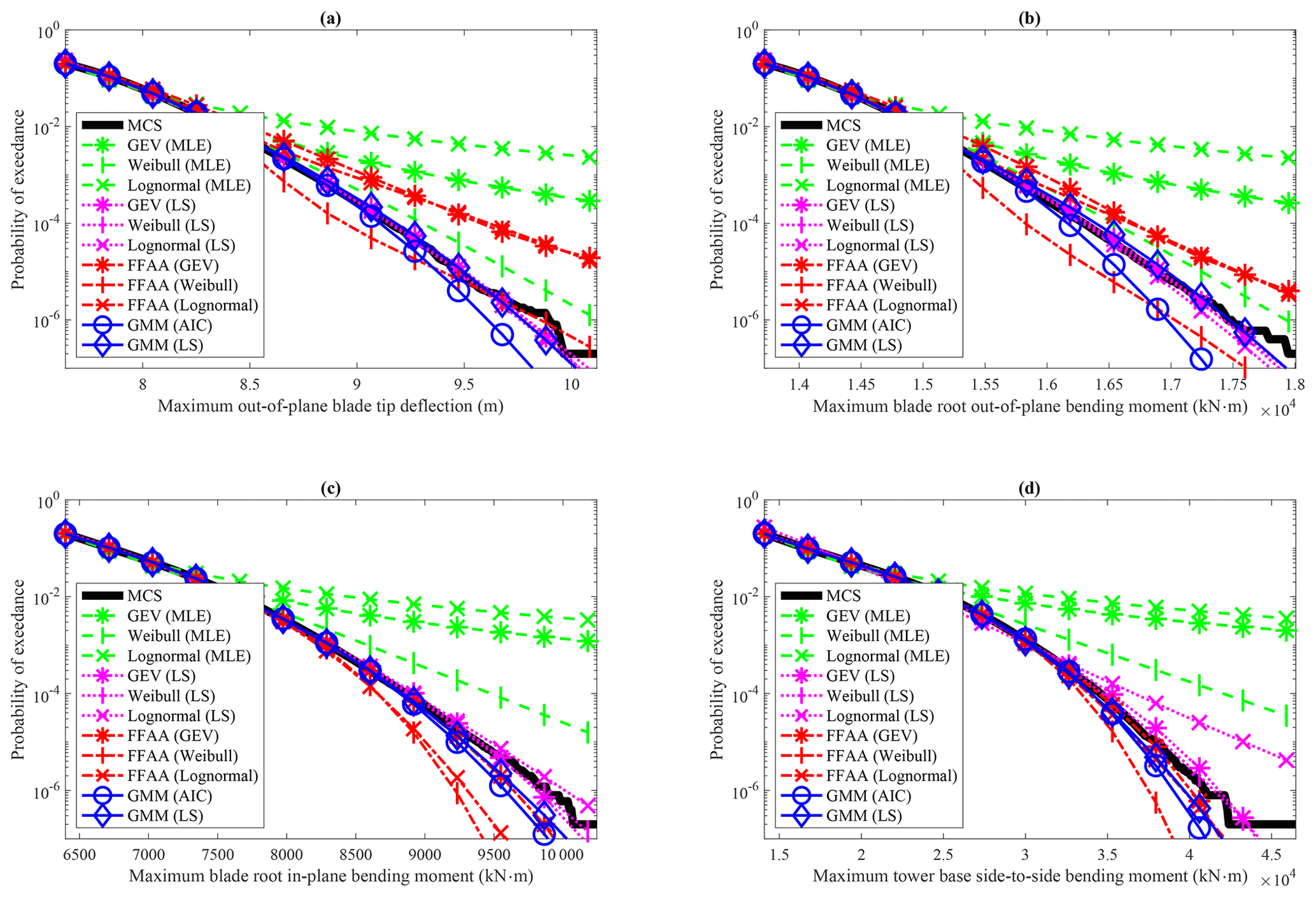
In the FFAA approach, a large difference is observed between the prediction and MCS for cases (a) and (b) regardless of the short-term conditional distribution used. However, when using the GEV distribution for cases (c) and (d) and the lognormal distribution for case (d), a smaller difference is observed. The results indicate that FFAA is a viable option for extreme response estimation, but distribution selection significantly impacts the results.

In the AFFA approach, using MLE for model parameter estimation may not yield favorable outcomes. A significant difference between the prediction and MCS results is observed for all cases, regardless of the distribution used, except for case (b) when using the three-parameter Weibull distribution. Among the three distributions, Weibull consistently performs better than the others regarding tail performance. By focusing only on fitting the tail data and disregarding the accuracy of the distribution at the center, using the LS approach greatly improves the results. For all four cases, the difference between the prediction and MCS is small, except when using the lognormal distribution for case (d), as shown in Fig. 2d. While the choice of distribution has a relatively small effect on the results when using LS for the AFFA approach, it is important to note that an improper distribution selection can still lead to significant deviations in predictions.

Regarding GMM, using LS to determine the number of components outperforms AIC. When the sample size is large, the penalty term in AIC becomes negligible, often resulting in selecting a model with excessive components. In the four cases considered, LS suggests using m=6 components, while AIC suggests using m=9, explaining the difference in performance.

It is important to note that the results shown in Fig. 2 are based on the entire dataset. In practical scenarios, only a relatively small number of simulations can be conducted, and the low probability of exceedance is statistically extrapolated. Since the results of the FFAA and AFFA approaches using MLE for model parameter estimation heavily depend on the choice of distribution, the extrapolation methods employed are compared in the subsequent section.

4.2 Wind turbine response distribution extrapolation

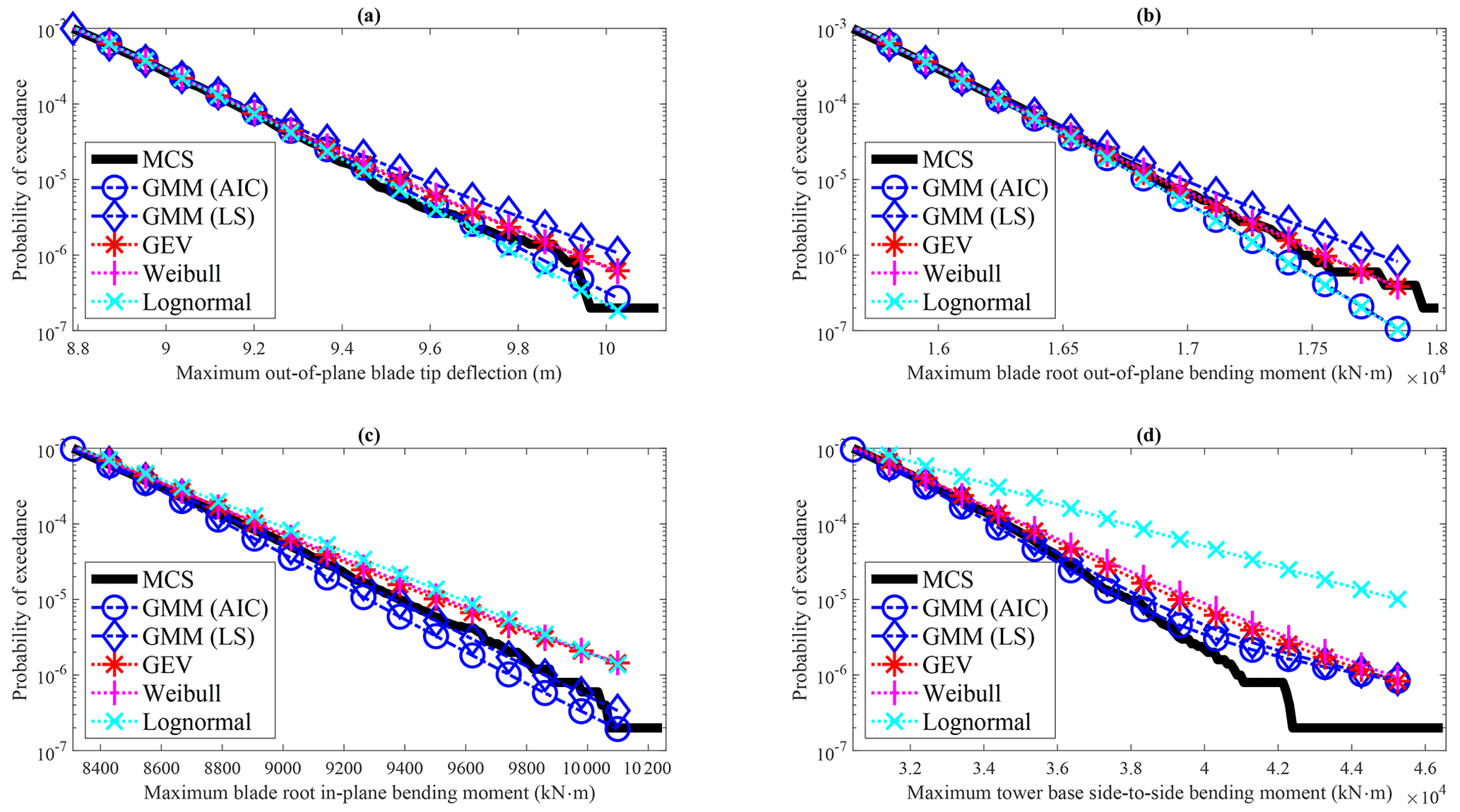
To statistically compare the extrapolation performance of different methods, a random sample of 10⁴ data points is drawn from the entire dataset 100 times. These samples are then utilized for extreme load extrapolation, and the statistical results obtained from each method using these 100 samples are compared. With a sample size of 10⁴, the exceedance probability captured by MCS will not be smaller than 10⁻⁴; thus the statistical extrapolation performance of each method is compared. Given the relatively large distribution modeling errors observed for the FFAA and AFFA with MLE approaches, even when using the entire data dataset, their extrapolation performances are not compared here.

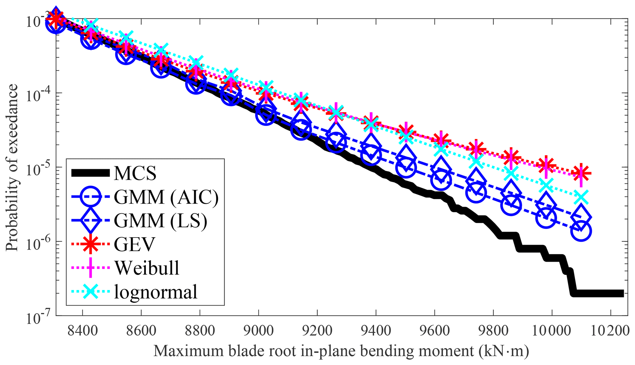
Figure 3 shows the results of the AFFA approach with the GEV, three-parameter Weibull, and lognormal distributions with LS for model parameter estimation, along with GMM using LS and AIC for selecting the number of components. The mean probability of exceedance from 100 samples of each method is plotted, and its difference with MCS represents the prediction bias error. The GEV, Weibull, and lognormal have relatively small bias errors for cases (a), (b), and (c), while they have relatively large bias errors for case (d). Lognormal has the largest bias error for case (d), consistent with the observations made using the entire dataset. On the other hand, GMM has relatively small bias errors for all the cases, except case (d), when the exceedance probability is smaller than $\mathrm{5}\times {\mathrm{10}}^{-\mathrm{6}}$, where it exhibits a relatively larger bias error.

Figure 3 Probability of exceedance estimation with sample data.

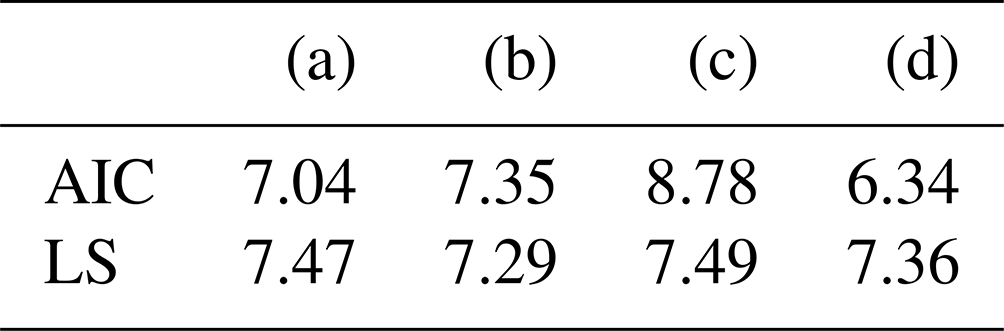
To make further comparisons, especially to examine the variance error in the methods compared, the prediction error at an exceedance probability $P_F=\mathrm{1.90}\times {\mathrm{10}}^{-\mathrm{6}}$, the exceedance probability associated with a 10-year return period, is compared. Assuming ${\widehat{P}}_{F_{\mathrm{MCS}}}$ is the true P_F, the associated extreme response values are obtained as (a) 9.75 m, (b) 1.74×10⁴ kN m, (c) 9.77×10³ kN m, and (d) 4.03×10⁴ kN m for the four wind turbine responses. Several metrics are calculated and presented in Table 1 to compare the performance of the methods at these response locations. These metrics include the following:

• the mean of predicted exceedance probability, denoted as $E\left({\widehat{P}}_F\right)$;

• the variance of the predicted exceedance probability, denoted as V;

• the square of the bias error, denoted as B²;

• the mean squared error, denoted as MSE;

• the root mean square error (normalized by P_F), denoted as $\mathrm{rMSE}/P_F$.

Table 1 Extreme load estimation with sample data.

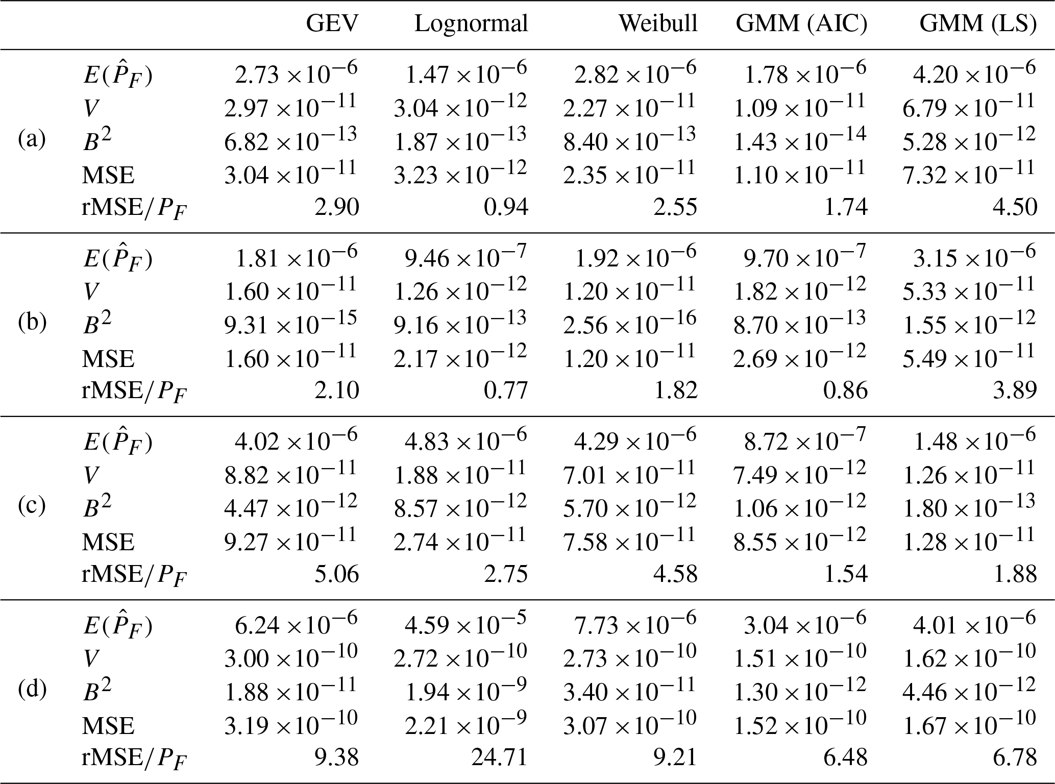
These metrics provide a comprehensive evaluation of the methods in terms of their overall prediction error at the specific exceedance probability of interest.

Except for case (a), it can be observed from both Fig. 3 and Table 1 that the lognormal distribution exhibits a larger deviation in terms of the mean ${\widehat{P}}_F$ compared to the GEV and Weibull distributions. This discrepancy is indicated by the largest bias (B²) value. However, when considering the variance error, the lognormal distribution shows the smallest mean square error (MSE) for the first three cases. This highlights the importance of considering variance errors when making comparisons. Conversely, the lognormal distribution yields the largest MSE for case (d) among all the methods compared. This is due to the distinct tail behavior of case (d), which differs significantly from the lognormal distribution, as it is not sufficiently flexible to fit different response variables.

In contrast, GMM demonstrates considerable flexibility. GMM (AIC) has the smallest MSE for cases (c) and (d) and the second smallest for cases (a) and (b). The distinguishing factor between GMM and other distributions lies in its performance consistency. Given the uncertainty about the underlying data distribution, opting for a flexible distribution with reliable performance, like GMM, becomes advantageous as it mitigates the risk of significant prediction errors caused by an inappropriate model selection. On the other hand, employing the LS method to determine the number of components leads to more prediction errors than AIC in all four cases. This suggests that AIC performs well when the sample size is relatively small. Table 2 provides the average number of components for GMM obtained from the 100 sets when using AIC versus LS.

Table 2 Average number of components for GMM.

In almost all cases, the major contribution to the MSE is V, as compared to B², which shows the importance of considering variance error when performing a statistical comparison. As an exception, in case (d), B² is larger than V, which indicates that lognormal is unsuitable for this particular case as the bias error is excessively large.

4.3 Sample size effect on extreme load extrapolation

The sample size plays a significant role in determining the prediction error for all the methods examined. Van Eijk et al. (2017) investigated the effect of different sample sizes on extreme load predictions and pointed out that the extrapolated 50-year responses could be misleading, and a 300 min time series is not sufficient for 50-year load extrapolation. In the cases discussed above, a sample size of 10⁴ was used to achieve a relatively small prediction error close to the exceedance probability associated with a 10-year return period. Limited by the sample size of the data, the exceedance probability smaller than $\mathrm{1.90}\times {\mathrm{10}}^{-\mathrm{6}}$ is not accurate for MCS and is thus not investigated in this study. Given the time-consuming nature of wind turbine analysis, a smaller sample size is desirable. The results using 100 random samples with a size of 10³ are plotted in Fig. 4. In this analysis, GMM exhibits a relatively smaller bias for $P_F\ge \mathrm{1.90}\times {\mathrm{10}}^{-\mathrm{5}}$, associated with a 1-year return period. On the other hand, for the other three distributions, the bias error becomes quite substantial for exceedance probability smaller than 10⁻³. This demonstrates the limitation of all the compared methods when using a small sample size for extreme response estimation.

Figure 4 Results for case (c) with a sample size of 10³.

5 Discussions

Statistical extreme response extrapolation is important for the probabilistic design of wind turbines. The FFAA and AFFA approaches in IEC 61400-1 (IEC, 2019) are assessed on their modeling and extrapolation performances, where the latter is a more challenging task. The FFAA approach demonstrates feasibility when a suitable short-term distribution is selected, e.g., using GEV as a short-term distribution for cases (c) and (d) (as is shown in Fig. 2). However, it is important to note that the response at each wind speed bin may not follow the same distribution. Consequently, using a single distribution for all bins might introduce prediction errors. Furthermore, different response variables may exhibit different distribution characteristics, and applying a single distribution to various response variables may lead to additional prediction errors. As is evident from Fig. 2, the GEV might perform well for cases (c) and (d) but not the other two response variables.

Flexibility in distribution modeling is important for both the FFAA and the AFFA approaches. The results show that the AFFA approach with LS is less subjected to the effect of choosing distribution models. However, an improper distribution will introduce prediction error. This could be seen from the examples above that using lognormal distribution for case (d) will have a large bias error. Given that wind turbine response variables can exhibit multimodal distributions, it is recommended to utilize a flexible distribution model. GMM fulfills this requirement, making it suitable for extreme response extrapolation. GMM offers the advantage of capturing the multimodal nature of wind turbine responses and can provide more accurate predictions than other distribution models. Therefore, GMM is recommended for modeling and extrapolating extreme wind turbine responses. There are several advantages to using GMM for extreme response estimation:

1. GMM can effectively model both the center and the tail distribution. Figure 1 illustrates that GMM is capable of capturing the bimodal nature of the probability distribution well. In contrast, other unimodal distributions struggle to model the PDF well, making them unsuitable for direct use in extreme response estimation.

2. GMM is a flexible modeling approach that can be applied to different types of wind turbine responses. It consistently performs well across all the compared wind turbine responses. In contrast, other distribution models may perform well for certain response variables but exhibit significant prediction errors for others. For instance, as shown in Fig. 3 and Table 1, the lognormal distribution performs well for the first three cases but demonstrates the largest prediction error for the last case.

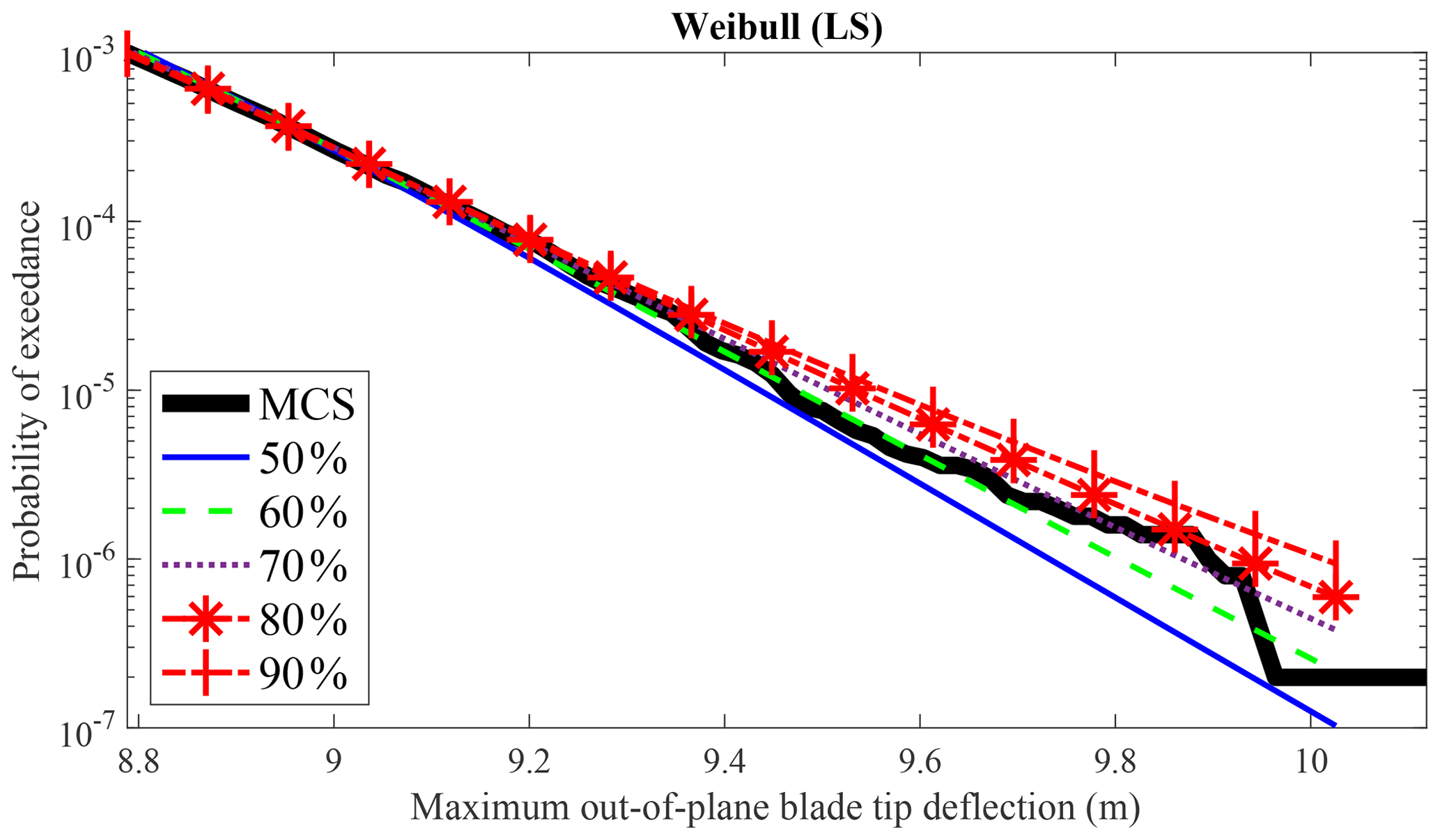
3. GMM eliminates the prediction error associated with selecting different percentages of data for tail estimation. Only the tail data are utilized when fitting the three distributions using the LS method. However, the amount of tail data selected for estimation can lead to varying results. GMM (LS) overcomes this limitation as LS is only used to determine the number of components and is not affected by the choice of quantiles. For example, in Fig. 5, the extreme load estimation for the maximum out-of-plane blade tip deflection is compared using Weibull (LS) with data above the 50th (shown in the legend as 50 %) to 90th (shown in the legend as 90 %) quantiles. Significant differences are observed when using different amounts of tail data for LS with the Weibull distribution.

Figure 5 Results with different quantiles.

In summary, the advantages of using GMM for extreme response estimation include its ability to accurately model both the center and the tail distribution, its flexibility in handling different response variables, and its avoidance of prediction errors associated with selecting different amounts of tail data. These benefits make GMM a recommended choice for wind turbine extreme response extrapolation.

Statistical extrapolation is a challenging problem, particularly when dealing with smaller sample sizes for lower exceedance probability extrapolation. With a sample size of 10⁴, GMM has a noticeable bias error when the exceedance probability is smaller than $\mathrm{5}\times {\mathrm{10}}^{-\mathrm{5}}$ for case (d), as depicted in Fig. 3. It is important to note that when using a smaller sample size, the prediction error is expected to increase, as illustrated in Fig. 4. Thus, caution must be exercised when performing statistical extrapolation, and further research should focus on error analysis in statistical extrapolation. For instance, it would be valuable to investigate the relationship among the sample size, the desired prediction error, and the extrapolated exceedance probability.

It should be mentioned that the favorable performance of GMM in the aforementioned examples is attributed to the underlying distribution being multimodal. For unimodal variables, a flexible univariate distribution could be used for extreme response estimation, e.g., the distribution based on maximum entropy with fractional moments (Zhang et al., 2020). Therefore, the choice of an appropriate distribution should be guided by the characteristics of the variable being analyzed.

6 Conclusions

Extreme response estimation can be likened to low exceedance probability estimation with limited simulations. Both parametric fitting first and aggregation afterward and data aggregation first and fitting afterward approaches could be used for the task. Both approaches with maximum likelihood estimation are quite sensitive to the distribution chosen, which could lead to biased results with an improper probability distribution. The data aggregation first and fitting afterward coupled with least square estimation for fitting the tail distribution is less sensitive to the type of probability distribution. However, an improper probability distribution could still introduce a large prediction error.

There are flexible distributions available, but most are limited to unimodal distribution. The probability distribution of the wind turbine responses could be multimodal. Using unimodal distribution, e.g., GEV, Weibull, and lognormal, to directly fit the distribution for extreme response estimation is infeasible. The Gaussian mixture model is a multimodal distribution by nature and is proposed here for extreme load estimation when the underlying distribution is multimodal. It could model both the center and the tail distribution, is flexible enough for different response variables, and does not require subjectively choosing the threshold compared with the least square estimation of tail distribution. It is thus recommended as an alternative distribution of wind turbine extreme response estimation.

Statistical extrapolation is challenging, and extreme caution must be exercised when making assumptions far beyond the available dataset. Given that the extreme response associated with a 50-year return period necessitates low exceedance probability estimation, an adequate number of simulations is critical for accurate prediction.

Appendix A: Nomenclature

AFFA: Data aggregation first and fitting afterward AIC: Akaike information criterion FFAA: Parametric fitting first and aggregation afterward GEV: Generalized extreme value GMM: Gaussian mixture model LS: Least squares MCS: Monte Carlo simulation MLE: Maximum likelihood estimation PDF: Probability density function

Appendix B: GMM model parameter estimation

The initial model parameters are calculated from the clusters evaluated by the k-means clustering algorithm (Arthur and Vassilvitskii, 2007) and optimized by the expectation-maximization (EM) algorithm (McLachlan and Peel, 2000) as follows:

1. Divide the N data points into k clusters using the k-means clustering algorithm. Compute μ_j, σ_j, and π_j using the data points within each cluster as the initial model parameters for the expectation-maximization (EM) algorithm.

2. EM algorithm

   The model parameters $\mathit{\{}{\mathit{\pi }}_j,{\mathit{\mu }}_j,{\mathit{\sigma }}_j,j=\mathrm{1},\mathrm{2},\mathrm{\dots },m\mathit{\}}$ are found by an iterative EM algorithm (Dempster et al., 1977) to have a maximum likelihood estimation.

   • a.

     E step

     Evaluate the responsibilities using the current model parameters. The responsibility γ_j(x_n) is the probability that component j takes for explaining the observation x_n, which is calculated as

     $$\begin{array}{}\text{(B1)}& {\mathit{\gamma }}_j\left(x_n\right)={\displaystyle \frac{{\mathit{\pi }}_j\mathcal{N}\left(x_n|{\mathit{\mu }}_j,{\mathit{\sigma }}_j\right)}{{\sum }_{i=\mathrm{1}}^m{\mathit{\pi }}_i\mathcal{N}\left(x_n|{\mathit{\mu }}_i,{\mathit{\sigma }}_i\right)}}.\end{array}$$
   • b.

     M step

     Update the model parameters using the responsibilities from the E step. The mean for component j is calculated as

     $$\begin{array}{}\text{(B2)}& {\mathit{\mu }}_j={\displaystyle \frac{{\sum }_{n=\mathrm{1}}^N{\mathit{\gamma }}_j\left(x_n\right)x_n}{{\sum }_{n=\mathrm{1}}^N{\mathit{\gamma }}_j\left(x_n\right)}}.\end{array}$$

     The standard deviation for component j is calculated as

     $$\begin{array}{}\text{(B3)}& {\mathit{\sigma }}_j=\sqrt{{\displaystyle \frac{{\sum }_{n=\mathrm{1}}^N{\mathit{\gamma }}_j\left(x_n\right)(x_n-{\mathit{\mu }}_j{)}^{\mathrm{2}}}{{\sum }_{n=\mathrm{1}}^N{\mathit{\gamma }}_j\left(x_n\right)}}},\end{array}$$

     and the j component coefficient is calculated as

     $$\begin{array}{}\text{(B4)}& {\mathit{\pi }}_j={\displaystyle \frac{\mathrm{1}}{N}}\sum _{n=\mathrm{1}}^N{\mathit{\gamma }}_j\left(x_n\right).\end{array}$$

3. Repeat step 2 until the model parameters converge or the maximum number of iterations is met.