Quantifying the effect of low-frequency fatigue dynamics on offshore wind turbine foundations: a comparative study

Offshore wind turbine support structures are fatigue-driven designs subject to a wide variety of cyclic loads from wind, waves, and turbine controls. While most wind turbine loads and metocean data are collected at short-term 10 min intervals, some of the largest fatigue cycles have periods over 1 d. Therefore, these low-frequency fatigue dynamics (LFFDs) are not fully considered when working with the industry-standard short-term window. To recover these LFFDs in the state-of-the-industry practices, the authors implemented a short- to long-term factor applied to the accumulated short-term damages while maintaining the ability to work with the 10 min data. In the current work, we study the LFFD impact on the damage from the fore–aft and side–side bending moments and the sensors' strain measurements and their variability within and across wind farms. While results might vary strongly between sites, for the current site and a stress–life (SN) curve slope of m=5, up to 65 % of damage is directly related to LFFDs.

1 Introduction

In the next decade, several European offshore wind farms will start approaching their end of as-designed service life (Archer et al., 2014). As a result, the industry must prepare for making complex decisions such as lifetime extension, repowering, optimizing, or decommissioning (Pakenham et al., 2021). A viable option to support this decision would be using structural health monitoring (SHM), through which it is possible to update the as-designed lifetime figures with in situ data. To this aim, strain sensors are installed at the tower–transition piece interface to measure the strains, collecting the support structure's strain over an extended period of up to several years. The strain data, as well as other sources of operational and environmental data, are commonly stored as segmented datasets in 10 min blocks (short term) to be consistent with the duration of design load case (DLC) time series defined and used in the design phase (DNV, 2016). Time series are commonly cycle counted into a histogram through standardized algorithms (ASTM International, 2017), among which rain flow (Amzallag et al., 1994; Socie, 1992) is the most commonly used. The cycle-count histogram summarizes the mean-range (or mean-amplitude) couples and their cycle counts (i.e., the frequency of occurrence within the considered time window).

One cycle represents a closed hysteresis loop in the time series, while a half cycle, also known as residual, is part of a hysteresis loop that did not have the time to complete within the time window. When analyzing signals, it is important to consider the length of the time window used for analysis. Ideally, an infinitely long signal would not have any residuals. However, when working with finite-length signals, residuals can appear with a frequency of at least 1 divided by the time window length (Sutherland, 1999). Therefore, in the industrial approaches, if we analyze multiple 10 min long signals separately, we may obtain different results compared with analyzing a concatenated signal that spans a longer period. This is because the longer period may reduce the impact of residuals on the analysis. This poses a challenge when considering the low-frequency fatigue dynamics (LFFDs) of a (offshore) wind turbine primarily caused by the slow variations in wind speed and direction, which have periods well beyond the default 10 min window.

In this paper, we are interested in the additional damage that might remain unnoticed if the LFFD impact is not taken into account in common practices, such as the commonly used recommended practice (DNV, 2019) for the structural design of offshore wind turbines. Our research intends to provide practical industrial applications, so it must follow the most frequently used industry norms for predicting fatigue lifetimes.

When processing 10 min long signals, these LFFDs cannot be captured, and any possible fatigue damage calculation rule (e.g., linear Palmgren–Miner; Ciavarella et al., 2018; Miner, 1945; Palmgren, 1924) or non-linear models (Hectors and De Waele, 2021) will result in possibly non-conservative fatigue life estimates as some of the largest cycles remain unaccounted for. On the other hand, concatenating the segmented signals and cycle counting the output are of very little practical applicability, given that there could be multiple years of SHM data sampled at frequencies well above 1 Hz (D'Antuono et al., 2022), and results can no longer be matched with the 10 min design load cases (DLCs). To consider the LFFD effect, some researchers have adopted various strategies.

One idea is to count half cycles as full cycles, but this would not cover the whole effect of the LFFD. In fact, counting residuals as full cycles is not a common practice as it does not have any physical rationale, as there is no hysteretic loop being artificially closed. Based on the IEC standard (IEC, 2001), it is recommended to treat half cycles as half cycles.

Because of the potential discrepancy, some research on the role of LFFDs in wind energy has been conducted. On a small wind turbine (Micon M150), Larsen and Thomsen (1996) established and used a framework for an approximative treatment of low-frequency contributions. They demonstrated that the low-frequency part of the blade flapwise moment accounts for roughly 8 % and 1 % for large and small Basquin slopes in terms of equivalent moments. For large and small Basquin slopes, the low-frequency portion contribution to the corresponding moment for the rotor tilt is roughly 2 % and 0.4 %. When considering the LFFD effect of a Vestas V90-2.0 MW wind turbine, Pacheco et al. (2022) reported that the damage calculated with a trilinear SN curve from Eurocode 3 and from a 24 h time series was 11 % higher than the damage obtained with a 10 min time series.

The present paper adopts an algorithm that allows for recovering the LFFD through the sequences of residuals of the segmented data and their cycle-count histograms. The algorithm was first proposed by Amzallag et al. (1994), and then Marsh et al. (2016) applied it specifically to wind energy on a multi-megawatt offshore wind turbine. For m=3 and m=5, Marsh et al. (2016) reported an increase of up to 10 % and 170 %, respectively, in the final damage when LFFD was accounted for. Finally, Sadeghi et al. (2022) validated the procedure using 3 years of SHM data coming from an offshore wind turbine monopile foundation. In that work, the LFFD recovery algorithm was used to calculate an LFFD factor that, once applied to the sum of the damages from each short-term dataset, allows the recovery of the detrimental effect of the low-frequency and high-range fatigue cycles.

The LFFD factor is equal to the ratio of the damage calculated using long-term data to the damage calculated using short-term data. Both Marsh et al. (2016) and Sadeghi et al. (2022) have found that the said factor converges to a fixed value after a specific amount of time, suggesting that once the LFFD factor is converged there is no need to continue to work with long-term cycle counting. Moreover, the LFFD factor provides direct insight into the relative importance of LFFDs on overall fatigue.

The LFFD factor will play a role in assessing the fatigue life of operational offshore wind turbines (OWTs) to account for the long-term cycles to which the support structure is subjected and meanwhile collect data in 10 min windows, far better suited for comparing with DLCs or fatigue prognoses (Noppe et al., 2020). However, Marsh et al. (2016) have already showed that the LFFD factor is highly dependent on the gradient of the chosen SN curve. Moreover, the LFFD factor presumably depends on the stress history, which is site-, turbine-, and even sensor-specific, as the number and size of LFFD cycles will depend on the prevailing environmental and operational conditions. This work investigates the behavior of the LFFD factor under various scenarios using strain measurements from several OWTs.

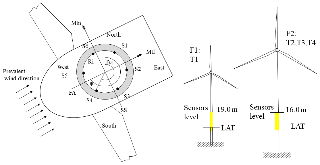
Figure 1 Schematics of the instrumentation setup for Farm 1 and Farm 2. Sensors are installed at the tower–transition piece interface level.

2 Measurement setup and methodology

The OWI-Lab had access to data of four OWTs across two wind farms which were geographically close to each other, with near-identical metocean conditions. The first farm includes one of the first generations of 3 MW OWTs, while the second farm has a larger and newer generation of 9 MW OWTs, installed in deeper waters and with larger rotor diameters compared with the first wind turbine in Farm 1. While both farms used monopile foundations, the larger monopiles in Farm 2 have a far larger impact from wave-loading-induced fatigue compared with the smaller monopile at Farm 1, as the larger wind turbines have lower natural frequencies, closer to the wave spectra (Laszlo et al., 2016). We have 3 years of data for one turbine (Farm 1), while for the remaining three wind turbines (Farm 2), we have collected 1 year of data. As shown in Fig. 1, each turbine is equipped with six longitudinal strain gauges mounted 60^∘ apart and installed at the tower–transition piece interface, 16 and 19 m above the lowest astronomical tide (LAT). The three turbines of Farm 2 (F2) have similar models and structural designs. The heading (position) of strain sensors along the circumference of the tower is almost similar for all four turbines. Also, the dominant wind direction, which was almost similar for the four turbines, is shown in this figure. Sensors S2 and S4 of Turbine 1 and S6 of Turbine 3 were faulty and were neither used to calculate bending moments nor used to calculate the heading-specific damage.

From the strain measurements at the sensors (S1 to S6), we can calculate stresses (σ) and bending moments (M) at any location in the structure through Hooke's law (Eq. 1) Navier's formula for axial stress (Eq. 2), and a rotation matrix (Eq. 3):

$$\begin{array}{}\text{(1)}& {\displaystyle }{\mathit{\sigma }}_{zz,j}=E{\mathit{\epsilon }}_{zz,j},\text{(2)}& {\displaystyle }\begin{array}{rl}{\mathit{\sigma }}_{zz,j}& ={\displaystyle \frac{F_{\mathrm{N}}}{A}}+R_{\mathrm{i}}\cdot [{\displaystyle \frac{M_{\mathrm{north}\text{–}\mathrm{south}}}{I_C}}\cdot \sin \left({\mathit{\theta }}_j\right)-{\displaystyle \frac{M_{\mathrm{east}\text{–}\mathrm{west}}}{I_C}}\\ & \cdot \cos \left({\mathit{\theta }}_j\right)],\end{array}\text{(3)}& {\displaystyle }\begin{array}{rl}\left\{\begin{array}{l}{M}_{\mathrm{tl}}\\ M_{\mathrm{tn}}\end{array}\right\}=& \left[\begin{array}{ll}\cos (-\mathit{\psi }+\mathit{\pi })& \sin (-\mathit{\psi }+\mathit{\pi })\\ -sin(-\mathit{\psi }+\mathit{\pi })& \cos (-\mathit{\psi }+\mathit{\pi })\end{array}\right]\cdot \\ & \left\{\begin{array}{l}{M}_{\mathrm{north}\text{–}\mathrm{south}}\\ M_{\mathrm{east}\text{–}\mathrm{west}}\end{array}\right\},\end{array}\end{array}$$

where E is Young's modulus; ε_zz,j and σ_zz,j are the axial strain and stress at the jth sensor, respectively; F_N is the normal load; θ_j is the clockwise angle between the north–south axis and the jth sensor; R_i is the inner radius of the sensor location; A is its cross-sectional area; I_C is its area moment of inertia; and ψ can be any desired heading. In Eq. (3), ψ is selected as the average yaw angle within a 10 min time window, so the rotation matrix will return the fore–aft (FA) and side–side (SS) bending moments (M_tn and M_tl) for each window.

The authors dealt with the methodology to recover the low-frequency fatigue cycles in detail in a previous study (Sadeghi et al., 2022); therefore, the process is not repeated in this paper. In that work, 3 years of SHM data have been used to demonstrate that concatenating the segmented time signals and cycle counting the resulting signal have the same effect as merging the segmented cycle-count histograms with the cycle-count histogram of the residual sequences from the segmented data. This operation has multiple advantages: (i) it is faster, (ii) it requires less database space, and (iii) it is much more versatile than the short-term signal concatenations (Marsh et al., 2016). The necessary steps to obtain a long-term cycle-count histogram through the LFFD recovery algorithm are described in detail in our previous publication (Sadeghi et al., 2022). The final result is a cycle-count histogram which contains the low-frequency cycles.

Figure 2 SN curves used.

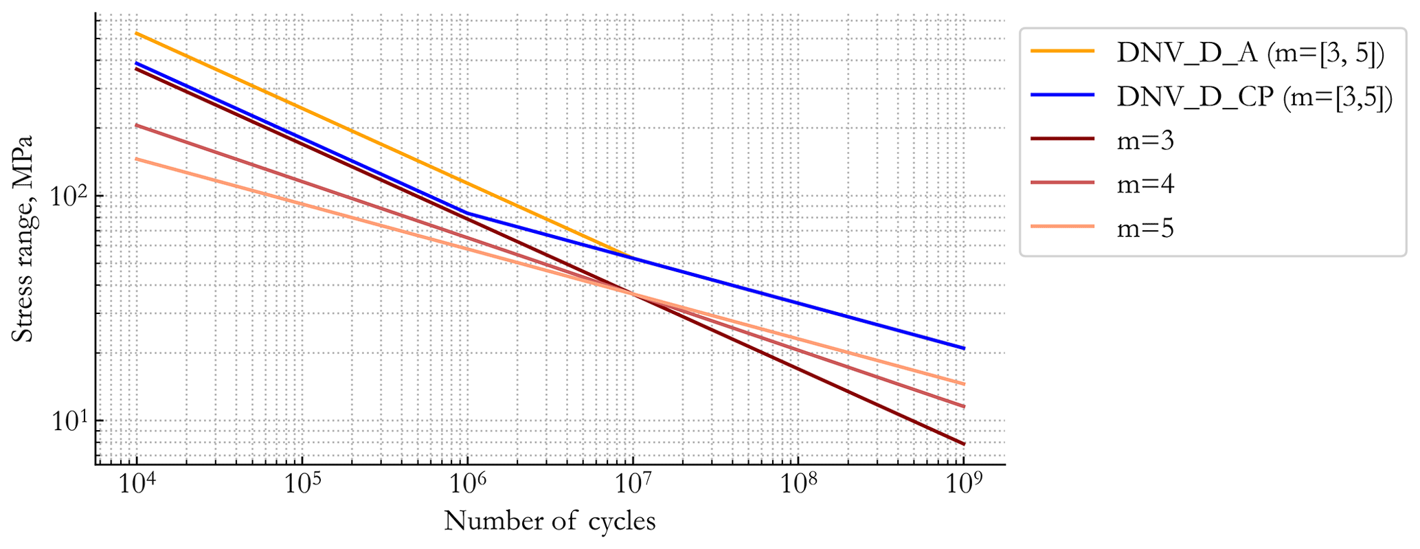
In the current study, the overall fatigue damage with LFFDs is calculated using the Py-Fatigue Python package (D'Antuono et al., 2023) and through the Palmgren–Miner rule (Eq. 5) combined with the stress–life (SN) curve as defined by Basquin's law (Basquin, 1910) (Eq. 4). Although the linear Palmgren–Miner rule is relatively imprecise and does not account for load sequence or memory effects, it is by far the most popular and commonly utilized damage accumulation rule (Ciavarella et al., 2018), required as a safety standard even by safety-critical industries such as aviation transport (EASA, 2020), although more accurate models are available (Hsiao et al., 2021). Following the DNV-RP-C203 guidelines using the single-gradient curves (Iliopoulos et al., 2017), the selected SN curves are illustrated in Fig. 2. We chose three linear SN curves with different slopes (3, 4, and 5) because these are normally used to calculate damage-equivalent moments (DEMs), as one of the applications of the desired LFFD factor would be to consider the LFFD effect in the calculated DEM (refer to Appendix C). The focus on the single-gradient linear SN curves is motivated by the desire to have a general LFFD factor, independent of the fatigue spectra and multiplicative factors. On the other hand, bilinear SN curves will yield to a non-generalizable LFFD factor, as is discussed in Sect. 4.3, using two bilinear SN curves of DNV_D_A and DNV_D_CP, which are the SN curves for detail type D in air and in seawater with cathodic protection, respectively (Iliopoulos et al., 2017). Meanwhile, the seawater with a free corrosion curve is a single-slope SN curve (m=3), and thus the LFFD factor for m=3 applies.

It is worth mentioning that in the current research, for simplicity no existing damage was assumed on the structures, and initially the residuals were counted as half cycles. Furthermore, no mean stress corrections were used, and the loading was assumed to be uniaxial. Both assumptions serve to simplify the outcomes of this analysis while aligning with DNV (2019). As the recommended practice specifies that if the maximum cyclic stress is greater than 0 (overall tension), no mean stress correction shall be applied (factor = 1), while a constant factor < 1 can optionally be used for the stress ranges when residual compressive stresses can be documented.

Similarly, regarding the behavior under combined loading, we again follow the recommended practice (DNV, 2019). As the SN curves used were obtained from specimens that underwent uniaxial tests, we disregard the impact of torsional and shear loads. From a practical point, no data were collected for these loads due to the lack of sensors in those directions.

The short- to long-term fatigue damage LFFD factor is expressed in Eq. (6) as the ratio of the damage from long-term fatigue histograms to the damage from short-term fatigue histograms; i.e.,

$$\begin{array}{}\text{(4)}& {\displaystyle }& {\displaystyle }N\cdot (\mathrm{\Delta }\mathit{\sigma }{)}^m=a,\text{(5)}& {\displaystyle }& {\displaystyle }D=\sum _{j=\mathrm{1}}^{N_{\mathrm{blocks}}}{\displaystyle \frac{n_j}{N_j}}=\mathrm{1}/a\cdot \sum _{j=\mathrm{1}}^{N_{\mathrm{blocks}}}{n}_j(\mathrm{\Delta }\mathit{\sigma }{)}_j^m,\text{(6)}& {\displaystyle }& {\displaystyle }\mathrm{LFFD}\mathrm{\_}\mathrm{factor}=D_{\mathrm{LT}}/D_{\mathrm{ST}},\end{array}$$

where (m, a) are the SN curve slope and intercept, respectively; n_j is the number of cycles in the jth load block; N_j is the cycle to failure at the load level Δσ_j; and D_LT and D_ST are the long-term and short-term fatigue damages. As the number and the stress range of large cycles increase after the LFFD recovery, see Fig. 3, LFFD_factor ≥ 1.

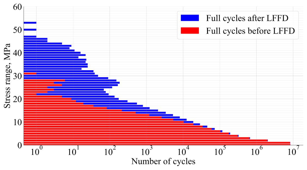
Figure 3 Comparison of full cycles of 1 year of cycle count FA from Turbine 1, before and after applying LFFDs.

Figure 3 shows how the number of full cycles increases after considering the low-frequency cycles. It can be seen that the added full cycles mainly have stress ranges of over 10 MPa, and therefore they will have a large contribution to the final damage.

It is noteworthy that the LFFD factor for single-gradient curves does not depend on the SN curve intercept (a) but the slope (m) only. This is shown in Eq. (7) by substituting Eq. (5) in Eq. (6):

$$\begin{array}{}\text{(7)}& \mathrm{LFFD}\mathrm{\_}\mathrm{factor}={\displaystyle \frac{\sum _{j=\mathrm{1}}^{N_{\mathrm{blocks}}}{n}_{\mathrm{LT},j}(\mathrm{\Delta }\mathit{\sigma }{)}_{\mathrm{LT},j}^m}{\sum _{j=\mathrm{1}}^{N_{\mathrm{blocks}}}{n}_{\mathrm{ST},j}(\mathrm{\Delta }\mathit{\sigma }{)}_{\mathrm{ST},j}^m}}.\end{array}$$

As a consequence, given that $\max \left[\right(\mathrm{\Delta }\mathit{\sigma }{)}_{\mathrm{LT},j}]\ge max[\left(\mathrm{\Delta }\mathit{\sigma }{)}_{\mathrm{ST},j}\right]$, if the slope increases, the effect of the large low-frequency cycles will increase, and the LFFD factor will increase.

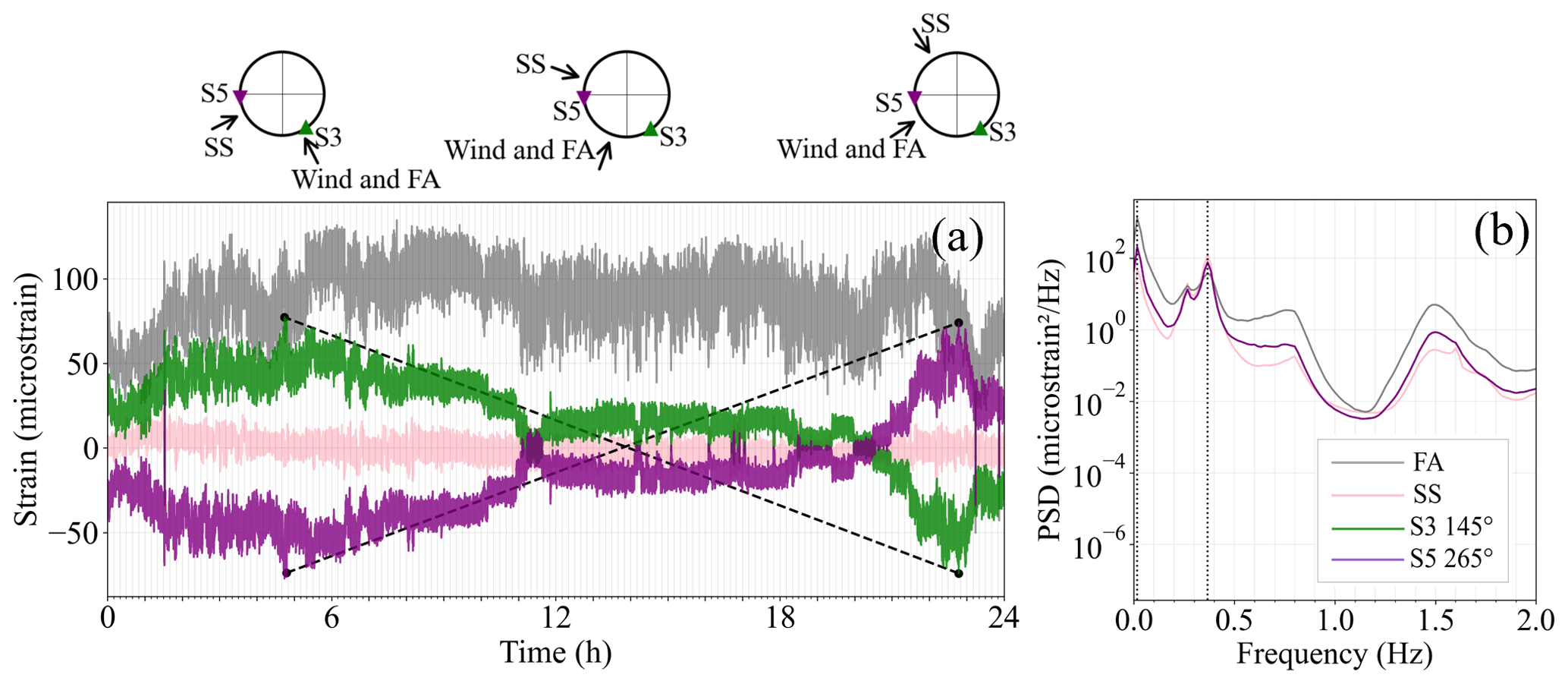
Figure 4 (a) Strain signals of FA, SS, and two sensors. The dashed black lines show the schematic of two LFFD cycles forming during a day from the change in wind speed and direction. (b) The frequency spectrum of FA, SS, and two sensors. The two dotted vertical lines show the first and second modes.

In Fig. 4a, a single day of real-world data collected from Farm 1 are used to show how a low-frequency cycle forms. The measurements for both the FA and the SS bending moments as well as two individual strain gauges are shown against the wind speed and direction. The vertical grid lines show the 10 min short-term windows. For the FA direction, slow variations in the bending moment spanning several hours can be seen. These LFFDs far exceed the cycles observed within a 10 min window and can be directly correlated to the variations in wind speed over the day. Meanwhile, for the SS, the bending moment is not affected by these variations in wind speed.

While the FA bending moment is only affected by the wind speed, a secondary effect can be seen for the individual strain gauges at headings 145 and 265^∘ (S3 and S5). For example, at the start of the day, S3 is in tension as the wind is coming from the southeast (153^∘); meanwhile, S5 is in compression. In the midday, the wind heading is between the two sensors, and therefore their mean strain is around 0. Towards the end of the day, S3 is in compression and S5 is in tension. These LFFD cycles are readily explained when considering that the wind direction has also changed towards the west (237^∘). Examples of two LFFD cycles are shown by the dashed black lines. This illustration suggests that the size of the LFFD effect will vary along with the wind conditions at a site as well as the type of signal considered. Note that in this plot, the sensors' strain is de-trended to have 0 means. In Fig. 4b, the frequency spectrum of the two sensors as well as the FA and SS strain signals are shown. The sensors' frequency plots are overlying. The first highest peak happens at a very low frequency of 0.016 Hz, and FA and SS have the highest and lowest power density, while the sensors' power is in between them. The second dominant frequency is around 0.36 Hz at the frequency of the first dynamic mode, but in this frequency, SS has the largest height, while FA has the least value.

3 Objective

In the present work, we perform an in-depth analysis of the LFFD factors to investigate the variability of the LFFD factor over time, across different sensor positions, locations, and wind farms. We are interested in the additional damage that might be ignored if we do not consider the LFFD effect in common practices. Our work is aimed at practical industrial applications, and, as such, it must adopt the most widely accepted industry practices and standards for fatigue lifetime prediction. In particular, the following is investigated in further detail:

1. the trend of the convergence of LFFD factors over time and the relative importance of growing time horizons in LFFDs

2. comparison of LFFD factors for the direct measurements of sensors along the circumference of the wind turbine support structure with those calculated for FA and SS bending moments

3. multiple support structures (with similar designs) in the same wind farm

4. multiple foundation designs coming from two different wind farms.

The final scope of this study is to define the right short- to long-term fatigue damage LFFD factor for a specific OWT that can be applied as a multiplicative constant to the short-term damage whenever the low-frequency fatigue cycles cannot be retrieved, for instance, when working with 10 min damages or equivalently when working with short-term damage-equivalent loads (DELs), where the time order of the short-term dataset is not available (Hübler et al., 2018; Weijtens et al., 2016).

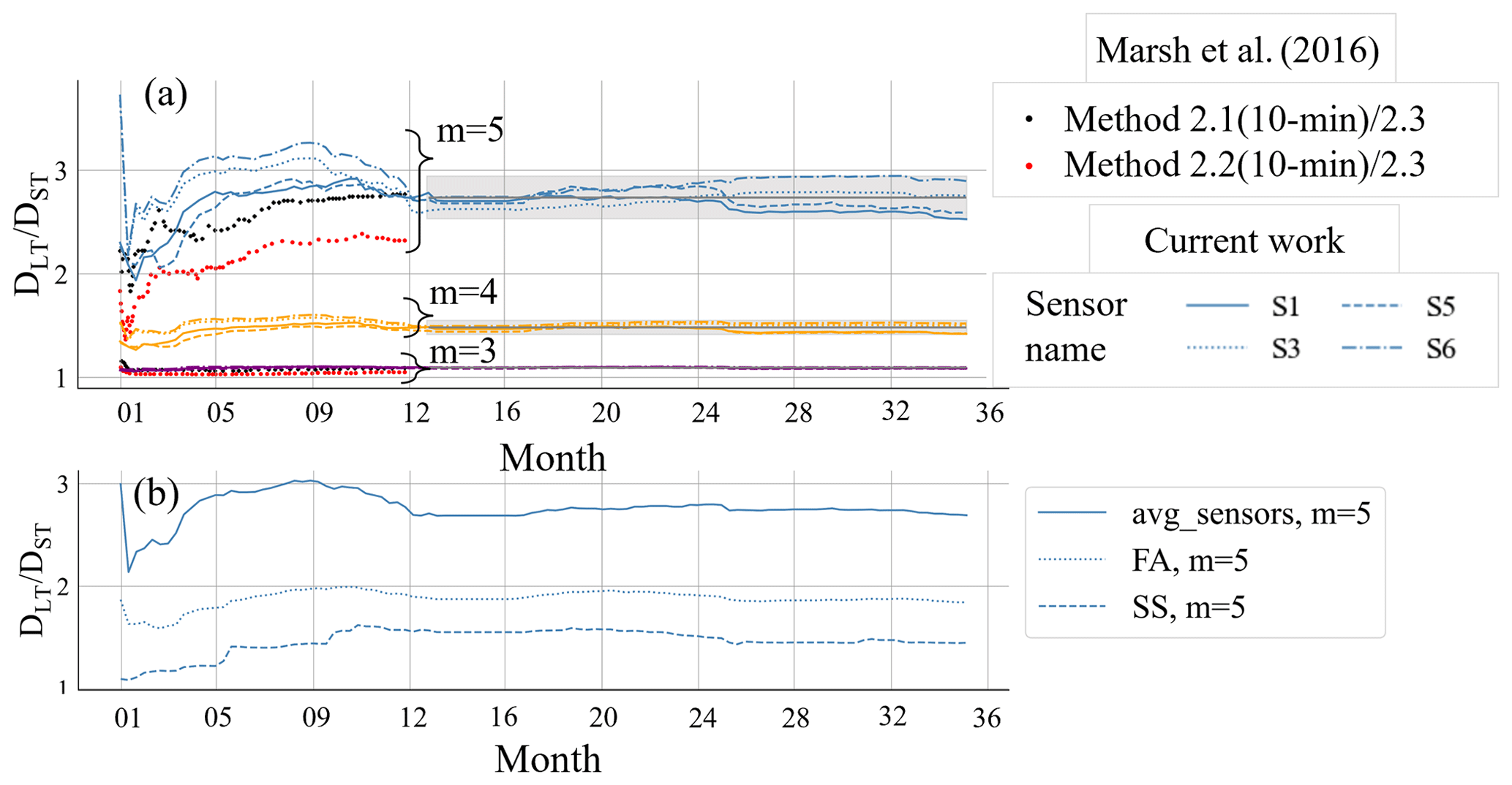
Figure 5 (a) Trend in LFFD factor along the circumference of T1 over time using 3 years of SHM data, plus the results of Marsh et al. (2016). The solid grey line shows the average of the converged values of all sensors, and the grey area is the average ± 2 SDs. (b) Comparison of the LFFD factor value from FA and SS and the average of the sensors for m=5.

4 Case studies

4.1 The behavior of the LFFD factor for FA and SS and sensors and the trend over time

Figure 5a shows the trend in the LFFD factor over time along the circumference (four sensors) of the monopile under consideration (T1) for single-slope SN curves with slopes of m=3, 4, and 5 shown by purple, yellow, and blue lines. Additionally, the results of Marsh et al. (2016), from 1 year of stress data collected from a multi-megawatt offshore wind turbine support structure are plotted for m=3 and 5.

Generally, the factor depends mostly on the SN curve slope (m) rather than the considered strain history. The first stabilization of the LFFD factor appears after 3 months, in agreement with what was found by Marsh et al. (2016), but after almost 6 months, a season-dependent effect causes some variation in the LFFD factor. For this reason, we consider the alternation of four seasons (≥1 year) as the minimum time window that gives a stable value of the LFFD factor. Concerning the influence of the SN curve and the behavior along the circumference, after convergence, the LFFD factor is relatively stable. Its variations can be safely expressed by a mean value of ± 2 SDs (standard deviations) (solid grey line and area in Fig. 5a). Marsh et al. (2016) showed a factor of around 2.3 and 2.7 for m=5 and 1.1 for m=3, which are comparable with the values from the current study. A summary of the information on the converged factors for different SN slopes (m=3, 3.5, 4, 4.5, and 5) for all four turbines is available in Appendix A.

To evaluate the different LFFD factors for FA, SS, and strain of individual sensors, we compared the LFFD factor calculated from the FA and SS bending moments with the average LFFD factor of the sensors of Turbine 1, in Fig. 5b. We only focused on m=5, as it has the highest LFFD factor values. The plot shows that the lowest LFFD factor is found for the SS direction and that the average LFFD factor of the sensors (2.76) is much higher than those found for the FA and SS directions (1.89 and 1.5, respectively). As illustrated in Fig. 4, the likely cause of the larger role of LFFDs for fixed headings is the LFFD cycles caused by the changing wind directions over time. The maximum margin of scatter for the average value of all four sensors (grey line in Fig. 5a) (for m=5) is 0.25. It is equal to 2 standard deviations, which is shown by the grey area.

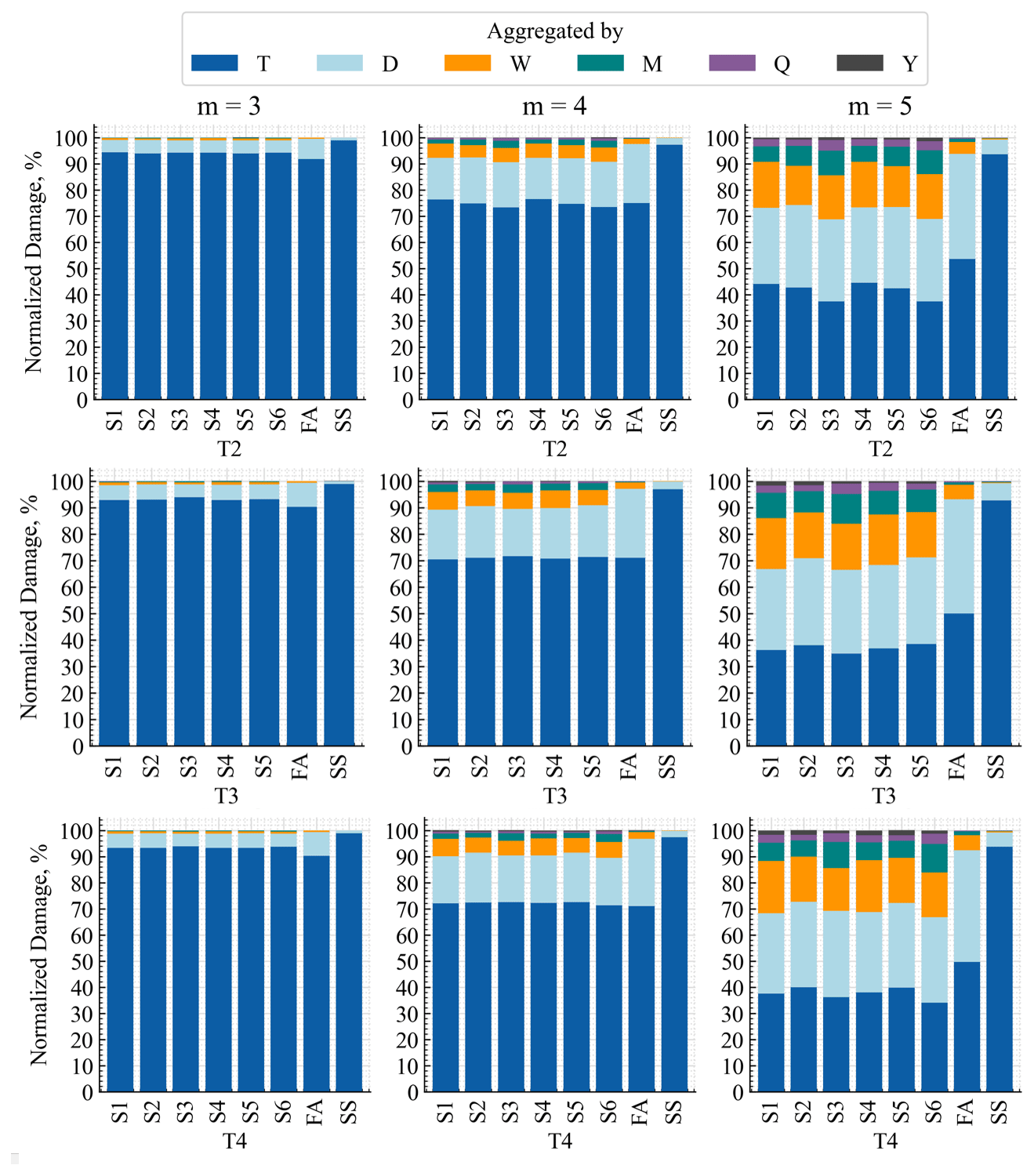
To better understand the mechanism behind the LFFD factors, we calculated the LFFD factors by considering different window sizes over the whole measurement duration: yearly, seasonal, monthly, daily, and 10 min. For example, for the whole duration, all the low-frequency cycles are considered; for yearly (Y) durations, cycles shorter than 1 year are considered; for seasonal (Q) durations, cycles shorter than 3 months are considered; for monthly (M) durations, cycles less than 1 month are considered; for daily (D) durations, cycles shorter than a day are considered; and for 10 min windows, no LFFDs are considered (T). Figure 6 shows the results for damages calculated with the mentioned aggregation windows. The damages are normalized to the “total damage” from cycle counting the entire signal together. The result was valid over both farms and all four turbines; therefore we only show the T1 results. The plots for the other three turbines are in Appendix B.

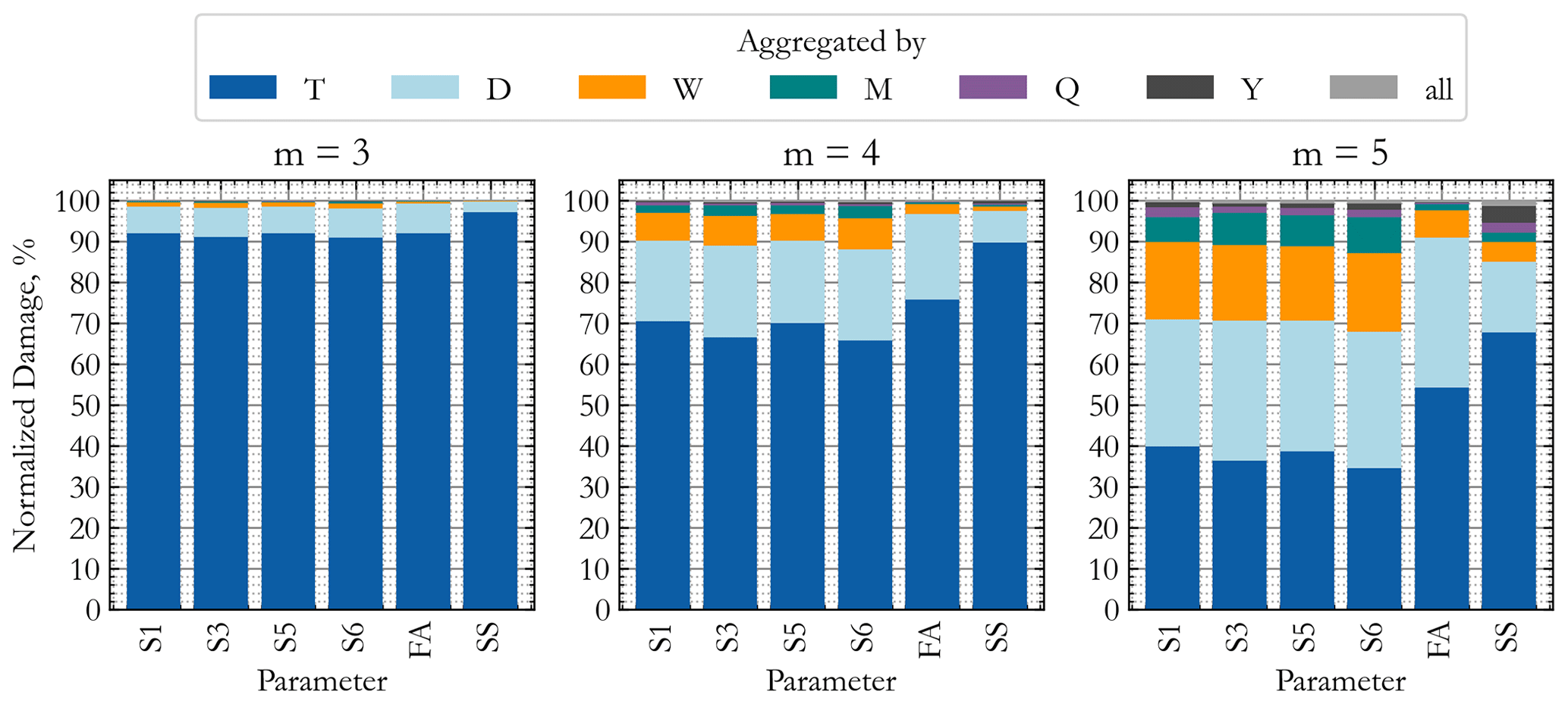
Figure 6 Share of the low-frequency cycles of various lengths in the final LFFD factor of T1 after 3 years. Damages are normalized to 100 %. (Without LFFD: T, daily: D, weekly: W, monthly: M, quarterly: Q, and yearly: Y). Results for the three other turbines are provided in Appendix B.

Note that the LFFD factor(s) are found as 100$/$normalized damage (T). Figure 6 illustrates that for all slopes, daily cycles contribute to the majority of the LFFD factor. For this turbine, we notice that for m=3, cycle counting on a daily basis covers ca. 98 % of the total damage of an individual sensor and in the FA direction. By comparison, for m=4, cycle counting daily only accounts for ca. 90 % of the total damage for individual sensors, while 96 % and 99 % of total damage is accounted for when a weekly and a monthly basis, respectively, is considered. For m=5, cycle counting on a monthly basis covers ca. 96 % of the total damage (of sensors). Results seem to suggest that considering longer periods has trivial added value. The exception is an apparent large contribution of yearly cycles in the SS result for m=5; however, this behavior seems limited to turbine T1 and might be due to an anomalous cycle, e.g., due to a sensor malfunction.

Consistent with Eq. (7), by the increase in the slope of the SN curve, the share of long-term damages and the need to consider a longer time window increase. Among the sensors, S3 and S6, which are normal to the dominant wind direction, have the smallest short-term damage contribution, which translates to the highest LFFD factors.

Comparing the composition of the LFFD for individual sensors against that of the FA and SS directions, we observe that the share of cycles lasting more than a day is absent in both FA and SS for m=3 and insignificant for m=4, while a considerable percentage (>10 %) of those cycles is present for m=5. Meanwhile, these long cycles do play a role when considering the strain history of a sensor for a fixed location on the structure. Considering that the wind direction and wind speed act together to form low-frequency cycles, it usually takes more time (>1 d) for both wind speed and direction to have a concurrent effect. The shares of weekly and monthly cycles are higher for individual sensors due to the additional cycles from combined wind speed and direction changes, which by definition have been taken out of the FA and SS signals. Meanwhile, it is observed that, for all values of m, the impact of the LFFD cycles is the smallest for the SS direction and can even be considered negligible for m=3. This can be explained by the fact that the main loading in this direction comes from cyclic loads of (misaligned) waves and the tower dynamics with periods of less than 10 s, rather than from the much slower variations in wind speed or wind direction. Also, note that the variability among the LFFD factors of sensors is less than the difference between sensors and the FA and SS LFFD factors.

As previously mentioned, the variations of wind speed and wind direction beyond 10 min (diurnal, weekly, monthly, etc.) have a pivotal effect on the LFFD factor, and results will vary between sites. However, there is no widely accepted metric to reflect LFFDs in wind data. Although for wind speed, the LFFD effect might be obtained from a spectrum of the wind speed that represents these gradual variabilities over the course of several years. Considering that wind speed is connected to the thrust curve of the wind turbine, one might be able to quantify the effect of wind speed variability on the LFFD factor. Meanwhile, the combined effect of wind speed and direction and the resulting LFFD effect might be obtained by constructing a similar spectrum of the projected thrust load to a specific heading. But the accuracy of such an approach is still to be proven. Additionally, there is, to our knowledge, no commonly accepted way of representing the variability of wind direction over long periods of time.

4.2 The behavior of the LFFD factor on different wind turbines within the same farm and in two distinct farms

Figure 7 shows the average of the LFFD factors for each slope of the SN curve (m=3, 4, and 5) after convergence (>9 months). In each box, the factors for all four turbines across the two farms are provided.

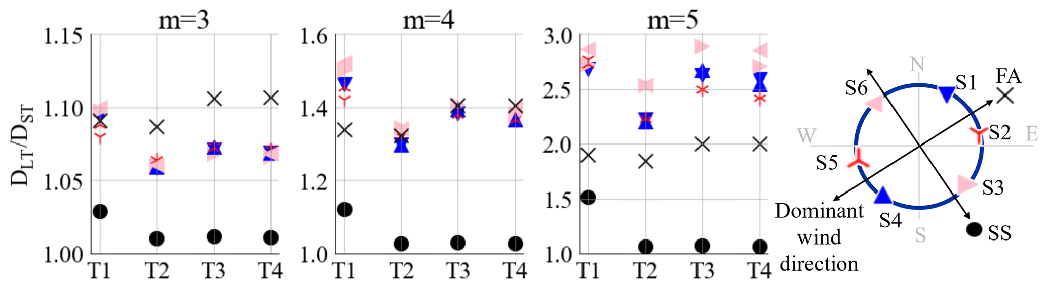
Figure 7 Average of the stabilized LFFD factors after 9 months for the six positions along the circumference and FA and SS, for T1 of Farm 1 and T2, T3, and T4 of Farm 2. Each box is for an SN curve slope.

If we take the average of the sensors for each turbine, the difference between turbines in the same farm is below 0.02, 0.1, and 0.3 for m=3, 4, and 5, respectively (refer to Appendix A). The wind and wave conditions for the three turbines in the same farm are quite similar. Therefore, the difference from one turbine to another might be explained by the different reactions of the turbine's structure to these loading conditions. T2 has the lowest LFFD factors because this turbine experienced more parked conditions compared with T3 and T4.

In parked conditions the importance of wave-induced loading increases, while the low-frequency wind loads are reduced significantly, ultimately reducing the LFFD damage. Moreover, the fatigue loading is larger in parked conditions; as a result, T2 has accumulated more base damage than T3 and T4. The higher base damage (without LFFD) and lower added LFFD damage will lead to a lower LFFD factor.

The FA LFFD factor is slightly higher than those for the sensors for m=3, but with the increase in m, sensors' LFFD factors overcome FA. That is because, with the increase in the SN slope, the added LFFD damage due to the wind direction grows. SS always has the lowest LFFD factors. The LFFD factors of FA and SS can be up to around 1.1, 1.4, and 2 and 1.03, 1.1, and 1.5 for m=3, 4, and 5, respectively.

Since Farms 1 and 2 significantly differ in design and natural frequencies, a comparative study helps to understand if and how these differences can affect the short- to long-term fatigue damage LFFD factor behavior and value. From Fig. 7, it seems that overall the low-frequency fatigue effect is different between the two farms, with higher LFFD factors for Farm 1 for all values of m. If we take the average LFFD factor of the sensors for each turbine, the difference between turbines in the two farms is below 0.05, 0.2, and 0.5 for m=3, 4, and 5, respectively (refer to Table A1). Conversely, T2, T3, and T4 are larger structures (the resonance frequency is lower and therefore closer to the wave frequency); therefore the damage is more affected by waves, and wave loading gives less low-frequency variation in damage.

For each SN slope, the variability of the LFFD factor is less between sensors compared with FA and SS. For sensors and SS, the shift in the turbine in a farm causes less change in the factor compared with the shift in the farm. While for FA, the shift in the farm yields a greater change in the factor compared with the change in the turbine in a farm.

As expected, opposite sensors show similar, if not precisely identical, LFFD factors due to the circular symmetry of the support structure. In all four turbines, the sensors perpendicular to the dominant wind (S3 and S6) have higher LFFD factors. Surprisingly, the sensors that are mostly affected by the thrust loading (S1–S4 and S2–S5 pairs) have lower LFFD factors. We observed that among the sensors normal and parallel to the dominant wind direction, the differences in base damage (T) are larger than the differences in the added LFFD damage. Therefore, the LFFD factor of sensors parallel to the wind is lower than the sensors normal to the wind.

4.3 Role of LFFDs with bilinear SN curves

In this study, until here we analyzed the effect of linear SN curves with slopes equal to m=3, 4, and 5 on the LFFD factor. These SN curves are mainly used to calculate the damage-equivalent moments (DEMs). But to calculate the fatigue damage of OWTs, bilinear SN curves are widely used. In Fig. 2, two commonly used bilinear curves from DNV (2019) are selected to study the change in the LFFD factor with the use of bilinear instead of linear SN curves. Both SN curves are partially at slopes m=3 and m=5 for large and small stress cycles, respectively. As a result, the bilinear SN curve will penalize large cycles, such as those caused by LFFDs, less than a single-sloped m=5 curve. A fundamental consideration is that for bilinear curves, the LFFD factor will be dependent on the stress ranges. Depending on whether the majority of stress cycles fall in the m=3 or m=5 region, it will result in a lower or higher LFFD factor, respectively. In Fig. 8, the LFFD factor of four turbines is analyzed after 1 year with the aforementioned bilinear SN curves. To investigate the role of the overall stress range, a stress concentration factor (SCF) is introduced in Eq. (8):

$$\begin{array}{}\text{(8)}& \mathrm{\Delta }{\mathit{\sigma }}_{\mathrm{SCF}}=\mathrm{SCF}\cdot \mathrm{\Delta }\mathit{\sigma }.\end{array}$$

Figure 8 Trend of LFFD factor versus SCF for all turbines for both DNV_D_A and DNV_D_CP.

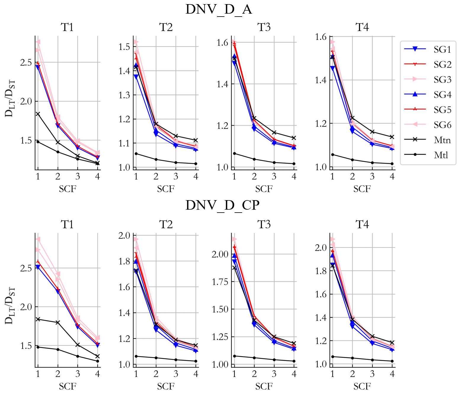
In Fig. 8, the SCF is varied from 1 to a maximum of 4, and LFFD factors are calculated for each value of the SCF. Note that the results hold for any (combined) multiplier on the stress ranges, e.g., a material factor (Natarajan, 2022). Figure 8 shows that as the SCF increases, the LFFD factor decreases. This is because the higher SCF shifts the fatigue spectra upwards towards a higher stress range, into the m=3 region of the bilinear SN curve, as a result pushing the LFFD factor closer to the LFFD factor of the linear SN curve with m=3. However, even with an SCF of 4, the LFFD factors of sensors and FA from the bilinear curves were not as low as those from the linear SN curve with m=3. On the other hand, the bilinear SN curve generally resulted in a lower LFFD factor compared with the linear SN curve with m=5, even when the SCF was 1. Due to the lower stress ranges, which are mostly affected by the m=5 region and do not reach the m=3 part of the bilinear curve at all, there is a significantly smaller difference between the linear and bilinear LFFD factors for the smallest turbine (T1) compared with other turbines. Thus, the fatigue spectrum continues to be in the m=5 region of the bilinear curve, even after applying an SCF of 4.

Furthermore, the LFFD factors from the SN curve with cathodic protection (DNV_D_CP) are higher than those from the SN curve in the air (DNV_D_A). This is because the transition of the DNV_D_CP curve to m=3 is at higher stress ranges, making the LFFD factors closer to the LFFD factors from the linear SN curve with m=5. An interesting point to note is the FA LFFD factor of T1 for DNV_D_CP, which from SCF = 1 to 2 does not have the same sudden drop compared with other cases. This is explained by the fact that the full fatigue spectrum remains in the m=5 region even with SCF = 2.

5 Conclusions

This study examined long-term OWT fatigue using 3 years of SHM data. We found that at least 1 year is needed to achieve a reliable LFFD factor. Our results are specific to the North Sea and are influenced by site-specific parameters, including weather conditions and structural dynamics. As a result, LFFD factors will vary (significantly) when considering different sites and turbines, and knowing the number of elements playing a role in this factor, we recommend quantifying it site specifically using in situ measurements. Our findings show that at the studied sites, the LFFD factor is the lowest for the SS direction and mainly the highest for fixed headings, an effect that strengthens for larger SN slopes. Considering the effect of gradual variabilities (LFFD) in the analysis can contribute significantly to damage – up to 65 % for an individual sensor and a Basquin slope of m=5.

Given that wind speed and direction interact to create low-frequency cycles, it usually takes more than a day for both variables to have a large impact simultaneously, which leads to a larger importance of weekly and monthly cycles in overall fatigue damage for individual headings compared with the FA and SS directions. The majority of the low-frequency cycles last less than a day, and the share of low-frequency cycles in the total damage increases for higher slopes in the SN curve. Fatigue analyses on the strain sensors showed that the heading has a secondary effect on the LFFD factor.

The LFFD factor calculated from one turbine can be roughly used for other turbines within the same farm. Also, LFFD factors for different wind farms with different support structure designs can vary with up to 50 % and 110 % for linear SN curves with m=5 and bilinear SN curves with $m=[\mathrm{3},\mathrm{5}]$, respectively. The bilinear curves cannot produce conclusions that are generalizable since the LFFD factor varies from spectrum to spectrum.

In future work, we plan to use the LFFD factors whenever the recovery of the low-frequency fatigue from cycle-count histograms cannot be directly applied, e.g., when only DELs are available (see Appendix C) or when we lose the time sequence in the data (like bootstrapping or binning the short-term damages). A further study on the quantification of LFFDs based on Supervisory Control and Data Acquisition (SCADA) will also be done for cases where no strain measurement is available.

Appendix A

Table A1 lists the observations of the converged LFFD factors after 9 months from Fig. 5a and for the three turbines of Farm 2. In addition, the values for m=3.5 and 4.5 are included. The highest LFFD factors for m=3, 4, and 5 are, as you can see, approximately 1.1, 1.5, and 2.9, respectively. And for m=3, 4, and 5, the maximum 2 SDs are roughly 0.02, 0.1, and 0.5, respectively.

Table A1 The converged LFFD factors for sensors, FA, and SS for all four turbines.

Appendix B

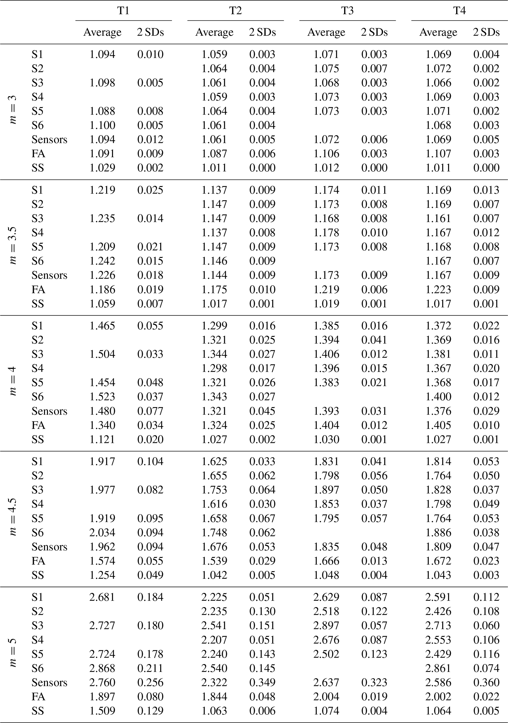
Figure B1 shows the share of low-frequency cycles with multiple aggregation window lengths. As shown, the shares of LFFD damages in the same farm are similar, except for the lower share of T2, since it was parked more. In general, the share of LFFD damages (except for SS) is almost similar for T1 and other turbines.

Figure B1 Share of low-frequency cycles with different cycle periods for turbines of Farm 2.

Appendix C

The damage-equivalent load (DEL) derived from a load time signal history for a chosen single-slope SN curve (typically m=3, 4, and 5 for steel) and an equivalent number of cycles (typically $N_{\mathrm{eq}}=\mathrm{1}\times {\mathrm{10}}^{\mathrm{7}}$) creates the same amount of fatigue damage as the Miner damage derived from the original load time signal on the same SN curve. The DEL is a direct quantification of fatigue loads derived from load measurement time series. The DEL from simulations is made during the design phase under the condition that the SN curve characteristics (m and N_eq) are the same. The DEL can be utilized as an alternative for damage because the Miner damage cannot be measured physically and requires a more refined selection of the SN curve. We use DELs with SN slopes of m=3, 4, and 5 in accordance with established practices (DNV, 2016). Considering the logarithmic distribution of damage, DEL is often employed in the design process of (offshore) wind turbines since it offers a linear scale for presenting damage. This choice ensures independence from the SN curve's intercept and improves readability.

In this appendix, we show how the short- to long-term fatigue damage LFFD factor could be applied to convert a short-term DEL into a long-term DEL. For the demonstration, we need the definitions of DEL (Natarajan, 2022) (or, more specifically, DES, as it is a damage-equivalent stress range), the SN curve in Basquin's law, and the Palmgren–Miner rule.

$$\begin{array}{}\text{(C1)}& {\displaystyle }& {\displaystyle }\mathrm{DES}={\left({\displaystyle \frac{\sum _{j=\mathrm{1}}^{N_{\mathrm{blocks}}}{n}_j(\mathrm{\Delta }\mathit{\sigma }{)}_j^m}{N_{\mathrm{eq}}}}\right)}^{\mathrm{1}/m}\text{(C2)}& {\displaystyle }& {\displaystyle }(\mathrm{\Delta }\mathit{\sigma }{)}^m=a/N\end{array}$$

By substituting Eq. (C2) into Eq. (C1), one retrieves the definition of DES concerning the Palmgren–Miner rule.

$$\begin{array}{}\text{(C3)}& {\mathrm{DES}}^m\cdot N_{\mathrm{eq}}=\sum _{j=\mathrm{1}}^{N_{\mathrm{blocks}}}{n}_j(\mathrm{\Delta }\mathit{\sigma }{)}_j^m=a\cdot \underset{\mathrm{PM}\mathrm{rule}}{\underbrace{\sum _{j=\mathrm{1}}^{N_{\mathrm{blocks}}}{n}_j/N_j}}\end{array}$$

Therefore,

$$\begin{array}{}\text{(C4)}& {\mathrm{DES}}^m\cdot N_{\mathrm{eq}}=a\cdot D.\end{array}$$

Applying the definition of the LFFD factor leads to

$$\begin{array}{}\text{(C5)}& \begin{array}{rl}{D}_{\mathrm{LT}}& ={\mathrm{DES}}_{\mathrm{LT}}^m\cdot {\displaystyle \frac{N_{\mathrm{eq}}}{a}}=D_{\mathrm{ST}}\cdot \mathrm{LFFD}\mathrm{\_}\mathrm{factor}\\ & =\left({\mathrm{DES}}_{\mathrm{ST}}^m\cdot {\displaystyle \frac{N_{\mathrm{eq}}}{a}}\right)\cdot \mathrm{LFFD}\mathrm{\_}\mathrm{factor},\end{array}\end{array}$$

from which the relation between DES_LT and DES_ST is straightforward:

$$\begin{array}{}\text{(C6)}& {\mathrm{DES}}_{\mathrm{LT}}={\mathrm{DES}}_{\mathrm{ST}}\cdot \mathrm{LFFD}\mathrm{\_}{\mathrm{factor}}^{\mathrm{1}/m}.\end{array}$$