the Creative Commons Attribution 4.0 License.
the Creative Commons Attribution 4.0 License.
 | 06 Mar 2023
On the laminar–turbulent transition mechanism on megawatt wind turbine blades operating in atmospheric flow
Brandon Arthur Lobo
Özge Sinem Özçakmak
Helge Aagaard Madsen
Alois Peter Schaffarczyk
Michael Breuer
Niels N. Sørensen
Among a few field experiments on wind turbines for analyzing laminar–turbulent boundary layer transition, the results obtained from the DAN-AERO and aerodynamic glove projects provide significant findings. The effect of inflow turbulence on boundary layer transition and the possible transition mechanisms on wind turbine blades are discussed and compared to CFD (computational fluid dynamics) simulations of increasing fidelity (Reynolds-averaged Navier–Stokes, RANS; unsteady Reynolds-averaged Navier–Stokes, URANS; and large-eddy simulations, LESs). From the experiments, it is found that the transition scenario changes even over a single revolution with bypass transition taking place under the influence of enhanced upstream turbulence, for example, such as that from wakes, while natural transition is observed in other instances under relatively low inflow turbulence conditions. This change from bypass to natural transition takes place at azimuthal angles directly outside the influence of the wake indicating a quick boundary layer recovery. The importance of a suitable choice of the amplification factor to be used within the eN method of transition detection is evident from both the RANS and URANS simulations. The URANS simulations which simultaneously check for natural and bypass transition match very well with the experiment. The LES predictions with anisotropic inflow turbulence show the shear-sheltering effect and a good agreement between the power spectral density plots from the experiment and simulation is found in case of bypass transition. A condition to easily distinguish the region of transition to turbulence based on the Reynolds shear stress is also observed. Overall, useful insights into the flow phenomena are obtained and a remarkably consistent set of conclusions can be drawn.
- Article
(14632 KB) - Full-text XML
- BibTeX
- EndNote


Wind turbines operate continuously in the atmospheric boundary layer and often under augmented inflow turbulence conditions such as in the wake of other wind turbines, on irregular terrains, in extreme weather conditions, and in wind shear. However, the airfoil sections used for the blade designs are tested in wind tunnel experiments that do not account for the unsteady inflow turbulence and the rotation of the rotor. This causes deviations in the aerodynamic performance of the wind turbine operating in atmospheric conditions from the predicted performance. A common procedure in blade design to account for the uncertain operating conditions on a rotor is to use an empirical blend of airfoil data based on natural transition and fully turbulent boundary layer flow. Moreover, the turbulent kinetic energy (TKE) spectrum in the free atmosphere is remarkably different from that typically generated in a wind tunnel. This was clearly identified in the DAN-AERO experiments (Madsen et al., 2010b) carried out in 2009, where the inflow to an airfoil section in the wind tunnel and on a 2.0 MW rotor was compared and characterized by the pressure fluctuations in the laminar boundary layer at the leading edge of the airfoil section. Much higher energy contents of the pressure fluctuations from the inflow were seen on the blade section on the rotor in a frequency interval up to about 300–500 Hz. Adding a turbulence grid in the wind tunnel decreased the difference somewhat but then caused the spectrum in the wind tunnel to exceed the rotor spectrum for frequencies above 500 Hz. In Schaffarczyk et al. (2017) it is reported that in the case of atmospheric flow, the TKE spectrum possesses a maximum at around 0.01 Hz followed by a decrease according to Kolmogorov's law, whereas in a wind tunnel experiment with a turbulence grid much more energy is distributed in the kHz range.
As a part of the MexNext project (Boorsma et al., 2018), transitional studies were carried out on a rotor model in a wind tunnel under varying operating conditions but in the absence of added inflow turbulence. An analysis of the experimental data showed that natural transition of the Tollmien–Schlichting (T–S) kind took place (Lobo et al., 2018). As a part of this project, the first comparisons between CFD (computational fluid dynamics) predictions using turbulence models including transition modeling and such an experiment was conducted by four groups, and a reasonable agreement with the transition location compared to the experimental data was found (Schaffarczyk et al., 2018). However, in the case of atmospheric inflow, different transition scenarios are expected. This depends on, for example, the length scales and turbulence intensity (T.I.) of the flow field. It is well known that for a T.I. in the order of 0.5 % to 1 % transition through T–S instabilities can be expected (Reshotko, 1976, 2001), while with a rise in T.I. bypass transition (Morkovin, 1969) occurs. Bypass transition is a broad term encompassing transition scenarios, where the initial growth is not described by the eigenmodes of the Orr–Sommerfeld equation. In such scenarios, transient growth is often observed, where decaying perturbations in terms of the eigenfunctions of the Orr–Sommerfeld equation undergo temporary amplifications on account of their non-orthogonality (Butler and Farrell, 1992; Reshotko, 2001). This can result in Klebanoff modes or streaks (Klebanoff et al., 1962) in the streamwise direction, which are regions of relatively high or low velocity relative to the mean flow. Such characteristics were observed in the measured surface pressure fluctuations in the DAN-AERO experiments (Madsen et al., 2010b).
This non-modal growth can be related to the free-stream disturbances through a mechanism known as shear sheltering (Hunt and Carruthers, 1990), which permits disturbances to penetrate up to a certain depth within the boundary layer. The penetration depth was found to depend on the frequency of the disturbance and the flow Reynolds number, with lower frequencies being able to penetrate deeper into the boundary layer (Jacobs and Durbin, 1998). Zaki (2013) illustrated the shear filtering effect with a model problem that used two scales: the lower frequency penetrated the boundary layer near the leading edge resulting in the generation of streaks as a boundary layer response. This is followed by their breakdown through a process known as the lift-up mechanism (Kline et al., 1967), where negative perturbation streaks rise within the boundary layer. The external high-frequency disturbances, which are limited in their penetration, provide excitation for the growth of an outer instability leading to turbulent breakdown of the streak.
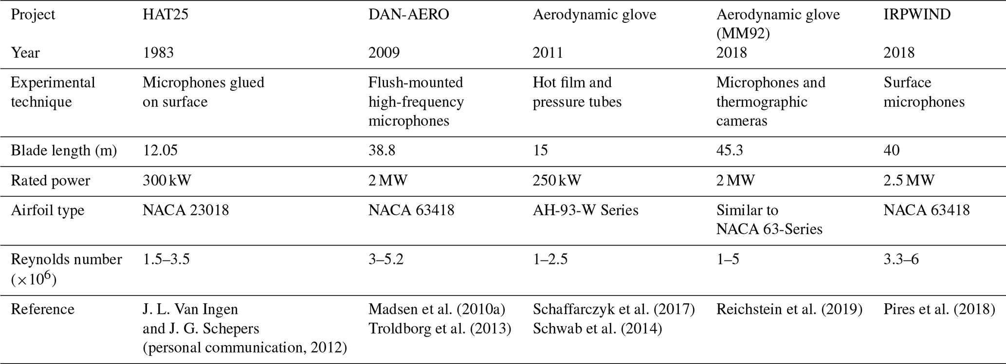
To better understand the transition phenomena on a wind turbine in the field, experimental data are necessary. A limited number of field experiments dedicated to laminar–turbulent boundary layer transition on wind turbine blades in atmospheric conditions are available as listed in Table 1. The analysis of the DAN-AERO and aerodynamic glove1 experiments release a significant amount of information on the transition mechanisms on wind turbine blades.
Madsen et al. (2010a)Schaffarczyk et al. (2017)Reichstein et al. (2019)Pires et al. (2018)Troldborg et al. (2013)Schwab et al. (2014)Table 1Field experiments on boundary layer transition on wind turbine blades (regenerated and extended from Özçakmak (2020)).
This paper focuses on the results from these experiments in comparison with numerical simulations with models of different fidelity. This study focuses on the impact of atmospheric turbulence on the boundary layer transition on wind turbines. It should be noted that direct comparisons were not always possible on account of the different parameters that were measured or on account of the limitations of the numerical techniques and/or resource limitations. However, in all cases, interesting findings related to transition on wind turbine blades are presented. First, the experimental findings from the DAN-AERO and aerodynamic glove projects focused on laminar–turbulent boundary layer transition are presented. This is followed by a brief summary of RANS (Reynolds-averaged Navier–Stokes) simulations for boundary layer transition that was conducted as a part of the IEA Wind Task 29 for the DAN-AERO blade. URANS (unsteady Reynolds-averaged Navier–Stokes) simulations based on the DTU (Technical University of Denmark) in-house CFD solver EllipSys3D (Sørensen, 1995; Michelsen, 1992, 1994) are then presented in comparison to the DAN-AERO experiments. Finally, LESs (large-eddy simulations) on a blade section corresponding to the aerodynamic glove experiments are discussed in detail. The LES predictions rely on the HSU (Helmut Schmidt University) in-house code ℒℰ𝒮𝒪𝒞𝒞 (Breuer, 1998, 2000, 2002, 2018) combined with the synthetic inflow generator by Klein et al. (2003). To conclude, general findings from these unique field experiments and simulations are summarized to shed light on different transition mechanisms and the effect of the atmospheric flow on the transition of the flow around wind turbine blades.
This section discusses the experimental findings from the projects DAN-AERO and aerodynamic glove on boundary layer transition analysis on wind turbines.
2.1 DAN-AERO
A significant part of the DAN-AERO project (Madsen et al., 2010a; Troldborg et al., 2013) was concentrated on the investigations of the laminar–turbulent boundary layer transition on an LM-38.8 blade of the 2 MW NM-80 rotor placed in a wind farm and on a 2D airfoil, which was a replica of this blade section. The blade section, which is 36.8 m from the hub, was equipped with pressure taps. As the frequency response of the pressure taps is low, the section was also equipped with high-frequency flush-mounted microphones for transition measurements. The details of the instrumentation and the sampling frequencies are described by Özçakmak et al. (2020). Detailed boundary layer transition analyses were performed in subsequent studies (Madsen et al., 2019; Özçakmak et al., 2019, 2020) by analyzing the DAN-AERO data further and conducting CFD simulations for the 2D and the full rotor flow.
2.1.1 Experimental findings from DAN-AERO
Boundary layer transition was detected based on the surface pressure fluctuations captured by the high-frequency microphones. Power spectral densities (PSDs) of these fluctuations are integrated with a frequency range from 2 to 7 kHz to calculate the root mean square (RMS) values. This was chosen according to a parametric study for various Reynolds numbers, where higher frequencies due to resonance in the tubing system caused by the pinhole placement of the microphones are excluded (Özçakmak et al., 2018). The lower frequencies are eliminated due to the possible effect of inflow turbulence or large eddies that would interfere with the spectra. On the condition that a certain threshold is exceeded, a sudden chordwise increase in RMS values indicates the transition location.
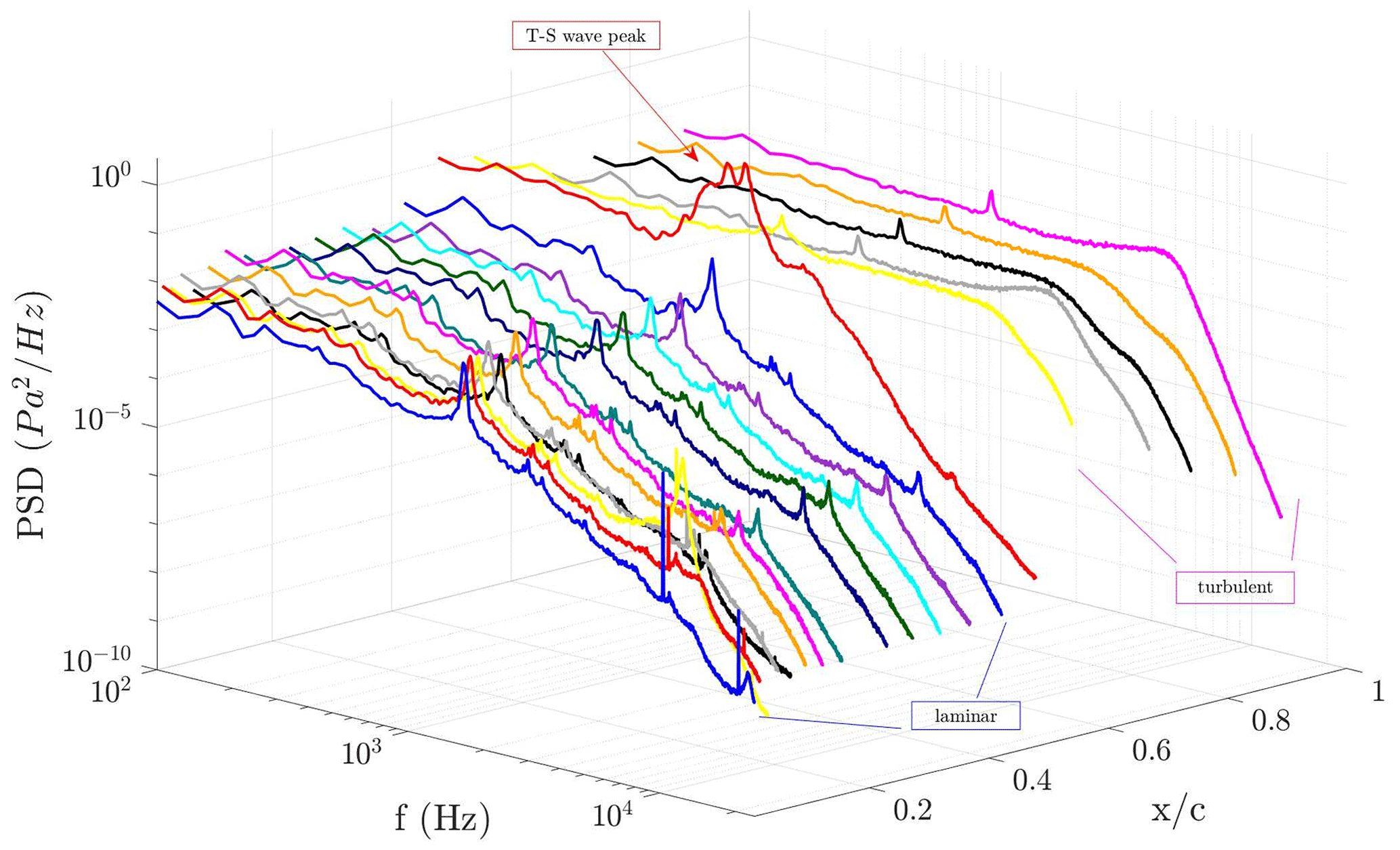
It is found that it is possible to determine the type of transition from the spectra. Different transition mechanisms were observed in the experiments. In the case of natural transition, the flow goes through a gradual process of three steps. In the receptivity step, initial disturbances occur in the boundary layer on account of external disturbances. Viscous instabilities such as Tollmien–Schlichting (T–S) waves are triggered inside the boundary layer. Then, these unstable waves go through the second step of linear instability through a linear amplification process (Arnal et al., 1998). In the third step, non-linear interactions in the form of secondary instabilities occur when the unstable wave amplitude grows and reaches a finite value (Reed and Saric, 1989). It is possible to follow T–S wave frequencies with a sufficient amount of microphones placed along the chord. Figure 1 shows the PSD vs. frequency f at different chordwise positions () on the pressure side of an airfoil model tested in a wind tunnel at , AOA = 0∘. This model is a replication of the LM-38.8 blade section (featuring a 18 % thick airfoil). Laminar spectra are observed at the chord positions until (red line), where lower energy at higher frequencies are found compared to turbulent spectra. The small peaks (around 1684 Hz) that are observed on the laminar spectra are due to the blade passing frequency of the fan in the wind tunnel (see Özçakmak et al., 2019). The microphone at this position shows transitional flow spectra with a T–S wave peak as indicated in the figure. Then the flow becomes turbulent downstream of (yellow line). Since transition does not take place at a point but is a process occurring over a certain distance, a higher resolution of the experimental instruments would show a longer chordwise process of natural transition. In the case of a higher resolution, it is possible to observe the mentioned peak growing before reaching a fully turbulent spectrum. It should be noted that the other peaks in the spectra are due to acoustic resonances in the wind tunnel.
As the analysis moves from the flow on a 2D airfoil to a full-scale wind turbine, inflow turbulence is found to be the predominant factor that influences the transition behavior as well as the angle of attack changes in a single revolution. Additionally, surface roughness has an important influence on the transition characteristics.
Since there was a lack of high-frequency inflow velocity fluctuation measurements in the field experiments, pressure fluctuations from the surface microphones in the laminar boundary layer close to the leading edge are used to analyze the inflow turbulence characteristics in detail (Madsen et al., 2019). Therefore, inflow turbulence is interpreted from a leading-edge microphone at % in the laminar boundary layer using pressure fluctuations as shown in Eq. (1), where Ps,p is the power spectral density of the microphone signal, σ is the standard deviation, and f1 and f2 are the integration frequency boundaries.
For the field experiments, a sketch for the wake-affected rotor area and the azimuthal notation is shown in Fig. 2. This notation will be used in the following figures.
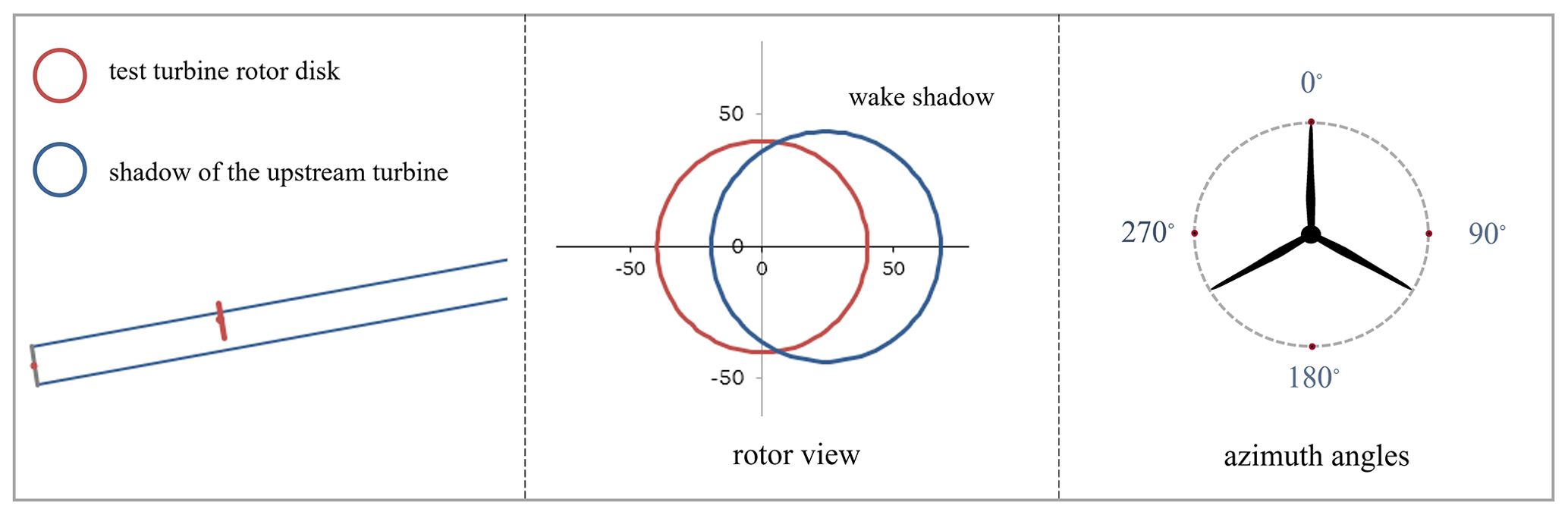
Figure 3 shows the PSD from this microphone for both wind tunnel and field experiments. It is obvious from the wind tunnel experiments that the pressure spectra from the clean tunnel and the tunnel with the turbulence grid represent the differences in the inflow conditions. Thus, this microphone can be used to demonstrate the inflow turbulence characteristics. It is seen that the tunnel with a grid has a higher amplitude of pressure fluctuations compared to the clean tunnel case. Two angles of attack are presented here which represent the effective range of angles seen in the field measurements.
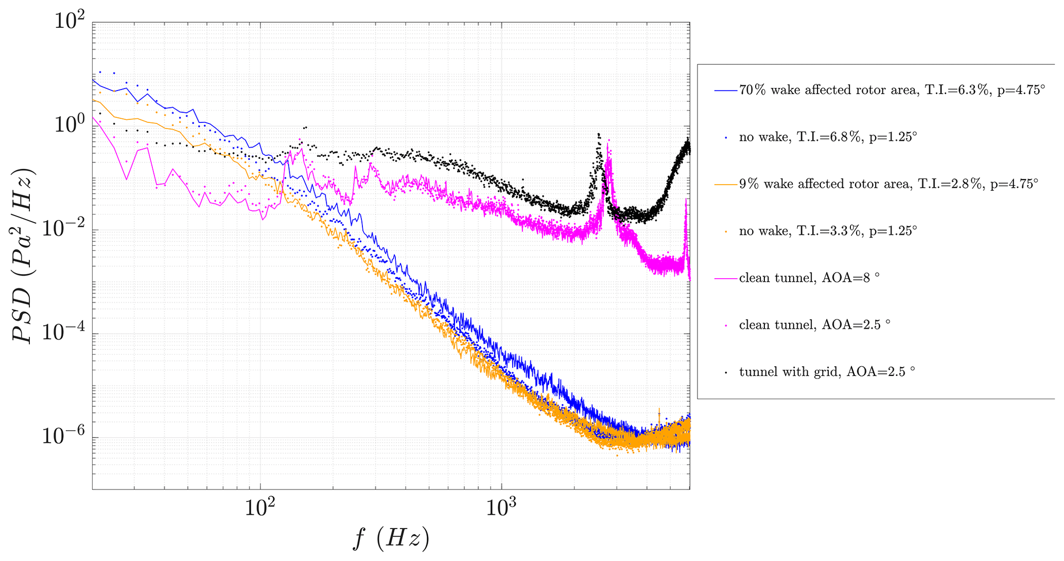
Figure 3Inflow spectra characterized by the pressure fluctuations in the laminar boundary layer for wind tunnel and field experiments obtained by a microphone placed at % on the pressure side.
As for the field experiments, the turbine is operated in two different pitch settings at 1.25 and 4.75∘, respectively. For both settings, a low and a high turbulence intensity value (calculated from the inflow velocity data obtained by the Pitot tube on the blade) are presented. Since the test turbine was placed in a wind farm at certain wind directions, it operates under a wake-affected inflow, mentioned as the percentage of the rotor disk area with wake-affected inflow (see Fig. 2). It is seen from the PSD data obtained in field experiments that as the pitch angle increases, the magnitude of the PSD also slightly increases (see dashed blue vs. solid blue line in Fig. 3). On the other hand, for the same pitch setting, increased inflow turbulence levels move the PSD magnitude to even higher values. This increase is mostly visible in the lower frequencies up to approximately 400 Hz. For the clean tunnel, the influence of the angle of attack is not as predominant as the influence of the inflow turbulence on the pressure side; on the other hand, its effect would be more prominent on the suction side for positive angles of attack. Furthermore, it is observed that the wind tunnel with a turbulence grid has more magnitude in spectra compared to the clean tunnel.
In a previous study (Madsen et al., 2019), it is found that integrating the spectra from 100 to 300 Hz (f1 and f2 in Eq. 1) for a high-frequency microphone placed in proximity to the leading edge, and inflow turbulence characteristics can be interpreted.
Figure 4 demonstrates a case where the inflow velocity is 6.3 m s−1 and T.I. is 6.3 %. The turbine has a pitch setting of 4.75∘, and it is operating in a wake resulting from an upstream turbine, where 69 % of the rotor area is affected. The various PSD lines are obtained from different time segments by a microphone placed at %. This microphone, at different times, due to the fact that the angle of attack and the inflow turbulence changes and operates under laminar, transitional, and turbulent flows. At the time of 2.5 s, it is under transitional flow, and at 4.1 and 8 s it shows laminar spectra. At 6.4 s it is operating under turbulent conditions.
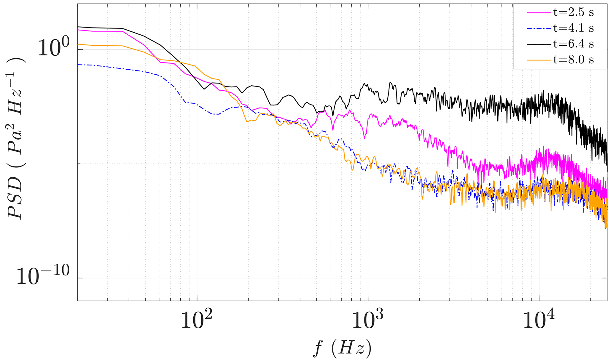
Figure 4Comparison of the PSD from different time indices for the same microphone placed at %.
This movement in transition locations is also shown in a spectrogram plot (Fig. 5) of the chordwise pressure levels, Lp (dB) in time for this case. Sound levels are calculated according to Eq. (2), where the reference pressure (Pref) is 20 µPa.
The sharp color changes mean there is a sudden increase in the standard deviations of the pressure fluctuations above a certain threshold, which indicates transition.

Figure 5Chordwise pressure levels (Lp) with a line of detected transition locations. The arrow indicates the time instances where the chordwise PSD values were plotted in Fig. 6.
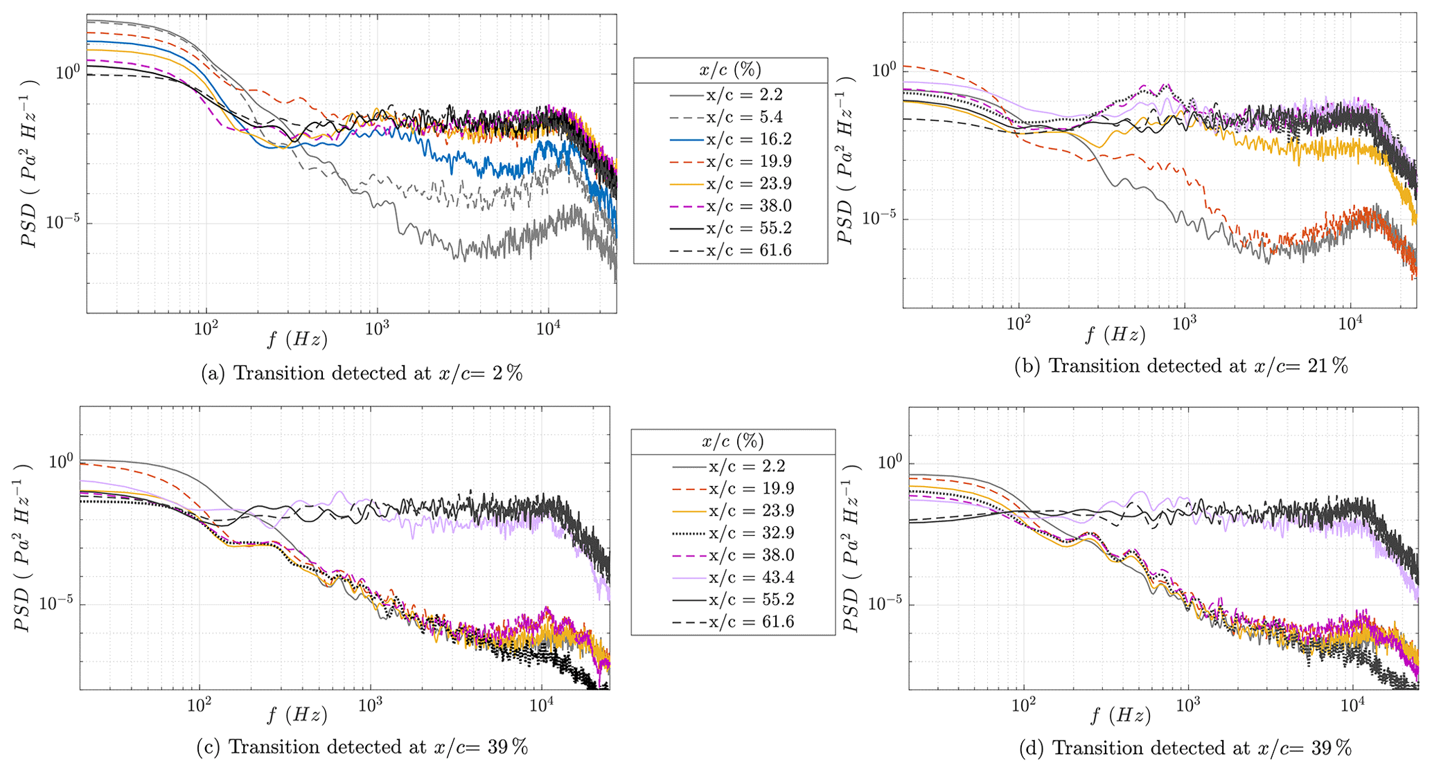
Figure 6PSD at various positions at different time indices (corresponding to the points a, b, c, d shown at Fig. 5) during a single revolution where the transition is detected at the chordwise location of (a) %, (b) %, and (c) %.
Both a change in the location of the transition due to the angle of attack changes and also due to inflow turbulence can be seen in a single revolution. The locations where the transition is detected at (denoted c and d) and (denoted b) are due to the angle of attack changes. However, the locations where the transition moves close to the leading edge are possibly due to the direct effect of inflow turbulence (bypass transition) (denoted a) in addition to the effect of the angle of attack changes.
For further analysis, the chordwise spectra of these time segments are analyzed and presented in Fig. 6. It can be seen from Fig. 6b that, when there is a natural transition, there is a growth of the T–S waves that occur as a peak in the spectra before the flow becomes turbulent as also demonstrated for the wind tunnel case in Fig. 1. The peak starts at % and it grows further downstream until a fully turbulent spectrum is observed. The weighted average of the T–S wave frequency is around 809 Hz. A peak that is slightly above the turbulent spectra is also visible for the case where the transition is found at % in Fig. 6c and d. However, at this location, the transition is possibly occurring on a small portion of the chord so that only one microphone was able to catch this peak. There is a more noticeable peak in case c than in case d, possibly because the c position is just the start of the change in the transition location from 21 % to 39 % (see also Fig. 6). At location d, the transition position is already established at 39 %. For the bypass transition case (Fig. 6a), it can be seen that the PSD magnitude is much higher in the lower frequency range up to approximately 400 Hz compared to the natural transition cases (b, c, and d). In this case, a T–S wave pocket growth is not observed that causes a peak in the spectra; instead, an increase in the high-frequency fluctuations of the spectra is found as the flow becomes turbulent. Moreover, all the microphones, even the ones in the laminar range, respond to this inflow turbulence also at high-frequency ranges.
2.2 Aerodynamic glove experiment
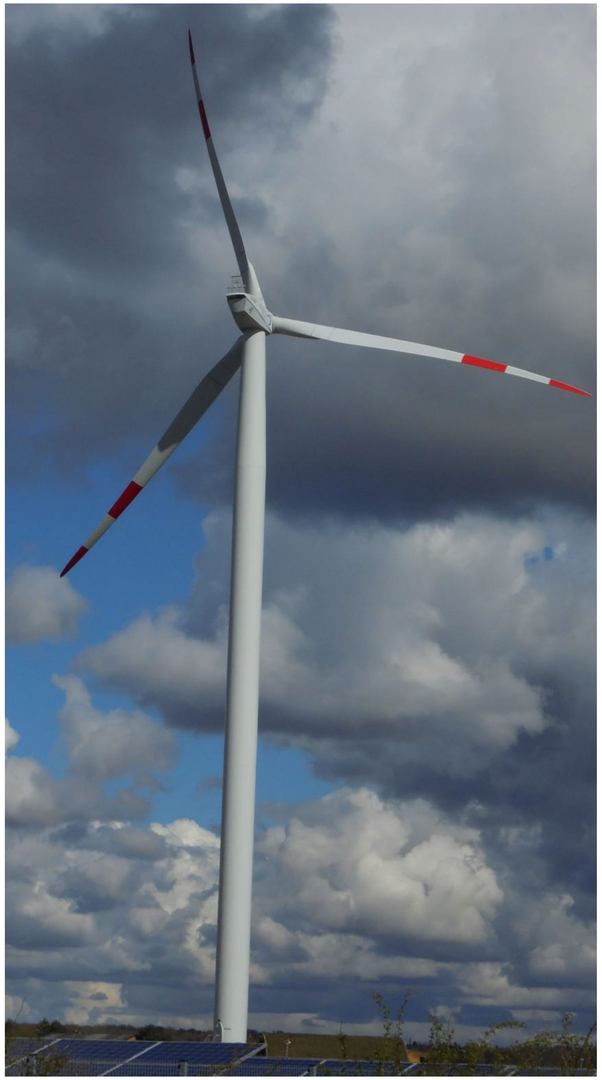
After preliminary investigations on a 15 m ENERCON E30 blade (Schaffarczyk et al., 2017), a similar measurement campaign was undertaken on a LM 43P blade mounted on the 2 MW Senvion (REpower) MM92 wind turbine (Reichstein et al., 2019) as seen in Fig. 7. Transition was intended to be detected by an array of microphones similar to the DANERO experiment discussed above but additionally enhanced by ground-based thermography carried out by two teams: DLR, Göttingen, and Deutsche Wind Guard Engineering (DWGE), Bremerhaven. In Dollinger et al. (2019), the potential for localizing transition on wind turbine rotor blades using thermographic techniques has already been proven but was not previously validated using simultaneous reference measurements.
The experiment consisted of different measuring techniques as highlighted above. An aerodynamic glove consisting of carbon fiber fabrics is laminated onto 20 mm thick foam plates which are aligned to the blade geometry to ensure the best fit possible. To determine the state of the flow, 48 microphones are used of which 43 are equally spaced on the suction side. The microphones are placed into the glove on a straight line with an inclination of 20∘ with respect to the chord to minimize the effect of upstream microphones. The microphone data were recorded at 25 kHz. Additional data such as pressure measurements, acceleration, temperature, and humidity were also measured as described in Reichstein et al. (2019). The thermographic measurements by DWGE used indium-antimonide (InSb) as the detector material and are sensitive in the mid-wave infrared band (between 2 and 5 µm), with the experiment being set up such that a spatial resolution of 11.2 mm is achieved with the instruments placed at a distance of 140 m from the wind turbine. The second setup provided by DLR is installed at a distance of about 80 to 85 m downstream of the wind turbine mast with an unobstructed view of the suction side of the aerodynamic glove. Here, mercury cadmium telluride (MCT) was used as the detector material and is sensitive in the long-wave infrared band (between 8 and 9.4 µm) and set up such that a resolution of 12 mm is achieved. More information on the setup and the coupling with telephoto lenses for improved spatial resolution and the post-processing procedure can be found in Reichstein et al. (2019).
2.2.1 Experimental findings from the aerodynamic glove project
The determination of transition using the microphone data was carried out using the process described in Troldborg et al. (2013), where the power spectral density of the pressure signal from the microphones is calculated. The calculated sound pressure level (SPL) in decibels (dB) with a time resolution of 12 Hz is then plotted using a color map. Figure 8 shows the temporal evolution of the SPL for both the start-up as well as periodic-state case together with the local radially outward-directed acceleration. As seen, the overall value of the SPL is higher in the periodic-state case, and a distinct region near the leading edge is recognized with lower SPL values, indicating laminar flow, while the rest of the suction side has higher SPL values, indicating turbulent flow. A periodic variation with transition moving closer to the leading edge is seen (light green compared to dark blue), matching the peaks in the acceleration when the blade is pointed downwards on account of acceleration due to gravity and centrifugal force being in the same direction. It is expected that higher inflow turbulence is experienced as the blade passes through the wind shadow of the tower.
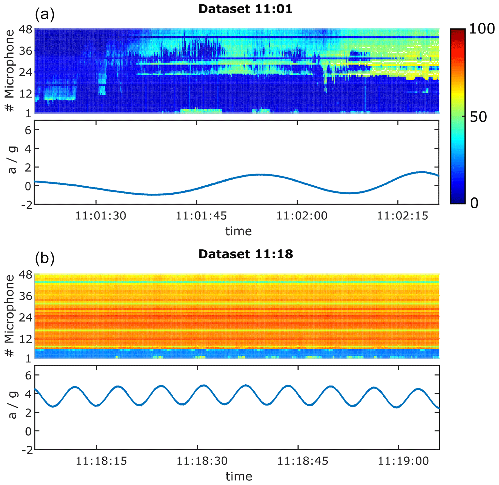
Figure 8Detection of the transition position. (a) Start up; (b) periodic state. Upper row: sound-pressure level (SPL) in decibels (dB). Color map: dark blue corresponds to 0 dB and red to 80 dB. Lower row: local acceleration.
Due to the very short time of data compilation (a few hours) and non-perfect surface preparation or a temporarily fouled surface by dust and/or insects, only a few data sets with large areas of assumed laminar boundary layer state could be recorded, see Figs. 9 and 10 for a typical example using thermographic imaging. The brighter areas in the picture indicate higher temperatures, which are interpreted as laminar flow. The magenta-colored parts show the pure blade and sky, respectively. DWGE uses the maximum temperature gradient to detect transition according to the algorithm by Dollinger et al. (2019). Locally at the location corresponding to the microphones, transition is detected at a chordwise location of . This result is consistent with that determined from the microphones with transition located at 0.26 at 11:15:32 (SCADA time). From the measurements by DLR, the midpoints of the transition zone from the instantaneous thermal images were found to be at a chordwise location of 0.370 (start-up) and 0.080 (steady operation at 9 RPM), which is very close to those detected by the microphone array at 0.34 and 0.070, respectively. Even though transition seems to be near the leading edge in the case of periodic-state operation on account of the imperfect surface, the main finding was equal accuracy of microphones and thermography with regard to the determination of transition location. Obviously, thermographic techniques do not provide as detailed information about the boundary layer as a microphone array, but they are evidently accurate enough for the detection of the transition location and already find practical uses, for example in leading edge corrosion detection.
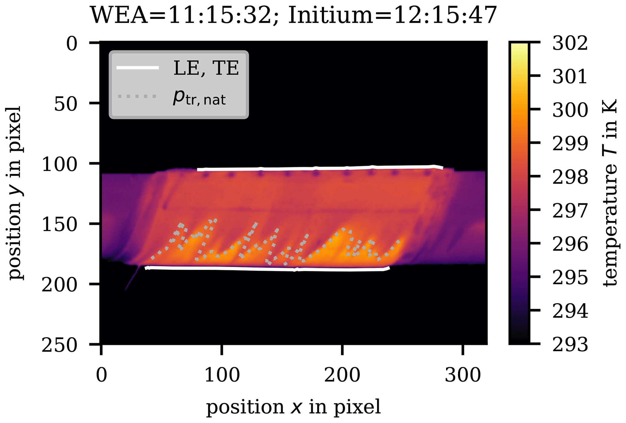
Figure 9Thermographic picture processed by DWGE. Leading edge (LE) bottom. Trailing edge (TE) further up. The dotted line indicates an automatically recognized transition by the post-processing system.
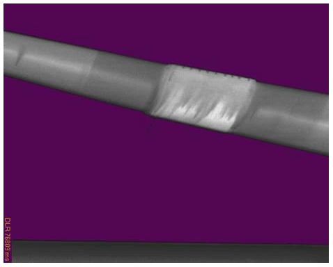
Figure 10Thermographic picture by DLR. Leading edge (LE) bottom. Light areas are assumed to be in a non-turbulent (laminar) state. Used by permission of DLR.
2.2.2 Transition from CFD calculations for the aerodynamic glove project
In parallel to the preparation of the experiment, 2D and 3D CFD simulations were carried out using DLR-FLOWer (FLOWer, 2008) and DLR-TAU (TAU, 2018), respectively. FLOWer was used in 2D mode to compute the friction coefficient distribution. Any conclusion about the location of transition relies on the underlying theoretical model. In the case of the glove experiments, variants of the eN method, assuming a Tollmien–Schlichting scenario to fully developed turbulence, were applied. Included here are some results from FLOWer and TAU as seen in Figs. 11 and 12, respectively. On comparison of the transition location during the start-up discussed above and as detected by the microphones and thermography, a good agreement with the prediction by FLOWer (Fig. 11) is found with transition detected at the location corresponding to the end of the laminar region (minimum cf) at and the beginning of the fully turbulent region at . 3D simulation results using TAU are shown in Fig. 12, with the flow regions highlighted in blue indicating laminar flow and red indicating turbulent flow. Transition is found to take place at 30 % chord at the mid-span. Due to the boundary effects, transition seems to move further upstream toward the edges. One of the difficulties in detecting transition using RANS CFD models is the justified choice of the N factor, often (esp. in wind tunnel measurements) related to the turbulence intensity: . Therefore, it would have been interesting to detect deviations from this specific scenario by comparing the expected transition location from 3D RANS calculations with that of the field experiment. However, as far as the observed locations of transition could be compared by CFD enhanced by transition prediction models, no such strong deviation could be found during the start-up phase. During the periodic-state operation on account of the non-smooth surface, transition moved far upstream, and no direct comparisons to CFD could be made.
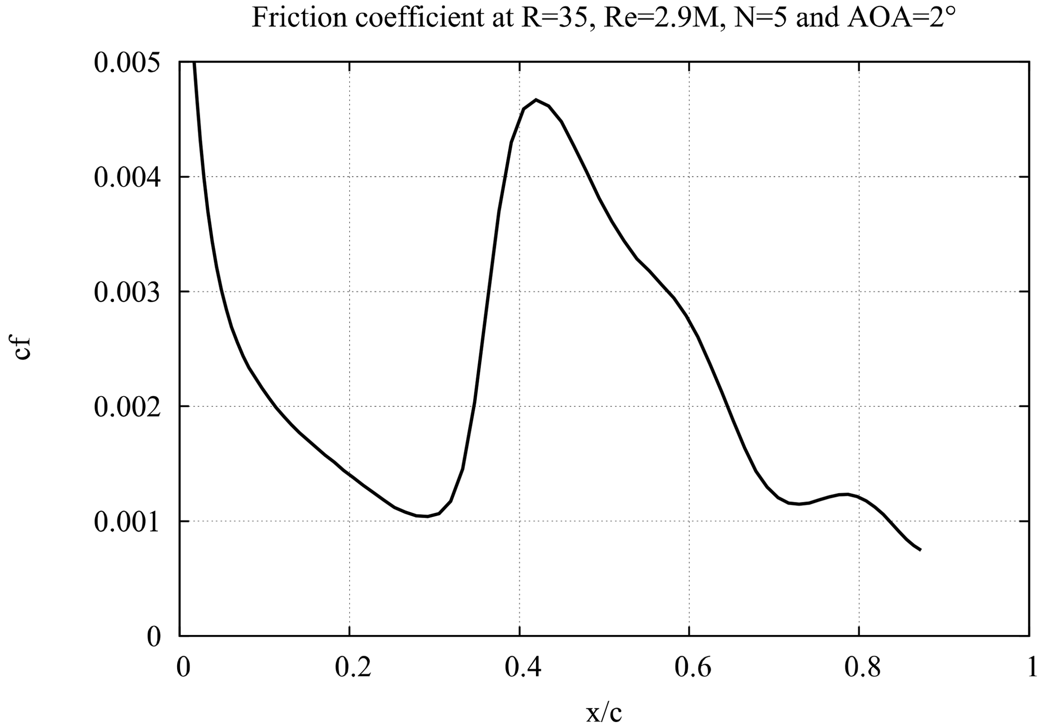
Figure 11Location of transition from wall shear stress by CFD code FLOWer. N = 5 corresponds to a T.I. of 0.3 %. The onset of transition may be located at , and the flow is fully turbulent at . The slope is at a maximum at
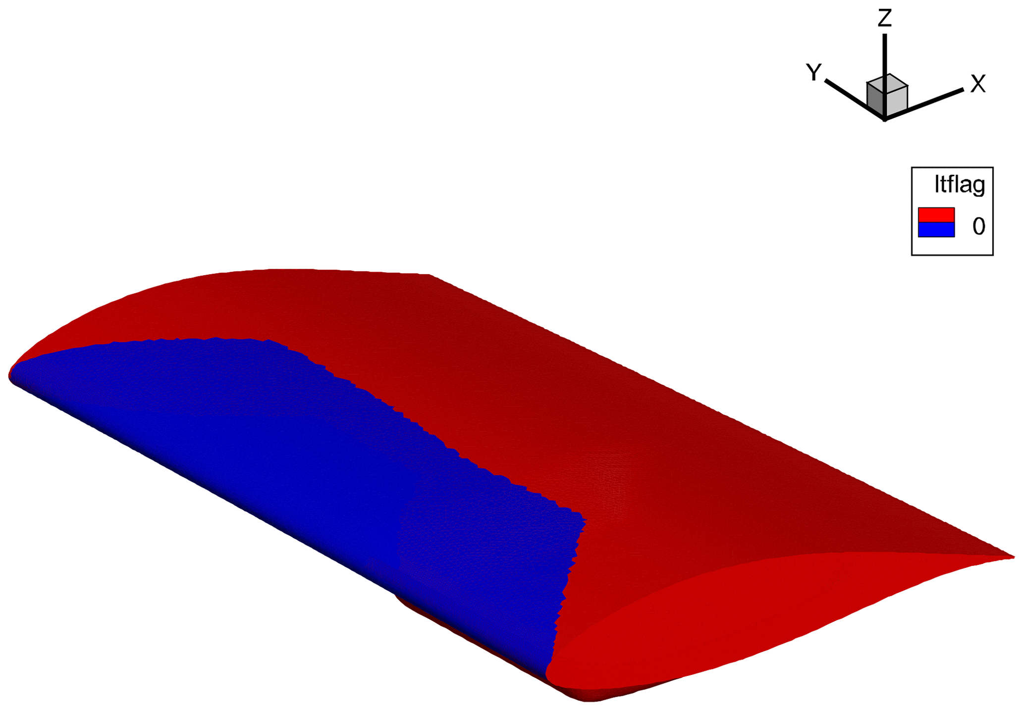
Figure 12Estimated flow state regions from 3D transitional CFD using the DLR -TAU code. Blue: laminar flow; red: fully turbulent flow. The transition location at the mid-span of the blade is located at 30 % chord.
To gain further insight into the transition phenomena on wind turbines, full rotor simulations and simulations across the wind turbine blade cross-sections have been conducted. This section discusses results from CFD investigations of increasing fidelity, with the goal of showcasing the capabilities and contributions of the different methods at their present state of the art. The following simulation methods will be discussed in the subsequent sub-sections:
-
RANS predictions with statistical turbulence models including transition modeling as described in more detail in Schaffarczyk et al. (2021),
-
unsteady Reynolds-averaged Navier–Stokes simulations as succeeding work for the model in the DAN-AERO project,
-
and large-eddy simulations as a follow-up of the aerodynamic glove project.
3.1 RANS – capabilities of modern codes
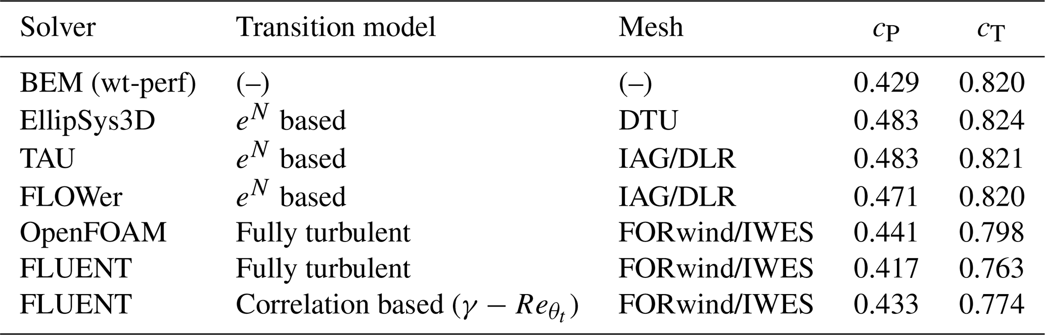
The analysis presented in this sub-section has been performed as a part of the IEA Task 29 under a sub-task on boundary layer transition (Schaffarczyk et al., 2021). It has been included here, in part, with the goal of presenting the capabilities of today's RANS codes with respect to wind turbine transition modeling. As a part of this IEA task, a limited number of teams performed 3D-CFD predictions including transitional modeling: The Technical University of Denmark (DTU) using EllipSys 3D, the Institute for Aerodynamics and Gas Dynamics in Stuttgart (IAG) using FLOWer, the Kiel University of Applied Sciences (KUAS) using Ansys FLUENT, the German Aerospace Center (DLR) using TAU, and the Fraunhofers Research Alliance for Wind Energy (IWES) using OpenFOAM. The simulations were carried out on the DAN-AERO NM80 wind turbine using the following parameters: rotor speed = 12.3 RPM (constant), wind speed = 6.1 m s−1, and pitch angle = 0.15∘ to feather (constant).
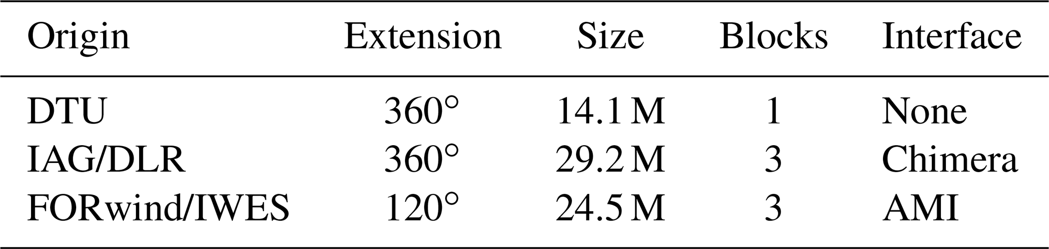
Presently, the methods typically used for the solution of RANS employs the SIMPLE algorithm for the pressure–velocity coupling together with a Gauss–Seidel algebraic multigrid method and a spatial discretization of second order (upwind). On account of the different requirements of the different codes, three different grids (see Table 2) were used by the teams for the purpose of the study. For example, at KUAS and using the commercial solver FLUENT, the original DTU mesh did not converge. This was probably due to the high aspect-ratio cells close to the wall of the blade. The IAG/DLR's mesh uses a Chimera technique with overlapping volumes. As a consequence, although a lot of effort was spent, it was not possible to convert these meshes for use with FLUENT. Therefore, the FORwind/IWES mesh, which used arbitrary mesh interfaces (AMI) that couple/interpolate different blocks at close but different 2D-interfaces, was employed.
Table 2Meshes prepared for RANS CFD models on the DAN-AERO NM80 blade (IEA Task 29).
As a turbulence model Fluent uses Menter's SST–k–ω (Menter, 1994) and to model laminar-to-turbulent transition uses Menter's Reϑ–γ transitional model (Menter et al., 2006) based on transport equations is applied. TAU uses a transition module that has implemented the eN method (Krimmelbein, 2009), which has been shown to work well for modeling natural transition (Özlem et al., 2017). Transition to turbulence in EllipSys3D is governed by the semi-empirical eN model (Drela and Giles, 1987). The transition model used by FLOWer is also based on the eN method, and OpenFOAM considers a fully turbulent case as described in Schaffarczyk et al. (2021).
Table 3 gives a short overview of the results for global values such as the thrust coefficient cT and pressure coefficient cP. Data were collected mainly from a presentation at the 2019 meeting of the IEA task 49 at NREL, Boulder, CO, USA. It is clearly seen that the overall cP and cT prediction with FLUENT is visibly (almost 10 %) smaller than the results of other codes (EllipSys3D, TAU, and FLOWer), with a deviation also seen in the results using OpenFOAM. A slight deviation in pitch (of about 0.4∘) was found but was discarded as the main reason for under-prediction because BEM (blade element momentum) calculations showed that a change of about 1 % would result on account of this. So, unfortunately, up to now it remains open what causes this rather big difference, but it is well known that the determination of the transition location, especially when using correlation-based transition models, depends heavily on the inflow conditions and the grid.
3.2 URANS full rotor simulations for DAN-AERO experiments
Unsteady Reynolds-averaged Navier–Stokes simulations are performed using the DTU in-house CFD solver EllipSys3D (Sørensen, 1995; Michelsen, 1992, 1994), using the exact model geometry from the DAN-AERO field experiments. The geometry and details of the mesh generation and simulation setup can be found in previous studies (Özçakmak et al., 2020, 2019).
A semi-empirical eN model (Drela and Giles, 1987) is used to model transition in EllipSys3D. In addition to the natural transition scenario, a bypass criterion can be used together with the eN model. In order to simulate high turbulence intensity cases, where bypass transition is observed, the empirical model of Suzen and Huang (2000) is used. In the code, criteria for both the natural and bypass transition are checked simultaneously. For the eN model different amplification ratios (N=0.15 to 7) and for the bypass model the relevant turbulence intensity values (calculated from the field experiments by the relative velocity on the blade) are introduced as an input.
Simulating all the inflow conditions with various atmospheric turbulence occurrences at once in an URANS setup and at the same time ensuring a detailed transition analysis is a highly complex problem. Therefore, all the occurrences are simulated in different simulation setups which includes the free-stream velocity range from 5 to 8.5 m s−1 (measured by the meteorological mast) and turbulence intensity values from 2.8 % to 6.8 %. A mesh is generated for the two different pitch angle (1.25 and 4.75∘) settings.
Figure 13 shows the intermittency values at the blade section y=36.8 m (relative radial position of 0.92) from the hub obtained from the full rotor simulations for a free-stream velocity w of 6.3 m s−1 and the pitch setting of p=4.75∘. The intermittency factor γ in the transition model governs the transition to turbulence by controlling the effective viscosity. The intermittency value γ of 1 represents turbulent flow, and the value of 0 represents laminar flow. The transition regions on the upper and lower surfaces of the blade section can be visualized in this way. Detailed information on the intermittency factor and its formulation in the transition model can be found in a previous publication by Özçakmak et al. (2020).
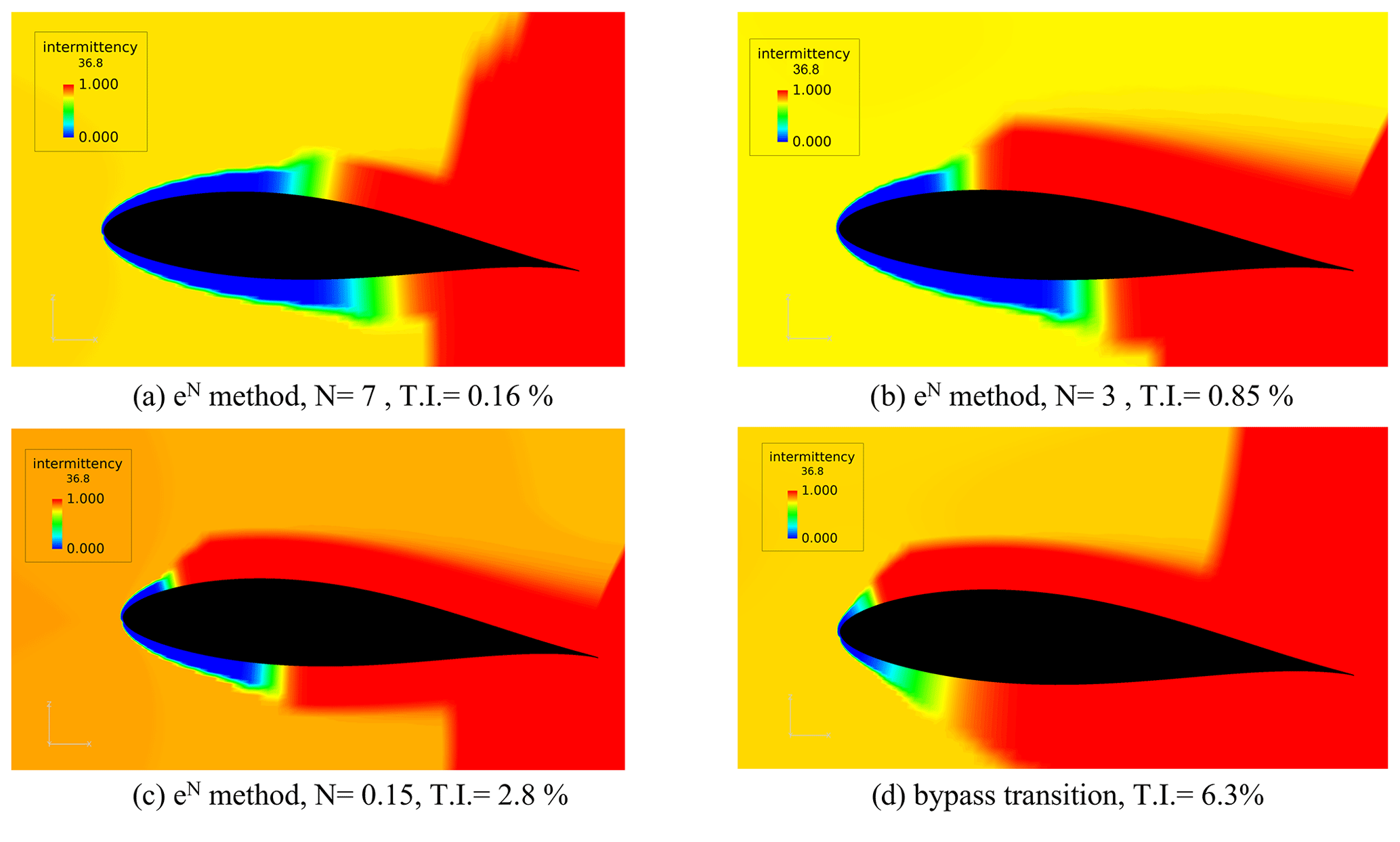
Figure 13Intermittency contours for the case at w=6.3 m s−1 and p=4.75∘ for the blade section at 36.8 m from the hub. The blade section results are obtained from the EllipSys3D URANS full rotor simulations.
All the visualizations and post-processing is performed using the FieldView software (FieldView, 2017). The four cases presented here are separate simulations, where the eN natural transition model is used for various N numbers of 7, 3, and 0.15 as shown in Fig. 13a–c, respectively. Moreover, Fig. 13d shows the results for the bypass transition model, where the turbulence intensity value is set to 6.3 %. The transition point moves upstream towards the leading edge as the amplification ratio is reduced (i.e., higher turbulence intensity values as shown by the Mack, 1977 relation: ).
In addition to the above simulations, a significant number of full rotor simulations were conducted with different transition models (eN and bypass transition) and inputs for the free-stream velocity, pitch setting, and inflow turbulence levels. During the post-processing, data from the section of one of the blades, which was instrumented with high-frequency microphones in the field experiments, are analyzed. The effective angle of attack in the simulations is calculated by the annular averaging of the axial velocity method in order to compare the results with the field experiments. The details of this method and how it is implemented can be found in previous studies (Hansen et al., 1997; Özçakmak, 2020).
An example case for a free-stream velocity of 6.3 m s−1 and T.I. = 6.3 % inflow conditions, where the turbine operates under the effect of a wake of an upstream turbine (69 % wake-affected rotor area) is shown in Fig. 14. Several simulations were performed since during a single revolution the angle, inflow velocity, and turbulence that the blades go through changes.
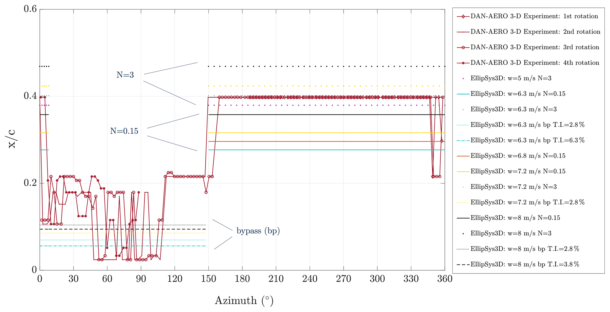
Figure 14Experimentally detected transition locations as a function of the azimuthal angle for the case at w=6.3 m s−1, %, and p=4.75∘ showing four revolutions. The EllipSys3D simulation results are labeled by the colors for various free-stream velocities, i.e., black: w=8 m s−1, yellow: w=7.2 m s−1, orange: w=6.8 m s−1, turquoise: w=6.3 m s−1, and purple: w=5 m s−1 (N=0.15, N=3, and N=7 correspond to T.I. values of 2.8 %, 0.85 %, and 0.16 %, respectively).
It is seen that at the azimuthal angles where the wake-affected inflow is present on the blade section, the simulation results obtained with the bypass transition model agree with the experimental results. Moreover, the natural transition zones show agreement with the semi-empirical eN method with N=3 for exactly the same free-stream velocity of 6.3 m s−1 as in the experiments. The selected case is operating in low-shear conditions. The angle of attack changes from 4 to 8∘, and the relative velocity on the blade changes from 62.5 to 66 m s−1, showing the same trend with azimuth angle as the transition position in Fig. 14. Furthermore, the inflow turbulence signals detected from a leading-edge microphone show higher values (100–115 dB) between 0 to 150∘ azimuth, and it decrease to a range of 85–105 dB between 150 to 350∘ azimuth, showing an opposite response than the other parameters with azimuth angle. The regions where the transition point is detected around 20 % of the chord are possibly due to the decreasing angle of attack on the pressure side. On the other hand, the regions where transition is close to the leading edge, as also predicted by bypass transition URANS simulations, are the direct effect of the inflow turbulence in addition to the effect of the decreasing angle of attack.
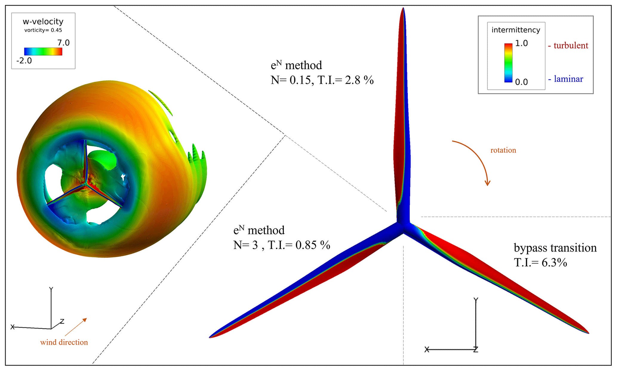
Figure 15EllipSys3D-vorticity iso-surfaces colored by the w velocity (wind direction) component (on the left) and intermittency γ contours on the pressure side obtained for three different inflow turbulence levels with natural and bypass transition models, shown in the same figure for representing the change of the transition line location throughout a single revolution (on the right) (w=6.3 m s−1).
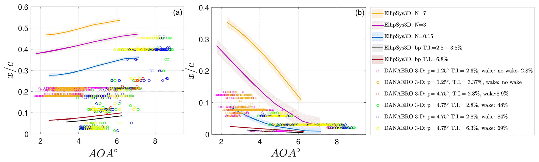
Figure 16Detected transition locations from the EllipSys3D computations and the DAN-AERO field experiments for the pressure (a) and suction (b) sides, regrouped and regenerated from Özçakmak et al. (2020).
Vorticity contours colored by the w-velocity component (free-stream velocity direction) obtained from the EllipSys3D full rotor simulations are shown in Fig. 15 (left) for w=6.3 m s−1, eN transition method with N=3 (T.I. = 0.85 %). It is seen from the iso-surfaces of the vorticity that the simulations are approximately axisymmetric. Furthermore, the intermittency contours on the blade for a case at w=6.3 m s−1 are presented in Fig. 15 (right). Each blade location represents different inflow conditions. When the blade is at the top position (azimuth angle of 0∘), and when at 225∘, the blade is operating out of the wake. Therefore, transition line results obtained from eN method (N=0.15 and N=3, respectively) are shown for those cases. Moreover, for the blade passing through 135∘ azimuthal position, the transition line calculated from the bypass transition model (T.I. = 6.3 %) is presented as it is operating under the wake of an upstream turbine at this position. All the results are gathered in a single rotor image, and in this way the changes in the transition line during a single revolution due to the changes in the angle of attack and the inflow turbulence are visualized (Fig. 15, right).
Analysis of several measurements from different days with various inflow velocities and turbulence conditions as well as two different pitch settings are collected in a single figure (Fig. 16) together with the EllipSys3D simulation results. The angle of attack values are derived from the force measurements in the DAN-AERO field experiments by obtaining a correlation between the normal force and angle of attack using the aero-elastic model of NM80 wind turbine using existing polars by HAWC2 (Larsen and Hansen, 2007) simulations based on blade element momentum theory. Detected transition locations from the high-frequency microphones are presented in this figure and grouped according to the pitch angle and wake-affected inflow conditions. The EllipSys3D results with different transition models and inputs are also presented for both pressure (Fig. 16, left) and suction sides (Fig. 16, right).
It is seen from the pressure side that within a single revolution, if the inflow wake-affected rotor area is large, then the change in the transition location is scattered along 44 % of the chord on the pressure side. On the contrary, in the low angle of attack region, when the wake-affected rotor area is small, the variation of the transition location along the chord during a single revolution drops to 5 %. The variation of the transition location during a single revolution is represented by separate EllipSys3D simulations conducted at various inflow conditions. EllipSys3D results for various amplification ratios can cover the range of the transition locations detected from the experiments. The experiments show an earlier transition compared to simulations for natural transition on the pressure side at low angle of attack values. For higher angles of attack, on the other hand, the location of numerical transition fits the results where there is natural transition. For the bypass transition case, EllipSys3D results are within the range of the experiments. It is seen that both natural and bypass-type transition mechanisms can occur in a single revolution of the turbine. Looking at the experimental results for a pitch angle of 4.75∘, for the same turbulence intensity value of 2.8 %, as the wake-affected rotor area increases from 9 % to 48 % (red dots to green dots), it is seen that the transition position starts to scatter more around the chord and bypass transition cases are observed for positions very close to the leading edge. Another comparison can be done between a low T.I. of 2.8 % value and a high wake case (blue dots) and high T.I. case of 6.8 % with similar wake conditions. A shift in the transition graph is observable through lower angles of attack, meaning earlier transition is observed at a certain angle of attack moving from blue to yellow dots, i.e., from the low to the high T.I. case.
It is relatively hard to comment on the suction side as the detected transition positions from the experiments are in very close proximity to the leading edge (varying from 1 % to 13 %). Moreover, some surface bumps that are visible from the pressure tap measurements could have played a role in changing the transition location on the suction side. However, it is still possible to see a good agreement between the simulations and the experiments.
3.3 Large-eddy simulations on an airfoil corresponding to the aerodynamic glove experiment
As a follow-up to the aerodynamic glove experiment on the Senvion (REpower) MM92 wind turbine (Reichstein et al., 2019), wall-resolved large-eddy simulations (LESs) are carried out to provide more insight into the transition phenomena that occur at Reynolds numbers in the order of a million under free-stream turbulence. The simulations are, however, carried out on a non-rotating section of the blade and at a reduced Reynolds number of one million. The profile considered corresponds to the section of the LM 43P blade at a radius of 35 m and a relative thickness of 20 %. The simulations focus on a fixed angle of attack of α=4∘ which lies within the range measured during the experiment. The Reynolds number of Re=106 is based on the chord length c and the free-stream velocity u. A parameter study with varying inflow turbulence intensities (T.I.s) is carried out as indicated in Table 4. All units with respect to the LES predictions are non-dimensionalized using the chord length and the inflow velocity. It must be noted that the inflow turbulence used does not consider blade rotation, nor are the length scales similar to the experiment on account of the large domain that would be necessary to accommodate these large structures, which is computationally unfeasible. For the same reason, the Reynolds number is reduced but on a similar order of magnitude. The goal of the LES analysis is to study the possible transition mechanisms that could take place at such Reynolds numbers in the presence of broad-band free-stream turbulence on a typical wind turbine airfoil, which can be thought of as a simulated wind tunnel experiment including lower frequencies that are typically not achieved in a wind tunnel when using active grids (Schaffarczyk et al., 2017).
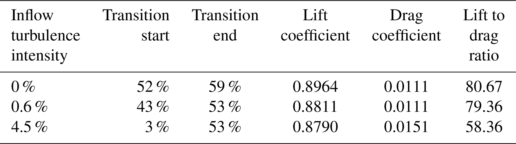
Table 4Flow configurations and observed transition locations using wall-resolved LES.
For the LES, the filtered three-dimensional, time-dependent Navier–Stokes equations for an incompressible fluid are solved based on a finite-volume method on block-structured grids, which is second-order accurate in space and time (Breuer, 1998, 2000, 2002). A blended scheme is used in space which is a combination of a standard central difference scheme (95 %) and a standard upwind scheme (5 %), whereas the time marching within the predictor–corrector method uses a low-storage Runge–Kutta scheme. In the present study, the widely used dynamic version of the classical Smagorinsky (1963) model is applied which was introduced by Germano et al. (1991) and Lilly (1992). The subgrid-scale stress tensor mimics the influence of the non-resolved small-scale structures on the resolved large eddies. A C-type grid with the angle of attack already included in the base mesh is used. The grid extends eight chord lengths upstream of the airfoil and 15 chord lengths downstream of the trailing edge avoiding the influence of the outflow boundary condition on the flow around the airfoil. This is a standard domain size, which is sufficient for LES as also seen in, for example, Gao et al. (2019) and Solís-Gallego et al. (2020). A suitable choice for the spanwise extension is critical for such geometrically two-dimensional airfoils. A width of is chosen for the present Reynolds number, which is sufficient as discussed in Lobo et al. (2022). The non-dimensionalized grid dimensions satisfy the typical requirements for a wall-resolved LES as outlined by Piomelli and Chasnov (1996) and Asada and Kawai (2018), details can once again be found in Lobo et al. (2022).
The generated inflow turbulence is anisotropic in nature and follows the Kaimal spectrum (Kaimal, 1973). The input parameters such as the relationship between the standard deviations in the three principle directions and length scales used for the generation of the inflow turbulence are based on those suggested by the IEC-61400-1 standard. According to this IEC standard, for hub heights greater than 60 m the relative length scale is Λ1=42 m. This is far too large for a computationally expensive LES, and therefore they need to be scaled down to maintain the anisotropic nature such that the eddies have a similar form but not the same absolute size. Since the spanwise extension of the domain is the limiting dimension (0.06 chord lengths), the length scales are chosen based on this parameter. The chosen length scales in the longitudinal, lateral, and vertical directions are 0.211, 0.07, and 0.017 dimensionless units, respectively.
The inflow turbulence for the simulations is generated by a synthetic turbulence inflow generator (STIG) based on the digital filter method proposed by Klein et al. (2003) and improved for computational efficiency by Kempf et al. (2012). The presently applied STIG only allows the definition of one length scale per direction. However, this disadvantage is compensated by superimposing the solutions of different length scales given by the maximal length scale divided by the factor 2n (n=1–5). The generated turbulence (see Fig. 17a) is then inserted by a source-term formulation (Schmidt and Breuer, 2017) into the domain close to the region of interest to prevent numerical damping due to the coarse grid resolution far away from the airfoil. This implementation has been thoroughly discussed in previous publications (Schmidt and Breuer, 2017; Breuer, 2018; De Nayer et al., 2018). Here, the inflow turbulence is inserted one chord length upstream of the airfoil. The resulting turbulence decay is minimal as can be seen in Fig. 17b. The decay of the free-stream turbulence defined as is plotted using the averaged normal Reynolds stresses in the three principle directions (i.e., etc.) at the end of the simulation period. Here, U denotes the mean inflow velocity. The slight rise seen at about close to the injection plane is due to the insertion of turbulence based on a Gaussian bell-shaped distribution around the inflow plane. The required inflow turbulence is achieved slightly downstream of this plane. The rise near the nose of the airfoil located at is due to the influence of the airfoil.
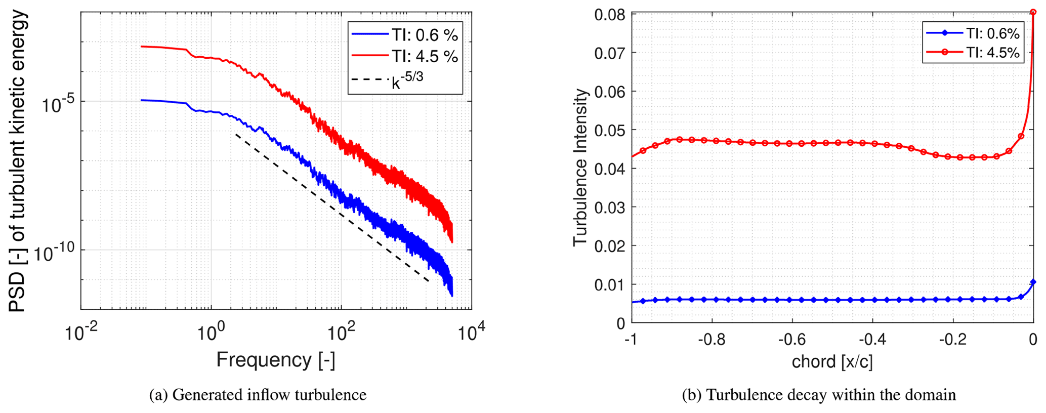
Figure 17Generated inflow turbulence and its decay within the domain along a line corresponding to the x axis.
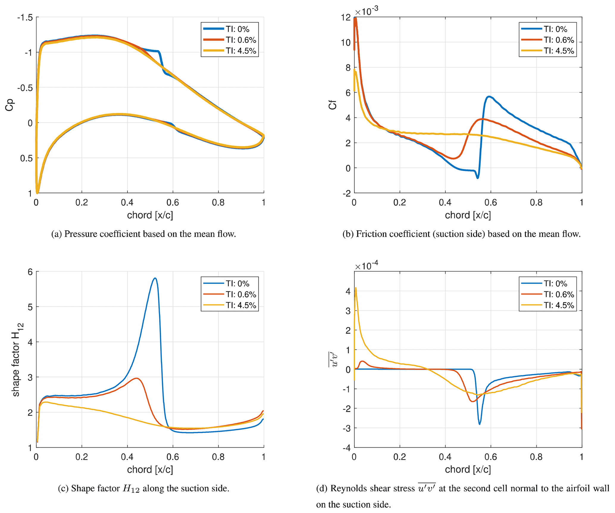
Figure 18Distribution of the aerodynamic properties of the airfoil from the LES (geometry corresponds to the LM 43P blade at a radius of 35 m from the hub) at a Reynolds number of 106 and α=4∘.
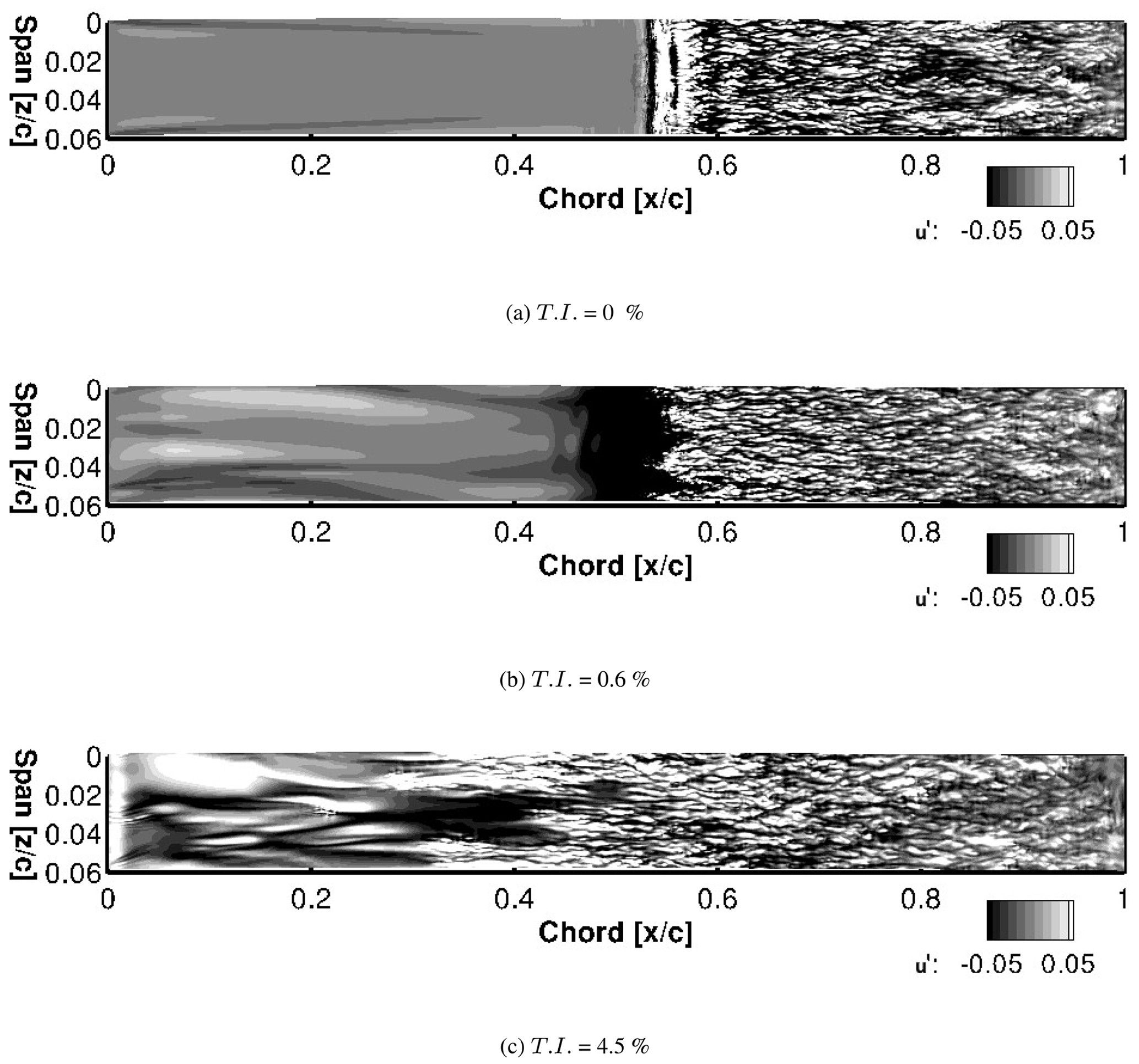
Figure 19Snapshots of the instantaneous streamwise velocity disturbance u′ for the visualization of boundary layer streaks. Slices are taken at a wall-normal height corresponding to the displacement thickness at 0.5 % chord.
At inflow turbulence of 0 % an obvious plateauing of the pressure coefficient is seen in Fig. 18a, indicating the presence of a laminar separation bubble between 50 % and 55 % chord. This is more apparent by the negative cf values in Fig. 18b. Here, transition to turbulence is clearly taking place between 52 % and 59 % chord as indicated by the sharp drop and then rise in cf before its eventual reduction, indicating a fully turbulent flow. The shape factor which is the ratio of the displacement thickness to the momentum thickness as seen in Fig. 18c is also helpful in distinguishing between the laminar and turbulent flow. The laminar, transitional, and turbulent regimes for the T.I. = 0 % case are quite evident with the drop in H12 between 52 % and 60 % chord, indicating transitional flow. This drop is due to the increase of the momentum thickness caused by shear, indicating an increased momentum exchange that takes place during transition. This increase in momentum exchange is clearly seen in Fig. 18d, where the Reynolds shear stress at the second cell in the wall-normal direction on the suction side is depicted. At an inflow T.I. of 0 % the Reynolds shear stress is zero along the suction side until a sharp rise of the magnitude is seen beginning at 52 % chord. A peak is found at 55 % chord, and finally, the magnitude reduces to a lower slope at approximately 60 % chord. This transitional region between 52 % and 60 % chord is in good agreement with that indicated by the shape factor. The peak at 55 % chord corresponds in this case to the reattachment point but is also a good indication of what will further be referred to as the peak transition to turbulence location. This can be visualized in Fig. 19a, where the instantaneous streamwise velocity disturbance u′ at a height corresponding to the displacement thickness at 0.5 % chord is shown. Here at 56 % chord, it is clearly visible that the flow has turned turbulent. Upstream of this position at 52 % chord, the location indicated above as the beginning of the transitional region also clearly shows a spanwise roll of the Kelvin–Helmholtz type, further showing that it is possible to distinguish the laminar and turbulent regions from the plots shown in Fig. 18.
With an increase in inflow turbulence to 0.6 % there is no more an indication of separation in the mean flow, neither in the cp nor in the cf plot. From the plot of the friction coefficient (Fig. 18b) a clear distinction between laminar, transitional, and turbulent flow regime is still evident with a laminar region up to approximately 43 % chord. Downstream of this position the flow is transitional between 43 % and 56 % chord, indicated by the rise in cf. Finally, the flow is found to be fully turbulent at 56 % chord. Transition to turbulence therefore moves upstream in the presence of added inflow turbulence. From the plot of the shape factor (Fig. 18c) a clear transitional region is once again visible, and it is interesting to note that the flow has a similar value of the shape factor when fully turbulent at around 58 % chord onward as that seen at 60 % chord with T.I. = 0 %.

Figure 20Distribution of the Reynolds shear stress in the wall-normal direction at selected chord locations.
For the cases with added inflow turbulence, the plot of the Reynolds shear stress (Fig. 18d) is a good indicator of the receptivity of the boundary layer to external disturbances, again due to the fact that this factor indicates momentum exchange. At T.I. = 0.6 % a small peak is seen at 4 % chord extending up to about 10 % chord, with a small but noticeable increase even up to 20 % chord. This case shows the shear-sheltering phenomenon (Hunt and Carruthers, 1990), wherein lower frequencies of the external disturbances (or inflow turbulence) have the capability of penetrating deeper into the boundary layer compared to higher frequencies. Moreover, the leading edge, having the thinnest boundary layer, allows for penetration of a higher range of inflow disturbances (Jacobs and Durbin, 1998). This is a fact clearly indicated by the rise of the Reynolds shear stress near the leading edge with a reduction as the flow moves downstream, showing a reduced interaction between the external flow and the boundary layer. Boundary layer streaks or Klebanoff modes (Klebanoff et al., 1962) are produced as a response of the boundary layer on account of the penetration of external disturbances. It is remarkable that even a low T.I. of 0.6 % results in the formation of boundary layer streaks as seen in Fig. 19b. They are visible as elongated dark (slower than the mean flow) and light (faster than the mean flow) longitudinal regions of the flow. Just as in the case without added inflow turbulence, for the case with a T.I. = 0.6 % the largest peak in the magnitude of the Reynolds shear stress at 53 % chord is the location at which the flow turns turbulent. This can further be confirmed by the plots of as seen in Fig. 20b where the profile begins to show the typical turbulent characteristics of a sharp peak near the wall followed by a region where there is an obvious change in the slope. The difference between 50 % and 53 % chord is obvious. Similar plots are also seen at a T.I. = 0 % (Fig. 20a) where the double peak typical for the turbulent region is first seen at 59 % chord. This matches the expected chord location from the friction coefficient and shape factor estimates.
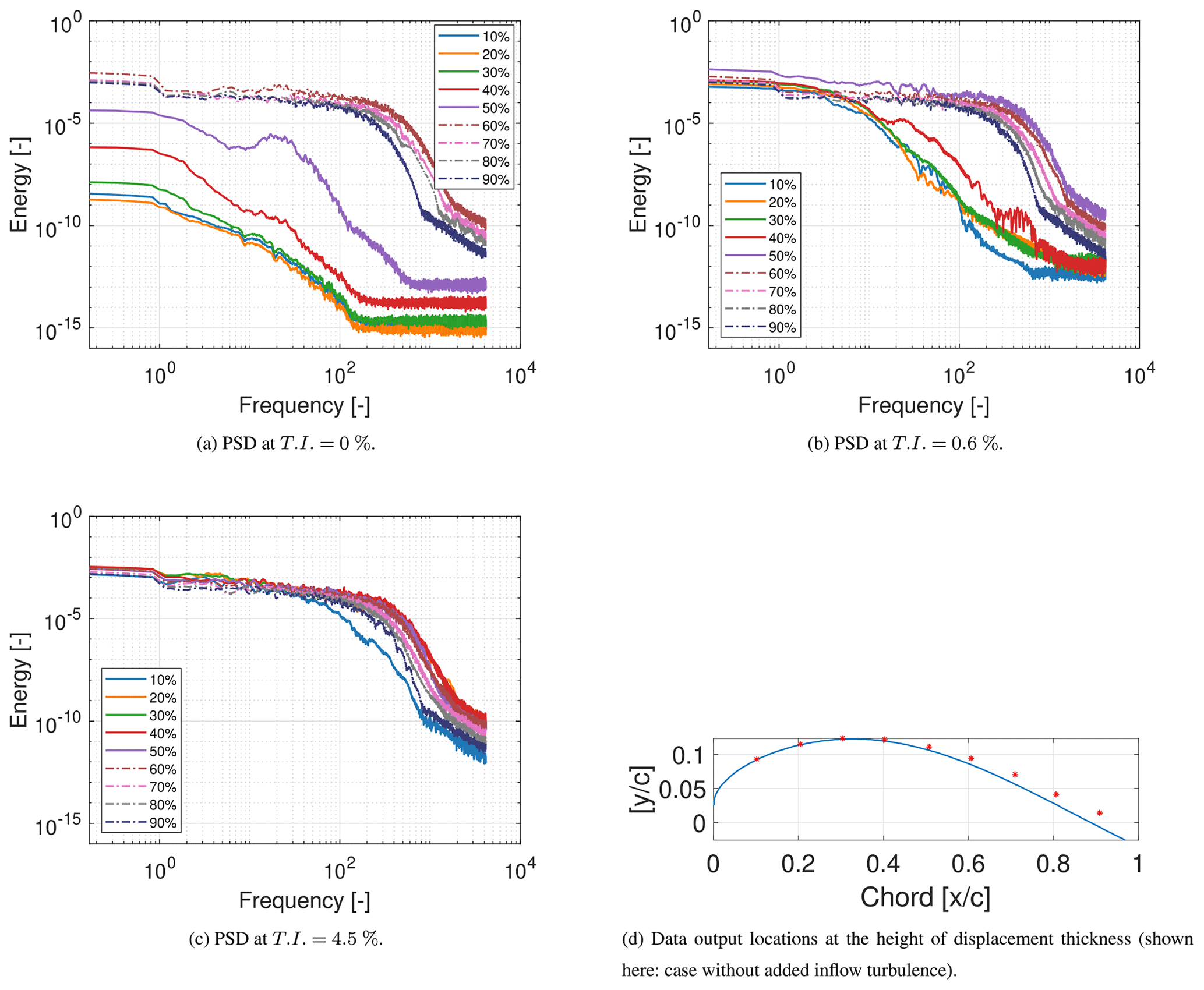
Figure 21Power spectral density of the turbulent kinetic energy at different T.I.s determined at the height of the displacement thickness in the mid-span at every 10 % chord.
On further increasing the inflow turbulence to 4.5 %, the cp curve (Fig. 18a) between 40 % and 50 % chord somewhat flattens in comparison to the case with an inflow T.I. of 0.6 %; i.e., the slight bump around the region where an inflectional instability was observed is not present anymore. Here, turbulent bursts of the varicose kind (Vaughan and Zaki, 2011) are also seen. Overall, especially on the suction side in the laminar region, up to approximately 50 % chord a further decrease in the suction-side pressure coefficient is seen, which results in a reduction of the overall lift with increasing inflow turbulence. Distinguishing between laminar, transitional, and turbulent flow, in this case, is not as easy as compared to the cases with lower T.I. discussed above. An increase in cf indicating transitional flow is not apparent in Fig. 18b as in the previous two cases. However, a relatively sharp drop is seen at approximately 50 % chord, indicating a change in the flow characteristics, probably a sign of turbulent flow. Using the plot of the shape factor (Fig. 18c) as an indication, the extent of the turbulent regime is quite similar to that at T.I. = 0.6 %, with the flow having similar characteristics beyond 56 % chord. There is once again no evidence suggesting a clear separation between the laminar and transitional zone. The flow seems to be already transitional near the leading edge at approximately 3 % chord. On investigating the Reynolds shear stress at different chord locations depicted in Fig. 20c, a turbulent profile with a peak close to the wall and an obvious change in slope as discussed in the previous two cases is first seen at 53 % chord. This coincides quite well with the location of the peak in seen in Fig. 18d. Thus, once again this peak can be used to detect the point at which the flow turns turbulent. Furthermore, a similar trend in is seen where the greatest exchange of momentum is towards the leading edge and the penetration of disturbances as indicated by the exchange of momentum decreases along the chord.
For a further investigation on the mode and process of transition and the influence of the inflow turbulence on the boundary layer receptivity, it is helpful to analyze the power spectral densities (PSDs) along the chord for the different cases under consideration. Figure 21 shows the PSD plots of the turbulent kinetic energy computed using a Hann windowing function on the data collected at a height corresponding to the boundary layer displacement thickness and at every 10 % chord. Data were collected at a dimensionless frequency of 8.3 k covering 6 dimensionless time units. Figure 21d indicates the regions where these quantities are evaluated.
At an inflow turbulence intensity of 0 %, a clear increase in energy is seen at 40 % chord with the separation bubble showing a sharp increase in energy at a frequency corresponding to 10 dimensionless units at 50 % chord. The highest energy in the spectra is then found at 60 % chord, with a decrease as one moves downstream. The region where the flow first turns fully turbulent is expected to have the highest turbulent kinetic energy (Özçakmak et al., 2019). At a T.I. of 0.6 % it is quite evident that the energy at 10 % chord is approximately a factor of 5 higher than in the absence of inflow turbulence. At 40 % chord there is a large increase in energy, indicating that the flow is transitional, and at 50 % chord the flow is turning turbulent as discussed earlier. Once again, this is the chord location with the highest energy, with a reduction seen as the flow proceeds downstream. It must be pointed out that there is a small peak at 10 dimensionless units which corresponds to the peak seen at T.I. = 0 %. This is on account of an inflectional instability.
On further increasing the inflow turbulence to 4.5 % it is nearly impossible to distinguish laminar and turbulent regimes. However, at 10 % chord the energy content is obviously lower than at the other chord locations but evidently higher than in the previous cases. This is due to the fact that the higher frequencies also have higher energy compared to the previous case, thereby allowing higher frequencies to penetrate deeper into the boundary layer. Furthermore, 40 % and 50 % chord have a similar and the highest energy, indicating that this is the location around which the flow turns fully turbulent. This is in agreement with the discussion above.
To optimize the aerodynamic design of wind turbine blades, it is essential that the transition process under varying conditions in the free atmosphere is better understood, thereby paving the way for the creation or improvement of existing transition models. Precise prediction of the transition location will lead to the design of more efficient blades and avoid the present design procedure where an empirical-based blend of airfoil data based on full turbulent and free transition simulations is used. For wind turbines in atmospheric flow and in the presence of inflow turbulence, especially in the wake of an upstream wind turbine, bypass transition is found to play an important role. The present study analyzes the transition on the LM-38.8 blade of the 2MW NM-80 rotor from the DAN-AERO experiment (Madsen et al., 2010b) and the LM 43P blade of the Senvion (formerly REpower) MM92 wind turbine corresponding to the aerodynamic glove experiment (Reichstein et al., 2019). Corresponding to these experiments, unsteady Reynolds-averaged Navier–Stokes (URANS) simulations and wall-resolved large-eddy simulations (LESs) are respectively carried out. Furthermore, an overview on the present capabilities of Reynolds-averaged Navier–Stokes (RANS) methods, which are computationally the cheapest, are presented with respect to wind turbine transition prediction thus showcasing the capabilities of computational fluid dynamics (RANS, URANS, and LES) at different levels of fidelity.
4.1 Experiments
-
From the experiments it is clear that even on turbines operating in the free atmosphere, laminar regions can be present, and this can be detected from microphone arrays and thermographic imaging techniques.
-
In case of bypass transition, inflow turbulence is found to be a predominant factor together with changes in the angle of attack during the revolution. The role of surface roughness cannot be ruled out or quantified.
-
The DAN-AERO experiment shows that the transition scenario changes even over the course of a single revolution due to the changing characteristics of the upstream flow field (change in angle of attack, shear, and upstream wake conditions). In this particular study, natural transition was found to dominate when the turbine operated outside the influence of an upstream wake, whereas in the presence of a wake, bypass transition was observed. Furthermore, the boundary layer recovery is evidently quite quick, with natural transition taking place at azimuthal angles directly outside the influence of the wake. The transition locations are detected by integrating the spectra in the range of 2–7 kHz and determining the highest derivative of this integration above a threshold. It is also observed that the type of transition can be estimated by the power spectral behavior from the amplification of the spectral energy around particular frequencies.
-
A high-frequency microphone placed at the laminar boundary layer region close to the leading edge and integrated over a low-frequency range (100–300 Hz) provides information about the inflow turbulence level, and this can be linked to the transition behavior. In the case of natural transition, three stages, namely receptivity, linear amplification, and non-linear interactions (secondary instabilities), could be visualized through power spectral density plots of the fluctuating pressure field. For high levels of the spectrum, the bypass transition is observed moving the transition point close to the leading edge.
-
With respect to the aerodynamic glove experiment, short experiment times and a non-perfect surface have led to only a few data sets with large areas of the laminar region. However, it can be concluded that at least the same accuracy of microphones and the two thermographic techniques with respect to the transition location are found.
4.2 3D-RANS with transition modeling
-
Deviations between the transition locations were found for the different codes tested, with the transition being detected between 20 % and 40 % chord on the suction side for the test case discussed. Transitional models showed larger deviations in the power coefficient when compared to the fully turbulent models, which showed a much smaller deviation of .
4.3 URANS
-
On separately calculating and analyzing various configurations of URANS simulations by using the DTU in-house CFD solver EllipSys3D, which simultaneously checks for natural and bypass transition, it is shown that there is good agreement between simulations and experiments with natural transition in the absence of an upstream wake and bypass transition in the presence of a wake.
-
High turbulence levels seem to trigger bypass transition in the boundary layer in addition to its effect on the effective angle of attack. The chordwise location of the bypass transition detected from the simulations is within the range of the experiment.
-
With respect to natural transition and on the pressure side, earlier transition was observed in the experiments when compared to the simulations at lower angles of attack, whereas at higher angles of attack the location of the numerical transition between the simulations and experiment tend to agree. It is relatively harder to make similar arguments on the suction side as the detected transition location from the experiments are in close proximity to the leading edge (between 1 % and 13 % chord). Surface bumps visible from the pressure tap measurements could have also played a role in transition. However, it is still possible to see a good agreement between experiments and simulations.
-
Similar to the 3D-RANS simulations, a justified choice of the amplification factor (N) is difficult to choose without experimental data to compare with. In this case an N factor between 0.15 and 3 provides reasonable results.
4.4 LES
-
The wall-resolved LES is successful in resolving various transition scenarios without any additional input such as an amplification factor N, nor does it depend on an intermittency factor as in the case of bypass transition using URANS methods.
-
At low inflow turbulence intensities it is quite easy to distinguish between laminar, transitional, and turbulent regimes from either the friction coefficient or the shape factor. With increased inflow turbulence, however, the flow seems to be transitional from close to the leading edge, and fixing a point where the flow turns turbulent is not as easy. Nevertheless, this is possible from the Reynolds shear stress distribution close to the wall, with the flow turning fully turbulent at the most negative values of due to the highest exchange of momentum at this point on account of transition.
-
The shear-sheltering effect is also evident based on the Reynolds shear stress distribution, with disturbances penetrating into the boundary layer over a larger chord length when the inflow turbulence is increased due to the augmented energy of the flow.
-
The power spectral density plots of the turbulent kinetic energy at the height of the displacement thickness are quite useful in determining the transition scenario and are comparable to those from the DAN-AERO experiment, with a clear growth of disturbances in the case of natural transition and higher energy in the low-frequency spectra in case of bypass transition. The PSD plots can also be used to determine the location of transition provided that a sufficient number of data points are recorded along the chord. The highest energy on the PSD of the TKE coincide with the transition location. The same is also seen in the wind tunnel study on the model blade section from the DAN-AERO experiment. This once again can be attributed to the highest exchange of momentum and thus fluctuations within this region.
-
The increase in energy in the lower frequency range with increasing inflow turbulence is comprehensible. The penetration of these low-frequency disturbances gives rise to boundary layer streaks which can also be visualized. With increasing inflow turbulence the number of streaks and their intensity increases. The spanwise wavelength does not seem to be influenced by the turbulence intensity alone and most likely depends on the length scales of the external disturbances.
-
In summary, LES enhanced by artificial anisotropic turbulent inflow mimicking flow conditions of the free atmosphere even at high Reynolds numbers ≥106 is possible and feasible with present-day high-performance computing technology at least for research purposes, even though it is still out of scope for industrial purposes.
In this study, a variety of experimental as well as numerical investigations have been carried out to understand the transition behavior on wind turbine blades. Overall, from the experiments and simulations, it is found that the laminar to turbulent transition and the different scenarios through which it takes place can be detected through experiments and predicted with reasonable accuracy through simulations. It is seen that the high-fidelity simulations are more reliable and provide data that can be used to better understand the underlying physics of the different transition phenomena. The transition scenario on a wind turbine blade is shown to change even within a single revolution with bypass transition taking place under enhanced upstream turbulence, such as the wake induced by an upstream wind turbine. Such an observation of bypass transition on account of the formation of streaks through the redistribution of momentum by the lift-up mechanism has also been observed through large-eddy simulations under increased inflow turbulence. In the DAN-AERO experiment, it was also found that the change from bypass to natural transition occurs at azimuthal angles outside the wake, indicating a quick boundary layer recovery. Simulating the location of transition by RANS and URANS methods required a suitable choice of the amplification factor to be used with the eN method, which then results in a good match between simulations and experiments. The LES predictions highlight the shear sheltering effect in the presence of inflow turbulence and display a similar spectrum of the power spectral density to that of the experiments in the case of bypass transition. Furthermore, the profile of the Reynolds stress, as determined from LES, can be used to identify the location where the flow turns fully turbulent. On the other hand, the traditional method of distinguishing this location based on the shape factor plot or from the spectra of the PSD is not so trivial for high inflow turbulence levels. Even though LES provides more comprehensive information for transition prediction, in the case of design computations it is computationally prohibitive for full-rotor simulations. Therefore, it must be emphasized that, for the foreseeable future, the industry will continue to rely on RANS/URANS methods along with eN and correlation-based methods for transition prediction.
In light of these results, more dedicated experiments measuring the transition process on blade sections in atmospheric flow are needed, e.g., quantifying the impact of the inflow turbulence intensity with high-frequency instruments. Additionally, high-fidelity LES predictions should be improved for simulating more complex inflow that represents experimental cases. These efforts would provide further useful insights into the transitional flow phenomena and advance our understanding of the fundamental transition mechanisms on wind turbine blades.
The codes used for the simulations presented here are the intellectual property of the authors or the university they are associated with. In case of interest, please contact the authors.
Interested parties can contact the corresponding author to discuss data accessibility.
APS, BAL, OSO, NNS, and HM participated in the IEA Task 29. HM was the project coordinator of the DAN-AERO experiments; OSO conducted the data analysis for boundary layer transition and interpreted the DAN-AERO results combining it with theory. NNS provided ideas, concept, and guidance for the URANS simulations; OSO performed the URANS CFD simulations and post-processed and presented the results. APS was involved in the aerodynamic glove experiment. BAL performed the LES simulations and its analysis under the guidance of MB (providing additionally the LES and STIG codes) and APS. BAL, OSO, and APS wrote the draft paper, and MB, HM, and NNS reviewed and edited the paper.
The contact author has declared that none of the authors has any competing interests.
Publisher's note: Copernicus Publications remains neutral with regard to jurisdictional claims in published maps and institutional affiliations.
RANS and LES computations by members of KUAS were performed with resources provided by the North-German Supercomputing Alliance (HLRN). Special thanks from KUAS go to Galih Bangga (IAG, now: DNV, Bristol, UK) and Leo Hönig (FORwind/IWES, Germany) for numerous discussions and trials on mesh conversion to be used in RANS simulations. The DTU contribution has partly been carried out within the Danish participation IEA Task 29 IV project based on funding from EUDP 2018-I, contract J. nr. 64018-0084. Other contributions have come from DTU through funding of a PhD student that has participated in the IEA task 29 IV.
This paper was edited by Raúl Bayoán Cal and reviewed by Gerard Schepers and Ryan Scott.
Arnal, D., Gasparian, G., and Salinas, H.: Recent Advances in Theoretical Methods for Laminar-Turbulent Transition Prediction, in: 36th AIAA Aerospace Sciences Meeting and Exhibit, 12–15 January 1998, Reno, NV, USA, https://doi.org/10.2514/6.1998-223, 1998. a
Asada, K. and Kawai, S.: Large-eddy simulation of airfoil flow near stall condition at Reynolds number 2.1×10⁶, Phys. Fluids, 30, 1139–1145, 2018. a
Boorsma, K., Schepers, J. G., Gomez-Iradi, S., Herraez, I., Lutz, T., Weihing, P., Oggiano, L., Pirrung, G., Madsen, H. A., Shen, W. Z., Rahimi, H., and Schaffarczyk, A. P.: Final report of IEA Wind Task 29 Mexnext (Phase 3), Tech. Rep. ECN-E–18-003, ECN Publications, https://publicaties.ecn.nl/PdfFetch.aspx?nr=ECN-E--18-003 (last access: 1 May 2022), 2018. a
Breuer, M.: Large–eddy simulation of the sub-critical flow past a circular cylinder: Numerical and modeling aspects, Int. J. Numer. Meth. Fluids, 28, 1281–1302, 1998. a, b
Breuer, M.: A challenging test case for large-eddy simulation: High Reynolds number circular cylinder flow, Int. J. Heat Fluid Flow, 21, 648–654, https://doi.org/10.1016/S0142-727X(00)00056-4, 2000. a, b
Breuer, M.: Direkte Numerische Simulation und Large-Eddy Simulation turbulenter Strömungen auf Hochleistungsrechnern, Habilitations-schrift, Universität Erlangen–Nürnberg, Berichte aus der Strömungs-technik, Shaker Verlag, Aachen, ISBN 3-8265-9958-6, 2002. a, b
Breuer, M.: Effect of inflow turbulence on an airfoil flow with laminar separation bubble: An LES study, J. Flow Turbul. Combust., 101, 433–456, https://doi.org/10.1007/s10494-017-9890-2, 2018. a, b
Buhl, M.: WTchar'_perf user's guide, Tech. rep., NREL, 2004. a
Butler, K. M. and Farrell, B. F.: Three-dimensional optimal perturbations in viscous shear flow, Phys. Fluids, 4, 1637–1650, https://doi.org/10.1063/1.858386, 1992. a
De Nayer, G., Schmidt, S., Wood, J. N., and Breuer, M.: Enhanced injection method for synthetically generated turbulence within the flow domain of eddy-resolving simulations, Comput. Math. Appl., 75, 2338–2355, https://doi.org/10.1016/j.camwa.2017.12.012, 2018. a
Dollinger, C., Balaresque, N., Gaudern, N., Gleichauf, D., Sorg, M., and Fischer, A.: IR thermographic flow visualization for the quantification of boundary layer flow disturbances due to the leading edge condition, Renew. Energy, 138, 709–721, 2019. a, b
Drela, M. and Giles, M. B.: Viscous-inviscid analysis of transonic and low Reynolds number airfoils, AIAA J., 25, 1347–1355, 1987. a, b
FieldView: FieldView Reference Manual, Intelligent Light, 2017. a
FLOWer: Installation and User Manual of the FLOWer Main Version, Release 1-2008.1, Tech. rep., Deutsches Zentrum für Luft- und Raumfahrt e.V., Institute of Aerodynamics and Flow Technology, Göttingen, Germany, 2008. a
Gao, W., Zhang, W., Cheng, W., and Samtaney, R.: Wall-modelled large-eddy simulation of turbulent flow past airfoils, J. Fluid Mech., 873, 174–210, 2019. a
Germano, M., Piomelli, U., Moin, P., and Cabot, W. H.: A dynamic subgrid-scale eddy viscosity model, Phys. Fluids A, 3, 1760–1765, 1991. a
Hansen, M. O. L., Sørensen, N. N., and Michelsen, J. A.: Extraction of lift, drag and angle of attack from computed 3-D viscous flow around a rotating blade, in: 1997 European Wind Energy Conference, Irish Wind Energy Association, 499–502, ISBN 0-9533922-0-1, 1997. a
Hunt, J. C. R. and Carruthers, D. J.: Rapid distortion theory and the `problems' of turbulence, J. Fluid Mech., 212, 497, https://doi.org/10.1017/S0022112090002075, 1990. a, b
Jacobs, R. G. and Durbin, P. A.: Shear sheltering and the continuous spectrum of the Orr–Sommerfeld equation, Phys. Fluids, 10, 2006–2011, https://doi.org/10.1063/1.869716, 1998. a, b
Kaimal, J. C.: Turbulence spectra, length scales and structure parameters in the stable surface layer, Bound.-Lay. Meteorol., 4, 289–309, https://doi.org/10.1007/BF02265239, 1973. a
Kempf, A., Wysocki, S., and Pettit, M.: An efficient, parallel low-storage implementation of Klein's turbulence generator for LES and DNS, Comput. Fluids, 60, 58–60, 2012. a
Klebanoff, P. S., Tidstrom, K. D., and Sargent, L. M.: The three-dimensional nature of boundary-layer instability, J. Fluid Mech., 12, 1–34, https://doi.org/10.1017/S0022112062000014, 1962. a, b
Klein, M., Sadiki, A., and Janicka, J.: A digital filter based generation of inflow data for spatially-developing direct numerical or large-eddy simulations, J. Comput. Phys., 186, 652–665, 2003. a, b
Kline, S. J., Reynolds, W. C., Schraub, F. A., and Runstadler, P. W.: The structure of turbulent boundary layers, J. Fluid Mech., 30, 741–773, https://doi.org/10.1017/S0022112067001740, 1967. a
Krimmelbein, N.: TAU Transition module (V9.30) User Guide (V1.04), Tech. rep., DLR, German Aerospace Association, Institute of Aerodynamics and Flow Technology, 2009. a
Larsen, T. and Hansen, A.: How 2 HAWC2, the user's manual, Risoe-R-1597, Forskningscenter Risoe, Denmark, 2007. a
Lilly, D. K.: A proposed modification of the Germano subgrid-scale closure method, Phys. Fluids A, 4, 633–635, 1992. a
Lobo, B. A., Boorsma, K., and Schaffarczyk, A. P.: Investigation into boundary layer transition on the MEXICO blade, J. Phys.: Conf. Ser., 1037, 052020, https://doi.org/10.1088/1742-6596/1037/5/052020, 2018. a
Lobo, B. A., Schaffarczyk, A. P., and Breuer, M.: Investigation into boundary layer transition using wall-resolved large-eddy simulations and modeled inflow turbulence, Wind Energ. Sci., 7, 967–990, https://doi.org/10.5194/wes-7-967-2022, 2022. a, b
Mack, L. M.: Transition and Laminar Instability, No. NASA-CP-153203, NASA Jet Propulsion Laboratory, California, https://ntrs.nasa.gov/citations/19770017114 (last access: 1 May 2022), 1977. a
Madsen, H. A., Bak, C., Paulsen, U. S., Gaunaa, M., Fuglsang, P., Romblad, J., Olesen, N., P., E., Laursen, J., and Jensen, L.: The DAN-AERO MW Experiments, Tech. Rep. No. Risø-R-1726(EN), Danmarks Tekniske Universitet, Risø National laboratoriet for Bæredygtig Energi, https://www.osti.gov/etdeweb/biblio/990865 (last access: 1 May 2022), 2010a. a, b
Madsen, H. A., Bak, C., Paulsen, U. S., Gaunaa, M., Sørensen, N., Fuglsang, P., Romblad, J., Olesen, N. A., Enevoldsen, P., Laursen, J., and Jensen, L.: The DAN-AERO MW Experiments, AIAA 2010-645, in: 48th AIAA Aerospace Sciences Meeting and Exhibit, 4–7 January 2010, Orlando, Florida, https://doi.org/10.2514/6.2010-645, 2010b. a, b, c
Madsen, H. A., Özçakmak, Ö. S., Bak, C., Troldborg, N., Sørensen, N. N., and Sørensen, J. N.: Transition characteristics measured on a 2 MW 80 m diameter wind turbine rotor in comparison with transition data from wind tunnel measurements, in: AIAA Scitech 2019 Forum, American Institute of Aeronautics and Astronautics, https://doi.org/10.2514/6.2019-0801, 2019. a, b, c
Menter, F. R.: Two-equation eddy-viscosity turbulence models for engineering applications, AIAA J., 32, 1598–1605, 1994. a
Menter, F. R., Langtry, R. B., Likki, S. R., Suzen, Y. B., Huang, P. G., and Völker, S.: A correlation-based transition model using local variables – part I: Model formulation, J. Turbomach. Trans. ASME, 128, 413–422, https://doi.org/10.1115/1.2184352, 2006. a
Michelsen, J. A.: Basis3D – A platform for development of multiblock PDE solvers, Tech. rep., Technical Report AFM 92-05, Technical University of Denmark, https://orbit.dtu.dk/en/publications/basis3d-a-platform-for-development-of-multiblock-pde-solvers-%CE%B2-re (last access: 1 May 2022), 1992. a, b
Michelsen, J. A.: Block structured Multigrid solution of 2D and 3D elliptic PDE's, Department of Fluid Mechanics, Technical University of Denmark, https://books.google.dk/books?id=dDu-XwAACAAJ (last access: 1 May 2022), 1994. a, b
Morkovin, M. V.: On the many faces of transition, in: Viscous Drag Reduction, edited by: Wells, C. S., Springer, Boston, MA, 1–31, https://doi.org/10.1007/978-1-4899-5579-1_1, 1969. a
Özçakmak, Ö.: Laminar-Turbulent Boundary Layer Transition Characteristics of Wind Turbine Rotors: A numerical and experimental investigation, PhD thesis, DTU Wind Energy, Denmark, https://orbit.dtu.dk/en/publications/laminar-turbulent-boundary-layer-transition-characteristics-of-wi (last access: 1 May 2022), 2020. a, b, c
Özçakmak, Ö. S., Madsen, H. A., Sørensen, N., Sørensen, J. N., Fischer, A., and Bak, C.: Inflow Turbulence and Leading Edge Roughness Effects on Laminar-Turbulent Transition on NACA 63-418 Airfoil, J. Phys.: Conf. Ser., 1037, 022005, https://doi.org/10.1088/1742-6596/1037/2/022005, 2018. a
Özçakmak, Ö. S., Sørensen, N. N., Madsen, H. A., and Sørensen, J. N.: Laminar-turbulent transition detection on airfoils by high-frequency microphone measurements, Wind Energy, 22, 1356–1370, https://doi.org/10.1002/we.2361, 2019. a, b, c, d
Özçakmak, Ö. S., Madsen, H. A., Sørensen, N. N., and Sørensen, J. N.: Laminar-turbulent transition characteristics of a 3-D wind turbine rotor blade based on experiments and computations, Wind Energ. Sci., 5, 1487–1505, https://doi.org/10.5194/wes-5-1487-2020, 2020. a, b, c, d, e
Özlem, C. Y., Pires, O., Munduate, X., Sørensen, N., Reichstein, T., Schaffarczyk, A. P., Diakakis, K., Papadakis, G., Daniele, E., Schwarz, M., Lutz, T., and Prieto, R.: Summary of the blind test campaign to predict high Reynolds number performance of DU00-W-210 airfoil, AIAA 2017-0915, 0915, https://doi.org/10.2514/6.2017-0915, 2017. a
Piomelli, U. and Chasnov, J R.: Large-eddy simulations: Theory and Applications, in: Turbulence and Transition Modeling, edited by: Hallbäck, M., Henningson, D., Johansson, A., and Alfredson, P., Kluwer, 269–331, ISBN 978-90-481-4707-6, https://doi.org/10.1007/978-94-015-8666-5_7, 1996. a
Pires, O., Munduate, X., Boorsma, K., Ceyhan, O., Alting, I., Vimalakanthan, K., Madsen, H., Hansen, P., Özçakmak, O. S., Fischer, A., and Timmer, W. A.: Experimental Investigation of Surface Roughness Effects and Transition on Wind Turbine Performance, Tech. rep., IRPWind Integrated Research Programme on Wind Energy, https://doi.org/10.1088/1742-6596/1037/5/052018, 2018. a
Reed, H. L. and Saric, W.: Stability of three-dimensional boundary layers, J. Comput. Phys., 21, 235–284, 1989. a
Reichstein, T., Schaffarczyk, A. P., Dollinger, C., Balaresque, N., Schülein, E., Jauch, C., and Fischer, A.: Investigation of laminar-turbulent transition on a rotating wind-turbine blade of multimegawatt class with thermography and microphone array, Energies, 12, 2102, https://doi.org/10.3390/en12112102, 2019. a, b, c, d, e, f
Reshotko, E.: Boundary-layer stability and transition, Annu. Rev. Fluid Mech., 8, 311–349, 1976. a
Reshotko, E.: Transient growth: A factor in bypass transition, Phys. Fluids, 13, 1067–1075, 2001. a, b
Schaffarczyk, A., Lobo, B., and Madsen, H.: Final report of Task 29 Phase IV – Task 3.6: Boundary Layer Transition, Tech. rep., Zenodo, https://doi.org/10.5281/zenodo.4817875, 2021. a, b, c
Schaffarczyk, A. P., Schwab, D., and Breuer, M.: Experimental detection of laminar-turbulent transition on a rotating wind turbine blade in the free atmosphere, Wind Energy, 20, 211–220, https://doi.org/10.1002/we.2001, 2017. a, b, c, d
Schaffarczyk, A. P., Boisard, R., Boorsma, K., Dose, B., Lienard, C., Lutz, T., Madsen, H. A., Rahimi, H., Reichstein, T., Schepers, G., Sørensen, N., Stoevesandt, B., and Weihing, P.: Comparison of 3D transitional CFD simulations for rotating wind turbine wings with measurements, J. Phys.: Conf. Ser., 1037, 022012, https://doi.org/10.1088/1742-6596/1037/2/022012, 2018. a
Schmidt, S. and Breuer, M.: Source term based synthetic turbulence inflow generator for eddy-resolving predictions of an airfoil flow including a laminar separation bubble, Comput. Fluids, 146, 1–22, https://doi.org/10.1016/j.compfluid.2016.12.023, 2017. a, b
Schwab, D., Ingwersen, S., Schaffarczyk, A. P., and Breuer, M.: Aerodynamic Boundary Layer Investigation on a Wind Turbine Blade under Real Conditions, in: Wind Energy – Impact of Turbulence, edited by: Hölling, M., Peinke, J., and Ivanell, S., Springer, Berlin, Heidelberg, 203–208, https://doi.org/10.1007/978-3-642-54696-9_30, 2014. a
Seitz, A. and Horstmann, K.-H.: In-flight Investigation of Tollmien–Schlichtung Waves, in: IUTAM Symposium on One Hundred Years of Boundary Layer Research, Proceedings of the IUTAM Symposium held at DLR-Göttingen, Germany, 12–14 August 2004, Springer, 115–124, https://doi.org/10.1007/978-1-4020-4150-1_11, 2006. a
Smagorinsky, J.: General circulation experiments with the primitive equations, I, The basic experiment, Mon. Weather Rev., 91, 99–165, 1963. a
Solís-Gallego, I., Argüelles Díaz, K. M., Fernández Oro, J. M., and Velarde-Suárez, S.: Wall-resolved LES modeling of a wind turbine airfoil at different angles of attack, J. Mar. Sci. Eng., 8, 212, https://doi.org/10.3390/jmse8030212, 2020. a
Sørensen, N. N.: General Purpose Flow Solver Applied to Flow Over Hills, PhD thesis, Risø National Laboratory, https://www.osti.gov/etdeweb/biblio/93574 (last access: 1 May 2022), 1995. a, b
Suzen, Y. B. and Huang, P. G.: Modeling of flow transition using an intermittency transport equation, J. Fluids Eng., 122, 273–284, 2000. a
TAU: TAU-Code User Guide, Release 2018.1.0, Tech. rep., Deutsches Zentrum für Luft- und Raumfahrt e.V., Institute of Aerodynamics and Flow Technology, Göttingen, Germany, 2018. a
Troldborg, N., Bak, C., Aa, M. H., and Witold, S.: DAN-AERO MW: Final Report, Tech. Rep. No. 0027(EN), DTU Wind Energy, https://backend.orbit.dtu.dk/ws/portalfiles/portal/80542014/DanaeroFinalReport.pdf (last access: 1 May 2022), 2013. a, b, c
Vaughan, N. J. and Zaki, T. A.: Stability of zero-pressure-gradient boundary layer distorted by unsteady Klebanoff streaks, J. Fluid Mech., 681, 116–153, https://doi.org/10.1017/jfm.2011.177, 2011. a
Zaki, T. A.: From streaks to spots and on to turbulence: Exploring the dynamics of boundary layer transition, Appl. Sci. Res., 91, 451–473, https://doi.org/10.1007/s10494-013-9502-8, 2013. a
The term aerodynamic glove was borrowed from Seitz and Horstmann (2006).
- Abstract
- Introduction
- Experimental findings
- Numerical analysis
- Summary on experimental findings and simulating transition on wind turbine blades
- Conclusions and recommendations
- Code availability
- Data availability
- Author contributions
- Competing interests
- Disclaimer
- Acknowledgements
- Review statement
- References