the Creative Commons Attribution 4.0 License.
the Creative Commons Attribution 4.0 License.
 | 06 Apr 2023
A simple vortex model applied to an idealized rotor in sheared inflow
Mac Gaunaa
Niels Troldborg
Emmanuel Branlard
A simple analytical vortex model is presented and used to study an idealized wind turbine rotor in uniform and sheared inflow, respectively. Our model predicts that 1D momentum theory should be applied locally when modelling a non-uniformly loaded rotor in a sheared inflow. Hence the maximum local power coefficient (expressed with respect to the local, upstream velocity) of an ideal rotor is not affected by the presence of shear. We study the interaction between the wake vorticity generated by the rotor and the wind shear vorticity and find that their mutual interaction results in no net generation of axial vorticity: the wake effects and the shear effects exactly cancel each other out. This means that there are no resulting cross-shear-induced velocities and therefore also no cross-shear deflection of the wake in this model.
- Article
(2578 KB) - Full-text XML
- BibTeX
- EndNote


The atmospheric shear layer significantly affects the power production and loads of wind turbines, and it is therefore essential to accurately model wind turbines under sheared inflow. However, recent validation studies by Boorsma et al. (2023) have shown that state-of-the-art models show some significant deficiencies in modelling wind turbine performances under wind shear conditions. Madsen et al. (2012) simulated a wind turbine operating under strong-shear conditions using different blade element momentum (BEM)-based models and compared the results to the ones obtained with more advanced tools. The authors concluded that for the simulation of wind turbines under sheared inflow, BEM-based formulations need to be expressed using local relations; that is, the local induction factor needs to be defined using the local free-stream velocity. Furthermore, they compared the power obtained in sheared and non-sheared inflows for identical velocities at hub height. The authors found that, in most cases, a lower power production was obtained in sheared inflow compared to cases without shear, in spite of the total available power in the incoming wind being higher for the shear case. They explained this with the fact that, over most of a revolution period, the turbine blades operate away from their optimal conditions when the inflow is non-uniform.
Shen et al. (2011) and Sezer-Uzol and Uzol (2013) used free-vortex-wake models to simulate a horizontal axis wind turbine in sheared inflow and also found that the power output in that case is lower than in uniform inflow.
However, the computational fluid dynamics (CFD) simulations conducted by Zahle and Sørensen (2010), which were also included in the work by Madsen et al. (2012), indicated that the power production was increased when operating in shear with a proportion that can be largely explained by the increase in available power in the upstream flow. By analysing the local power coefficient (expressed with respect to the local, upstream velocity), they observed higher efficiencies on the lower half of the rotor, which was explained by differences in the local angle of attack and tip speed ratio between the lower and upper half of the rotor. A similar effect was found in the analytical model by Magnusson (1999) although he did not investigate the effect of shear on the total power of the turbine. The simulations by Zahle and Sørensen (2010) furthermore showed that the flow field upstream of the rotor had a significant downward velocity component, causing high-velocity air from higher altitudes to flow through the lower half of the rotor. It was argued that this phenomenon could also play a role in the increased power production at the lower part of the rotor disc. Another effect observed from their simulations is the asymmetric development of the wake due to the interaction of wake rotation and shear, which in effect led to a different loading on the blade when pointing to the left than when pointing to the right.
Chamorro and Arndt (2013) derived a simple analytical correction for the maximum efficiency of an ideal wind turbine rotor in non-uniform inflow which accounts for the non-uniform velocity through the so-called Boussinesq and Coriolis correction factors. Their study revealed that the maximum power of a turbine in a typical neutrally stratified boundary layer may increase by between 1 %–2 %. However, a closer inspection of their work reveals that the predicted power increase is in fact exactly equal to the increase in available power in the inflow. Therefore, they essentially show that the maximum power coefficient based on the available power in the incoming wind is unchanged for rotors in shear.
Micallef et al. (2010) modelled a wind turbine wake in sheared inflow using oblique vortex rings and obtained an analytical solution for the wake deflection. The ring inclination induces a vertical velocity component, and the model therefore predicts an upward deflection of the wake. This result agrees with predictions obtained using various free-vortex tools (Sezer-Uzol and Uzol, 2013; Grasso, 2010). Branlard et al. (2015) showed that the non-physical upward deflection of the wake observed in earlier studies using vortex methods is caused by neglecting the vorticity imposed by the inflow shear. They proposed both a frozen and an unfrozen inflow shear model to avoid the upward deflection. In both approaches the velocity and vorticity is split into a prescribed part due to inflow shear and a varying part due to, for example, inflow turbulence or wakes. This split of scales is similar to that proposed by Troldborg et al. (2014) in their simplified CFD-based model of the atmospheric boundary layer. In the frozen approach it is then assumed that the additional vorticity imposed by the varying part does not affect the prescribed field, whereas a full interaction is allowed in the unfrozen approach. They implemented the two methods in a vortex particle solver and used them together with an actuator disc model to simulate the wake of turbine in sheared and turbulent inflow. They showed that the frozen approach reduced the non-physical upward wake motion and removed it completely when using the unfrozen approach.
Ramos-García et al. (2018) proposed a prescribed velocity–vorticity atmospheric boundary layer model and implemented it in the vortex solver MIRAS. They used the model together with a lifting line method to simulate the wake of a wind turbine in different sheared and turbulent inflows. Similarly to the work of Branlard et al. (2015), they showed that by properly accounting for the shear's contribution to vortex stretching and convection, the upward deflection of the wake was removed. Besides performing thorough investigations of the wake, they also studied the impact of shear and turbulence on the power and loads. They found that the power output of the turbine was augmented slightly with increasing shear.
The above literature review shows that the influence of wind shear on wind turbine rotors is not fully understood and that there is no clear consensus on, for example, its impact on power production. In this paper, we derive an analytical, vortex-based model of an idealized wind turbine rotor to study its operation in sheared inflow and thereby explain some of the main mechanisms at play.
The model presented in the following is an extension of work presented by Øye (Madsen et al., 2006; Øye, 1990) and Branlard and Gaunaa (2015). They both modelled an idealized wind turbine with an infinite number of blades located in a uniform steady inflow. However, whereas Øye assumed the blade circulation to be uniform, Branlard and Gaunaa (2015) allowed it to vary radially in their model. In the present treatment, the blade circulation may vary in both the radial and the azimuthal direction. The loading at each specific position on the disc is, however, constant in time. For further simplification, we restrict ourselves to the idealized case where the rotational speed tends to infinity. Therefore, wake rotational effects are absent and the situation is similar to the classical 1D momentum results (Betz, 1920; Lanchester, 1915). Two other simplifying assumptions, which open up for a simple analytical treatment of the problem, is to neglect wake expansion and to assume that the convection velocity of the wake vorticity is constant and determined using the conditions in the far wake. These assumptions were initially proposed by Øye (1990), who showed that the results for a uniformly loaded actuator disc in uniform inflow with these assumptions are identical to 1D momentum theory. Finally, we only consider cases where the incoming wind is parallel to the axis of rotation and where the rotor blades are straight and perpendicular to the rotor axis.
2.1 Basic relations
2.1.1 Rotor loads
Our simplified rotor model is derived under the potential-flow assumptions (incompressible, irrotational and inviscid flow), which physically corresponds to low Mach numbers and high Reynolds numbers. We neglect the effects of drag on the rotor performance.1 The local forces per unit span, at a given radial location of the blade, are therefore obtained using the Kutta–Joukowski relation:
where Γb is the bound circulation distributed and directed along the blade, Vrel is the relative velocity of a blade element, and ρ is the air density. The notations are illustrated in Fig. 1. Please note that in the following we use bold italic letters to represent vectors and non-bold letters to represent scalar values and length of vectors. Polar coordinates are used, where the unit vector is normal to the disc and parallel to the main flow; is along the blade; and the tangential vector, , is along the direction of rotation. The relative velocity is formed by the local free-stream velocity, V0, which may vary in space; the induced velocity, W; and the relative rotational speed of the element, −Ωr, where Ω is the rotor rotational velocity and r is the radius of the element. The relative velocity is , and the bound circulation associated with one blade is . The total bound circulation of the rotor at a given radial location of the disc is Γ=NbΓb, where Nb is the number of blades. The force from all blades on the annulus of the rotor at radius r and radial width dr is Nbfb(r)dr, and hence the local forces per unit area on the rotor disc becomes
where Fr, Fθ and Fz are the polar components of the local forces per unit area. Introducing the local thrust coefficient, Ct, based on local free-stream velocity and local disc load, we obtain the following expression from the axial-force component of Eq. (2):
Letting the tip speed ratio (, where R is the radius of the disc) go to infinity while retaining a finite value for the product ΓΩ shows that Γ tends to zero. This corresponds to tangentially induced velocities, Wθ, also tending to zero (Branlard and Gaunaa, 2016). Equation (3) therefore reduces to
Since the local power production per area on the rotor is p=FθΩr, we get
The local power coefficient is obtained from Eq. (5):
In terms of the local axial induction factor , we get by use of Eq. (4)
which corresponds exactly to classical 1D momentum theory (Glauert, 1963).
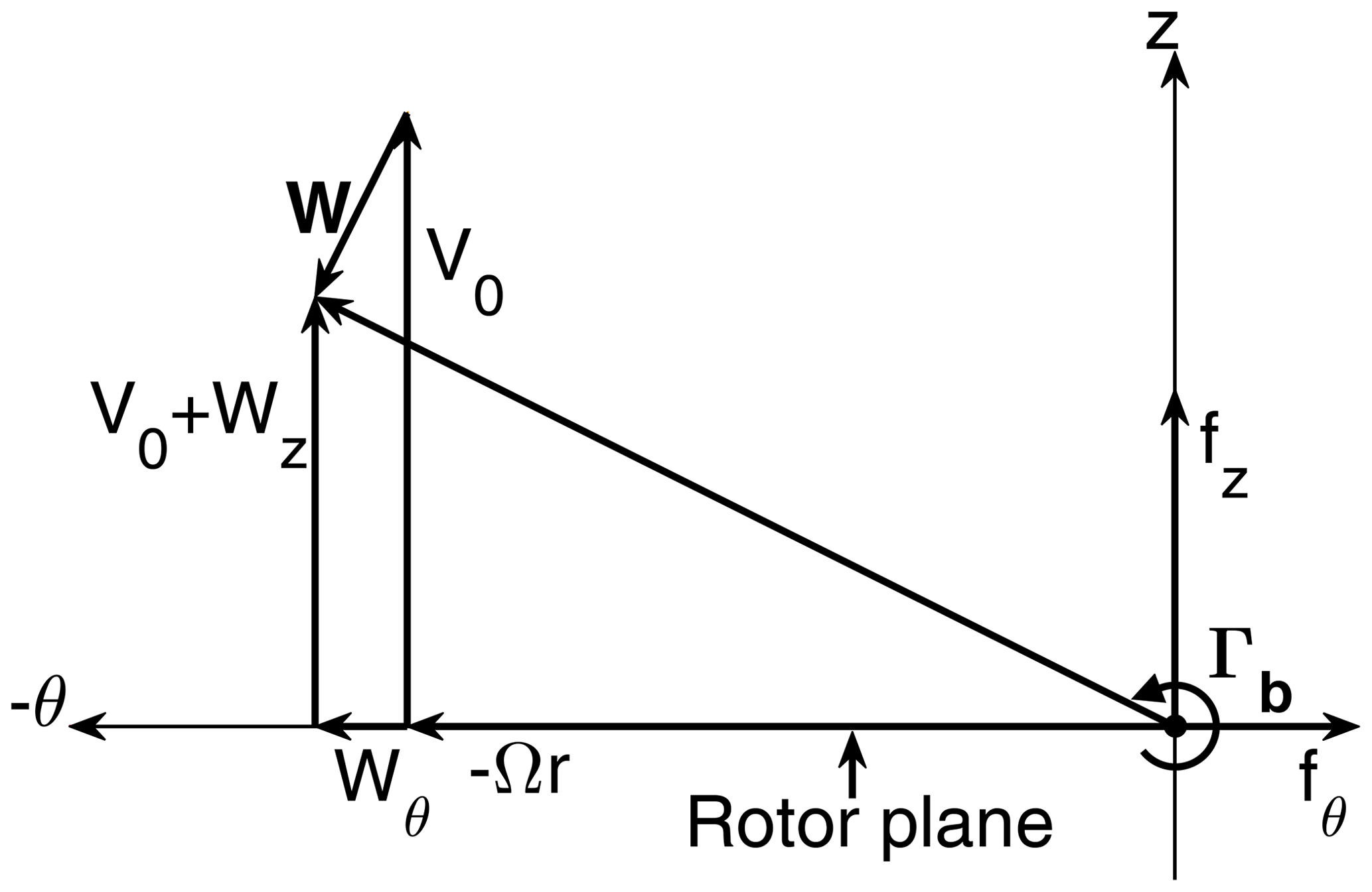
Figure 1Cross-section of blade element showing velocity and force vectors. The blade is pointing out of the paper, and the considered cross-section is located at the origin of the coordinate system.
In the case where the bound circulation is allowed to vary not only as a function of the radius, r, but also as a function of the azimuth location, θ, it is noted that the local thrust coefficient, Eq. (4), and the local power coefficient, Eq. (6) (and/or Eq. 7), remain unchanged. In this more general loading case, it is noted that the physical interpretation of the local quantity Γ(r,θ) is the amount of bound blade/rotor circulation that passes the rotor disc location (r,θ) during one revolution of the rotor. It is noted that the local Γ(r,θ) is not equal to the azimuthal sum of the bound vortex strengths at radius r: no azimuthal averaging is required to obtain the local Γ(r,θ). The general local definition of Γ is used in the remainder of this work.
2.1.2 Wake vorticity
In order to determine the velocity at the rotor disc and in the wake of the disc, the strength of the trailed and shed vortex sheets downstream of the disc is needed. To do this, we will be using the following result, which is proven in Appendix A and illustrated in Fig. 2:
For an infinitely long extruded surface of constant-strength tangential vorticity, , the induction in the direction of the extrusion axis (z) is γ on the inside and zero on the outside of the surface irrespective of its cross-sectional shape. Due to the symmetric properties of vortices, the axial induction at the ending plane of a corresponding half-infinite extruded vortex surface is .
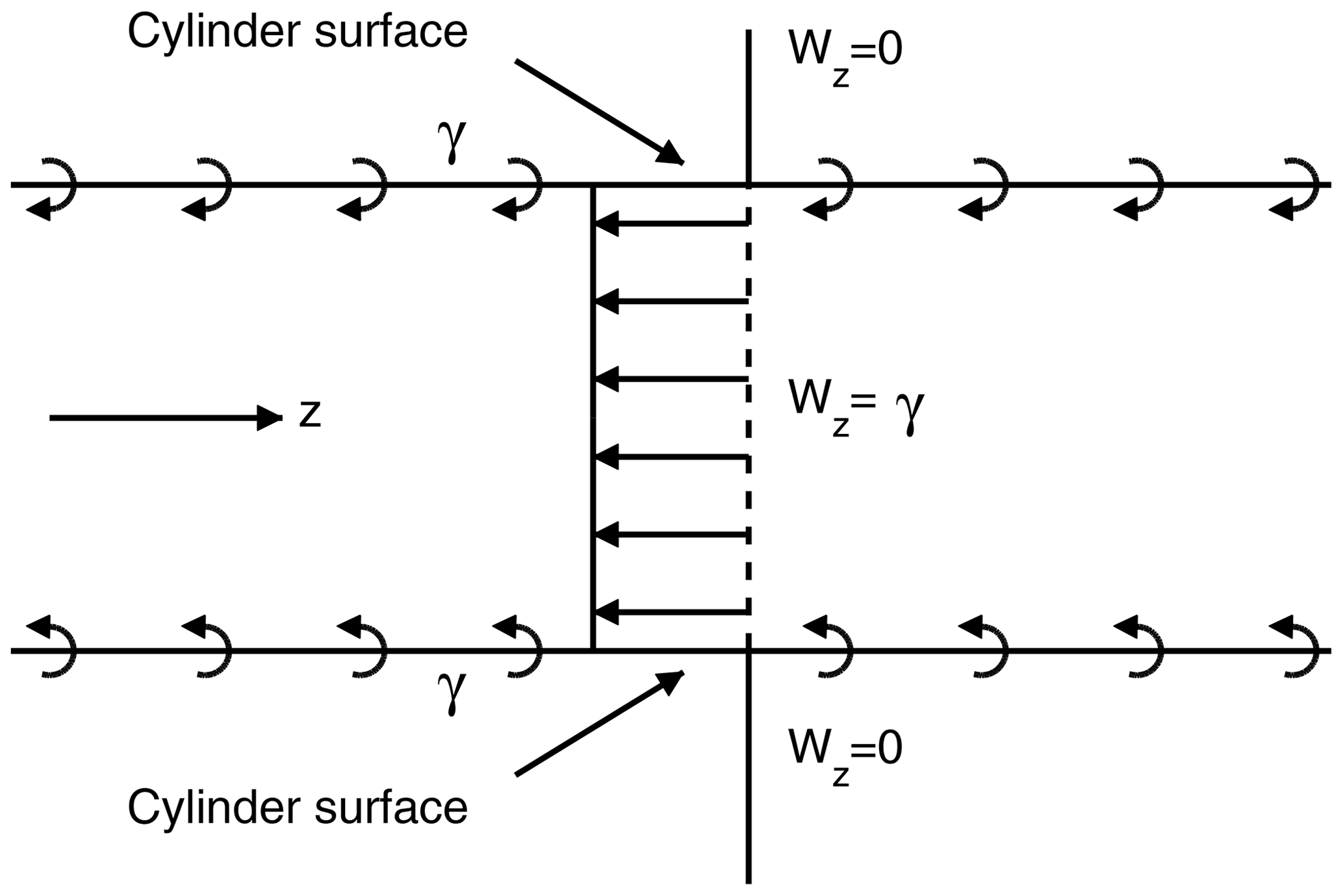
Figure 2Sketch of velocity field induced by an infinitely long extruded surface of tangential vortex density γ.
According to Helmholtz's first law, all vortex lines must form closed loops, extend to infinity or start/end at solid boundaries. Therefore, any change in bound vorticity in the radial direction causes vorticity to be trailed into the wake from the rotor, while variations in the bound vorticity in the tangential direction result in vorticity shed into the wake (see Figs. 3 and 4, where a discrete representation of the circulation is used for a finite tip speed ratio to simplify the discussion). It is shown in Appendix B that if the local bound vorticity Γ on the blade changes from position i to j on the rotor, the strength of the trailed and/or shed vorticity is given by
Here ΔΓ denotes the difference in local bound circulation between locations i and j, and is the transport velocity of the vorticity sheet in the axial direction. From Eq. (8), it is clear that to determine the strength of the trailed and shed vortex sheets, the convection velocity is needed. This convection velocity is the mean of the velocities on each side (above and below) of the vortex sheet. In order to simplify the present model, we adopt a generalization of what was shown by Øye (1990) to give good results: a vortex sheet is convected with a constant velocity which is the mean of the velocity on each side of the sheet far downstream of the rotor. Given two regions i and j, the convection velocity is therefore , where and are the velocities on each side of the vorticity sheet far downstream of the rotor.
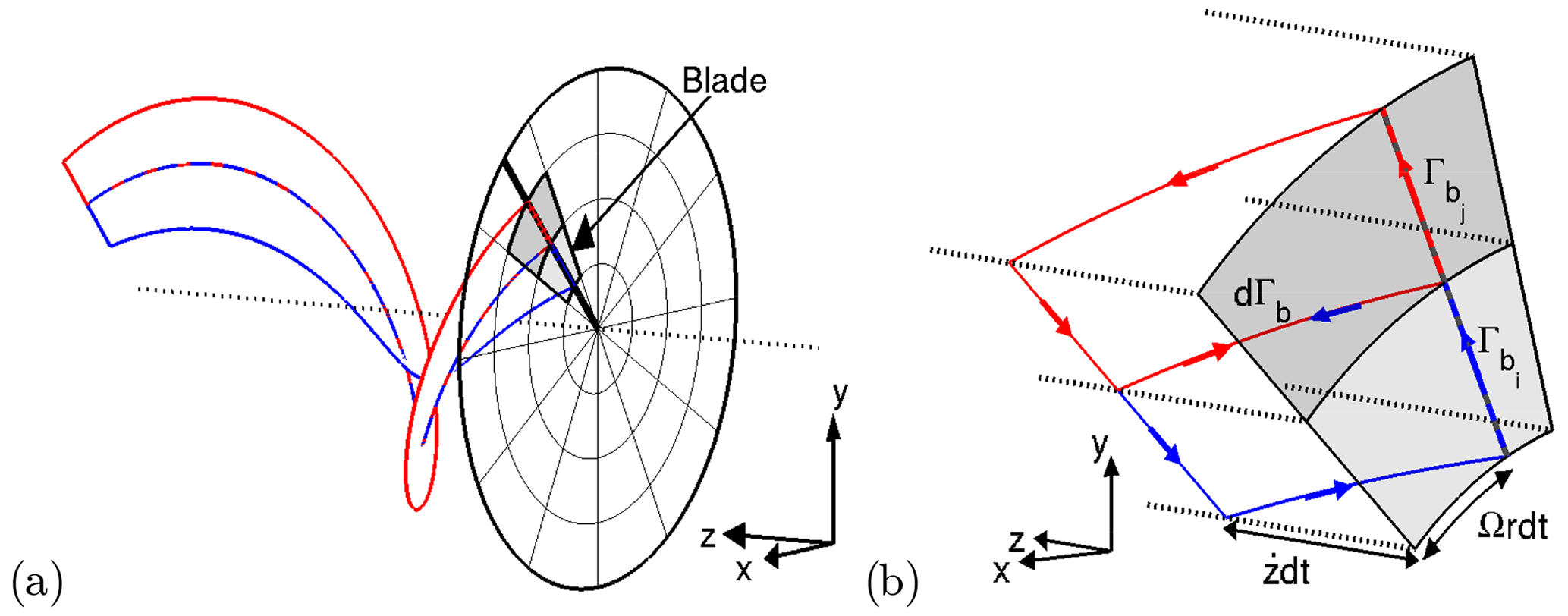
Figure 3(a) Sketch of vorticity trailed from a blade section, when the bound vorticity changes by in the radial direction. (b) Close view of the blade section showing the definition of dΓb.
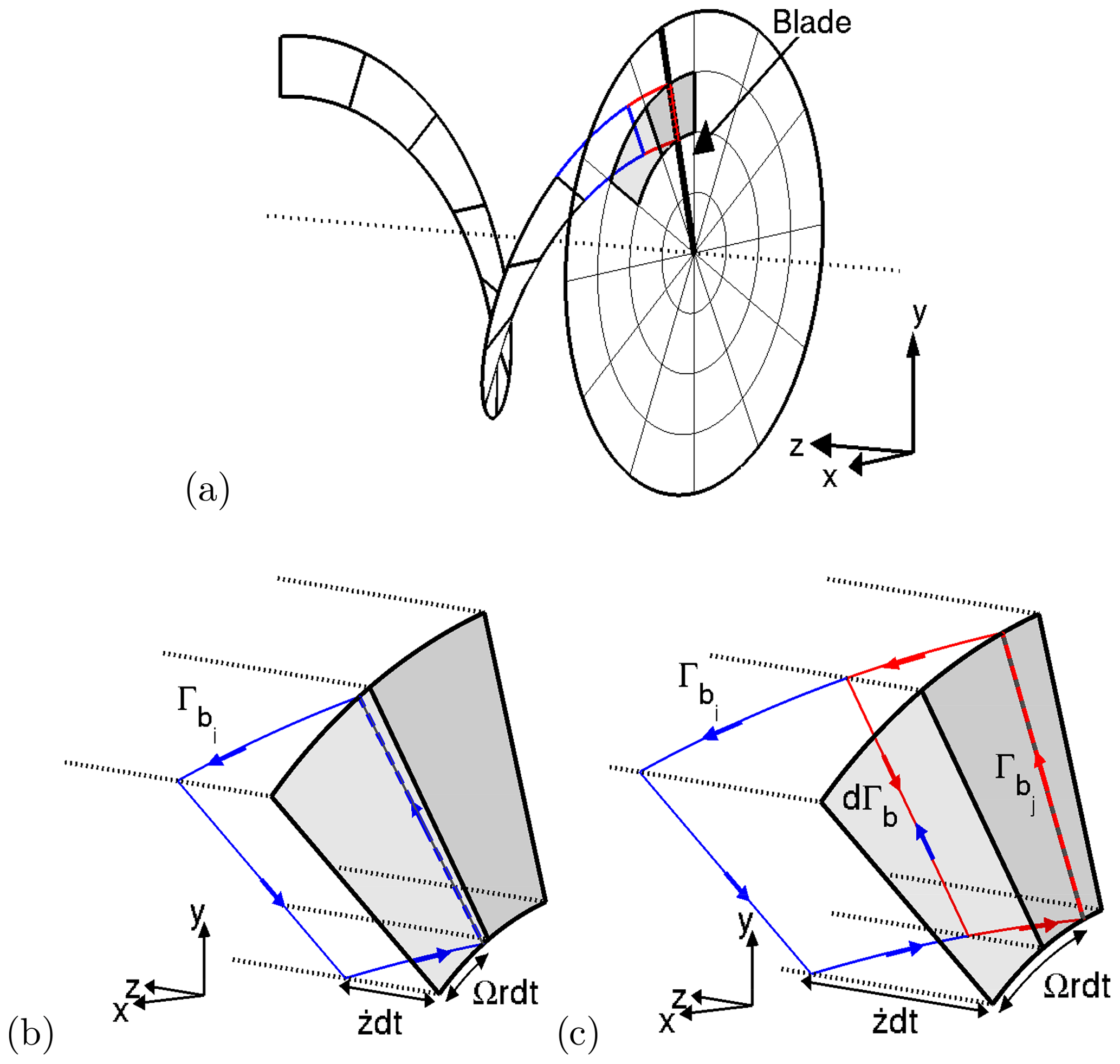
Figure 4(a) Sketch of vorticity shed from a blade section, when the bound vorticity changes in the tangential direction. (b, c) Close view of the blade section at two successive time instances, showing the definition of dΓb.
Using this assumption together with Eqs. (4) and (8), the strength of the vorticity sheet released into the wake as a consequence of a local change in loading between two regions i and j on the disc can be expressed as follows:
where and denote the local thrust coefficient of the two regions, respectively, and and are their corresponding local free-stream velocities.
3.1 Uniformly loaded rotor in uniform inflow
In this section, we consider a uniformly loaded rotor in uniform inflow. In this case, all the bound vorticity of the disc is trailed from the edge of the disc, and thus the vorticity released into the wake is distributed on a cylinder as sketched in Fig. 5. The strength of the released vorticity sheet, γ0−1, is determined from Eq. (9) and using the assumptions described in Sect. 2.1.2:
where is the thrust coefficient of the disc, is the free-stream velocity and the subscript 0−1 indicates that the vorticity is released between the wake (region 1) and the exterior (region 0). Solving for γ0−1 yields
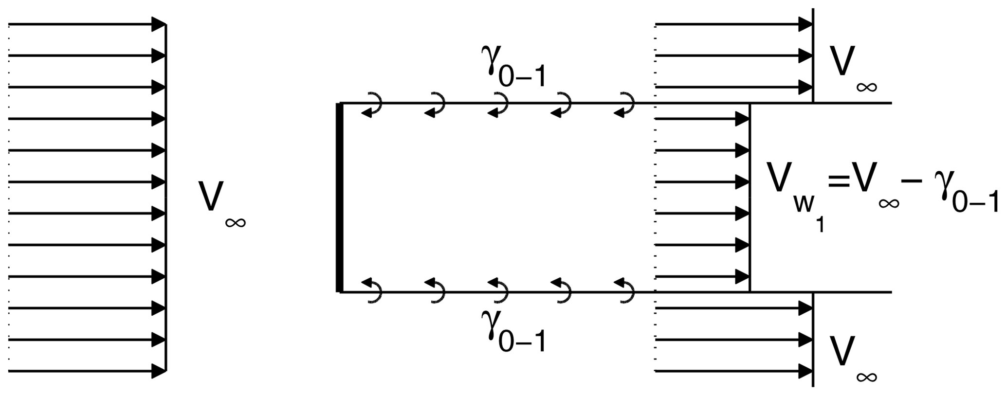
The rotor disc is at the ending plane of a half-infinite vortex cylinder and thus as described in Sect. 2.1.2; the axial velocity here is , where a is the axial induction factor. Therefore , and from Eq. (11), we get
where Vw is the velocity in the far wake.
Equations (12) and (7) show that the present model and classical 1D momentum theory give identical results. This is consistent with the conclusion drawn by Øye (1990) and shows that the crude approximations made herein are essentially not worse than the assumptions made in 1D momentum theory.
3.2 Non-uniformly loaded rotor in uniform flow
In this section, we apply the model to a non-uniformly loaded rotor in uniform flow. For simplicity we consider a case where two different load levels are present: in the lower half of the rotor disc and in the upper half; see Fig. 6. We start by assuming that the axial velocity in the far wake (and therefore also at the rotor disc) is constant in each of the two regions and then later check whether this assumption leads to inconsistencies.
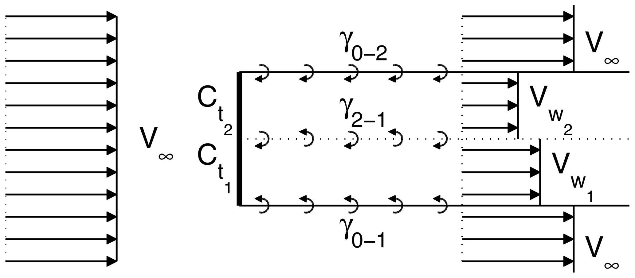
If the axial velocity in each of the far-wake regions is constant, its value should be as in the uniformly loaded case, since at the outer edge, the local conditions are as in the uniformly loaded case. Thus, the far-wake velocity in each region would be given by Eq. (13) and the strength of the sheet released between the two regions would be given by Eq. (9); i.e.
In order to have a constant velocity in the wake of each zone, this vortex sheet strength should, according to the behaviour of extruded vortex surfaces (Sect. 2.1.2), be equal to the difference in the “outer” vortex sheet strengths of each zone. From Eq. (11) the difference in sheet strengths between the regions from 1 and 2 to the exterior is
This is exactly equal to Eq. (14). If the assumption of a constant velocity in each of the two zones were incorrect, this would not have been the case. The arguments used in the derivation above also hold in the general case with more than two different load regions including cases where one load region is fully enclosed in other load regions. Therefore, the present model predicts that any stream element behaves locally as predicted by 1D momentum theory. This is in agreement with the result presented by Johnson (2013) and Branlard and Gaunaa (2015) and consistent with the derivation of the classical axisymmetric blade element theory, where the annular stream tubes are assumed to be independent of each other. However, the present model goes further as it indicates both radial and tangential independence of the individual stream elements. Thus, while one might expect that more air would flow through a lightly loaded part of a non-uniformly loaded rotor in uniform inflow, the present model predicts that this is not the case. Otherwise, the axial velocity (and hence power production; see Eq. 6) on the lighter loaded part of the disc would be higher than what is expected from 1D momentum results.
3.3 Non-uniformly loaded rotor in a step shear
We now consider a non-uniformly loaded rotor in a planar step-shear inflow, as illustrated in Fig. 7. A 3D sketch of the case is shown in Fig. 8, which outlines the different vortex strength contributions. For simplicity, we assume that the rotor has a constant loading of below the step and another constant loading of above the step. A step shear can be obtained by adding an infinite planar vortex sheet and a uniform flow. Note that such a sheet is consistent with Helmholtz's theorem because it starts and ends at infinity. If γs denotes the shear sheet strength and V∞ denotes the uniform free-stream speed, we get the following far-field, upstream inflow velocities:
where y denotes the height above the shear vorticity sheet. The main effect of the rotor is to change the axial velocity of the flow and hence also the convection velocity of the shear sheet in the wake.
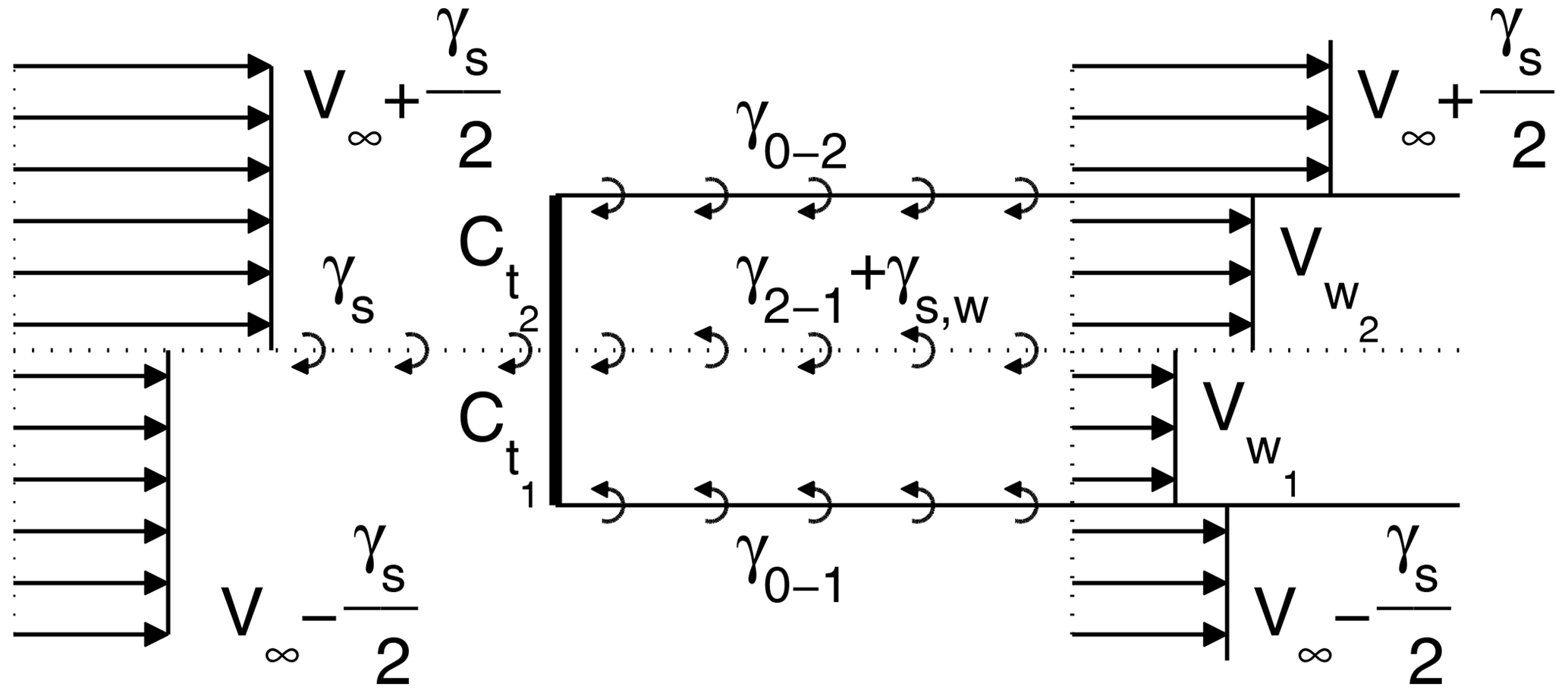
Figure 7Schematic view of a non-uniformly loaded disc in a step shear generated by introducing an infinite vorticity sheet of strength γs in the horizontal plane through the rotor centre.
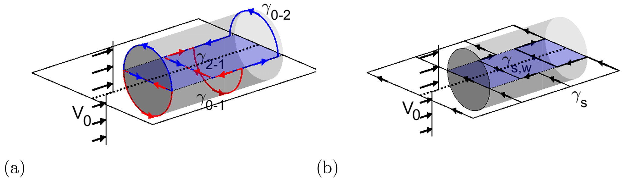
Figure 8A 3D sketch of a non-uniformly loaded disc in a step shear with illustration of the deformation of wake and shear vorticity sheets: (a) deformation of wake vortex rings and (b) deformation of the vortex filaments which are responsible for the step shear.
Due to steady-state conditions, the transport of circulation through any point in the shear plane is equal to that far upstream:
where is the mean of the far-wake velocities on each side of the shear vorticity layer and γs,w is the intensity of the shear vorticity sheet in the wake. Thus, for a wind turbine the intensity of the shear vorticity sheet is effectively increased in the wake because the axial velocity is lower than in the free stream.
For convenience, the intensity of the shear vorticity sheet in the wake is split as follows:
where γs is responsible for the effective backbone velocity (Eq. 16) and Δγs is the additional induced part due to the changed velocity in the wake.
In order to check whether our model is also consistent with 1D momentum theory in the sheared inflow case, we proceed as in the previous section and assume that the induced velocities in each region are constant and see whether this leads to any inconsistencies.
If the axial velocity in each of the far-wake regions is constant, it should be determined from Eq. (13), where now the local backbone free-stream velocity has to be used.
where index i=1 and i=2 refer to the two regions, respectively, and where we have introduced the local induction factor for region i:
Inserting Eq. (19) into Eq. (9) yields the following expressions for the strength of the vortex sheets released from the rotor:
Similarly, by inserting Eq. (19) into Eq. (17) and using Eq. (18), we get the following expression for the additional induced shear vorticity:
In the far wake, the intensity of the vortex sheet separating the upper and lower part of the wake is
Inserting Eqs. (23) and (24) into Eq. (25) and rewriting using Eq. (19) yields
From the basic behaviour of extruded vortex surfaces (Sect. 2.1.2), we know that in order to have a constant induced velocity in the wakes of each of the zones, the total vortex sheet strength between the lower and upper zones is equal to the difference in the outer vortex sheet strengths of each zone. From Eqs. (21) and (22) we get
As seen, Eqs. (27) and (26) are identical. Therefore, the initial assumption of a uniform far-wake velocity in each region was correct.
The reason why there is no local effect of the shear is that the effect of the changed convection velocity of the wake vorticity (), at the shear intersection, is exactly counterweighed by the induced shear vorticity (Eq. 24).
From Eqs. (20) and (7) we get the local thrust and power coefficient:
which are identical to the classical result from 1D momentum theory. In analogy with the arguments given in the previous section, we conclude that local 1D momentum theory is valid for any load distribution and any 1D shear, under the assumptions made in this work. This is an important result to keep in mind when developing additions to BEM models to make them able to perform sensibly in shear, since it shows that such models should be based on local quantities and avoid adopting concepts such as average disc load/induction or average annulus load/induction.
3.4 Formation of cross-shear-induced velocities
A basic property of vortex filaments in inviscid flow is that they cannot end in the fluid, and therefore both the wake and shear vorticity sheets are deformed under the influence of velocity gradients. This is illustrated in Fig. 8, which is a 3D sketch of the same non-uniformly loaded disc in a step shear as was considered in Sect. 3.3. Figure 8a sketches the shape of the individual wake vortex rings at the position of the rotor and in the wake, respectively. As a consequence of the shear and/or the difference in loading between the two regions of the rotor, the outer part of the vortex rings moves with another velocity compared to the part at their intersection, and therefore the vortex rings will be increasingly stretched with downstream position.
The stretching of the shear vorticity sheet is illustrated in Fig. 8b. Upstream of the rotor the entire span of the infinitely long shear layer vortex filaments is convected with the same velocity, and therefore the vortex filaments remain straight here. Downstream of the rotor, they will be deformed at the wake edges because of the difference in velocity inside and outside of the wake.
Due to the stretching of the wake and shear layer vorticity sheets, axial vorticity is formed at the intersection between the shear vorticity layer and the edges of the wake. However, from Fig. 8 it is evident that axial vorticity is generated in opposing directions: the upper-wake vortex rings are responsible for producing axial vorticity in the flow direction, whereas the opposite is true for the lower-wake vortex rings and the shear layer vorticity sheets. Nevertheless, if there is a net production of axial vorticity in one direction, this will induce a velocity component perpendicular to the flow direction. This in turn will cause the shear layer and wake vorticity sheets to be deflected in the direction perpendicular to the flow direction and thus result in different velocities on the rotor than would have been the case if the axial vorticity production had been neglected. In the following we will therefore use our model to calculate the total axial vorticity produced by the interaction of the wake and the shear.
3.4.1 Axial vorticity from wake–shear interaction
The axial vorticity at a given streamwise position z can be calculated by considering the conservation of vorticity for an infinitesimal cylindrical control volume enclosing the junction between the wake border and the shear sheet layer from 0 to z as shown in Fig. 9. Since all vortex filaments form closed loops or start and end at infinity, it is clear that the total flux of γ through this control volume is zero. Therefore, the axial vorticity through the end faces of the control volume is in balance with the vorticity through its sides. Thus, the axial vorticity can be determined by integrating the vorticity entering and exiting the sides of the control volume from 0 to z.

Figure 9(a) A 3D sketch of the control volume used for computing the axial vorticity. (b, c) Front view with outline of the tangential vorticity stemming from the wake (b) and shear (c).
The contribution from the wake stretching is then
where γ0−1, γ0−2 and γ2−1 are the strength of the vorticity sheets released from the rotor and are determined from Eqs. (21)–(23).
The corresponding contribution from the deformation of the shear layer vorticity sheet is
where Δγs is defined in Eq. (24).
From Eqs. (26) and (27) we know that
From Eq. (32) it is clear that Eqs. (30) and (31) exactly balance each other out, and therefore there is no net production of axial vorticity, which means that the present model predicts that there is no vertical movement of the wake and hence also no change in the power coefficient for a non-uniformly loaded rotor in sheared inflow. Note that the result of no net production of axial vorticity is general, which means that it also holds in the case without shear.
In the following we will relate the results of our model to the findings of the aforementioned literature.
The conclusion that the power coefficient (defined in terms of the actual available power) of an idealized rotor is unaltered by the presence of a 1D shear is in agreement with the CFD simulation by Zahle and Sørensen (2010) as well as the work by Chamorro and Arndt (2013). However, in contrast to the latter study, we do not assume self-similarity between the velocity profiles far upstream and downstream in order to arrive at this result. Furthermore, our conclusion is based on a generic study, whereas the simulations by Zahle and Sørensen (2010) were carried out on a specific rotor, and hence it is unknown to what extent their findings depend on the rotor and operational conditions used.
Since our model does not predict any formation of axial vorticity, it also does not predict a vertical deflection of the wake, which is in agreement with the studies by Branlard et al. (2015) and Ramos-García et al. (2018). In the CFD simulation by Zahle and Sørensen (2010), this effect is implicitly included, and the downward velocity component that they observe upstream of the rotor is an indication that axial vorticity is in fact generated in the wake. This suggests that an ideal rotor might actually get a higher power coefficient in sheared inflow. The production of axial vorticity could be included in our model by assuming the transport velocity of the wake vorticity changes gradually from its value at the disc to that in the far wake. The absence of vertical motion of the wake as predicted by our method is in agreement with what would be found from a momentum analysis of the same situation: there are no vertical forces acting from the rotor on the flow2, and therefore a control volume analysis of momentum conservation would show no vertical displacement of the wake.
Our model is based on several simplifying assumptions as outlined in Sect. 2, and the above findings should of course be seen in this light. Most of the assumptions made about the rotor are fairly standard for engineering analyses, and we do not expect that a more advanced rotor representation would change the overall findings of our model. Nevertheless, a consequence of assuming an infinite tip speed ratio is that rotational effects are neglected, and hence any impact of asymmetric development of the wake in sheared inflow is disregarded by our model. The effect of a finite tip speed for axisymmetrically loaded rotors in uniform inflow was assessed in Branlard and Gaunaa (2016) using a model based on the same building blocks as the present work. This work showed that the effect of the finite tip speed ratio is a second-order effect for tip speed ratios typically used in modern wind turbines. Therefore, we expect that the impact of neglecting rotational effects is small for moderately sheared inflow and typical tip speed ratios of wind turbines.
On the other hand, out of the assumptions made about the flow, e.g. incompressible potential flow, no wake expansion and constant transport velocity of wake vorticity, the latter two are obviously questionable. In reality the wake is clearly expanding and the transport velocity of the wake vorticity will be faster in the near wake than in the far wake. Thus, on their own these two assumptions are bad and lead to poor predictions. However, when used together the two assumptions lead to predictions that are consistent with 1D momentum theory. The reason for this is that while neglecting wake expansion leads to an underprediction of the induction in the rotor plane (Øye, 1990), the opposite is true when assuming a constant transport velocity of wake vorticity, and thereby the two assumptions counteract each other. The agreement with 1D momentum theory indicates that our model is of the same order of fidelity as those typically used in BEM models. However, our model gives another perspective and is developed for non-uniform inflow, and thereby it can be used to gain insight and guide future development of BEM models to correctly cope with sheared inflow.
We presented a simple analytical model based on inviscid vortex theory and applied it to model a rotor in uniform and non-uniform inflow.
Even though the model is based on a number of crude assumptions such as neglecting wake expansion and using a wake convection that is constant along each emission location, we showed that the model gives results that are identical to classical 1D momentum theory when applied to a uniformly loaded rotor operating in uniform inflow.
The application of the model to a non-uniformly loaded rotor operating in uniform inflow showed that any stream element through the rotor disc behaves locally as predicted by 1D momentum theory. Consequently, the model predicts that the stream elements through the disc are both radially and tangentially independent of each other.
For a non-uniformly loaded rotor operating in non-uniform inflow, our model predicts that the results from 1D momentum theory can be applied locally. Therefore, when the power coefficient is defined using the local free-stream velocity, we found that the power coefficient of an ideal rotor is unaltered by the presence of shear.
These findings indicate that the effects of shear and uneven loading in BEM-based codes should be treated in a local sense and that concepts such as average disc/annulus loading and induction should be avoided.
Finally, by studying the inherent deformation of the wake vorticity sheet and the wind shear vorticity sheet, we concluded that there is no net generation of axial vorticity. The effects of the deformation of the rotor wake vorticity due to the shear and effects of the deformation of the shear vorticity due to the rotor exactly cancel each other out. This means that there are no resulting cross-shear-induced velocities and therefore also no cross-shear deflection of the wake.
The result that the production of axial vorticity due to the deformation of the wake and shear vorticity cancelling each other out indicates that this effect has to be included in free-wake-vortex models. Omission of the effect of the deformation of the vorticity that creates the shear will result in a non-physical upward motion of the wind turbine wake in free-vortex models.
Consider an infinitely long extruded surface of tangential vorticity γ, which is aligned with the z axis and has an arbitrary cross-section; see Fig. A1. In the following we will show that this extruded vortex surface induces a velocity in the z direction of Wz=γ on the inside and zero on the outside of the surface.
The proof is carried out in steps by proving the following five statements:
-
The vortex surface only induces velocity in the z direction; i.e. .
-
The velocity is constant along z; i.e. .
-
The velocity inside and outside of the surface is constant and equal to and , respectively.
-
The outside velocity is .
-
The velocity inside of the surface is .
To prove the first statement, consider Fig. A2, which shows a lateral cut of the surface. By virtue of the Biot–Savart law, the velocity induced in a point P by a segment of the vortex surface is
where , pi is the vector from the segment to P and dsθ is an infinitesimal vector in the azimuth direction.
Now consider two segments on the vortex surface, which as shown in Fig. A2 are located at the same azimuth position, θ, but are located Δz and −Δz, respectively, from P. Due to symmetry, the radial velocities induced by these two segments cancel each other out. This holds true for any choice of azimuth position and ±Δz, and therefore it follows that the total induction of the vortex surface is in the z direction only. This can also be obtained by noting that each z plane is a plane of symmetry for the vorticity distribution so that the velocity has to be orthogonal to these planes.
The second statement follows from the invariance of the problem in the z direction, which implies that there is no dependence with respect to the variable z and the derivatives in the z direction are zero. This could have also been used to directly prove the first statement in the plane z=0.
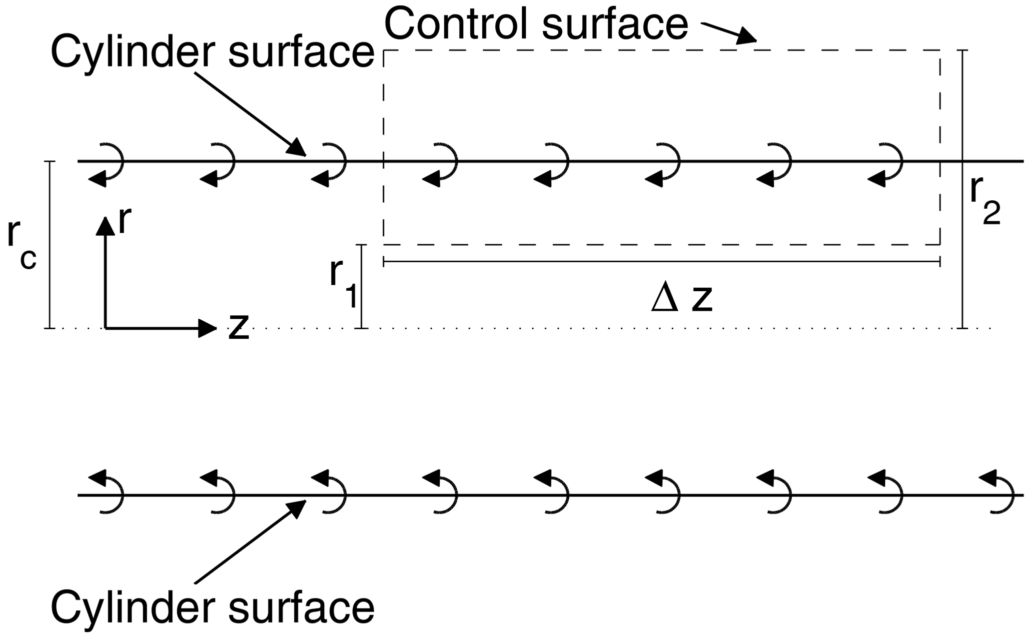
The third statement is proven by introducing a rectangular control surface as shown in Fig. A3. The length of the rectangle is denoted Δz, and its radial extent is from r1 to r2. Since the induction is only in the z direction, the circulation around the rectangle is
If the rectangle does not cross the vortex surface, then the circulation around the rectangle is zero. Thus it follows that for , whereas if .
The fourth statement follows by letting r2 go towards infinity where the induction from the vortex surface is 0; i.e. .
The fifth statement is proven by determining the circulation around the rectangular control surface when it is crossing the vortex surface and utilizing that ; i.e.
The induced velocity is thus independent of θ.

Figure A1Sketch of an infinitely long extruded surface of tangential vortex density γ with an arbitrary cross-section.

In order to derive Eq. (8), we use the assumption of a constant convection velocity of the vorticity surface in the longitudinal direction, denoted by .
First we consider the case where the jump in the local bound circulation occurs in the radial direction, as shown schematically in Fig. 3. The time it takes for the rotor to perform one revolution is . In this time span the amount of bound circulation passing zones i and j is the local Γi and Γj, respectively. The corresponding amount of circulation trailed between i and j in this time span is thus . During one rotor revolution, the trailed circulation is convected in the axial direction. Since the trailed vorticity is emitted at a constant rate in the intersection between i and j and the orientation of the trailed vorticity for tip speed ratios tending to infinity is practically parallel to the rotor plane, we get that the sheet strength of the azimuthally directed trailed vorticity between sections i and j is
Now we proceed to consider the case where the jump in bound circulation occur in the tangential direction, as shown in Fig. 4. The arguments in this case are analogue to the previous case. In this case is the shed circulation at the i–j border intersection during the time span of one rotor revolution (any circulation not carried onto zone j must be trailed due to Helmholtz's law). Since the time span for rotor revolution is the same as before, we arrive at an analogous result:
From the derivations it is evident that the relations for the sheet vorticity strength in both the radial and the tangential bound circulation change cases are identical. It can therefore be generally stated that the vorticity emitted at the border between two zones of different local bound circulation (or local thrust coefficients) is
No data sets were used in this article.
MG derived the model. NT wrote most of the manuscript and supported the analysis. EM contributed to the idea and derived the proof in Appendix A. All three reviewed and edited the manuscript.
The contact author has declared that none of the authors has any competing interests.
Publisher's note: Copernicus Publications remains neutral with regard to jurisdictional claims in published maps and institutional affiliations.
This work is funded by DTU Wind and Energy Systems.
This paper was edited by Roland Schmehl and reviewed by Joseph Saverin and Eduardo Alvarez.
Betz, A.: Das Maximum der theoretisch möglichen Ausnützung des Windes durch Windmotoren, Zeitschrift für das gesamte Turbinewesen, 26, 307–309, 1920. a
Boorsma, K., Schepers, G., Aagard Madsen, H., Pirrung, G., Sørensen, N., Bangga, G., Imiela, M., Grinderslev, C., Meyer Forsting, A., Shen, W. Z., Croce, A., Cacciola, S., Schaffarczyk, A. P., Lobo, B., Blondel, F., Gilbert, P., Boisard, R., Höning, L., Greco, L., Testa, C., Branlard, E., Jonkman, J., and Vijayakumar, G.: Progress in the validation of rotor aerodynamic codes using field data, Wind Energ. Sci., 8, 211–230, https://doi.org/10.5194/wes-8-211-2023, 2023. a
Branlard, E.: Wind Turbine Aerodynamics and Vorticity-Based Methods, Springer, https://doi.org/10.1007/978-3-319-55164-7, 2017. a
Branlard, E. and Gaunaa, M.: Cylindrical vortex wake model: right cylinder, Wind Energy, 18, 1973–1987, https://doi.org/10.1002/we.1800, 2015. a, b, c
Branlard, E. and Gaunaa, M.: Superposition of vortex cylinders for steady and unsteady simulation of rotors of finite tip-speed ratio, Wind Energy, 19, 1307–1323, 2016. a, b
Branlard, E., Papadakis, G., Gaunaa, M., Winckelmans, G., and Larsen, T. J.: Aeroelastic large eddy simulations using vortex methods: unfrozen turbulent and sheared inflow, J. Phys. Conf. Ser., 625, 012019, https://doi.org/10.1088/1742-6596/625/1/012019, 2015. a, b, c
Chamorro, L. P. and Arndt, R.: Non-uniform velocity distribution effect on the Betz–Joukowsky limit, Wind Energy, 16, 279–282, https://doi.org/10.1002/we.549, 2013. a, b
Glauert, H.: Airplane Propellers, in: Aerodynamic Theory, Vol. IV, Division L, edited by: Durand, W. F., Springer, New York, 169–360, https://doi.org/10.1007/978-3-642-91487-4_3, 1963. a
Grasso, F.: Ground and Wind Shear Effects in Aerodynamic Calculations, Tech. Rep. ECN-E–10-016, ECN – Energy research center of the Netherlands, https://www.researchgate.net/profile/Francesco-Grasso (last access: 3 April 2023), 2010. a
Johnson, W.: Rotorcraft Aeromechanics, Cambridge Aerospace Series, Cambridge University Press, https://doi.org/10.1017/CBO9781139235655, 2013. a
Lanchester, F.: A contribution to the theory of propulsion and the screw propeller, Transaction of the Institute of Naval Architects, 56, 135–153, 1915. a
Madsen, H., Mikkelsen, R., Johansen, J., Bak, J., Øye, S., and Sørensen, N.: Inboard rotor/blade aerodynamics and its influence on blade design, in: Risø report Research in aeroelasticity EFP-2005, Tech. Rep. Risø-R-1559(EN), Risø, National Laboratory, https://orbit.dtu.dk/en/publications/research-in-aeroelasticity-efp-2005 (last access: 3 April 2023), 2006. a
Madsen, H. A., Riziotis, V., Zahle, F., Hansen, M., Snel, H., Grasso, F., Larsen, T., Politis, E., and Rasmussen, F.: Blade element momentum modeling of inflow with shear in comparison with advanced model results, Wind Energy, 15, 63–81, https://doi.org/10.1002/we.493, 2012. a, b
Magnusson, M.: Near-wake behaviour of wind turbines, J. Wind Eng. Ind. Aerod., 80, 147–167, https://doi.org/10.1016/S0167-6105(98)00125-1, 1999. a
Micallef, D., Ferreira, C., Sant, T., and van Bussel, G.: An Analytical Model of Wake Deflection Due to Shear Flow, in: 3rd Conference on The science of making Torque from Wind, 28–30 June 2010, Crete, Greece, 337–347, https://repository.tudelft.nl/islandora/object/uuid:7b821f51-8fd7-43ee-aedf-1bbd3a3e6b542010 (last access: 3 April 2023), 2010. a
Øye, S.: A simple vortex model, in: Proc. of the third IEA Symposium on the Aerodynamics of Wind Turbines, ETSU, 16–17 November 1989, Harwell, UK, 70–73, NTIS Issue number 199106, 1990. a, b, c, d, e
Ramos-García, N., Spietz, H. J., Sørensen, J. N., and Walther, J. H.: Vortex simulations of wind turbines operating in atmospheric conditions using a prescribed velocity-vorticity boundary layer model, Wind Energy, 21, 1216–1231, https://doi.org/10.1002/we.2225, 2018. a, b
Sezer-Uzol, N. and Uzol, O.: Effect of steady and transient wind shear on the wake structure and performance of a horizontal axis wind turbine rotor, Wind Energy, 16, 1–17, https://doi.org/10.1002/we.514, 2013. a, b
Shen, X., Zhu, X., and Du, Z.: Wind turbine aerodynamics and loads control in wind shear flow, Energy, 36, 1424–1434, https://doi.org/10.1016/j.energy.2011.01.028, 2011. a
Troldborg, N., Sørensen, J., Mikkelsen, R., and Sørensen, N.: A simple atmospheric boundary layer model applied to large eddy simulations of wind turbine wakes, Wind Energy, 17, 657–669, https://doi.org/10.1002/we.1608, 2014. a
Zahle, F. and Sørensen, N.: Navier-Stokes Rotor Flow Simulations with Dynamic Inflow, Torque Conference, 28–30 June 2010, Crete, Greece, 2010. a, b, c, d, e
- Abstract
- Introduction
- A simple vortex rotor model including shear
- Application of model
- Discussion
- Conclusions
- Appendix A: Induction of an infinitely long extruded surface of tangential vorticity
- Appendix B: Detailed derivation of Eq. (8)
- Data availability
- Author contributions
- Competing interests
- Disclaimer
- Financial support
- Review statement
- References