the Creative Commons Attribution 4.0 License.
the Creative Commons Attribution 4.0 License.
 | 26 Apr 2023
An investigation of spatial wind direction variability and its consideration in engineering models
Anna von Brandis
Gabriele Centurelli
Jonas Schmidt
Lukas Vollmer
Bughsin' Djath
Martin Dörenkämper
We propose that considering mesoscale wind direction changes in the computation of wind farm cluster wakes could reduce the uncertainty of engineering wake modeling tools. The relevance of mesoscale wind direction changes is investigated using a wind climatology of the German Bight area covering 30 years, derived from the New European Wind Atlas (NEWA). Furthermore, we present a new solution for engineering modeling tools that accounts for the effect of such changes on the propagation of cluster wakes. The mesoscale wind direction changes relevant to the operation of wind farm clusters in the German Bight are found to exceed 11∘ in 50 % of all cases. Particularly in the lower partial load range, which is associated with strong wake formation, the wind direction changes are the most pronounced, with quartiles reaching up to 20∘. Especially on a horizontal scale of several tens of kilometers to 100 km, wind direction changes are relevant. Both the temporal and spatial scales at which large wind direction changes occur depend on the presence of synoptic pressure systems. Furthermore, atmospheric conditions which promote far-reaching wakes were found to align with a strong turning in 14.6 % of the cases. In order to capture these mesoscale wind direction changes in engineering model tools, a wake propagation model was implemented in the Fraunhofer IWES wind farm and wake modeling software flappy (Farm Layout Program in Python). The propagation model derives streamlines from the horizontal velocity field and forces the single turbine wakes along these streamlines. This model has been qualitatively evaluated by simulating the flow around wind farm clusters in the German Bight with data from the mesoscale atlas of the NEWA and comparing the results to synthetic aperture radar (SAR) measurements for selected situations. The comparison reveals that the flow patterns are in good agreement if the underlying mesoscale data capture the velocity field well. For such cases, the new model provides an improvement compared to the baseline approach of engineering models, which assumes a straight-line propagation of wakes. The streamline and the baseline models have been further compared in terms of their quantitative effect on the energy yield. Simulating two neighboring wind farm clusters over a time period of 10 years, it is found that there are no significant differences across the models when computing the total energy yield of both clusters. However, extracting the wake effect of one cluster on the other, the two models show a difference of about 1 %. Even greater differences are commonly observed when comparing single situations. Therefore, we claim that the model has the potential to reduce uncertainty in applications such as site assessment and short-term power forecasting.
- Article
(7260 KB) - Full-text XML
- BibTeX
- EndNote


The “European Green Deal” targets to make Europe climate neutral by 2050. To reach this goal, a decarbonization of the energy system is necessary, where increasing offshore wind production will play a key role (European Commission, 2019). With planned installed capacities of 30 GW in 2030, 40 GW in 2035 and 70 GW in 2045 the new German government has three long-term goals for offshore wind farm expansion in their coalition agreement (SPD et al., 2021). As areas are limited, a most effective arrangement of wind farms is desired. Thus, offshore wind farms are typically grouped in wind farm clusters, which can be composed of several hundreds of turbines.
A recent study of large-scale wind farm expansion in the German Bight suggests that the efficiency decreases with an increasing density of installed capacity (Agora Energiewende, 2020). The comparatively smooth surface and less-turbulent conditions benefit the formation of far-reaching wakes. Thus, cluster wakes and their impact on the power production have received increasing attention over the past years, applying different measurement and modeling techniques (e.g., Christiansen and Hasager, 2005; Li and Lehner, 2013; Hasager et al., 2015b; Djath et al., 2018; Platis et al., 2018; Siedersleben et al., 2018; Ahsbahs et al., 2020; Cañadillas et al., 2020; Nygaard et al., 2020; Schneemann et al., 2020; Cañadillas et al., 2022).
Far-reaching wind farm and cluster wakes were observed in satellite synthetic aperture radar (Djath and Schulz-Stellenfleth, 2019) also in combination with scanning lidar (Jacobsen et al., 2015; Schneemann et al., 2020) and dual-Doppler radar (e.g., Ahsbahs et al., 2020), as well as airborne measurement data (Platis et al., 2018). Offshore wind farm wake deficits last particularly long under stable conditions, but far-reaching wakes were also found under neutral and weakly unstable conditions (e.g., Djath et al., 2018; Platis et al., 2020; Schneemann et al., 2020). For very constant wind directions aligning with stable atmospheric stratification, Cañadillas et al. (2020) report wake lengths exceeding 80 km. The magnitude of the wake deficit far downstream ranges from 25 % to 41 % of the wind velocity for a distance of 24 km and 21 % at 55 km downstream (Schneemann et al., 2020). In the German Bight, conditions that benefit far-reaching wakes are expected to have a probability of about 5 % (Platis et al., 2018). The occurrence of stable conditions benefiting far-reaching wakes is dependent on the wind direction. Therefore, the occurrence of stable conditions in the main wind direction sector should be taken into account for the layout optimization of wind farms (Emeis, 2018; Platis et al., 2018; Cañadillas et al., 2020).
It is well established that the wake of wind farms and wind farm clusters can impair the power production of downstream wind plants. Nygaard and Hansen (2016) report a decreasing power production in the front rows of a downstream wind farm. Meanwhile, Schneemann et al. (2020) observed an area of reduced power production in the center of the wake, while speed-up effects occurred at the edges during partial cluster wake conditions. While the length of wakes has been studied on the scale of wind farms and wind farm clusters, their propagation in a homogeneous atmospheric flow has been studied only on the single turbine to farm scale. Few studies have focused on the wake deflection imparted by Coriolis force effects: van der Laan et al. (2015) investigated the phenomenon using computational fluid dynamics (CFD) and concluded that considering the Coriolis force affects the prediction of farm losses due to wake shadowing. In a later work, van der Laan and Sørensen (2017) explained the clockwise turning of wind farm wakes by the entrainment of wind veer from above the farm due to the Ekman spiral. This was studied in more detail by Gadde and Stevens (2019) using large-eddy simulations (LESs) with the result that at the inflow of the wind farm a counterclockwise rotation in the wind flow is observed as a consequence of wind farm blockage and wind veer. Further downstream, the downward mixing of veered flow from above the wind farm causes a clockwise deviation that directly impacts the trajectory of the farm wake (Eriksson et al., 2019; Gadde and Stevens, 2019). Furthermore, Eriksson et al. (2019) investigated the impact on the power production of a downstream wind farm, showing a difference of 3 % in power production for a single flow case when including the terms associated with the Coriolis force.
The previously summarized studies show that it is relevant to further examine the advection of wakes on scales of several kilometers – the mesoscale – and account for it in engineering wake models as these are commonly used for yield estimations prior to and after wind farm construction. Despite the lower resolution when compared to microscale CFD simulations, they can assess a large variety of different inflow conditions in a very computationally efficient manner (Machefaux et al., 2015).
A grid-based approach to consider wake advection in heterogeneous background wind fields in the engineering model context was developed for FLORIS (FLOw Redirection and Induction in Steady State) (NREL, 2020). In the model the flow is calculated on a mesh, rotated around the center of the flow field according to the local wind direction prior to the wake calculation. A backward rotation projects the wind direction changes of the background flow onto the wake (Farrell et al., 2021).
In this study, we propose a grid-less approach that unlocks the computational benefits of using analytical engineering wake models that do not necessitate a grid to be resolved. The model is coupled with background wind fields from a mesoscale numeric weather model for taking into account wind direction changes on large scales. The difference in calculated annual energy production (AEP) between the model and a simplified model solution for heterogeneous background flow is compared for a real example case of two large wind farm clusters in the German Bight.
The recently published approach by Lanzilao and Meyers (2022) applies a methodology for deflecting the turbine wakes along the streamlines from a heterogeneous background flow field. In this study, we suggest the coupling of engineering wake models with mesoscale background wind fields for taking into account mesoscale wind direction changes and thus apply an approach similar to Lanzilao and Meyers (2022) but on larger scales. This allows us to demonstrate how the method works and to discuss its implications when simulating for AEP calculation or site assessment.
The main objectives of this study are (1) to evaluate the relevance of mesoscale wind direction changes taking the German Bight as example, (2) to propose a modeling approach at the scale of cluster wakes, (3) to implement this approach into an engineering model framework and (4) to investigate this approach on the scale of cluster wakes.
Section 2 describes the methods used for investigating the importance of mesoscale wind direction changes. Furthermore, the developed wake propagation model and the simulations performed for its validation are described. Section 3.1 then introduces the engineering wake model suite flappy (Farm Layout Program in Python) developed at the Fraunhofer IWES with which the simulations were conducted. Section 4 briefly describes the data used for evaluating the importance of mesoscale wind direction changes, as well as the simulation of the streamline model and its comparison with synthetic aperture radar (SAR) data. In Sect. 5, the results are presented and discussed, split into the investigation of the wind direction changes and the evaluation of the cluster wake propagation. Finally, the findings are summarized in Sect. 6.
In this section, we present the methods to investigate the relevance of mesoscale wind direction changes for different spatial (Sect. 2.1.1) and temporal scales (Sect. 2.1.2). A mechanism to simulate a wake propagation following the mesoscale wind direction changes in an engineering model context is introduced (Sect. 2.2).
2.1 Investigation of mesoscale wind direction changes
One aim of this study is to examine under which conditions large wind direction changes occur on the mesoscale. This evaluation is based on mesoscale model data originating from the New European Wind Atlas (NEWA) which are described in Sect. 4.1.
2.1.1 Spatial scales
For the investigation of the impact of mesoscale wind direction changes, we first define three different scales determined by the distance of prominent offshore locations (wind farms, an offshore substation and two meteorological masts) in the German Bight: the intra-cluster scale which corresponds to the distance between the offshore substation DolWin1 and the met mast FINO1, the inter-cluster scale defined by the distance between the wind farms Deutsche Bucht (DBU) and Global Tech I (GT I), and the German Bight scale by met masts FINO1 and FINO3. Figure 1 shows the locations and distances between these locations.
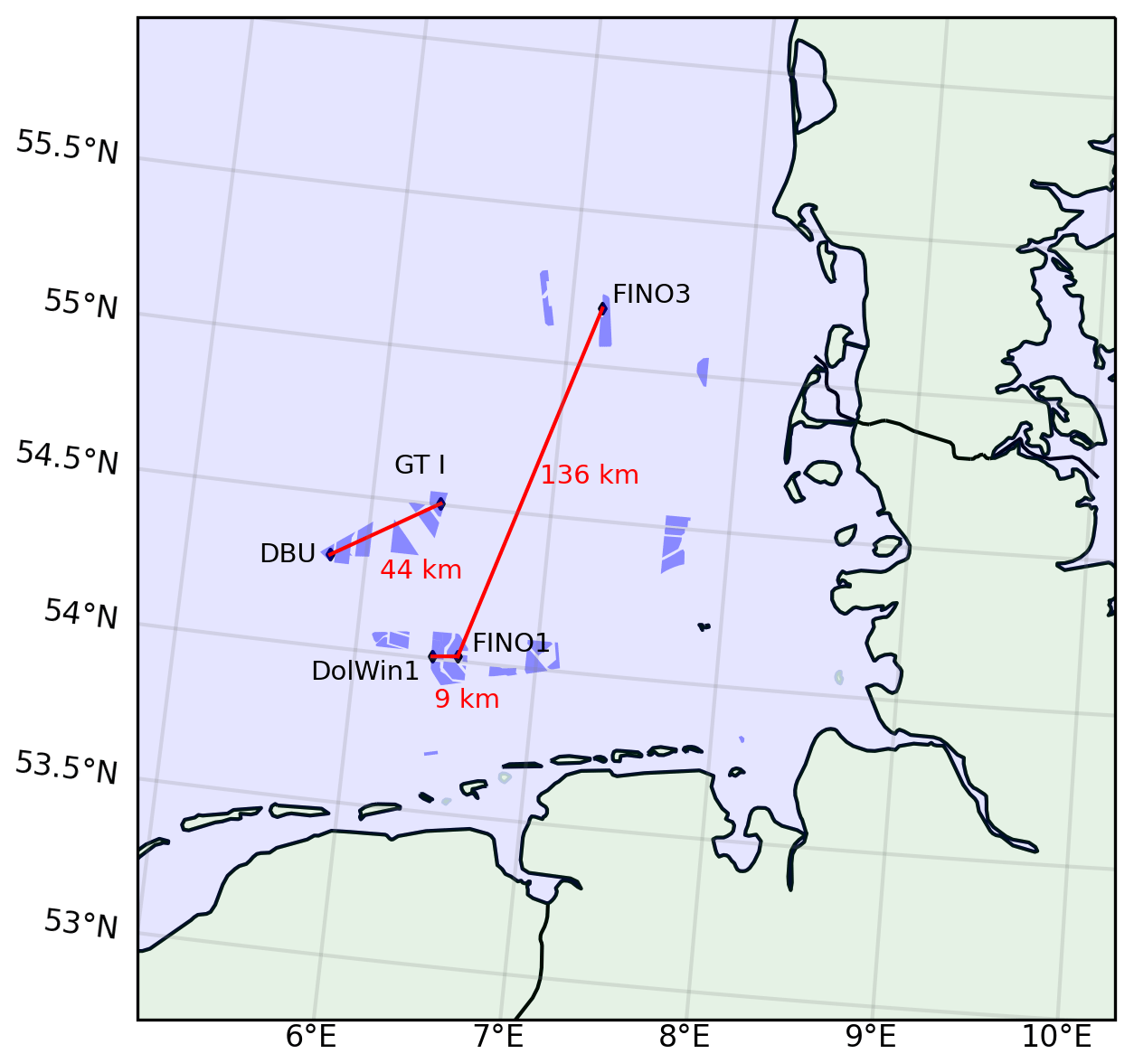
Figure 1Different scales in the German Bight: intra-cluster scale: DolWin1 and FINO1; inter-cluster scale: Deutsche Bucht (DBU) and Global Tech I (GT I); and German Bight scale: FINO1 and FINO3. For the evaluation, the NEWA grid points closest to the selected sites were taken. The wind farms that are currently operational and under construction are marked in blue (data from Bundesamt für Seeschifffahrt und Hydrographie, 2020). The coastline and border data originate from the Natural Earth dataset (Natural Earth, 2021).
The comparison of wind directions at different spatial scales was performed using mesoscale model time series of wind direction and speed at the grid points named above over a period of 30 years. The difference in wind direction between the two time series was calculated for each time step. To examine the dependency on the wind speed, they were then binned by the wind speeds at a reference location (WSREF):
with i∈n and n as the number of bins. A bin width of 2.5 m s−1 was chosen, as this was found to depict the dependency of wind direction change ΔWD on the wind speed while still reducing the number of bins to a reasonable amount. For each wind speed bin, the median, quartiles and the percentiles of wind direction differences were calculated.
In a second step, the whole German Bight area was investigated to examine the horizontal patterns of wind direction changes for a climatology of 30 years. The wind direction data were again binned by wind speed at the reference location, and the mean values of the yearly median, upper and lower quartiles of ΔWD at each grid point were calculated. The wind direction change was calculated as a difference in wind direction between each grid point Pj and the reference point PREF, and the statistical parameters described above were calculated:
In order to account for the distances to the reference location, the wind direction changes per 100 km were evaluated using the great circle distance between the Pj and PREF.
The area in Fig. 2 marked in gray was chosen for analyzing mean wind direction changes over the whole German Bight, as it excludes onshore sites. This area has a minimum distance to the nearest coastline of 5.3 km southwards and 7.7 km eastwards. After the mean of the yearly percentiles was taken for each grid point, the mean of the grid points in the offshore area was calculated. In all cases where wind direction differences were calculated, we accounted for the circular nature of the wind direction variable.
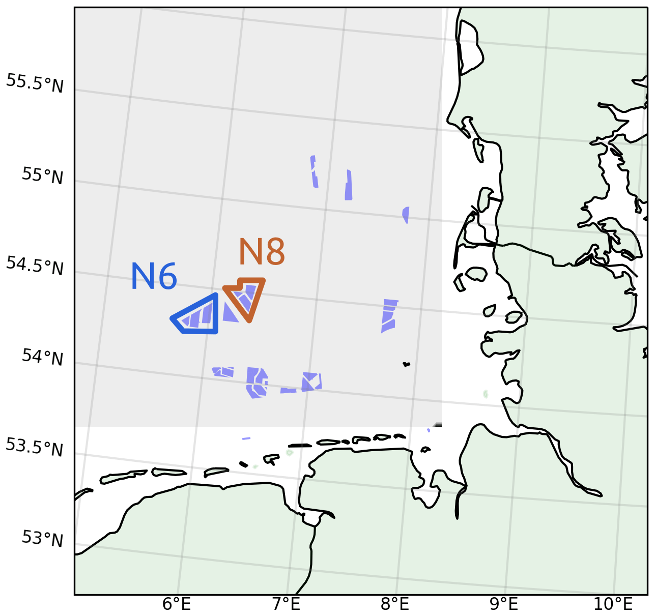
Figure 2German Bight, selected area for calculating mean wind direction changes. The wind farms currently commissioned and whose consent was authorized in the German Bight are marked in blue (data from Bundesamt für Seeschifffahrt und Hydrographie, 2020). The wind farms of the N6 cluster are framed in blue, whereas the ones of the N8 cluster are framed in orange. The coastline and border data originate from the Natural Earth dataset (Natural Earth, 2021).
2.1.2 Temporal scale: synoptic pressure systems
Wind direction changes are expected to be more pronounced on shorter timescales during the passage of synoptic pressure systems. Cyclones are usually transient and characterized by a strong curvature of the isobars. The passage of their frontal system is related to a drop in surface pressure and high wind speeds (Bott, 2016). Therefore, the wind direction changes were investigated for single cyclone events by choosing time frames of 2 d around time periods when wind speeds above 15 m s−1 were persisting at FINO1 for each event. Anticyclones in contrast are often prevailing over longer time periods and are often characterized by relatively constant high atmospheric pressure at the surface. Thus, the examined high-pressure situations were filtered by sea level pressure constantly exceeding 1020 hPa at FINO1. These conditions were found to last about 4 d in the selected examples. It has to be noted that in this part of the study, particularly pronounced synoptic pressure systems were investigated to examine extreme situations.
As before, the analysis was based on mesoscale model data. The wind direction at the mesoscale grid point closest to FINO1 was subtracted from the one at each grid point in the German Bight, and the resulting direction changes were visualized in maps. Furthermore, the mean wind direction change over these above-mentioned time frames was calculated for different spatial scales as shown in Fig. 1.
2.2 Implementation of mesoscale wind direction changes into engineering models
In order to capture the mesoscale wake advection in the background flow, we determine the coordinate transformation from the global Cartesian frame of reference to the wake frame of reference for each wake-causing turbine. The wake frame is defined as a right-handed orthonormal coordinate system whose first axis follows the streamline curve that is originating at the rotor center.
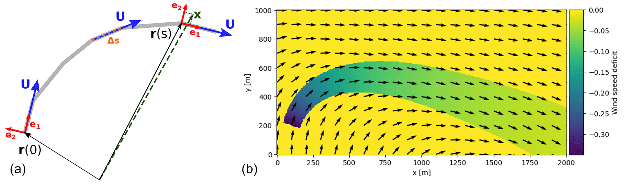
Figure 3(a) The thick gray line represents the piecewise linear streamline, as obtained from the steady-state flow field U based on the selected time step Δt. The wake-causing rotor is located at position r(0). Each segment has its own local coordinate system, indicated by the red vectors e1, e2. Here x denotes the point of wake model evaluation, and r(s) is the nearest support point of the discretized streamline. (b) An example outcome for the Jensen wake model in a wind field with rotation.
For the wake calculations, our method considers any time step in the mesoscale time series as an independent heterogeneous steady-state flow field. Denoting the latter as U(x), the path r(t) of a probe particle moving in this background flow field is determined by the first-order differential equation . For the formulation of the streamline we choose a parametrization by the distance s along the path rather than the time t, implying . Using this relation we can replace the dependency of the position vector r along the streamline on the traveling time t by a dependency on the traveled distance s, starting at the wake-causing rotor. Doing so, we obtain the differential equation for the streamline curve r(s):
At any point of the streamline the normalized local tangent vector induces a right-handed orthonormal coordinate system with axes e1, e2, e3:
where ez is the Cartesian direction vector in the z direction. For any point x at which the wake model is to be evaluated, we are now in the position to define wake frame coordinates (c1, c2, c3) representing the stream-wise, orthogonal and vertical directions, respectively, by
Equation (3) is then solved in discretized form for each rotor, with r(0) representing the rotor center. For each location x Eqs. (4) and (5) are then computed at the nearest point of the resulting piecewise linear streamline; see Fig. 3. Finally, the wake model equations are evaluated based on the resulting coordinates (Eq. 5).
In this section, we introduce the Fraunhofer engineering model suite (Sect. 3.1), as well as its setups used for the simulations presented in this study (Sect. 3.2).
3.1 The Fraunhofer engineering model suite
All wind farm and wake calculation results in this work were obtained using the Farm Layout Program in Python (flappy; version v0.5.2) developed by Fraunhofer IWES. This code is based on grid-less wake model superposition, and it has been optimized for numerous input states, like long-term time series or statistical distributions. The flappy software has recently been applied to very different research questions (see Centurelli et al., 2021; Schmidt et al., 2021, 2022), and it has been published as open-source (https://github.com/FraunhoferIWES/foxes, last access: 20 April 2023) software under the new name FOXES – Farm Optimization and eXtended yield Evaluation Software (Schmidt, 2023).
The philosophy behind flappy is that its core structure is widely vectorized and parallelized, but nonetheless the code is fully modular and easily extendable. Each wind turbine can be equipped with its own set of selected models. Minimally, this set contains a rotor model, a wake model, a wake frame model and a turbine model that evaluates the thrust curve. Additionally, the wake superposition rules have to be specified.
During the calculation, the rotor model determines all rotor effective quantities, for example the rotor effective wind speed (REWS), based on one or more evaluation points. It is also responsible for handling partial wake effects. The wake model represents the wake behind a single isolated wind turbine. Various wind deficit and turbulence intensity wake models have been implemented in flappy, including numeric models that interpolate between tabulated fields from steady-state CFD simulations (similar to Schmidt and Stoevesandt, 2014, 2015).
The wake frame model provides the coordinate transformation from the global frame of reference to the wake frame of reference (Schmidt and Vollmer, 2020). The inflow wind vector as seen by the wake model in the wake frame is uniform and parallel to the first axis. However, this does not necessarily have to be the case from the point of view of the global frame of reference, depending on the selected wake frame model. In fact, we make explicit use of curved coordinate systems following streamlines of the flow throughout this work; see Sect. 2.2. This choice models the transport of all wake effects along the background flow.
Turbine models can be added to the calculation as desired for variable calculation and manipulation. For example, a turbine model can evaluate the thrust and power curves of the turbine type in question based on the current REWS. Other models may be added for adding tabulated loads, in order to realize curtailment or for any other desired operation on the data during the calculation. The underlying modular structure makes flappy very flexible and applicable to a wide range of wind-farm-related calculations.
3.2 Study-specific setup
To test the new streamline wake propagation model, we conducted both qualitative and quantitative comparisons against the more traditional baseline method. The latter method assumes a straight-line propagation of the wakes along the wind direction at the wake-causing rotor.
For the qualitative comparison, situations with strong wind direction changes in the background flow have been selected to better highlight the differences between the models. To demonstrate the wake turning, the passage of a cold front with strong wind direction changes is simulated for the neighboring clusters N6 and N8. Additionally, single situations spotted through SAR imagery to indicate the wake-turning phenomenon were compared to flappy simulations spanning the whole German Bight.
In the quantitative analysis, the focus narrowed again on the N6 and N8 clusters to discuss how the new streamline method can impact either AEP computation, site assessment or other typical applications of engineering models. The selection of these two farm clusters (see Fig. 2) allows us to focus on the wind direction changes at an inter-cluster scale and how they affect cluster wake propagation. This scale is sufficiently big to observe such effects but sufficiently small to avoid the vanishing of the cluster wake in the engineering models.
For calculating the velocity deficit in the wake, we rely on the Gaussian wake model of Bastankhah and Porté-Agel (2016). In this model, the dimensionless wake deficit outside the near-wake length x0 at any point in the wake frame of reference is given as
Here, x is the distance from the rotor center in the stream-wise direction and r the radial distance in the wake frame coordinate. ΔU(x) is the difference between the wind velocity in the wake and the free stream velocity U0(x), d0 the rotor diameter, and CT the thrust coefficient. The wake expansion coefficient, k*, determines the length of the wakes, and it should be connected to the meteorological conditions of the atmosphere, i.e., atmospheric stratification. However, it still remains unclear in the framework of engineering modeling how to express such a dependency. In this work, we adopted a linear relation on the turbulence intensity that should at least partially capture how different atmospheric stratification affects the wake recovery. In the linear relation, , TI* is either the ambient turbulence intensity TIamb in the far wake or the local turbulence intensity TIloc in the near wake. The locus of the transition between the near- and the far-wake regions is given as
The model of Crespo et al. (1999) is applied to compute wake-added turbulence intensity TIadd. In any location, TIloc is given by the quadratic superposition of TIamb and the , with i being all the wakes reaching the location of interest. The parameters kTI, kb, α and β modulate the wake recovery, and they require fine calibration in order to obtain reasonable results out of the model.
In our simulations, two different calibrations were considered to achieve different purposes. For the results of Sect. 5.2.1, where the focus is on showcasing just the computed wake trajectory, the wake model parameters were adjusted to minimize wake recovery and to achieve slowly decaying wakes. The near-wake length was set to zero, kTI=0.05 and kb=0.0.
Such a set of parameters exacerbates unrealistically the power loss due to wake effects within the farm, and it is not advisable for computing a meaningful energy yield of the two clusters. Therefore, they are not suited for a meaningful quantitative analysis. The parameters used for the quantitative evaluation in Sect. 5.2.3 were calibrated using an optimization procedure involving the supervisory control and data acquisition (SCADA) data of one of the wind farms in the wind farm clusters considered. The procedure, here not presented for brevity, determined the coefficients kTI=0.23, kb=0.003, α=1.4 and β=0.077 to guarantee the best agreement between the engineering model and the real production data.
For the specific implementation of the new streamline method, presented in Sect. 2.2, we applied a discrete method to determine the streamline curves within the flow snapshots. The step width is chosen as Δs=500 m, as this value represents a good compromise between accuracy and computational time, given that the horizontal discretization of the input (background) flow field domain is of 3 km (see Sect. 4.1).
The choice of a wake superposition method is the last topic to be discussed concerning the setup of the engineering model. As the streamline wake model is meant for dealing with heterogeneous inflow conditions, we decided to consider in addition to the linear superposition method, which is typically advised when accounting for wake-added turbulence intensity (Niayifar and Porté-Agel, 2015), also the novel wake superposition method presented by Lanzilao and Meyers (2020). The purpose of this new method is, in fact, to cope better with non-homogeneous wind fields.
In the linear superposition method, the wake deficit δi(x) is evaluated at a point x for all turbines i∈Nt, with Nt as the number of turbines. This is then aligned to and superposed onto the background wind vector U0(x) at the point x:
Here, the wake deficit is modulated by the rotor effective wind speed at the wake-causing rotor UREWS. is the local directional unit vector and orients the wake deficit to the local wind direction. Additionally, to avoid a negative velocity being computed in velocity fields with large wind speed gradients, the wake deficit is limited to not overcome the local background wind speed at the point x. The second superposition method considered is the one described in Lanzilao and Meyers (2020):
This method rescales the local undisturbed velocity magnitude, U0(x), with a coefficient derived as the product of the percentage of reduced velocity caused by any wake reaching the point of interest. In this way, the resulting perturbed flow field conserves the original wind direction distribution. In the rest of the paper this method will be referred to also as “wind product”.
For the evaluation of wind direction changes in the German Bight, as well as meteorological input data for the simulations, the mesoscale atlas of the New European Wind Atlas (NEWA) has been used. Furthermore, for the qualitative evaluation of the simulation results, synthetic aperture radar (SAR) images have been taken.
4.1 NEWA data
The mesoscale atlas of the NEWA spans a time period from 1989 to 2018 with a temporal resolution of 30 min. It has been generated using the Weather Research and Forecasting (WRF) model. Wind speed and direction, as well as air temperature, are provided as 3D parameters at 50, 75, 100, 150, 200, 250 and 500 m. Several other parameters such as the 2 m temperature, pressure, inverse Obukhov length and the 10 m wind are given for a single height. The horizontal resolution is 3 km (Dörenkämper et al., 2020; Hahmann et al., 2020). The air density was calculated from the temperature at the height levels, and the surface pressure was corrected for height. Furthermore, the stability-corrected TI was calculated at 100 m and derived from the inverse Obukhov length as described in Emeis (2010) and Peña and Rathmann (2014).
4.2 SAR data
Synthetic aperture radar data were used for a qualitative evaluation of the wake deflection mechanism. The SAR satellite emits the radar signals which interact with the ocean surface. Back to the SAR system the received signals are mainly explained by Bragg scattering. The SAR system captures the change in the sea surface roughness caused by the perturbation of wind at the surface through the capillary waves and modulates the normalized radar cross-section (NRCS, σ0). The near-surface wind field can be derived using the geophysical model function (GMF; Portabella, 2002; Hersbach et al., 2007). The GMF relates the NRCS to the sea surface wind speed and the wind direction. This study uses C-band Sentinel-1A/B SAR data covering the year 2018, which are generated by the Copernicus program, the European Commission's Earth Observation Program (ESA, 2000–2020). The collected SAR images are from the Interferometric Wide (IW) swath mode with a spatial resolution of 20 m, which provides a fine structure of the wind farm wakes. Schneemann et al. (2015) suggest the use of radar satellite scans to study the flow fields at the scale of wind farm wakes. Hasager et al. (2015a) argue that SAR data are valuable for investigating the cluster wakes, as other forms of measurements in the far-wake region are lacking.
In this section, we first present and discuss the results concerning the importance of mesoscale wind direction changes in the German Bight (Sect. 5.1). Afterwards, we show simulation results from the new wake advection mechanism (Sect. 5.2). Additionally, we discuss the limitations of this method (Sect. 5.3).
5.1 Importance of mesoscale wind direction changes
Here, we first present results from mesoscale wind direction variations on different spatial scales, followed by findings on the impact of single synoptic pressure systems.
5.1.1 Spatial scales
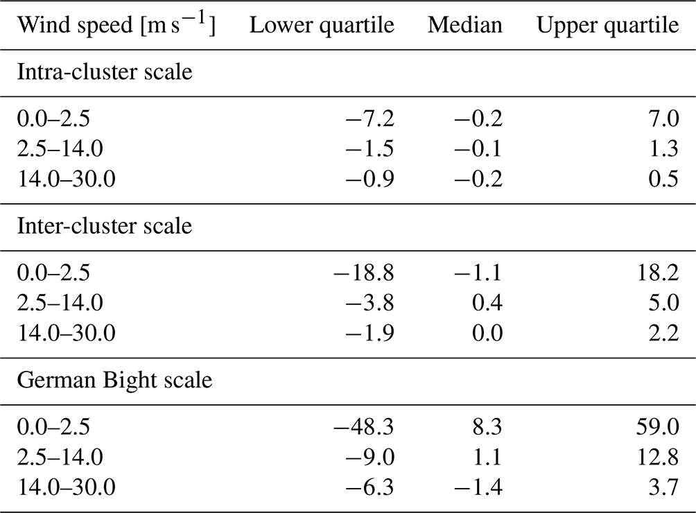
For the different spatial scales, the distances between the locations presented in Fig. 1 are investigated. For the following analysis, we consider different wind speed ranges: below cut-in wind speed (0–2.5 m s−1), the partial load range (2.5–14 m s−1) and above the rated wind speed (>14 m s−1) (Table 1). Those ranges originate from the technical specifications of the different turbine types currently (winter 2022) operational in the German Bight.
Table 1Wind direction changes (in ∘) for the different operational ranges and spatial scales from the NEWA data.
Especially for low wind speeds which are associated with high thrust coefficients, the variability in ΔWD is large while reducing towards higher wind speeds. This is exemplarily shown for the inter-cluster scale as a boxplot in Fig. 4. It can be observed that the median of ΔWD reduces towards the upper partial load range while increasing again towards the cut-out wind speed. Overall, the median varies between about ±1∘. However, in 50 % of the cases as denoted by the quartiles in Fig. 4, considerable wind direction changes of more than 9∘ in the lower operational range (see, e.g., 2.5–5.0 m s−1) can be found. Averaged wind direction changes for the different operational ranges are summarized in Table 1.

Figure 4Wind direction changes between the locations of the wind farms Deutsche Bucht and Global Tech I (distance ≈44 km inter-cluster scale) binned for the wind speed at the reference location (here: FINO1) obtained from 30 years of NEWA data (1989–2018). Green: median; blue box: quartiles; whiskers: 10 % and 90 % percentiles; circles: outliers.
It becomes clear that with increasing distance, the mesoscale direction changes become more relevant. However, also in the intra-cluster scale, 50 % of the cases exceed about 1.5∘ on average in the partial load range. Considering that far-reaching cluster wakes have been measured at distances between the inter-cluster and the German Bight scales, the focus needs to be on these scales concerning cluster wake deflection. Here, wind direction changes are commonly exceeding about 5∘ and about 10∘ in operational conditions, where direction changes reach twice the magnitude in the lower operational wind speed range of 2.5–5.0 m s−1 (not shown). Even though the wake-associated wind speed deficit does not impact the power production above the partial load range, the mechanical loads due to the increased turbulence in the wake can reduce the turbines' lifetime and thus are of relevance.
In the next step, we evaluated the large-scale horizontal patterns of wind direction changes over the 30-year NEWA period (1989–2018) as shown in Fig. 5. The wind direction changes are defined with respect to the reference location FINO1. The wind speed used to bin the results for the median and the quartiles is also derived at the same reference location. The wind direction changes for all wind speeds (see Fig. 5 – upper row) show a dipole pattern for the median, with positive ΔWD on the seaward side of the reference location and negative ones towards the coastal regions. Negative direction changes can be interpreted as clockwise-turning winds (veering), while positive values correspond to counterclockwise-turning winds (backing).

Figure 5Statistics of local wind direction changes with respect to FINO1 for the 30 years of NEWA data and different wind speed ranges. Panels (a, d, g) and (c, f, i) show the lower and upper quartiles, respectively. Panels (b, e, h) show the median for all wind speeds (b) and the wind speed ranges of 2.5–5.0 m s−1 (e) and 12.5–15.0 m s−1 (h). Note the different color scales for the wind speed ranges. The coastline and border data originate from the Natural Earth dataset (Natural Earth, 2021).
Considering the area relevant for offshore wind farms (see Fig. 2), the median of ΔWD ranges between ±5∘. Nevertheless, the upper and lower quartiles show values reaching up to −13 and +10∘ in this offshore region. For the wind speed bin representing the lower partial load range (Fig. 5 – central row), the medians show a similar range, while the quartiles show much larger variation in the data, reaching up to −30 and +25∘. Towards the upper end of the partial load range (Fig. 5 – lower row), this variation reduces to a range of −7 and +5∘. With increasing wind speeds, the dipole pattern of ΔWD becomes more distinct (Fig. 5 – lower row), which aligns well as the main wind direction at FINO1 shifts to the west-southwest for higher wind speeds (see, e.g., Jimenez et al., 2007). This is related to common routes of cyclones over the North Sea (van Bebber, 1891; Hofstätter et al., 2016).
The asymmetry in the wind direction changes is mainly caused by the coastal transition and can thus in particular be observed at the eastern and southern coastlines of the German Bight and for moderate to high wind speeds (see, e.g., Fig. 5). There, comparably large direction changes can reach up to some tens of kilometers offshore. One explanation is the sudden change in surface roughness which leads to a new balance of Coriolis, pressure gradient and frictional forces and thus a turning of the wind direction at the coastline. In the case of sea surface temperatures colder than the advected air mass, an induced stable stratification develops, which can in the end lead to the formation of low-level jets (Emeis, 2018).
Table 2 shows the values of the binned wind direction changes averaged for the selected area (gray area in Fig. 2). It can be summarized that 50 % of all cases show on average a wind direction change of more than 11∘ (first row of Table 2). Focusing on the partial load range (2.5–14 m s−1), the distance between the values of the lower and upper quartiles decrease with increasing wind speed until the upper end of the partial load range. In the lower partial load range, the wind direction changes easily exceed ±20∘ for almost 50 % of the data. Table 2 also reflects that, while the mean wind direction change can be quite low, a large share of situations in particular for wind speeds in the partial load range (<10.0 m s−1) exist with significant wind direction changes. Very high wind speeds, despite being less frequent, come along with larger positive direction changes. One explanation for this could be the passage of cold fronts of low-pressure systems that typically are associated with a strong change in wind direction from southerly to more westerly or even northwesterly winds.
Table 2Values of the percentiles for the wind direction changes (in ∘) with reference to FINO1 for different bins of wind speed at the reference location. The values are calculated as an average of all grid points in the offshore regions of the German Bight (gray area in Fig. 2).

As mentioned, far-reaching cluster wakes were found under both neutral and stable atmospheric stratification. These conditions occur with a probability of 29.2 % at the location of the wind farm Deutsche Bucht, indicated by a positive inverse Obukhov length. Only conditions with wind speeds exceeding 2.5 m s−1 were considered to exclude wind speeds that are below the cut-in wind speed and thus irrelevant for wake formation. Figure 6 shows the magnitude and probability of wind direction changes exceeding the quartiles of −3.2 and +4.2∘ at the inter-cluster scale (DBU and GT I). Conditions under which wind direction changes exceeding the lower and upper quartiles align with atmospheric stratification that benefits far-reaching wakes have a probability of 14.6 %.
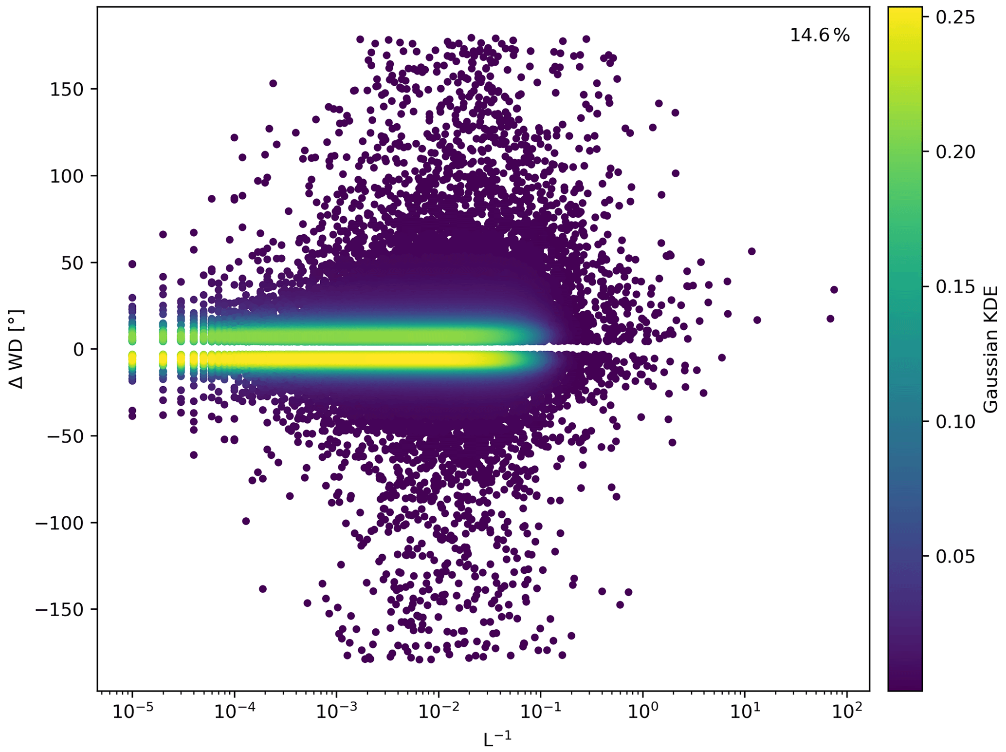
Figure 6Wind direction difference (ΔWD) at the inter-cluster scale (DBU and GT I) for neutral and stable atmospheric stratifications. Only values for wind speeds above 2.5 m s−1 and ΔWD exceeding the lower and upper quartiles are shown, which results in 14.6 % of the data. The color shows a Gaussian kernel density estimation (KDE).
5.1.2 Temporal scale: synoptic pressure systems
To investigate the situation during the passage of synoptic pressure systems over the German Bight, shorter time periods were selected for further investigation.
Figure 7 is a particular example of the wind direction changes happening as the frontal system of Cyclone Sebastian (in September 2017) passed over the German Bight. Typically, low-pressure systems move quite fast from west to east in the northern mid-latitudes, and their frontal systems are associated with strong and sudden wind direction changes. The left plot shows the median of the wind direction changes between each NEWA grid point in the German Bight and the one closest to the reference location FINO1 for a time frame of 48 h around the wind speed maximum.
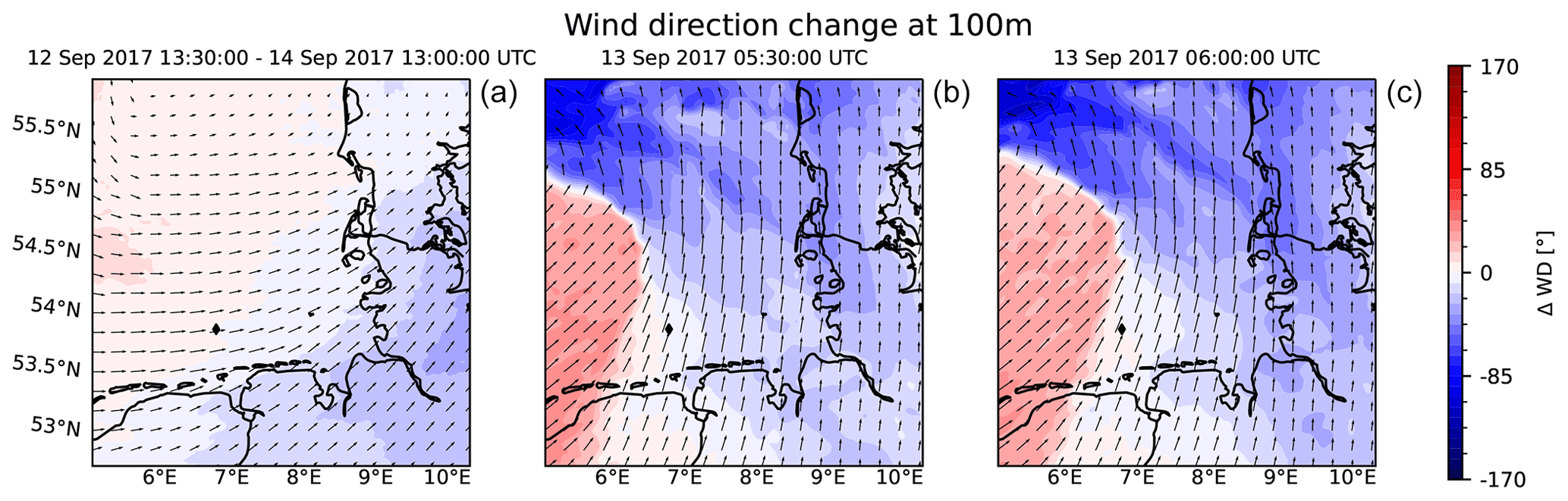
Figure 7Wind direction changes during the passage of Cyclone Sebastian in September 2017. Panel (a) shows the median (time span of 48 h) of the wind direction changes with reference to FINO1, which is marked as a black diamond. Panels (b) and (c) show snapshots of the wind field as the cold front of Sebastian passed over FINO1. The black arrows indicate the wind direction and speed. The coastline and border data originate from the Natural Earth dataset (Natural Earth, 2021).
During the early morning, the cold front passed over the German Bight, causing large wind direction changes (see center and right panels). The comparably large wind direction changes of the instantaneous velocity fields in these panels demonstrate the extent of wind direction changes on shorter timescales. The difference between the mean directions at DBU and GT I for the whole time period from 12 September at 13:30:00 UTC to 14 September 2017 at 13:00:00 UTC is only about 2.3∘, while even smaller values occur for other cyclone passages. Contrasting the small mean difference in wind direction, peaks in ΔWD on the inter-cluster scale were found to reach up to 50 and −80∘ during the passage of the front shown in Fig. 7. This specific situation is further investigated with respect to large-scale wind direction changes in the following sections.
For anticyclones (not shown), comparably large wind direction changes were found for longer time periods. Over the course of 4 d, the difference in mean wind direction at DBU and GT I was, e.g., 6.1∘ (6 May at 00:00:00 UTC to 9 May 2008 at 23:30:00 UTC) and 4.3∘ (25 June at 00:00:00 UTC to 28 June 2018 at 23:30:00 UTC). This highlights that anticyclones can cause wind direction changes at larger scales, persisting over longer time frames.
Specifically, the strong wind direction changes during the passage of cyclones are often less relevant for the power production as the wind speed is mostly above the rated wind speed. Nevertheless, the wake can reduce the wind speed at downstream wind farms to U<Ucut-out. Furthermore, due to the increased turbulence in the wake, these conditions are relevant for load calculation and therefore for the prediction of the turbines' lifetime. Moreover, the warm air advection associated with the frontal system of cyclones influences the atmospheric stability, as it often leads to stable stratification (Bott, 2016; Emeis, 2018) and thus to increased wake lengths.
5.2 Evaluation of the streamline wake model
In this section, the capabilities of the new streamline wake model implemented in flappy are displayed in a series of comparisons. The wake propagation method where every single turbine wake evolves rectilinear downwind, oriented as the wind direction at the wake-causing rotor, is used as the baseline model. For simplicity, in the next paragraphs the new streamline wake model and the baseline model are relabeled with the acronyms SWM and BLM, respectively.
5.2.1 Cluster wake turning associated with synoptic pressure systems
The wake effects of clusters N6 and N8 (see marked clusters in Fig. 2) have been simulated during the passage of the cold front of Cyclone Sebastian (13 September 2017, see Fig. 7).
Figure 8 shows the wind field at about hub height perturbed by the interaction with the wind farms. The three columns display three relevant stages, i.e., instances in time, of the phenomena. The BLM (upper row) shows unexpected wake behavior as soon as the cold front approaches the N6 cluster, with the wakes of the leftmost turbines crossing the ones of the other turbines. When the cold front passes over N6, the wake of this cluster reaches and impacts N8, despite the different wind direction to the right of the front preventing this from happening. In contrast, the lower panels of Fig. 8 show the wakes simulated with the SWM. Already at the first time step, the new model describes the wake propagation in a more sound manner, resolving the wake crossing problem. Also, the following snapshots reveal a more realistic adaptation of the wakes to the heterogeneous background flow.
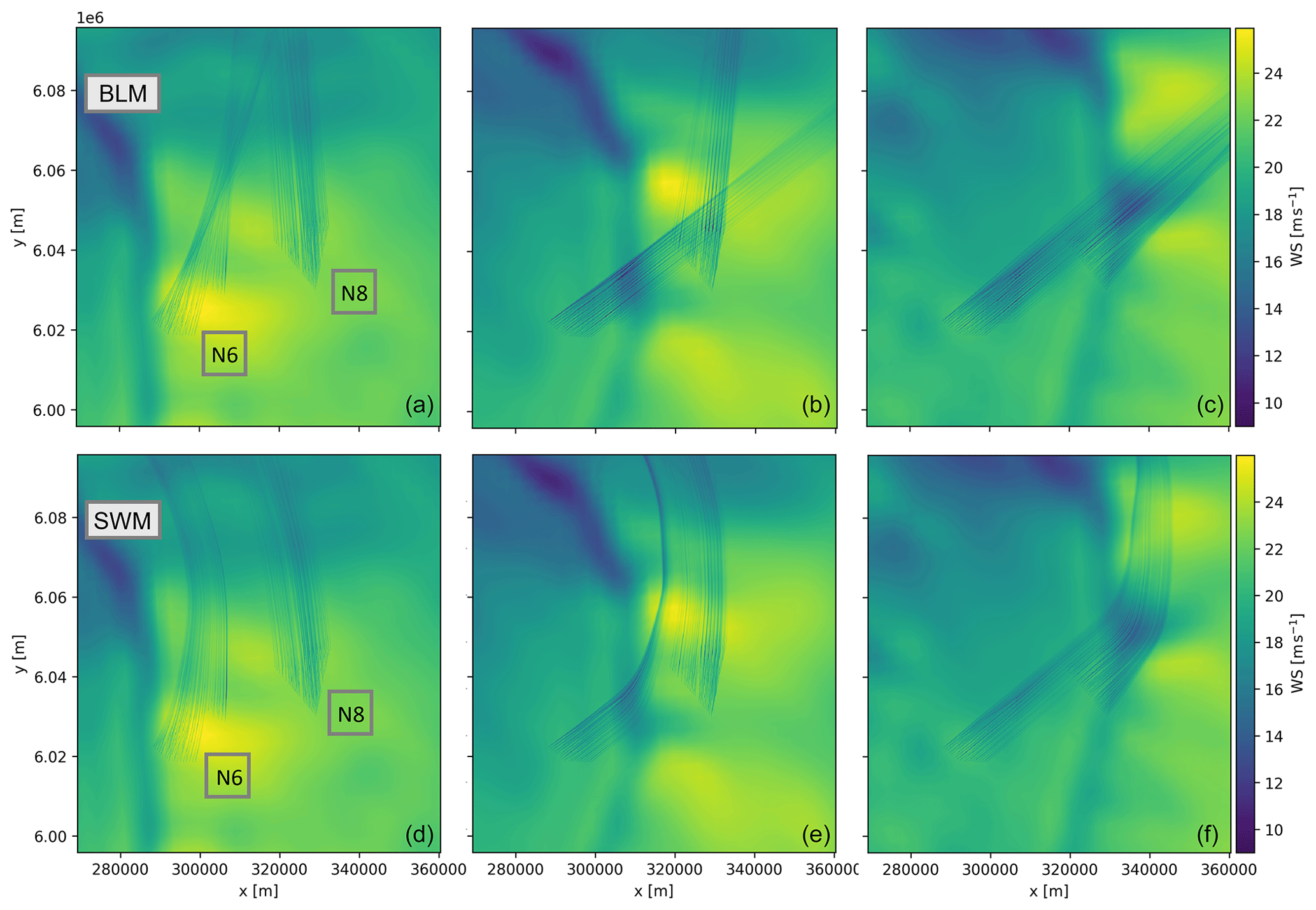
Figure 8Cluster wakes of the N6 and N8 clusters in the German Bight, modeled with the baseline model (a–c) and the new streamline wake model (d–f). The situation chosen is the passage of a cold front captured in the mesoscale data of the NEWA on 13 September 2017. The wind speed [m s−1] at hub height is shown from left to right for the following times: 05:00:00, 05:30:00 and 06:00:00 UTC. The coordinates are given in UTM format (Zone 32U) with meters easting on the x axis and meters northing on the y axis.
5.2.2 Qualitative comparison to SAR images
To demonstrate that the SWM calculates the trajectory along which cluster wakes evolve with greater fidelity than the BLM, few comparisons to SAR imagery were performed. Here, only a single situation considered in the comparison is depicted in Fig. 9. The lower panel shows the normalized radar cross-section (NRCS) from Sentinel-1A, acquired at 05:48 UTC. In the eastward direction, the shadow areas and streaks downstream of the wind farms indicate low backscatter and correspond to the region of reduced wind speed that characterized the wakes. Quite long wakes and an evident wake turning induced by westerly winds that get a more northern component in the southern part of the German Bight are visible. The upper panels of Fig. 9 show the wind speed at hub height above the mean sea level in the German Bight simulated for 21 March 2018 at 06:30:00 UTC. All wind farms installed in the area on that date have been considered. However, precise information on the turbine operation states was missing. In this situation, the underlying WRF data suggest a westerly wind that is not particularly strong. Thus, the turbines operate at maximum thrust, offering long persisting wakes. Furthermore, as the focus in the comparison is the wake trajectories, the wake model coefficients are chosen so as to minimize wake recovery and show the wake evolution throughout the domain. The results of the simulations with the BLM (upper left panel) differ significantly from the one of the SWM (upper right panel). In comparison to the SAR image (bottom panel), the SWM captures with higher fidelity the trajectory of the cluster wakes of the southern clusters, allowing us to correctly represent the distinct anticyclonic turning of the N3 cluster wake. Also, when looking at the Gemini cluster, we observe a much better agreement of the model with SAR when the SWM is used instead of the BLM.
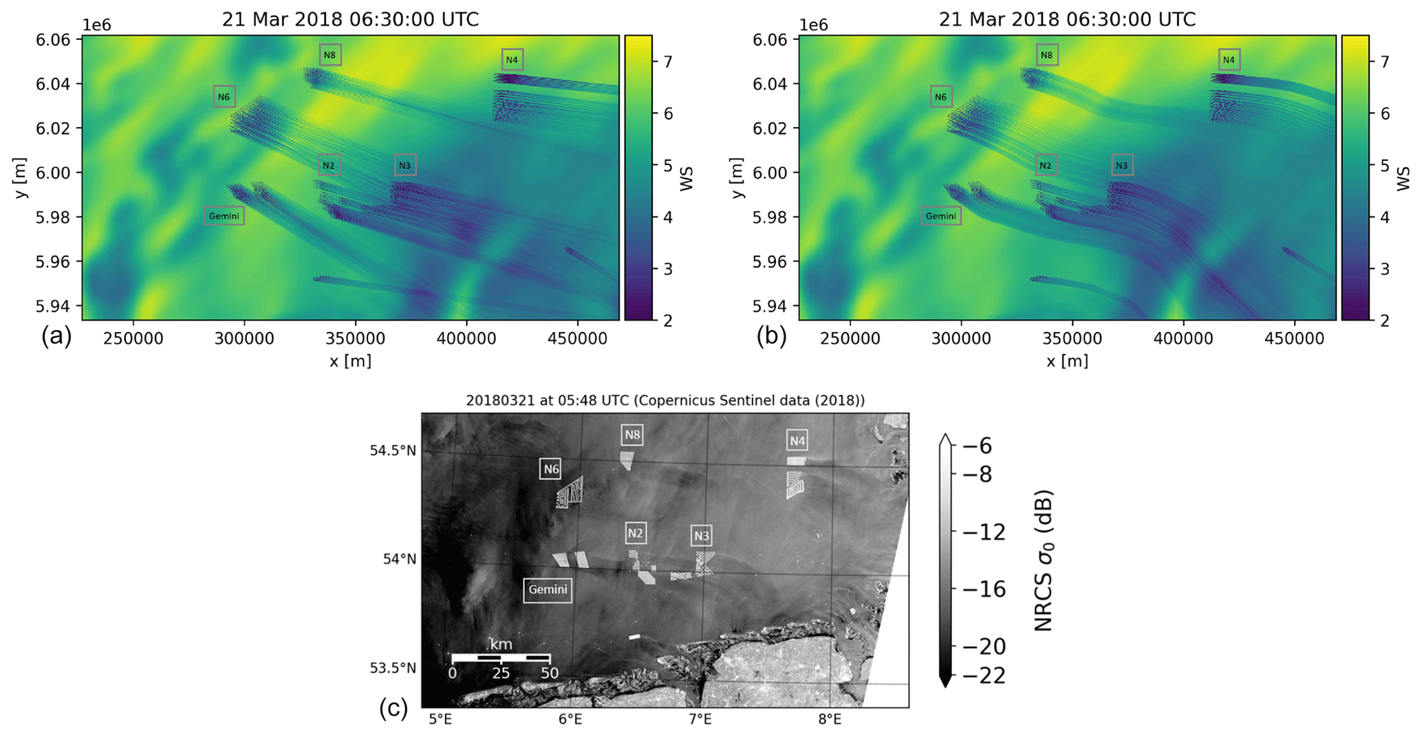
Figure 9(a, b) Wind speed [m s−1] at hub height in the German Bight for 21 March 2018 at 06:30:00 UTC, simulated with flappy for all wind farms commissioned to that date. (a) Baseline model with straight wake propagation and (b) the new streamline wake model. (c) SAR image from Copernicus Sentinel data (ESA 2000–2020) showing cluster wakes in the German Bight on 21 March 2018 at 05:48:00 UTC. The white dots show the wind turbines and the shading the backscatter value σ0 of the normalized radar cross-section (NRCS).
Note that the displayed SAR was taken about 45 min earlier than the mesoscale model data. The different time in the models was chosen as it provided the best agreement with the SAR data, acknowledging that phase errors up to several hours are a well-known phenomenon in mesoscale model data.
The SWM agreed well with the SAR data in only a few other situations considered; however, we observe cases where the agreement between SAR and both models was poor (not shown). For these cases, the mismatch is mostly related to a fundamental disagreement between SAR and the WRF mesoscale data used as input of the engineering models. While Dörenkämper et al. (2020) found that on average the mesoscale atlas of the NEWA represents offshore wind conditions well, the generated wind fields may present local errors. Recently, the NEWA atlas has been subject to validation activities for different applications (e.g., Hallgren et al., 2020; Kalverla et al., 2020; Luzia et al., 2022). At the same time, SAR imagery has not been demonstrated yet as a reliable tool for quantitative wake model validation, as the data acquired have uncertainty of up to 2 m s−1 (Hasager et al., 2020). In conclusion, the comparison of Fig. 9 cannot be considered a validation of the new method, but it highlighted that in no case was the wakes' directional propagation computed by the BLM superior to the SWM.
5.2.3 Impact on energy yield assessment
In this section, we discuss the differences across the SWM and BLM when applied to computing the energy yield at two wind farm clusters impacting each other. Assuming the proposed method as an improvement over the common BLM, these simulations provide an estimate of the new model's potential to partly reduce and especially understand the sources of uncertainty in engineering wake model applications.
As before, the selected clusters for the study are clusters N6 and N8 in the German Bight. The tool flappy is applied for calculating the power production at any time step in the last 10 years of the NEWA mesoscale data with the BLM and the SWM.
As a first analysis, the total energy yield of N6 and N8 when operating together is calculated. The simulation setup adopted is described in detail in Sect. 3.2. In addition to the two wake propagation methods, also two different superposition methods for the velocity deficit will be considered. Table 3 briefly summarizes the four simulations performed for this analysis.
Table 3Simulations performed with the two wake propagation models and two wake superposition models in flappy.

The energy yield simulated over a period of 10 years shows that the SWM results are very similar to the BLM results. The relative difference in the yield of both clusters is 0.01 % and 0.004 % for the superposition models' wind product and wind linear, respectively. However, the differences in the calculation for single situations are significantly greater, as demonstrated by the standard deviation found to be 1.21 % and 1.05 % for wind product and wind linear, respectively. Thus, BLM and SWM would compute differently the energy production when considering shorter time frames.
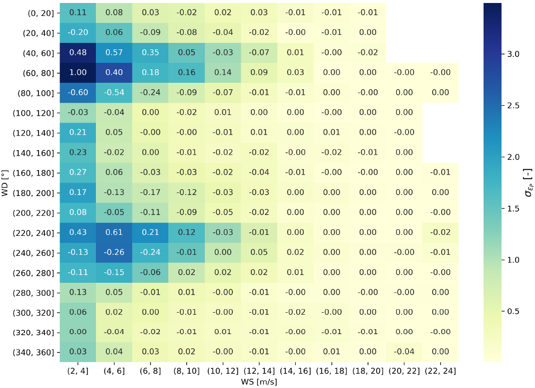
Most interestingly, the largest differences happen systematically according to wind direction and wind speed, as demonstrated in the heatmap of Table 4. According to the color coding, the relative difference between the models is greater for very low wind speeds or for wind speeds in the partial load range and wind directions where the clusters align. This can be explained by effects on the intra-cluster and the inter-cluster scales. As already discussed in Sect. 5.1, very low wind speeds are often associated with very inhomogeneous wind fields. Therefore, significant wind direction changes are observed even at an intra-cluster scale. In this case, the models can provide different results even in situations where the two clusters should not interact through their wakes due to differing wake propagation within one cluster. For higher wind speeds, the differences between the models are grouped around the wind directions along which the clusters align. Once the wind speed exceeds the rated speed, the differences progressively reduce as pitching control reduces the intensity of the wakes. Looking at the mean relative difference between the models, the SWM predicts a larger energy production in all the occasions where the main wind direction is such that the clusters align: bins [40, 60]–[60, 80], [220–240]. This is coherent with the fact that accounting for wake turning, the waked cluster will produce more, experiencing more “free-stream” velocity. At the same time, the SWM computes a lower yield than the BLM when the wind direction has an offset. A trend of counterclockwise turning in the wake is highlighted by the fact that the SWM computes the lowest yield with respect to the BLM for the bins [80, 100], [240, 260].
Table 4Heatmap of the standard deviation (colors) and mean (annotated number) of the relative difference between the streamline wake model and the baseline model in the calculation of the energy yield of the N6 and N8 cluster. Here, the wind linear superposition was applied. The mean and the standard deviation are computed as and , respectively, with n the last time step of the NEWA time series considered. The wind speed and direction considered for the bin are taken from the easternmost turbine row of cluster N6.
The results presented so far suggest that the use of the SWM could be useful for two main practices that engineering models enable: site assessment for new wind farms and short-term forecasting for, e.g., a grid following control strategies. In both applications, it is important to guarantee that the engineering models compute with a sufficient level of accuracy on short timescales.
The quantitative differences discussed so far are comprised of differences in the wake development, both on the scale of a single farm and the cluster wake scale. However, the underlying mesoscale data represent the flow field at the scale of cluster wakes well while lacking the accuracy to correctly describe the wind direction changes at a scale of a few rotor diameters. Thus, the uncertainty introduced by the effects within a cluster is isolated by performing the same set of simulations (C1–4; Table 3) for N8 without N6. In these simulations, the energy yield of N8 is only affected by the intra-cluster effects. Therefore, the difference in energy yield of only N8 between these and the previous simulations gains the yield loss due to the cluster wake of N6. This value is again compared across the SWM and BLM to estimate how the new model offers a different prediction of cluster wake effects between neighboring clusters. The resulting differences for the two wake superposition models' wind linear and wind product are 0.5 % and 0.7 %, respectively.
In conclusion, in our results, the proposed model offers a small but non-negligible difference when estimating the interaction between neighboring wind farm clusters, like N6 and N8. Despite the new model not yet being validated with production data, we speculate that such a difference could represent an actual improvement over the baseline in terms of model accuracy.
Finally, it may be worth remembering that the applied wake model, optimized on a single wind farm, is likely underestimating the extent of cluster wakes. This aspect, in addition to the fact that a new wind farm cluster will most likely be surrounded by more than just one, could easily increase the gap between the BLM and the SWM, making the second more attractive.
5.3 Limitations of the streamline wake model
Several assumptions were made in the construction of the proposed streamline wake model, as in the context of engineering modeling any accuracy improvement should not compromise computational speed.
The major assumption is that the wakes propagate according to the streamlines rather than being a Lagrangian tracer. This means that any time step of the NEWA time series is considered a stationary flow field that lasts for a sufficiently long time to allow the wake to propagate to its maximum extent. This assumption mainly stems from the coarse temporal resolution of the mesoscale data of 30 min that would hinder the application of a true wake advection algorithm. However, due to this simplification all the various states remain independent of each other, allowing for a simplified algorithm and a more efficient parallelization.
A further assumption taken is that the wakes cannot modify the background wind field, and thus the wake deficit is designed to always be aligned to the local background wind vector. Mostly in complex wind fields with convective behavior or strong shear, this yields an unknown uncertainty. However, there are no sufficient studies of wakes in such situations to choose a more sophisticated approach.
Further simplifications concern both the horizontal and the vertical description of the wake. As explained by van der Laan and Sørensen (2017) the direction in which a turbine wake propagates is influenced by both the wind veer and the Coriolis force. The wake modifies the vertical wind velocity profile, unbalancing the local equilibrium of forces. As a result, the wind direction is locally changed in agreement with the Coriolis force. At the same time, the additional shear introduced by the wake deficit promotes mixing, especially from above. Due to this phenomenon, the local wind direction is also affected by the entrainment of the fluid layers above the wake that have a different wind direction due to the Ekman spiral. Gadde and Stevens (2019) found that the propagation of the wake of a wind farm in a homogeneous inflow is determined only by the entrainment of wind veer, and the effect of the Coriolis force is almost negligible. However, both of these phenomena are neglected in the computation of the wake trajectory with the SWM. Considering such local phenomena is expected to lead to a small gain in accuracy compared to the large uncertainty of mesoscale data in characterizing the flow at the turbine level. Additionally, the iterative calculation of the streamlines which would be necessary to include such effects would increase the calculation time.
Mesoscale wind direction changes are found to exceed 11∘ in 50 % of all cases, referring to mesoscale data simulated in the NEWA from 1989 to 2018, averaged for the German Bight. Particularly for wind speeds in the lower partial load range, large wind direction changes occur, with the quartiles reaching up to 20∘. Wind direction changes are found to be specifically relevant on the horizontal scale of several tens of kilometers to 100 km. Synoptic pressure systems were found to lead to large wind direction changes which persist over shorter time periods for low-pressure systems and longer time periods for synoptic high-pressure systems. Also, the evidence of coastal effects can be found in the wind direction changes to some tens of kilometers offshore. Moreover, atmospheric conditions promoting far-reaching wind farm wakes were found to coexist with larger wind direction changes between wind farm clusters in 14.6 % of the cases. This favors the occurrence of far-reaching wakes with a strong turning on the scale of cluster to cluster interactions.
The magnitude and frequency of the wind direction changes observed in the mesoscale suggest that the uncertainty in the modeling of wind farms, especially for engineering models, can rise significantly with the number of farms simulated if the wake propagation disregards changes in the flow direction. Thus, we present a new framework for engineering models that, given a 3D-resolved wind field as input, accounts for wake turning with the background flow. This is realized by assuming the single turbine wake centerline evolves as the streamline starting at the location of the wake-causing turbine in the 2D horizontal flow field located at hub height. Initial qualitative and quantitative results obtained through the method implementation in the Fraunhofer IWES wind farm modeling tool flappy are also discussed.
A qualitative comparison of the simulated flow fields around the wind farm clusters in the German Bight with SAR data shows that the new model can represent the flow in a way more consistent to physics than the common baseline approach. We conclude that the ability of the model to represent large-scale direction changes depends greatly on the accuracy of the underlying data (NEWA data in the discussed cases) in representing those. However, in no occasion did the BLM provide a better representation of the wake propagation than the SWM.
In our quantitative studies, the new streamline wake model brought little to no benefit over the baseline when focusing on computing the energy yield of multiple wind farms across several years. However, considering more than two wind farm clusters and a wake model tuning favoring an accurate description of the cluster wakes, it is likely to obtain a different result. On the other hand, significant differences between the models are observed when computing the power output on shorter time frames or the impact of surrounding clusters on a site of interest. Despite no validation being possible, given the positive feedback provided by the qualitative comparison to SAR, we believe that the proposed method could offer higher accuracy in how the engineering model computes wind farms' performances in single situations or shorter time frames. Therefore, as the coupling of engineering models and mesoscale data could change the paradigm of site assessment and offer the possibility of grid following control strategies on a multi-wind-farm logic, we recommend the proposed model for these purposes.
Future development, partly already initiated, encompasses the attempt of validating the model with a combination of lidar measurements and wind farm production data, as well as the comparison to other large-scale cluster wake modeling approaches such as mesoscale wake modeling (Fischereit et al., 2022a). The study by Fischereit et al. (2022b) provides an attempt of comparing different wake models of different complexity, although on a smaller scale than the German Bight. This validation should then also focus on the validity of the assumption of stationarity of the streamlines.
The modeling results in this paper were obtained using the Fraunhofer IWES in-house code flappy, which has recently been released as open-source software under the new name FOXES – Farm Optimization and eXtended yield Evaluation Software via https://doi.org/10.5281/zenodo.7852145 (Schmidt, 2023). The mesoscale data used for computing the streamlines originate from the New European Wind Atlas which is publicly available via https://map.neweuropeanwindatlas.eu/ (NEWA, 2023).
AvB did most of the data curation and analysis and suggested the first version of a deflection mechanism. She drafted a first version of the manuscript. AvB, GC and JS implemented the wake deflection model. JS is the key developer of the flappy model. LV was involved in the derivation of the model setup and the calibration of the wake model. BD was mainly involved in the discussion of the SAR validation. MD initiated the research, supervised the work, and was mainly involved in the funding acquisition and the research discussion. All authors contributed intensively to the writing and review of the manuscript.
The contact author has declared that none of the authors has any competing interests.
Publisher's note: Copernicus Publications remains neutral with regard to jurisdictional claims in published maps and institutional affiliations.
We thank the NEWA consortium for making the mesoscale data set available to the public. Maps have been generated using the cartopy (Met Office, 2010–2015) library for Python.
The results presented in this paper were derived in the framework of the X-Wakes (grant no. 03EE3008) project. The X-Wakes project is funded by the German Federal Ministry for Economic Affairs and Climate Action (Bundesministerium für Wirtschaft und Klimaschutz – BMWK) due to a decision of the German Bundestag. The simulations were partly performed at the HPC Cluster EDDY, located at the University of Oldenburg (Germany) funded by BMWK (grant no. 0324005).
This paper was edited by Johan Meyers and reviewed by two anonymous referees.
Agora Energiewende: Making the Most of Offshore Wind: Re-Evaluating the Potential of Offshore Wind in the German North Sea. Re-Evaluating the Potential of Offshore Wind in the German North Sea, Tech. Rep. 176/01-S-2020/EN 36-2020-EN, Agora Energiewende, Agora Verkehrswende, Technical University of Denmark and Max-Planck-Institute for Biogeochemistry, https://static.agora-energiewende.de/fileadmin/Projekte/2019/Offshore_Potentials/176_A-EW_A-VW_Offshore-Potentials_Publication_WEB.pdf (last access: 11 April 2023), 2020. a
Ahsbahs, T., Nygaard, N. G., Newcombe, A., and Badger, M.: Wind Farm Wakes from SAR and Doppler Radar, Remote Sens., 12, 462, https://doi.org/10.3390/rs12030462, 2020. a, b
Bastankhah, M. and Porté-Agel, F.: Experimental and theoretical study of wind turbine wakes in yawed conditions, J. Fluid Mech., 806, 506–541, https://doi.org/10.1017/jfm.2016.595, 2016. a
Bott, A.: Synoptische Meteorologie, Springer, Berlin, Heidelberg, https://doi.org/10.1007/978-3-662-48195-0, 2016. a, b
Bundesamt für Seeschifffahrt und Hydrographie: Shape Files of the extensions of the existing wind farms in the German Bight, CONTIS Facilities, https://www.geoseaportal.de/mapapps/?lang=en, last access: 26 November 2020. a, b
Cañadillas, B., Foreman, R., Barth, V., Siedersleben, S. K., Lampert, A., Platis, A., Djath, B., Schulz-Stellenfleth, J., Bange, J., Emeis, S., and Neumann, T.: Offshore wind farm wake recovery: Airborne measurements and its representation in engineering models, Wind Energy, 23, 1249–1265, https://doi.org/10.1002/we.2484, 2020. a, b, c
Cañadillas, B., Beckenbauer, M., Trujillo, J. J., Dörenkämper, M., Foreman, R., Neumann, T., and Lampert, A.: Offshore wind farm cluster wakes as observed by long-range-scanning wind lidar measurements and mesoscale modeling, Wind Energ. Sci., 7, 1241–1262, https://doi.org/10.5194/wes-7-1241-2022, 2022. a
Centurelli, G., Vollmer, L., Schmidt, J., Dörenkämper, M., Schröder, M., Lukassen, L., and Peinke, J.: Evaluating Global Blockage engineering parametrizations with LES, J. Phys.: Conf. Ser., 1934, 012021, https://doi.org/10.1088/1742-6596/1934/1/012021, 2021. a
Christiansen, M. B. and Hasager, C. B.: Wake effects of large offshore wind farms identified from satellite SAR, Remote Sens. Environ., 98, 251–268, https://doi.org/10.1016/j.rse.2005.07.009, 2005. a
Crespo, A., Hernández, J., and Frandsen, S.: Survey of modelling methods for wind turbine wakes and wind farms, Wind Energy, 2, 1–24, https://doi.org/10.1002/(sici)1099-1824(199901/03)2:1<1::aid-we16>3.3.co;2-z, 1999. a
Djath, B. and Schulz-Stellenfleth, J.: Wind speed deficits downstream offshore wind parks – A new automised estimation technique based on satellite synthetic aperture radar data, Meteorol. Z., 28, 499–515, https://doi.org/10.1127/metz/2019/0992, 2019. a
Djath, B., Schulz-Stellenfleth, J., and Cañadillas, B.: Impact of atmospheric stability on X-band and C-band synthetic aperture radar imagery of offshore windpark wakes, J. Renew. Sustain. Energ., 10, 043301, https://doi.org/10.1063/1.5020437, 2018. a, b
Dörenkämper, M., Olsen, B. T., Witha, B., Hahmann, A. N., Davis, N. N., Barcons, J., Ezber, Y., García-Bustamante, E., González-Rouco, J. F., Navarro, J., Sastre-Marugán, M., Sīle, T., Trei, W., Žagar, M., Badger, J., Gottschall, J., Sanz Rodrigo, J., and Mann, J.: The Making of the New European Wind Atlas – Part 2: Production and Evaluation, Geosci. Model Dev., 13, 5079–5102, https://doi.org/10.5194/gmd-13-5079-2020, 2020. a, b
Emeis, S.: A simple analytical wind park model considering atmospheric stability, Wind Energy, 13, 459–469, https://doi.org/10.1002/we.367, 2010. a
Emeis, S.: Wind Energy Meteorology: Atmospheric Physics for Wind Power Generation, in: 2nd Edn., Springer International Publishing, Cham, Switzerland, https://doi.org/10.1007/978-3-319-72859-9, 2018. a, b, c
Eriksson, O., Breton, S.-P., Nilsson, K., and Ivanell, S.: Impact of Wind Veer and the Coriolis Force for an Idealized Farm to Farm Interaction Case, Appl. Sci., 9, 922, https://doi.org/10.3390/app9050922, 2019. a, b
European Commission: Communication from the commission to the European Parliament, the European Council, the European Economic and Social Committee and the Committee of the Regions - The European Green Deal, Technical report, European Commission, 24 pp., https://eur-lex.europa.eu/resource.html?uri=cellar:b828d165-1c22-11ea-8c1f-01aa75ed71a1.0002.02/DOC_1&format=PDF (last access: 24 December 2021), 2019. a
Farrell, A., King, J., Draxl, C., Mudafort, R., Hamilton, N., Bay, C. J., Fleming, P., and Simley, E.: Design and analysis of a wake model for spatially heterogeneous flow, Wind Energ. Sci., 6, 737–758, https://doi.org/10.5194/wes-6-737-2021, 2021. a
Fischereit, J., Brown, R., Larsén, X. G., Badger, J., and Hawkes, G.: Review of Mesoscale Wind-Farm Parametrizations and Their Applications, Bound.-Lay. Meteorol., 182, 175–224, https://doi.org/10.1007/s10546-021-00652-y, 2022a. a
Fischereit, J., Schaldemose Hansen, K., Larsén, X. G., van der Laan, M. P., Réthoré, P.-E., and Murcia Leon, J. P.: Comparing and validating intra-farm and farm-to-farm wakes across different mesoscale and high-resolution wake models, Wind Energ. Sci., 7, 1069–1091, https://doi.org/10.5194/wes-7-1069-2022, 2022b. a
Gadde, S. N. and Stevens, R. J.: Effect of Coriolis force on a wind farm wake, J. Phys.: Conf. Ser., 1256, 012026, https://doi.org/10.1088/1742-6596/1256/1/012026, 2019. a, b, c
Hahmann, A. N., Sīle, T., Witha, B., Davis, N. N., Dörenkämper, M., Ezber, Y., García-Bustamante, E., González-Rouco, J. F., Navarro, J., Olsen, B. T., and Söderberg, S.: The making of the New European Wind Atlas – Part 1: Model sensitivity, Geosci. Model Dev., 13, 5053–5078, https://doi.org/10.5194/gmd-13-5053-2020, 2020. a
Hallgren, C., Arnqvist, J., Ivanell, S., Körnich, H., Vakkari, V., and Sahlée, E.: Looking for an offshore low-level jet champion among recent reanalyses: a tight race over the Baltic Sea, Energies, 13, 3670, doi10.3390/en13143670, 2020. a
Hasager, C. B., Madsen, P. H., Giebel, G., Réthoré, P.-E., Hansen, K. S., Badger, J., Peña, A., Volker, P., Badger, M., Karagali, I., Cutulusis, N., Maule, P., Schepers, G., Wiggelinkhuizen, E. J., Cantero, E., Waldl, I., Anaya-Lara, O., Attya, A. B., Svendsen, H., Palomares, A., Palma, J., Gomes, V. C., Gottschall, J., Wolken-Möhlmann, G., Bastigkeit, I., Beck, H., Trujillo, J. J., Barthelmie, R., Sieros, G., Chaviaropoulos, T., Vincent, P., Husson, R., and Propathopoulos, J.: Design tool for offshore wind farm cluster planning, in: Proceedings of the EWEA Annual Event and Exhibition, Paris, France, https://orbit.dtu.dk/en/publications/design-tool-for-offshore-wind-farm-cluster-planning (last access: 20 April 2023), 2015a. a
Hasager, C. B., Vincent, P., Badger, J., Badger, M., Di Bella, A., Peña, A., Husson, R., and Volker, P.: Using Satellite SAR to Characterize the Wind Flow around Offshore Wind Farms, Energies, 8, 5413–5439, https://doi.org/10.3390/en8065413, 2015b. a
Hasager, C. B., Hahmann, A. N., Ahsbahs, T., Karagali, I., Sīle, T., Badger, M., and Mann, J.: Europe's offshore winds assessed with synthetic aperture radar, ASCAT and WRF, Wind Energ. Sci., 5, 375–390, https://doi.org/10.5194/wes-5-375-2020, 2020. a
Hersbach, H., Stoffelen, A., and de Haan, S.: An improved C-band scatterometer ocean geophysical model function: CMOD5, J. Geophys. Res., 112, C03006, https://doi.org/10.1029/2006JC003743, 2007. a
Hofstätter, M., Chimani, B., Lexer, A., and Blöschl, G.: A new classification scheme of European cyclone tracks with relevance to precipitation, Water Resour. Res., 52, 7086–7104, https://doi.org/10.1002/2016WR019146, 2016. a
Jacobsen, S., Lehner, S., Hieronimus, J., Schneemann, J., and Kühn, M.: Joint Offshore Wind Field Monitoring with Spaceborne SAR and Platform-Based Doppler LiDAR Measurements, Int. Arch. Photogramm. Remote Sens. Spat. Inf. Sci.-ISPRS Arch., XL-7/W3, 959–966, https://doi.org/10.5194/isprsarchives-XL-7-W3-959-2015, 2015. a
Jimenez, B., Durante, F., Lange, B., Kreutzer, T., and Tambke, J.: Offshore wind resource assessment with WAsP and MM5: comparative study for the German Bight, Wind Energy, 10, 121–134, https://doi.org/10.1002/we.212, 2007. a
Kalverla, P. C., Holtslag, A. A., Ronda, R. J., and Steeneveld, G.-J.: Quality of wind characteristics in recent wind atlases over the North Sea, Q. J. Roy. Meteorol. Soc., 146, 1498–1515, https://doi.org/10.1002/qj.3748, 2020. a
Lanzilao, L. and Meyers, J.: A new wake-merging method for wind-farm power prediction in presence of heterogeneous background velocity fields, http://arxiv.org/pdf/2010.03873v1 (last access: 9 February 2022), 2020. a, b
Lanzilao, L. and Meyers, J.: A new wake-merging method for wind-farm power prediction in the presence of heterogeneous background velocity fields, Wind Energy, 25, 237–259, https://doi.org/10.1002/we.2669, 2022. a, b
Li, X. and Lehner, S.: Observation of TerraSAR-X for Studies on Offshore Wind Turbine Wake in Near and Far Fields, IEEE J. Select. Top. Appl. Earth Obs. Remote Sens., 6, 1757–1768, https://doi.org/10.1109/JSTARS.2013.2263577, 2013. a
Luzia, G., Hahmann, A. N., and Koivisto, M. J.: Evaluating the mesoscale spatio-temporal variability in simulated wind speed time series over northern Europe, Wind Energ. Sci., 7, 2255–2270, https://doi.org/10.5194/wes-7-2255-2022, 2022. a
Machefaux, E., Larsen, G. C., and Leon, J. P. M.: Engineering models for merging wakes in wind farm optimization applications, J. Phys.: Conf. Ser., 625, 012037, https://doi.org/10.1088/1742-6596/625/1/012037, 2015. a
Met Office: Cartopy: a cartographic python library with a matplotlib interface, Exeter, Devon, http://scitools.org.uk/cartopy (last access: 1 November 2021), 2010–2015. a
Natural Earth: Free vector and raster map data, https://www.naturalearthdata.com/, last access: 1 November 2021. a, b, c, d
NEWA: New European Wind Atlas Website and Database, https://map.neweuropeanwindatlas.eu/, last access: 21 April 2023. a
Niayifar, A. and Porté-Agel, F.: A new analytical model for wind farm power prediction, J. Phys.: Conf. Ser., 625, 012039, https://doi.org/10.1088/1742-6596/625/1/012039, 2015. a
NREL: FLORIS. Version 2.2.0, https://github.com/NREL/floris (last access: 1 November 2021), 2020. a
Nygaard, N. G. and Hansen, S. D.: Wake effects between two neighbouring wind farms, J. Phys.: Conf. Ser., 753, 032020, https://doi.org/10.1088/1742-6596/753/3/032020, 2016. a
Nygaard, N. G., Steen, S. T., Poulsen, L., and Pedersen, J. G.: Modelling cluster wakes and wind farm blockage, J. Phys.: Conf. Ser., 1618, 062072, https://doi.org/10.1088/1742-6596/1618/6/062072, 2020. a
Peña, A. and Rathmann, O.: Atmospheric stability-dependent infinite wind-farm models and the wake-decay coefficient, Wind Energy, 17, 1269–1285, https://doi.org/10.1002/we.1632, 2014. a
Platis, A., Siedersleben, S. K., Bange, J., Lampert, A., Bärfuss, K., Hankers, R., Cañadillas, B., Foreman, R., Schulz-Stellenfleth, J., Djath, B., Neumann, T., and Emeis, S.: First in situ evidence of wakes in the far field behind offshore wind farms, Sci. Rep., 8, 2163, https://doi.org/10.1038/s41598-018-20389-y, 2018. a, b, c, d
Platis, A., Bange, J., Bärfuss, K., Cañadillas, B., Hundhausen, M., Djath, B., Lampert, A., Schulz-Stellenfleth, J., Siedersleben, S., Neumann, T., and Emeis, S.: Long-range modifications of the wind field by offshore wind parks – results of the project WIPAFF, Meteorol. Z., 29, 355–376, https://doi.org/10.1127/metz/2020/1023, 2020. a
Portabella, M.: Toward an optimal inversion method for synthetic aperture radar wind retrieval, J. Geophys. Res., 107, 3086, https://doi.org/10.1029/2001JC000925, 2002. a
Schmidt, J.: Farm Optimization and eXtended yield Evaluation Software (v0.3.4-doi), Zenodo [code], https://doi.org/10.5281/zenodo.7852145, 2023. a, b
Schmidt, J. and Stoevesandt, B.: Wind farm layout optimisation using wakes from computational fluid dynamics simulations, in: EWEA conference proceedings, 10–13 March 2014, Barcelona, Spain, https://doi.org/10.13140/2.1.2544.3847, 2014. a
Schmidt, J. and Stoevesandt, B.: Wind farm layout optimisation in complex terrain with CFD wakes, in: EWEA conference proceedings, 17–20 November 2015, Paris, France, https://www.ewea.org/annual2015/conference/submit-an-abstract/pdf/287736207932.pdf (last access: 20 April 2023), 2015. a
Schmidt, J. and Vollmer, L.: Industrial Wake Models, in: Handbook of Wind Energy Aerodynamics, edited by: Stoevesandt, B., Schepers, G., Fuglsang, P., and Yuping, S., Springer International Publishing, Cham, 1–28, https://doi.org/10.1007/978-3-030-05455-7_49-1, 2020. a
Schmidt, J., Requate, N., and Vollmer, L.: Wind Farm Yield and Lifetime Optimization by Smart Steering of Wakes, J. Phys.: Conf. Ser., 1934, 012020, https://doi.org/10.1088/1742-6596/1934/1/012020, 2021. a
Schmidt, J., Requate, N., Vollmer, L., and Meyer, T.: Adaptive time-series based wind farm optimization, in: Wind Energy Science Conference 2021, 25–28 May 2021, Hannover, Germany, 2022. a
Schneemann, J., Hieronimus, J., Jacobsen, S., Lehner, S., and Kühn, M.: Offshore wind farm flow measured by complementary remote sensing techniques: radar satellite TerraSAR-X and lidar windscanners, J. Phys.: Conf. Ser., 625, 012015, https://doi.org/10.1088/1742-6596/625/1/012015, 2015. a
Schneemann, J., Rott, A., Dörenkämper, M., Steinfeld, G., and Kühn, M.: Cluster wakes impact on a far-distant offshore wind farm's power, Wind Energ. Sci., 5, 29–49, https://doi.org/10.5194/wes-5-29-2020, 2020. a, b, c, d, e
Siedersleben, S. K., Platis, A., Lundquist, J. K., Lampert, A., Bärfuss, K., Cañadillas, B., Djath, B., Schulz-Stellenfleth, J., Bange, J., Neumann, T., and Emeis, S.: Evaluation of a Wind Farm Parametrization for Mesoscale Atmospheric Flow Models with Aircraft Measurements, Meteorol. Z., 27, 401–415, https://doi.org/10.1127/metz/2018/0900, 2018. a
SPD, Bündnis 90/Die Grünen, and FDP: Mehr Fortschritt wagen, Bündnis für Freiheit, Gerechtigkeit und Nachhaltigkeit – Koalitionsvertrag zwischen SPD, Bündnis 90/Die Grünen und FDP, https://www.bundesregierung.de/breg-de/service/gesetzesvorhaben/koalitionsvertrag-2021-1990800 (last access: 27 January 2022), 2021. a
van Bebber, W. J.: Die Zugstrassen der barometrischen Minima, Meteorol. Z., 8, 361–366, 1891. a
van der Laan, M. P. and Sørensen, N. N.: Why the Coriolis force turns a wind farm wake clockwise in the Northern Hemisphere, Wind Energy Science, 2, 285–294, https://doi.org/10.5194/wes-2-285-2017, 2017. a, b
van der Laan, M. P., Hansen, K. S., Sørensen, N. N., and Réthoré, P.-E.: Predicting wind farm wake interaction with RANS: an investigation of the Coriolis force, J. Phys.: Conf. Ser., 625, 012026, https://doi.org/10.1088/1742-6596/625/1/012026, 2015. a