Vertical extrapolation of Advanced Scatterometer (ASCAT) ocean surface winds using machine-learning techniques

The increasing demand for wind energy offshore requires more hub-height-relevant wind information, while larger wind turbine sizes require measurements at greater heights. In situ measurements are harder to acquire at higher atmospheric levels; meanwhile the emergence of machine-learning applications has led to several studies demonstrating the improvement in accuracy for vertical wind extrapolation over conventional power-law and logarithmic-profile methods. Satellite wind retrievals supply multiple daily wind observations offshore, however only at 10 m height. The goal of this study is to develop and validate novel machine-learning methods using satellite wind observations and near-surface atmospheric measurements to extrapolate wind speeds to higher heights. A machine-learning model is trained on 12 years of collocated offshore wind measurements from a meteorological mast (FINO3) and space-borne wind observations from the Advanced Scatterometer (ASCAT). The model is extended vertically to predict the FINO3 vertical wind profile. Horizontally, it is validated against the NORwegian hindcast Archive (NORA3) mesoscale model reanalysis data. In both cases the model slightly over-predicts the wind speed with differences of 0.25 and 0.40 m s⁻¹, respectively. An important feature in the model-training process is the air–sea temperature difference; thus satellite sea surface temperature observations were included in the horizontal extension of the model, resulting in 0.20 m s⁻¹ differences with NORA3. A limiting factor when training machine-learning models with satellite observations is the small finite number of daily samples at discrete times; this can skew the training process to higher-/lower-wind-speed predictions depending on the average wind speed at the satellite observational times. Nonetheless, results shown in this proof-of-concept study demonstrate the limited applicability of using machine-learning techniques to extrapolate long-term satellite wind observations when enough samples are available.

1 Introduction

Wind observations at heights relevant for the operation of modern offshore wind farms, i.e. 100 m and more above the sea surface, are required to optimize their positioning and layout. Direct measurements offshore, especially in deep-water locations, are costly and, thus, only available for limited time periods. Traditionally, meteorological masts (met masts) are used to characterize the ambient wind speeds; however with the increasing size of wind turbines and water depths these become more expensive to install (MacAskill and Mitchell, 2013).

Wind lidars can measure the line-of-sight wind speed at distances from a few centimetres to several kilometres on land, on floating buoys or ferries at sea, or in orbit on satellites (Clifton et al., 2018). Floating lidar systems can act as a substitute to met masts, as they are able to measure wind profiles from near the ocean surface and up to, for example, 275 m (Rubio et al., 2022; Hatfield et al., 2022a), with high sampling frequency. However many of the existing floating lidar system datasets are privately owned or of shorter time periods not suitable to characterize the inter-annual wind variations (Gottschall et al., 2017).

Numerical models provide wind simulations over long time periods and at many levels in an area of interest. For wind energy applications, such simulations do not always accurately reproduce the actual wind variability. Additionally, the errors associated with simulated winds from numerical models are not accurately characterized, mainly due to the sparsity of offshore wind data (Hahmann et al., 2015). This adds uncertainty to wind resource mapping with larger errors found at more complex offshore sites (Pena Diaz et al., 2011).

Satellite wind retrievals provide observations of the wind field over large spatial domains and extensive time periods, yet their temporal resolution, e.g. up to a few times per day at best, is limited compared to model simulations and in situ measurements. Synthetic-aperture radar (SAR) and scatterometer wind measurements have been used to characterize offshore wind resources (Karagali et al., 2018a; Remmers et al., 2019; Hasager et al., 2020; Ahsbahs et al., 2020). Advanced Scatterometer (ASCAT) winds were compared to numerical model simulations (Karagali et al., 2018b) and ferry lidar measurements, showing better agreement than the mesoscale model simulations (Hatfield et al., 2022b). ASCAT winds are optimized for consistent wind measurement accuracy (Verhoef et al., 2017), stability (Rivas et al., 2017) and bias (Belmonte Rivas and Stoffelen, 2019). Nevertheless, satellite wind observations are representative at the 10 m height, which is not directly applicable for wind energy purposes at hub heights. Badger et al. (2016) and Hasager et al. (2020) extrapolated surface winds to higher atmospheric levels over the European seas using the long-term stability correction from Kelly and Gryning (2010); results were promising when compared to in situ wind measurements offshore.

Machine learning is a novel method for predicting wind speeds at different heights from in situ measurements onshore (Türkan et al., 2016; Mohandes and Rehman, 2018; Vassallo et al., 2020; Bodini and Optis, 2020) and offshore (Vassallo et al., 2020; Optis et al., 2021). Türkan et al. (2016) compared seven different machine-learning algorithms predicting 30 m wind speeds from 10 m wind speed data with root mean square error (RMSE) values ranging from 0.2 to 0.9 m s⁻¹, reporting the random forest and multilayer perceptron as the best performing ones. Mohandes and Rehman (2018) used a deep neural network to extrapolate wind lidar data, providing better estimates than classical non-machine-learning methods with improvement on the power-law predictions of up to 15 % at 100 m heights. Vassallo et al. (2020) used an artificial neural network to extrapolate wind speeds over a variety of terrains, improving accuracy by up to 65 % and 53 % compared to the logarithmic-profile and power-law methods, respectively. The machine-learning approach was used by Optis et al. (2021) to extrapolate measurements of offshore floating lidar wind speed, demonstrating improved performance compared to Weather Research and Forecasting (WRF) model data, logarithmic-profile methods, single-column model data and the extrapolation method of Badger et al. (2016); de Montera et al. (2022) used machine-learning techniques to improve bias on SAR wind retrievals and to extrapolate the resultant SAR winds to hub heights to obtain wind power maps around the training area.

Although results from Mohandes and Rehman (2018) and Vassallo et al. (2020) showed better performance of the machine-learning models compared to the conventional methods of profile extrapolation, these studies were assessed at the sites where the model training took place. A “round-robin” approach to properly validate the machine-learning-based vertical extrapolation was suggested by Bodini and Optis (2020); this involves training the model at the given site of interest and assessing it at other sites, some distance away from the original location. Bodini and Optis (2020) reported an increase in mean absolute error (MAE) by 10 %–15 % at distances of 50–100 km, stating that the machine-learning-based approach outperformed the classical extrapolation methods in all atmospheric stability conditions.

The aim of this study is to assess the potential of using machine-learning models with two-dimensional wind field observations at lower atmospheric levels in order to predict the wind at higher heights. More specifically, ASCAT ocean surface wind retrievals are extrapolated using a machine-learning model to higher atmospheric levels, directly relevant for wind energy applications. As this work is more of a proof of concept, the model will be assessed in multiple spatial and temporal levels with more established techniques (i.e. reanalysis and mesoscale models). Following the round-robin approach, this study aims at spatially assessing the performance of the machine-learning methods, i.e. to a nearby met mast and around an area surrounding the training site. Sensitivity analyses on the input data used for training the model are also performed where special attention is given to the impact of input data sampling frequency to the training model performance.

Section 2 describes the datasets, study area and machine-learning model. Section 3 describes the model-training process at three sites and with prediction of mean wind profiles at one site, including outcomes of the round-robin approach for validation. Discussions on the findings and conclusions are available in Sects. 4 and 5, respectively.

2 Data and methods

2.1 ASCAT

The Advanced Scatterometer (ASCAT) is an instrument on the Meteorological Operational (MetOp) satellites, operated by the European Organisation for the Exploitation of Meteorological Satellites (EUMETSAT) (Verhoef and Stoffelen, 2019). ASCAT was launched subsequently on MetOp-A in October 2006, MetOp-B in September 2012 and MetOp-C in November 2018. ASCAT is a real aperture radar operated in the C-band (5.255 GHz) consisting of two sets of three vertically polarized antennas separated by 45^∘. These beams measure a 550 km swath with a 700 km nadir gap, where each swath is divided into 41 wind vector cells (WVCs) covering a 12.5 km grid of the sea surface. As backscatter increases with increasing sea surface roughness (Stoffelen, 1996), in each WVC the backscattered power from the observed area is used to estimate the normalized radar cross section (NRCS, σ₀) (Martin, 2014). The NRCS is the relation between the received and transmitted power, which is dependent on the radar settings; the atmospheric attenuation; and the ocean surface characteristics (Chelton et al., 2001). A geophysical model function (GMF), i.e. an empirically derived function based on the local measurement geometry, relates the mean wind vector in a WVC to the NRCS (Stoffelen et al., 2017; de Kloe et al., 2017; Vogelzang et al., 2017).

ASCAT products include wind speed and direction at 10 m above the sea surface. For the purpose of the present study, the near-real-time (NRT) 12.5 km wind product (from 2010–2015 WIND_GLO_WIND_L3_REP_ OBSERVATIONS_012_005 from 2007–2015 and WIND_GLO_WIND_L3_NRT_OBSERVATIONS_012_002 from 2016 onwards) was used from 1 January 2010 to 31 December 2021. This 12.5 km product has a standard deviation of 1.7 m s⁻¹ and a bias of 0.02 m s⁻¹ in terms of wind speeds (Verhoef and Stoffelen, 2019). Data are produced by the Royal Netherlands Meteorological Institute (KNMI) and are distributed by the Copernicus Marine Service (https://marine.copernicus.eu, last access: 27 April 2023). For the area of interest, ASCAT provides a measurement of 94 % of the total time period. There are one to five observations daily, with a higher frequency of observations in the latter half of the time period due to the coverage of all three MetOp satellites, although MetOp-A was decommissioned on 30 November 2021.

2.2 FINO meteorological masts

The German Forschung In Nord- und Ostsee (FINO) (https://www.bsh.de/DE/THEMEN/Beobachtungssysteme/Messnetz-MARNET/FINO/fino_node.html, last access: 27 April 2023) project began in the early 2000s, with the installation of offshore met masts in the North Sea and Baltic Sea to study the wind climate over long timescales (Leiding et al., 2016). Meteorological parameters are recorded at frequencies of 1–10 Hz and averaged in intervals of 10–30 min. Observations were used during the period 1 January 2010 to 31 December 2021. Details on the masts are available in Table 1 and are shown in Fig. 1.

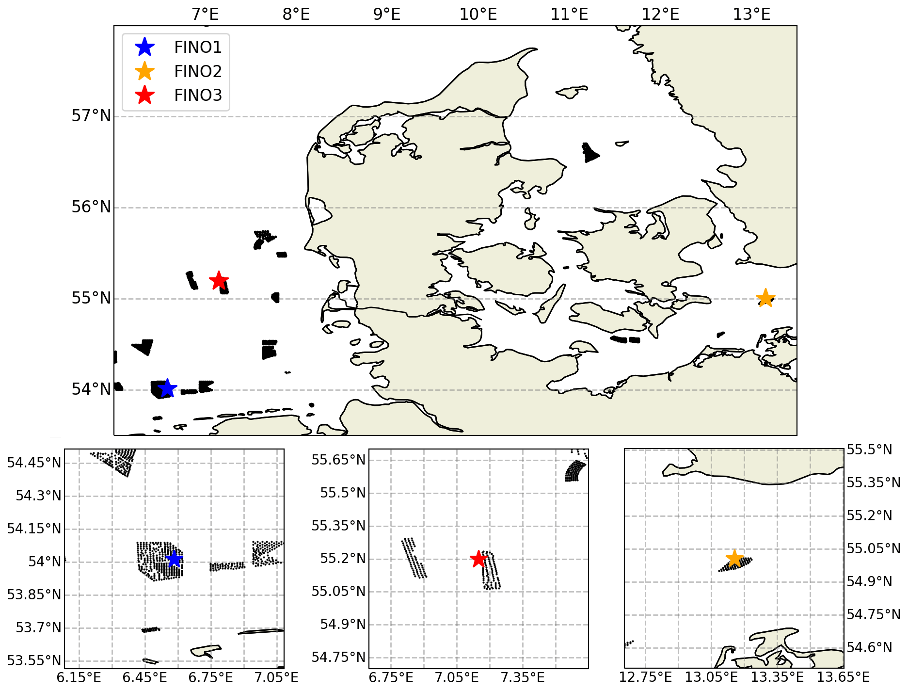
Figure 1 Map of the study area with the FINO mast locations in the North Sea and Baltic Sea (top). The black shapes represent nearby offshore wind farms. The bottom panels show close-ups for the met mast locations with black dots representing individual wind turbines.

Table 1 Characteristics of FINO masts with the heights of available measurements for various meteorological and oceanographic parameters averaged in 30 min intervals.

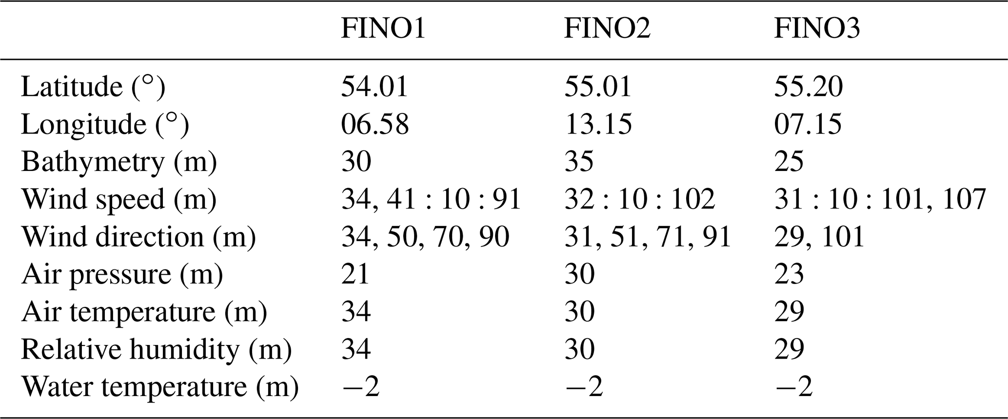
FINO1 is situated in the North Sea approximately 45 km to the north of Borkum, Germany, and in the immediate vicinity of the wind farms alpha ventus and Borkum Riffgrund. The average wind speed is 9.9 m s⁻¹ from 2010 to 2021 at 91 m with a south-westerly prevailing wind. All measurements are available over 90 % of the period of interest, except the water temperature (WT) with 84 % availability.

FINO2 is located in the Baltic Sea, within 3 km north of the EnBW Baltic 2 wind farm and 33 km north of the island of Rügen. The average wind speed is 9.6 m s⁻¹ at 102 m with a south-westerly prevailing wind. All relevant measured variables are available for 90 % of the 12-year period of interest with the exception of WT with 64 % data availability.

FINO3 is located in the North Sea to the west of the DanTysk wind farm, 70 km from the island of Sylt. The average wind speed is 9.6 m s⁻¹ at 107 m over the entire measurement period with a westerly prevailing wind. All measured quantities show a data availability above 85 % with the exception of WT (76 %).

2.3 Satellite sea surface temperature

Besides the water temperature measurements at the met mast locations, which are typically taken at some depth below the surface and are representative of that specific location, space-borne infrared radiometers provide extensive spatial and temporal coverage of the actual sea surface temperature, i.e. SST_skin, which is typically converted to SST_sub-skin and is considered representative of the few top millimetres of the water surface (Donlon et al., 2007). The Copernicus Marine Environment Monitoring Service (CMEMS) releases a suite of level 4, gap-free products with regional and global coverage, representative of the SST foundation temperature, i.e. the temperature free of diurnal warming or nocturnal cooling, typically at the base of the sub-skin layer (Donlon et al., 2007). For the purposes of the present study, the foundation temperature available once per day from the Baltic Sea/North Sea – DMI level 4 (L4) SST – reprocessed L4 analysis was used; it is a gap-free satellite foundation SST analysis created by the Danish Meteorological Institute (DMI) optimal interpolation (OI) system (Høyer and She, 2007). The product is available from 1 January 1982 to 31 May 2021 – it is being temporally extended at regular intervals – on a regular grid with 0.02^∘ resolution. It provides an estimate of the foundation SST with uncertainty estimates, which is the SST free of diurnal variability (Høyer and Karagali, 2016). See CMEMS (2022) for further details.

Data are produced by the Danish Meteorological Institute (DMI) and are distributed by the Copernicus Marine Service (product ID SST_BAL_SST_L4_REP_OBSERVATIONS_010_016, https://resources.marine.copernicus.eu/, last access: 27 April 2023). To diversify from the water temperature measurements available at each meteorological mast site, this product will be referred to as DMI L4 SST for the remainder of this paper. For spatial matching with ASCAT and since the spatial resolution of the DMI L4 SST product is 0.02^∘, a 3×3 grid of SST observations centred in the ASCAT WVC were averaged for each WVC and remapped to the ASCAT coordinates.

2.4 Simulated wind datasets

The NORwegian hindcast Archive (NORA3) is a reanalysis hindcast dataset with a 3 km spatial resolution, available from 1984 to 2021 for the Norwegian Sea, the North Sea and the Barents Sea. NORA3 is dynamically downscaled from the European Centre for Medium-Range Weather Forecasts (ECMWF) ERA5 reanalysis (Hersbach et al., 2020), using the numerical weather prediction (NWP) model HIRLAM–ALADIN (High Resolution Limited Area Model–Aire Limitée Adaptation dynamique Développement InterNational) Research towards Mesoscale Operational NWP In Euromed–Applications of Research to Operations at Mesoscale (HARMONIE–AROME). Three nested domains were used (18, 6 and 2 km horizontal resolution), with a model-integration time of 4 years (2004–2007) and a temporal resolution of 1 h.

The New European Wind Atlas (NEWA) dataset, like NORA3, has a 3 km spatial resolution and is derived from ERA5 reanalysis (Hersbach et al., 2020); however it is downscaled using the WRF model with no data assimilation (Hahmann et al., 2020; Dörenkämper et al., 2020).

Table 2 Input features and heights used to train the random forest model at the FINO met masts. All of the data measured from the FINO masts are 30 min averaged.

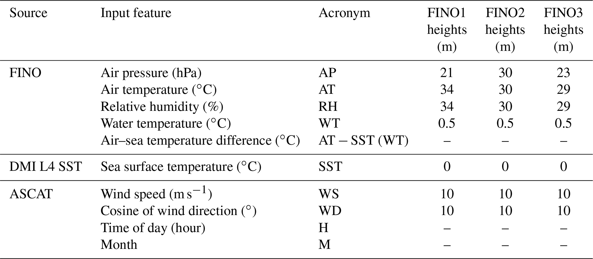
Table 3 Total number of samples used in the random forest model training from each FINO mast at 30 min averages. Note that the “Data used in model training” are 80 % of that of the concurrent data, whereas the “Data used for validation” are 20 %.

For the purpose of this work, only the year 2018 was considered for comparisons due to the concurrent availability of ASCAT and the New European Wind Atlas (NEWA) dataset (Dörenkämper et al., 2020). Due to the different spatial resolution of NORA3 and ASCAT, NORA3 was resampled according to the ASCAT grid; for a given ASCAT WVC, a 3×3 grid of NORA3 grid points centred around that ASCAT WVC was averaged and remapped to the ASCAT coordinates. It should be noted that all data used from all sources are recorded in coordinated universal time (UTC).

2.5 Random forest model

A simple ensemble-based regression tree method known as a random forest model (Breiman, 2001; Hastie et al., 2009) was used in the present study for wind speed extrapolation. A random forest is a collection of decision trees which are trained on random subsets of a training dataset. From the input data, the algorithm generates a forest of N trees $\mathit{\left\{}{T}_{\mathrm{1}}\right(X),T_{\mathrm{2}}(X),\mathrm{\dots },T_N(X\left)\mathit{\right\}}$ using a k-dimensional vector input $X=\mathit{\{}{x}_{\mathrm{1}},x_{\mathrm{2}},\mathrm{\dots },x_k\mathit{\}}$ and a target dataset $Y=\mathit{\{}{y}_{\mathrm{1}},y_{\mathrm{2}},\mathrm{\dots },y_k\mathit{\}}$. These N independent trees predict a final value which is then averaged across all trees: $\stackrel{\mathrm{‾}}{y}=\frac{\mathrm{1}}{N}\sum _{n=\mathrm{1}}^N{T}_n\left(x\right)$, where x is a sample in the testing set and $\stackrel{\mathrm{‾}}{y}$ is the final value. In the case of this study, $\stackrel{\mathrm{‾}}{y}$ will be the predicted wind speed at higher heights (107 m at FINO3 for example), where Y will be the concurrent wind speed measurements at the mast at the desired height. The RandomForestRegressor module in Python's scikit-learn package (Pedregosa et al., 2011), previously used for wind extrapolation in Bodini and Optis (2020) and Optis et al. (2021), was implemented for this study.

Water and air temperature, relative humidity, and air pressure measurements, averaged every 30 min, from each of the three FINO met masts were used as input data (X in the equation above) for the model training along with instantaneous wind speed, cosine of wind direction, time of day and month from ASCAT (see Table 2). The associated number of concurrent samples are shown in Table 3. The fewer samples for the FINO2 mast are associated with the later starting date of WT measurements (2013), resulting in a shorter training period compared to the other two masts, i.e. 7 years for FINO2, 11 years for FINO3 and 14 years for FINO1. Due to the fact that ASCAT collocates with the FINO masts twice a day on average and that all 30 min input data for the model need to be available for the training process, each mast location only yields a training dataset of under 5000 data points. It should be noted that the choice of 30 min averaging of the FINO measurements was to maximize the available collocations. Using larger temporal averaging of 1 h or more would represent a larger portion of data with similar wind statistics but would limit the dataset further due to missing data in the averaging time window.

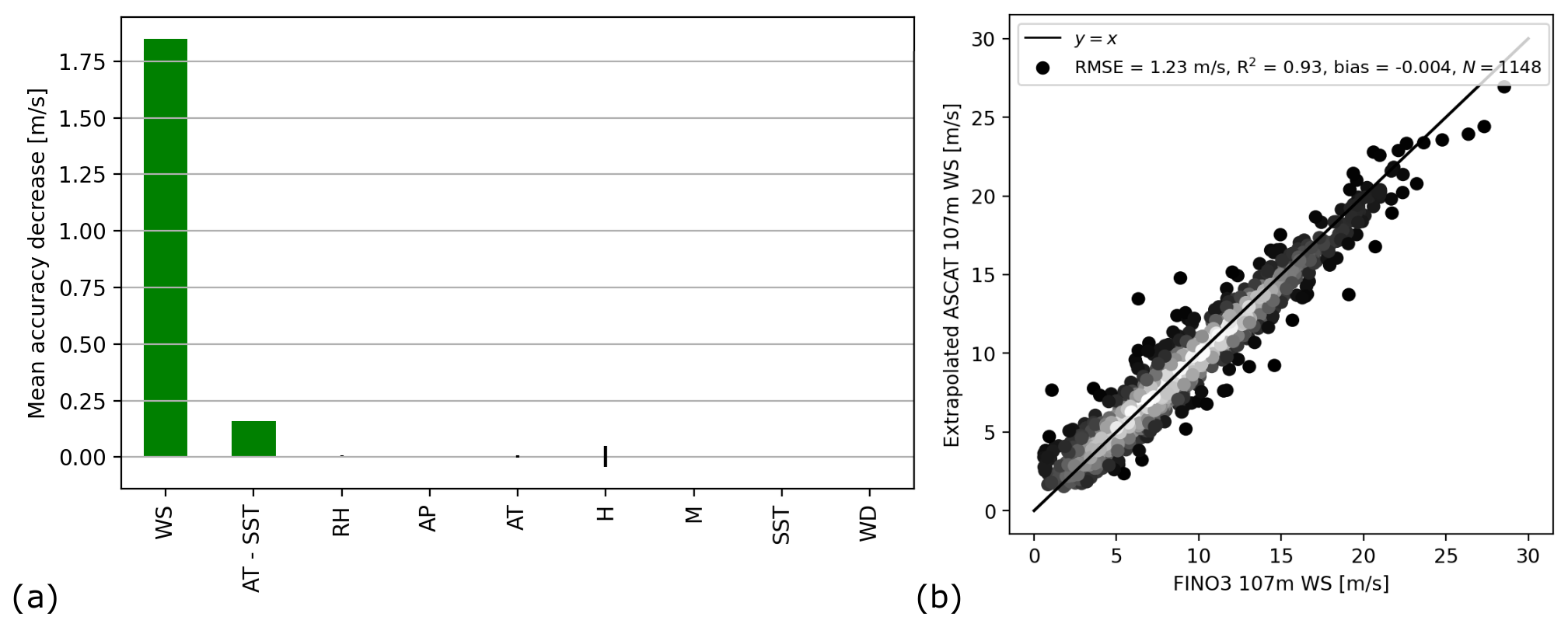
Figure 2 (a) Mean accuracy decrease in the mean square error contribution from the training variables. The small vertical black bars represent the standard deviation of the mean training dataset. (b) Scatterplot of the predicted ASCAT 107 m wind speed (y axis) versus FINO3 107 m wind speed (x axis) measurements, based on the 20 % validation dataset not used in the model-training process.

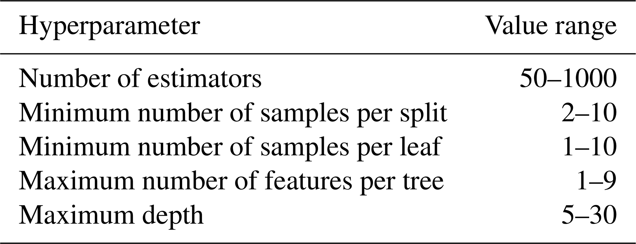
While model parameters are “learned” during the training phase, hyperparameters are set before the training to create a more accurate algorithm. Hyperparameter tuning relies on experimental results of combinations of model parameters to evaluate the performance of each model. The hyperparameters are varied, and their associated ranges are outlined in Table 4. This procedure is repeated for each of the FINO masts.

Table 4 Hyperparameter input range for model cross-validation.

3 Results

3.1 Site selection for random forest model training

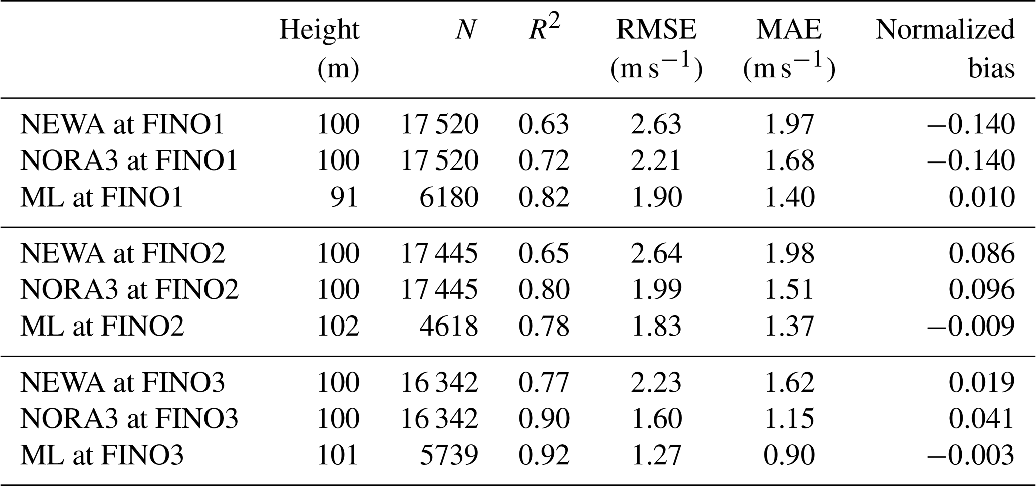
The random forest model was parameterized and trained at each of the three FINO sites, in the North Sea and Baltic Sea. Table 5 shows the metrics of the predicted wind speeds at the highest available heights of each mast: 91 m at FINO1, 102 m at FINO2 and 107 m at FINO3. The models trained at FINO1 and FINO2 have an RMSE of ∼1.8 m s⁻¹ with the test dataset, whereas for FINO3 the RMSE is lower, i.e. ∼1.2 m s⁻¹. The model trained at FINO3 also has the lowest mean absolute error (MAE) as well as the highest coefficient of determination (0.93). At all sites, biases were negligible with the lowest value from the machine-learning output of −0.004 at FINO3. Note that the biases were calculated with respect to the met masts, i.e. $({\stackrel{\mathrm{‾}}{U}}_{\mathrm{pred}}-{\stackrel{\mathrm{‾}}{U}}_{\mathrm{mast}})/{\stackrel{\mathrm{‾}}{U}}_{\mathrm{mast}}$. Both the NEWA and NORA3 datasets have the lowest RMSE, MAE and bias as well as the highest coefficient of determination at the FINO3 site compared to the other sites. The machine-learning model shows lower RMSE and MAE compared to the both the NORA3 and NEWA dataset at all FINO sites for the 2018 comparison. NORA3 consistently outperforms NEWA at all three sites in all metrics except for the bias.

Table 5 Metrics of the NEWA WRF dataset from 2018, NORA3 data from 2018 and the random forest model (ML, machine learning) applied to the entire collocated dataset compared to the wind measurement at the height nearest to 100 m at each of the FINO met masts. Random forest models were trained at each of the FINO met masts using the lowest atmospheric variable measurements available at each height. NEWA and NORA were compared with measurements at each mast at 1 h averages.

Feature importance for the random forest model is calculated based on the increase or decrease in error when permuting over the value of a particular feature. If permuting the values causes a large change in the mean square error (MSE), the feature is an important training criterion for the model. The left panel of Fig. 2 shows the contributions of various input features to the mean model accuracy, with a decrease over the training period for the FINO3 dataset. As expected, the ASCAT 10 m wind speed is the most important feature, while contributions from the other input variables are so small as to be negligible. This behaviour is consistent for the training process at all sites, with the air–sea temperature difference consistently being the second most important training feature. Nonetheless, including the air–sea temperature difference as a feature reduces the overall RMSE by around 20 % at all sites. The right panel of Fig. 2 shows statistics of the predictions at a height of 107 m. Training the dataset at lower heights results in an overall lower RMSE and a higher contribution from the lower atmospheric variables in terms of feature importance; i.e. the air pressure shows a higher contribution to the training for heights up to 80 m (not shown).

In summary, the model-training procedure repeated at the three FINO sites showed the best statistics at FINO3 (Table 5); there, fewer wind farms exist in the vicinity of the meteorological mast compared to the other two sites (Fig. 1) and the highest data availability of wind speed measurements is recorded. For these reasons, focus is given only on this site for the remainder of this study.

3.2 Wind profiles reconstruction

The random forest model (RFM) was used to reproduce the mean wind profile at FINO3, shown in the left panel of Fig. 3, along with that derived from measurements from the mast on site. The model trained in Sect. 3.1 is applied to the entire 12-year collocated dataset at all heights at FINO3 from 31 to 107 m. The observed wind profile (grey dots) shows very low shear, increasing from 8.7 to 9.7 m s⁻¹ between 31 and 107 m. The RFM (black line) performs very well at predicting the mean wind profile. The right panel of Fig. 3 shows the mean wind speed residuals, i.e. the difference between the RFM wind profile and the observed one, at each height. At lower heights, from 31 to 51 m, the model reproduces the wind speeds with a slight over-estimation of just over 0.03 m s⁻¹, while residuals marginally increase at higher heights, indicating a slight over-estimation of the wind profile derived from the RFM. Overall the RFM could reproduce the collocated wind profile at FINO3 with overall very low residuals and slight deviations at higher heights.

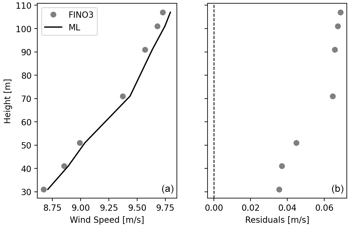
Figure 3 (a) 2010–2021 mean wind profile at FINO3 from the RFM as a line and the corresponding measurements as dots. (b) Wind speed difference between the RFM and the observations.

3.3 Round-robin approach at FINO1 and FINO3

The round-robin approach used here aims at applying the RFM trained at FINO3 to estimate the mean wind speed at FINO1, located 136 km away. Moreover, comparisons with the measurements at FINO1 were performed. For validation purposes, the RFM was optimized through training at the 91 m height of FINO3 using the satellite-based DMI L4 SST product (see Sect. 2.3), instead of the water temperature (WT) measured on site. This optimized RFM was extended to the location of FINO1, where only the ASCAT wind speed/direction and the DMI L4 SST were substituted for the FINO1 site; all other model features, i.e. air temperature, pressure and relative humidity, were assumed to be static, retaining the values used at FINO3.

The RFM-predicted wind speed was evaluated against the wind speeds measured at FINO1 at 91 m (see Table 6). While the change in the bias is negligible, a large increase in RMSE is observed from the original RMSE at the FINO3 site. There is however only a value 8 % higher than the RMSE of the model trained and optimized at FINO1 as seen in Table 6 and an even smaller increase in the MAE.

Table 6 Round-robin model evaluation from FINO3 and FINO1 using the DMI L4 SST product and water temperature (WT) measurements at each site.

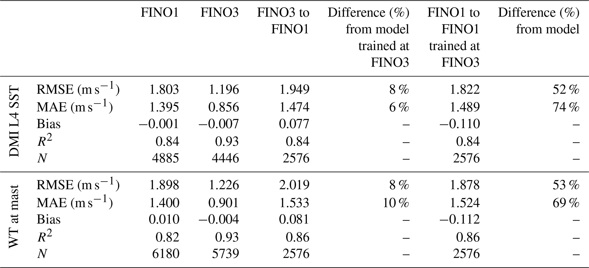
The procedure was repeated by training the RFM using WT measurements at FINO3 (instead of the DMI L4 SST product) and extending it to the FINO1 site using ASCAT wind speed and direction for FINO1, while WT and all other atmospheric parameters remained the same as in the training process, i.e. as measured at FINO3. In this case, the RMSE of the extended model increases by 8 %, with a slightly larger increase in the MAE of 10 %. In using both the DMI L4 SST product and the WT, there was a similar increase in RMSE when extending the model to the FINO1 location, although the increase in MAE is less when using the DMI L4 SST product.

Finally, the procedure was reversed; i.e. a model was trained using FINO1 measurements and extended to FINO3. This was performed twice, i.e. with the DMI L4 SST product and in situ measured WT. A higher RMSE was found in both cases compared to the model trained at FINO3 with both the DMI L4 SST and the mast WT increasing the RMSE by over 50 % alongside a larger associated increase in bias and a very large MAE.

3.4 Spatial extension of the model

To investigate the random forest model performance when the extension is performed over an area around the training site rather than at a single point some distance away, the RFM was trained and extended over an area using two approaches, i.e. the WT measurements from FINO3 and the DMI L4 SST product at each WVC. Results were then compared to the NORA3 reanalysis at each WVC. It should be noted that only NORA3 will be included in the spatial comparison with the RFM as it has out-performed NEWA at the FINO3 mast in Table 5 and in Cheynet et al. (2022) at FINO1.

3.4.1 Including in situ water temperature measurements

Firstly, the RFM was extended over an area defined as 10×10 ASCAT wind vector cells (WVC) centred around FINO3. This was performed using WT and all atmospheric variables measured at FINO3, assuming horizontal homogeneity offshore, while ASCAT wind speed and direction values were used at each WVC.

Figure 4a shows the 2018 mean annual wind field for the study area from the ASCAT 10 m winds, the RFM at 101 m (Fig. 4b) and NORA3 100 m wind speeds (Fig. 4c). This year was selected due to the high availability of ASCAT (MetOp-A, MetOp-B, MetOp-C) and NEWA data availability, as well as the low RMSE between the RFM and measurements at FINO3 (see Table 5).

Figure 4 (a) Mean ASCAT wind speed at 10 m for 2018 around FINO3. (b) RFM-predicted mean wind speed at 101 m for 2018. (c) Mean NORA3 wind speeds at 100 m collocated and regridded to the ASCAT WVCs. (d) Wind speed difference between (b) and (c).

A general increase in wind speed across the entire area can be observed from 10 to 100 m, while the structure and features of spatial variability in the wind field are not maintained. The range of RFM-predicted wind speeds across the study area varies by 0.5 m s⁻¹, from 8.8 to 9.4 m s⁻¹, while in the 10 m ASCAT wind field the speed ranges from 7.5 to 8.2 m s⁻¹, i.e. 0.7 m s⁻¹. In the north-eastern part of the selected area, where the Horns Rev 2 and 3 wind farms are located, a smaller increase in wind speed from 10 to 100 m is observed compared to the surrounding areas. NORA3 shows higher variability of around 1 m s⁻¹, from 9.5 to 10.5 m s⁻¹ with lower wind speeds in the south-eastern area and higher winds in the north-west.

The wind speed difference between the RFM and NORA3 100 m mean winds is shown in Fig. 4d. Wind speed differences of −0.7 m s⁻¹ or larger indicate that the RFM under-predicts the mean wind field compared to NORA3, especially north of the FINO3 location. The smallest wind speed difference occurs in the south-eastern part of the study area, coincidentally near the HelWin wind farm. This agreement can be attributed to the lower wind speeds from NORA3 in this area and the relatively constant wind speed predicted over the entire region.

3.4.2 Including the DMI L4 SST product

Secondly, to assess the impact of SST in the spatial extension of the RFM, unique values from the DMI L4 SST product were used for each WVC along with the unique ASCAT wind speed and direction values, while all other variables remained the same throughout the area of study, i.e. the measurements from FINO3. Figure 5a shows the mean SST for 2018, and the mean RFM 100 m wind field using varying SST is shown in Fig. 5b, while the difference between RFM and NORA3 is shown in Fig. 5d. The RFM wind speeds are higher than what was found when water temperature measurements from the FINO3 site were used throughout the study area (see Fig. 4b); however spatial variability ranges around ∼0.2 m s⁻¹ across the entire region.

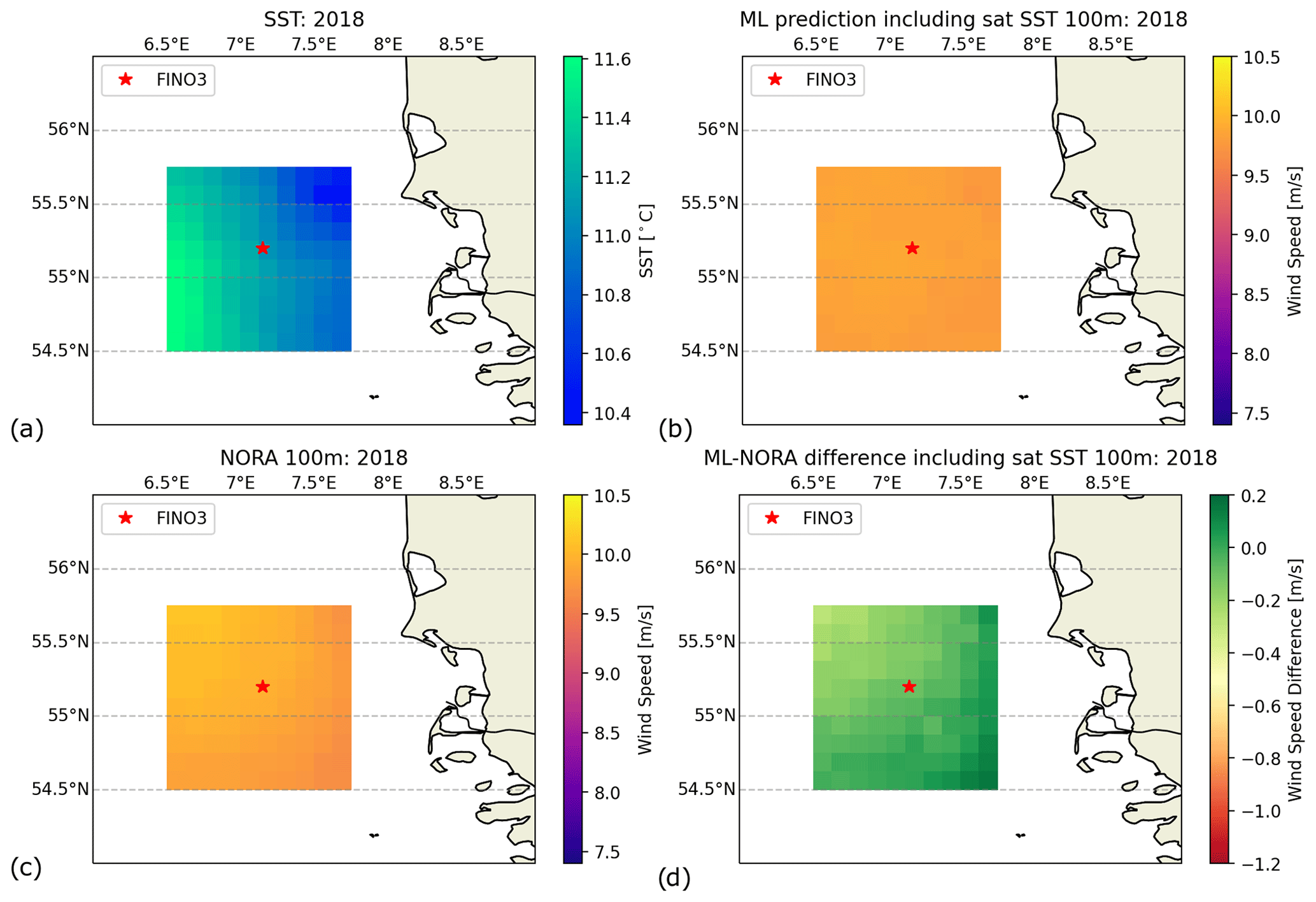
Figure 5 (a) Mean SST for 2018 regridded to the ASCAT WVCs. (b) RFM-predicted wind field at 101 m with varying SST. (c) Mean NORA3 wind speeds at 100 m collocated and regridded to the ASCAT WVCs. (d) Wind speed difference between (b) and (c).

The difference between the RFM, using the DMI L4 SST product at each WVC, and NORA3 100 m winds (see Fig. 5d) indicates a significant change compared to what was found when the measured WT was used for the RFM (see Fig. 4d). The large negative differences on the north-western part of the domain are near zero when the DMI L4 SST product is used in the RFM, while areas that showed small negative biases in Fig. 4d, e.g. south-east, show small positive differences of 0.1 m s⁻¹, indicating a slight over-prediction of the RFM wind speeds compared to NORA3. Contrary to what was shown in Fig. 4d, the highest predicted wind speeds and consequently lowest differences with NORA3 occur in the north-western part of the study area. The nearby wind farms are included in the plot; however there are no clear indications that they have any influence on the predictions, suggesting their contributions are negligible in the ASCAT wind retrievals.

3.5 Data sampling characteristics

The present study is based on training the RFM using discrete, instantaneous retrievals of wind speed and direction from ASCAT rather than the typical 10 min measured time series used in other studies (Vassallo et al., 2020; Bodini and Optis, 2020; Optis et al., 2021). In this section, the effect of discrete sampling on the RFM training is explored utilizing the 12-year-long ASCAT observation period.

Figure 6 shows the number of collocated samples with the FINO3 met mast with each launch of the MetOp satellites. Since the launch of MetOp-B in 2012, a large increase in the number of samples is seen spanning the majority of the training time period.

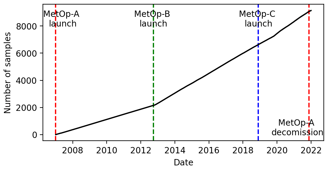
Figure 6 Cumulative number of samples of ASCAT observations at the FINO3 location from 2010–2022. The vertical lines represent the launch of each MetOp satellite as well as the decommission date of MetOp-A.

The number of available ASCAT observations at each WVC of the study area for the years 2010, 2018 and 2020 is shown in Fig. 7. A non-uniform pattern in data availability is observed, associated with the ascending and descending orbits of the MetOp platforms. Note that MetOp-B was launched in 2012 and MetOp-C was launched in November of 2018, while MetOp-A was de-orbited in November 2021. Hence, Fig. 7a only shows observations from one instrument, while in 2018 and 2020 (Fig. 7b and c) two instruments were available, hence the higher range of data availability.

Figure 7 Cumulative samples of ASCAT observations at each WVC of the study area for (a) 2010, (b) 2018 and (c) 2020.

To examine the impact of the sample size, the RFM was trained over different temporal periods and using varying amounts of randomly sampled subsets from the entire collocated dataset. Figure 8a shows the RMSE (top) and bias (middle) between the RFM and FINO3 wind speed measurements at 101 m, along with the number of samples (bottom) when training the RFM each year between 2010 and 2021 at the FINO3 site (black lines). Years were then ranked from lowest to highest RMSE for the 101 m predicted wind speeds which were found in 2012 and 2019, respectively. The evaluation metrics (RMSE and bias) were calculated for the RFM trained on the best performing year, the 2 best performing years, the 3 best performing years, etc. The statistics, shown in Fig. 8a, begin to plateau towards a stable value of RMSE and a negligible bias after 4 years of training when the sample size is around 2500.

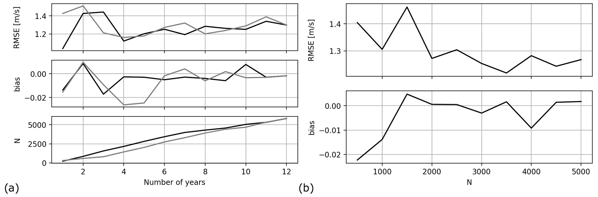
Figure 8 Metric evolution by an incremental number of samples used to train the RFM. (a) Lowest RMSE for individual years trained sequentially (black lines) and sequential training by year from 2010–2021 (grey lines). (b) Training-averaged cumulative random samples of the total dataset.

The same procedure was then repeated for the RFM trained sequentially, i.e. only for 2010, 2010–2011, 2010–2012 and up to the whole period 2010–2021. The RMSE, bias and sample size shown in Fig. 8a (grey lines) indicate that although the bias converges around 4 years (or 2000 samples), the RMSE takes longer time to converge at around 6 years. Convergence of the RMSE and bias towards stable values occurs after 4 (black lines) or 6 (grey lines) years and for just over 2500 samples. In both instances in Fig. 8a the RMSE converges around the 4-year mark between 2000–2500 samples.

Finally, the RFM was trained using random subsamples of the full 12-year dataset instead of yearly subsets. The RMSE and bias between the RFM trained using random subsamples increasing in size and FINO3 wind speed observations at 101 m are shown in Fig. 8b. All metrics appear to be converging to a single value after a given number of samples between 2500 and 3000 – although some metrics plateau around 2000 samples. Results presented here represent 10 averaged instances of training the RFM with increasing random samples.

To investigate the impact of the sample size on the extrapolated wind speed and resulting wind profile, subsets of the 2018 dataset were used to estimate wind profiles shown in Fig. 9a. Just as in Sect. 3.4, the RFM (dashed red line) over-predicts wind speeds at higher heights compared to the FINO3 measurements collocated with the ASCAT observations (red dots). In both cases, the average wind speeds are higher than those estimated from the entire FINO3 measurement period (2010–2021, black crosses).

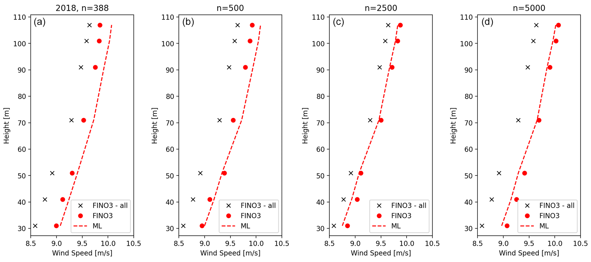
Figure 9 (a) RFM mean wind profile for 2018 using the full dataset. (b–d) RFM wind profile trained on a subset of 500, 2500 and 5000 random samples from the total dataset. Red dots represent FINO3 average wind measurements of the training dataset; black x symbols represent the mean FINO3 values for 2010–2021.

Figure 9b shows mean wind profiles from the RFM trained on 500 samples, around the same size as that of ASCAT in 2018 shown in Fig. 9a; 2500 samples (Fig. 9c); and 5000 samples (Fig. 9d). The RFM (dashed red line) predicts higher winds speeds at heights above 70 m compared to FINO3 measurements for the case of 500 samples (red dots), while both are higher than the complete FINO3 dataset (black crosses). Nonetheless, when increasing the sample size to 2500 (Fig. 9c) and 5000 (Fig. 9d), agreement with the corresponding FINO3 measurements significantly improved. Finally, increasing the sample size from the converging value of n=2500 to higher values, e.g. 5000, showed little to no change in the overall wind speed predictions.

Due to the sun-synchronous nature of the MetOp satellites, the FINO3 location is observed twice per day, in the morning and evening. The number of ASCAT observations as a function of the time of day is shown in Fig. 10, where dark-grey bars represent the entire period and grey bars only represent the year 2018. The majority of ASCAT observations occur between 08:00–10:00 and 19:00–21:00 UTC, with slight variations from 2018. Hourly averaged wind speed measurements from FINO3 at 107 m for the entire period 2010–2021 are shown as a dark-grey line, while the light-grey line represents only the 2018 hourly means. At the ASCAT overpass times, i.e. 08:00–10:00 and 19:00–21:00 UTC, the collocated FINO3 mean wind speed tends to be higher than during the rest of the day, which is more pronounced for 2018 yet also valid for the entire 2010–2021 period. This may provide an explanation for the RFM wind speed over-predictions compared to FINO3 and NORA3. As the RFM is trained using these higher collocated wind speeds, the over-predictions may be related to the temporal sampling of ASCAT.

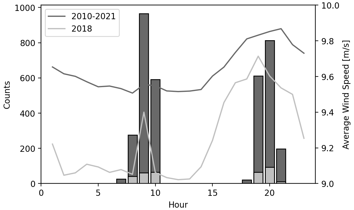
Figure 10 Number of hourly ASCAT observations (bars) at the FINO3 site for 2010–2021 (dark grey) and 2018 (light grey) in UTC. Mean hourly FINO3 wind speed at 107 m (lines) for 2010–2021 (dark grey) and 2018 (light grey).

4 Discussion

This study used machine-learning methods for the extrapolation of ASCAT sea surface wind observations to higher atmospheric levels. A random forest regressor model (RFM) was trained on the near-surface ASCAT wind observations along with measurements of various atmospheric parameters to predict wind speeds at higher heights. The study area included the North Sea and Baltic Sea, specifically the locations of the three FINO meteorological masts. For the assessment of the predicted datasets, simulated winds from NEWA and NORA3 were used. In all occasions the RFM trained at the FINO3 site out-performed the collocated NEWA WRF and NORA3 simulations compared to in situ measurements for 2018, with an RMSE of 1.23 m s⁻¹, an improvement of over 81 % and 30 %. This result is however limited in that the RFM predictions represent a much smaller fraction of the entire FINO datasets compared to the model outputs due to the data availability of ASCAT defined from the polar orbital paths. Results presented in this study indicate the RFM was able to predict mean winds with a similar level of error as that of studies extrapolating low-level winds to hub heights from met mast (Bodini and Optis, 2020), from floating lidar systems (Optis et al., 2021) and with the addition of satellite data (de Montera et al., 2022).

NORA3 was selected for this study as it has been shown to represent the upper percentiles of wind speed much better than ERA5 and the older hindcast NORA10 (Haakenstad et al., 2021). Solbrekke et al. (2021) validated NORA3 against ERA5 reanalysis data, where both wind speed and direction observations from six offshore sites along the Norwegian continental shelf show clear improvement over ERA5 data over both ocean and complex terrain when compared to observational wind speeds. Cheynet et al. (2022) also showed that NORA3 out-preformed the NEWA WRF dataset (Witha et al., 2019) in RMSE, bias and R² at the FINO1 met mast in 2009. NORA3 consistently outperformed NEWA at all three masts for the 2018 study period.

The discrepancies at heights above 51 m in the RFM reconstructed wind profile may be related to atmospheric stratification, as suggested in Optis et al. (2021), where differences between predictions under unstable versus stable conditions were shown. From a similar analysis performed (not shown), results were in agreement with those in Optis et al. (2021); i.e. the RFM was able to capture the unstable profiles but over-predicted the wind profile at higher heights under stable conditions. The effects of atmospheric stability are also encapsulated in the inclusion of the air–sea temperature difference as a feature for the RFM training, similar to Optis et al. (2021), which decreases the RMSE by 20 %. This is further emphasized when the satellite-based DMI L4 SST product was used, specifically for the round-robin comparisons and the spatial extension of the model. In both cases, comparisons with measurements from the met masts and NORA3 improved when the DMI L4 SST product was used.

The impact of including the air–sea temperature difference is evident in the training process as it completely overshadows the other atmospheric and temporal training features with the obvious exception of the satellite-derived wind speed. Without including the air–sea temperature difference there is a larger contribution from the SST and air temperature, while including it decreases the overall RMSE by over 20 %. This was one of the main drivers for including the DMI L4 SST product to the spatial extension of the RFM. An improvement in the RFM model taking NORA3 as reference is seen in Fig. 5a, where the spatial variability in the mean SST field is over 1 ^∘C from east to west, suggesting that the use of a static water temperature measurement at FINO3 is not ideal. However, wind speeds from predictions using the water temperature measurement and assuming horizontal homogeneous FINO3 atmospheric measurements were lower on average by 0.6 m s⁻¹ compared to NORA3 (see Fig. 4d), suggesting that the assumption may still be valid offshore at these distances from the coastline.

One parameter not considered in previous studies, e.g. Bodini and Optis (2020) and Optis et al. (2021), was the length of the training period where it ranged from a few months to a few years of in situ mast or lidar datasets, typically consisting of 10 min measurements. This study uses a discrete subset of satellite wind retrievals, and although it covers a longer period, the number of available observations is smaller compared to 10 min datasets even if the latter extend over shorter periods. Therefore it was considered important to evaluate the model trained over different periods of time. From results presented here, training statistics converged when the sample size increased, reaching a plateau after approximately 2500 samples, suggesting this as a minimum number of samples to properly train a RFM when using satellite observations. This is consistent with findings from Barthelmie and Pryor (2003), where 2000 satellite observations were considered sufficient to represent wind resource statistics. Given the required data availability, only scatterometer winds were used to train the model. SAR winds have higher spatial resolution; nevertheless their data availability is reduced due to a lower temporal-sampling frequency (∼3 d). For areas where SAR winds offer a significant sampling coverage, it would be relevant in a future study to examine their applicability for training RFMs and extrapolating surface winds to higher atmospheric levels.

The authors of de Montera et al. (2022) address the sampling problem with the lack of SAR images (500 samples in their study) with simulating satellite passes with WRF outputs. Similar to this, the RFM method could be applied with supplementary scatterometer data from other missions together with ASCAT. This is expected to provide more robust results from the RFM method. Currently operating missions are HY-2B and HY-2C (Haiyang satellites) with the HSCAT (Haiyang scatterometer) instrument on board launched by the Chinese National Satellite Ocean Application Service (NSOAS) (Zhao et al., 2021). The China–France Oceanography Satellite (CFOSAT) with a scatterometer launched by Centre National d'Études Spatiales (CNES) and China National Space Administration (CNSA) is in operation. CFOSAT winds have been compared to buoy data (Zhu et al., 2022). The Indian Mini Satellite with the SCATSAT-1 scatterometer on board launched by the Indian Space Research Organisation (ISRO) is in operation (Misra et al., 2019). Furthermore, archived data from past missions could be considered such as HY-2A from NSOAS, the SCATSAT-1 satellite with the OSCAT scatterometer on board launched by the ISRO (Wang et al., 2019), and the American QuikSCAT satellite with the SeaWinds scatterometer on board launched by the National Aeronautics and Space Administration (NASA). QuikSCAT observations have been used for wind resource mapping (Karagali et al., 2014). Additional samples from other missions would increase the number of samples and at other times would fill in the diurnal cycle thanks to different orbital paths than ASCAT.

The features used in the machine-learning training process were selected based on their availability to apply the training approach to floating lidar systems in deep-sea environments, since all atmospheric measurements are readily available on current floating lidar systems or through satellite data. Offshore floating lidar systems only provide vertical wind measurements at specific locations, similar to meteorological masts; therefore spatially extending such measurements using two-dimensional satellite wind fields and machine-learning methods is of great interest.

Nonetheless, the need for a large enough sample size of at least 2500 discrete observations may be a limiting factor, as floating lidar systems are typically deployed for periods of 1 to 2 years or less and would not yield the proposed number of collocated observations with the current ASCAT instruments as can be seen in Fig. 6. Using additional satellites such as HSCAT in conjunction with ASCAT could help to address this sampling issue both in terms of the number of collocations and by providing collocation times different than ASCAT. This could aid in addressing the issue of satellites' incapability of capturing the full diurnal wind variability.

Ferry-mounted lidar systems (Gottschall et al., 2018) have been compared with ASCAT winds (Hatfield et al., 2022b); they can also provide spatial sampling not achieved when measurement systems are moored at specific locations. Although the dataset used in Gottschall et al. (2018) covered a period of only 5 months, the concept involves mounting lidar systems on established ferry routes, thus providing the opportunity for longer time series measurements over established paths. Having lidar systems alongside the corresponding atmospheric sensors on already established ferry routes could provide long-term measurements in deep-water areas suitable for training a machine-learning model. Even if there are discrete sampling issues with using satellite data for wind speed extrapolation, a correction bias could be implemented to correct for this, which is however beyond the scope of this work.

With the application of satellite wind retrievals in machine-learning predictions of long-term mean wind speed estimates, the discrete nature of the observations needs to be considered. For the time interval 18:00–21:00 UTC, when ASCAT has the highest sample availability, shown by the bars in Fig. 10, mean winds measured at FINO3 are higher compared to the rest of the day, more pronounced for 2018, as seen in Fig. 10 (lines). This suggests that the temporal dependence of sampling availability may influence the RFM comparisons with NORA3 and in situ measurements at FINO3, especially when limited comparison periods are considered (2018), as artefacts can be introduced because the trained dataset includes features and variability that are not necessarily present during the specific period of comparison. This can potentially explain the slight over-estimation of RFM-predicted winds compared to NORA3 and FINO3 measurements at all heights in Figs. 4d and 5d. This is further supported by results shown in Fig. 9, where for profiles using lower sample sizes, as in Fig. 9a, an over-prediction of both the RFM (red dashed line) and the FINO3 measurements (red dots) is found compared to the profile using all available measurements at FINO3 (crosses).

Bodini and Optis (2020) outlined the importance of applying a round-robin approach when validating models trained in one location to another. While using machine-learning models where hub-height-relevant wind measurement are known to potentially not be of interest, extending those to the area surrounding the training site is of interest, as it can provide a better description of the ambient wind field. In this study, this approach was applied between the FINO1 and FINO3 met masts (as outlined in Table 6). In all cases, a model trained at FINO3 out-performed that at FINO1 in all evaluation metrics. The same result is seen in the comparisons with the NEWA data (see Table 5 and Witha et al., 2019), as well as with the NORA3 data, having an RMSE of 0.8 m s⁻¹ at FINO3 and 1.3 m s⁻¹ at FINO1 (Cheynet et al., 2022). This could be attributed to the proximity of FINO1 to land (45 km) or the high density of wind farms. With a westerly dominated wind direction and located directly in the BorWin wind farms, the wind farm wakes could affect the wind speed measurements at 91 m, having no free-stream wind profiles.

Extending the model spatially and evaluating the results with NORA3 in Figs. 4 and 5 shows that including the satellite SST greatly improve the results. However, in both figures, the RFM was not able to fully reproduce the spatial wind structure as shown in the NORA3 data (Figs. 4c and 5c). Both figures show a resemblance to the ASCAT 10 m wind speeds (Fig. 4a) but with a much narrower range of wind speeds (0.5 and 0.2 m s⁻¹, respectively), where the 10 m wind speed distribution should not be entirely representative of that at 100 m, especially in different atmospheric stability regimes. It can also be noticed that in the ASCAT wind retrievals, in the WVCs enveloping the nearby wind farms, a slightly higher wind speed is observed. This can be attributed to higher reflection caused by the wind farms leading to higher wind retrievals. This can directly impact the RFM, as in both Figs. 4d and 5d the highest wind speed difference with NORA3 is found in the bottom-right WVC, an area with a wind farm and a higher wind speed at 10 m from ASCAT.

5 Conclusions and limitations

The aim of this study was to explore the applicability of machine-learning methods for training a model to extrapolate ocean surface wind measurements from satellites to higher atmospheric levels.

Using a random forest model approach it was possible to effectively recreate the vertical wind profile at FINO3 with only slight over-predictions at the higher atmospheric levels, i.e. between 0.03–0.07 m s⁻¹. A similar pattern was observed when the model was extended over an area of 125 m² surrounding the FINO3 mast. The RFM was found to over-predict the wind speed when compared to the NORA3 reanalysis data over the same area; however including satellite-based SST retrievals over the entire area into the training dataset improved the agreement.

Special attention should be given to the training procedure when using observations with a limited daily temporal resolution, e.g. two to four times per day, as training datasets, such as ASCAT. In those cases, over-/under-prediction of the parameter of interest compared to simulations or in situ measurements may result from the sampling of the original training dataset, regardless of the number of samples used in the training process.

Results from this study show the potential of applying machine-learning methods for the purpose of extrapolating surface winds to higher atmospheric levels. An interesting application of such methods is to use datasets from offshore floating lidar systems specifically for their extension from point measurements to other locations within the area of interest. Such applications would require the availability of measurements spanning at least 2–3 years with the concurrent ASCAT daily coverage with the addition of other satellite measurements such as HSCAT. Extending the period of coverage will not only benefit the available collocated measurements and thus the machine-learning statistics but will also provide a more representative time period for wind resource assessment than the typical 1–2-year timescales.

Although the results are promising, further work is needed to mature this concept of satellite extrapolation with machine-learning techniques. This concept is limited by the fixed sampling rate of the satellite observations and the restrictive training area needing multiyear hub-height wind speed observations. This data-driven methodology does not have the same practical uses as the alternatives used throughout this work for comparisons (i.e. reanalysis or mesoscale models) but is a step towards improving long-term satellite wind measurements for wind energy purposes.