the Creative Commons Attribution 4.0 License.
the Creative Commons Attribution 4.0 License.
 | 17 May 2023
Gaussian mixture models for the optimal sparse sampling of offshore wind resource
Robin Marcille
Maxime Thiébaut
Pierre Tandeo
Jean-François Filipot
Wind resource assessment is a crucial step for the development of offshore wind energy. It relies on the installation of measurement devices, whose placement is an open challenge for developers. Indeed, the optimal sensor placement for field reconstruction is an open challenge in the field of sparse sampling. As for the application to offshore wind field reconstruction, no similar study was found, and standard strategies are based on semi-empirical choices. In this paper, a sparse sampling method using a Gaussian mixture model on numerical weather prediction data is developed for offshore wind reconstruction. It is applied to France's main offshore wind energy development areas: Normandy, southern Brittany and the Mediterranean Sea. The study is based on 3 years of Météo-France AROME's data, available through the MeteoNet data set. Using a Gaussian mixture model for data clustering, it leads to optimal sensor locations with regards to wind field reconstruction error. The proposed workflow is described and compared to state-of-the-art methods for sparse sampling. It constitutes a robust yet simple method for the definition of optimal sensor siting for offshore wind field reconstruction. The described method applied to the study area output sensor arrays of respectively seven, four and four sensors for Normandy, southern Brittany and the Mediterranean Sea. Those sensor arrays perform approximately 20 % better than the median Monte Carlo case and more than 30 % better than state-of-the-art methods with regards to wind field reconstruction error.
- Article
(3149 KB) - Full-text XML
- BibTeX
- EndNote


Offshore wind energy is key in the decarbonation of the global energy production and the reaching of net-zero targets as developed in Shukla et al. (2022). With 11×106 km2 of territorial waters under French jurisdiction and 20 000 km of coastline, France has an extensive and windy seafront. It benefits from the second largest offshore wind potential in Europe, after the United Kingdom, with up to 80 GW of foundation-based offshore wind and 140 GW of floating offshore wind that could be exploited according to IEA (2019). Offshore wind can then be a leading sector for the development of renewable energies in France. The French roadmap currently plans 1 GW of tender per year from 2024 onwards for fixed and floating wind farms. This was confirmed and reinforced in early 2022, with 40 GW of installed capacity envisioned by 2050.
During the development phase of a wind project, the wind resource assessment is a key step to determine its financial feasibility. It can be carried out with numerical weather prediction (NWP) hindcast data such as WRF (Weather Research and Forecasting model) data. However, field observations are necessary to estimate the uncertainties of the models and to assess higher-resolution wind dynamics (Murthy and Rahi, 2017).
Lidars, standing for light detection and ranging, are remote sensing devices that measure wind speed using lasers. Floating lidars are certified devices for offshore wind resource assessment, and they are lidar units integrated onto a standalone floating structure. These wind sensors offer the potential for reduced costs compared to meteorological masts (Gottschall et al., 2017); however, they can be expensive to install and require regular maintenance. Their number and siting thus need to be optimized in order to compose an optimal network of sensors in an offshore wind development area. Such networks are expected to capture most of the dominant wind dynamics from a minimum number of sensors.
Numerous efforts have been undertaken in different scientific fields to optimize sparse sensor siting, a combinatorial problem not solvable by standard approaches such as convex optimization. Sparse sampling is about selecting salient points in a highly dimensional system. It then requires a dimension reduction of the data, such as the use of empirical orthogonal functions (EOFs). EOF analysis projects the original data into an orthogonal basis derived by computing the eigenvectors of a spatially weighted anomaly covariance matrix. Therefore, EOFs of a space-time physical process can represent mutually orthogonal space patterns where the data variance is concentrated, with the first pattern being responsible for the largest part of the variance, the second for the largest part of the remaining variance and so on. EOFs are then very useful for the data reduction of any complex data set such as climate data. By projecting the original data onto a limited subset of relevant orthogonal vectors, it reduces the dimensionality of the system and helps explain the variance of the data. In the past few decades, EOF analyses were used to study spatiotemporal patterns of climate variability, such as the North Atlantic Oscillation, the Antarctic Oscillation and the variability in the Atlantic thermohaline circulation (e.g., Davis, 1976; Thompson and Wallace, 2000; Hawkins and Sutton, 2007; Moore et al., 2013).
EOFs are often at the origin of methods employed to determine the optimal sensor locations for signal reconstruction. In the field of geoscience, Yildirim et al. (2009) employed simulation results from different regional ocean models to define an efficient sensor placement. The authors used the EOF technique to determine the spatial modes of different simulated ocean dynamics systems. The extrema of the EOF spatial modes were found to be good locations for sensor placement and accurate field reconstruction. Zhang and Bellingham (2008) added to the method of empirical orthogonal function extrema (EOF extrema) a constraint on the cross products of EOFs to select the sensor locations and applied it to Pacific sea surface temperature reconstruction. Using the same kind of constrained EOF analysis, Castillo and Messina (2019) proposed a data-driven framework based on a proper orthogonal decomposition (POD) to determine the optimal locations for power system oscillation monitoring and state reconstruction. In this study they selected iteratively the locations with the highest POD amplitude and the lowest cross-coupling between the modes. In Yang et al. (2010), the EOF extrema are used for ocean dynamics reconstruction, introducing an exclusion volume to avoid redundancy and to account for gappy data and for uncertainty.
Manohar et al. (2018) proposed a data-driven method based on a QR pivoting greedy algorithm on a reduced basis to determine optimal sensor placements for face recognition, global sea surface temperature and flow reconstruction around a cylinder. The QR pivoting method decomposes a matrix into an orthogonal matrix and an upper triangular matrix using column pivoting. By iteratively selecting the column with the highest two-norm as pivot, this algorithm for QR factorization is suited for the selection of salient points. In Clark et al. (2020), the QR pivot decomposition is modified to include cost constraints and is applied to the same three data sets. The QR greedy algorithm described in these studies has been used often in recent studies, showing good capabilities and being very easily implementable.
Recent studies proposed innovative methods to improve the capabilities of sparse sampling. To improve the performance of the reconstruction, Chepuri and Leus (2014) proposed a method for grid augmentation to allow for continuous sensor placement, off-grid sensor selection and convex optimization problem formulation. In Mohren et al. (2018), the authors took inspiration from insects' neural activation during flights to derive a sparse sampling method in complex flows to create an encoder for flight mode classification including both the spatial and temporal dependencies of the data. In Fukami et al. (2021), the use of Voronoi tessellation, a method to optimally partition the space into n cells given n input points using a distance measure d, helps to create a viable input for super-resolution from sparse sensors using a convolutional neural network (CNN). This reconstruction technique is then tested on sea surface temperature reconstruction globally, showing the possibility of using sparse sampling on very high-dimension problems.
The problematic of optimal sensor placement has also been investigated for wind energy measurement applications. Annoni et al. (2018) uses the QR greedy algorithm described in Manohar et al. (2018) to determine the optimal locations of sensors to improve the overall estimation precision of the flow field within a wind farm. In this study, the number of sensors is directly computed using a user-defined threshold with regards to reconstruction error. A similar strategy is implemented in this article as presented below. The obtained results show good performance compared to randomly selected grid points, with an improvement of 8 % in flow field reconstruction, and demonstrate the interest in applying sparse sampling methods to the wind energy sector. At even finer scales, Ali et al. (2021) uses low-dimensional classifiers applied to the proper orthogonal decomposition of a large eddy simulation wake simulation to obtain sensor locations for the reconstruction of wind turbine wakes. Using the method of sparse sensor placement optimization for classification described in Brunton et al. (2016), it shows the interest of sparse sampling for the control of wind turbines, using a deep learning algorithm to predict the wake fluctuations from sensor measurements. Results show that most sensors are placed in the transition region, and the reconstruction results in a more than 92 % correlation between predicted and real values.
However, to the best of our knowledge, such methods were never applied at the regional scale for wind energy resource assessment. In our opinion this is due to site selection procedures at the political level that do not necessarily rely on wind resource assessment at the regional level, as well as to smaller required spatial scales at the wind farm developer level, where only one or two sensors are deployed at the extremities of the area, assuming spatial representativity. The application of sparse sampling methodologies to offshore wind reconstruction is an addition of this work. Using NWP spatial wind data as input, the study proposes an unsupervised clustering framework for the identification of salient points in the spatial grid, similar to what can be obtain through EOF extrema analysis in Yildirim et al. (2009) or QR pivoting in Manohar et al. (2018). In the application-driven experimental setup of this study, the two state-of-the-art methods fail to capture wind dynamics at the regional level. Unsupervised clustering automatically discriminates points that are too similar, making it a good candidate for sparse sampling in this case, while keeping the whole method simple and easily implementable.
The objective of the present study is twofold, and the associated problematic is formulated as the following – for conducting offshore wind resource assessment of any targeted area.
-
What is the optimal number of offshore wind sensors to be deployed to best characterize the wind resource?
-
What is the optimal location of each wind sensor?
The optimal number of sensors refers to a trade-off between wind field reconstruction accuracy, and overall cost and computational cost. The optimal locations given a certain number of sensors is the configuration giving the lowest reconstruction error. The two aspects are presented in this work, though realistic cost considerations are not covered.
To do so, this paper presents a data-driven method based on NWP data unsupervised clustering to estimate optimal sensor locations for offshore wind field reconstruction using a Gaussian mixture model. It is compared to state-of-the-art methods used in the above literature (EOF extrema, QR pivoting, randomly selected sensors). The method is then implemented in three areas identified for offshore wind energy development in France. An optimal wind sensor network is proposed for each area to help in the development of offshore wind energy in France.
2.1 Study areas
The three areas investigated in this study are located off the coast Normandy, off the coast of southern Brittany and in the Mediterranean Sea, three major development areas for offshore wind in France with numerous planned offshore projects, listed in Table 1, with future tender processes for respectively 1.5 GW of fixed offshore wind and 250 MW and 2×250 MW of floating offshore wind (expected date of commissioning in 2030).
Table 1Characteristics of the foundation-based (Normandy) and floating (southern Brittany, Mediterranean Sea) future wind farms planned for the next decade in the study areas (CEREMA, 2022). NA signifies not available.

With water depths not exceeding 50 m (Fig. 1), the area located off the coast of Normandy area is particularly suitable for the deployment of fixed offshore wind farms. Current projects will be installed off the coast of Fécamp, Courseulles-sur-Mer and Dieppe – Le Tréport (Fig. 1). The total capacity of each wind farm will be 450–500 MW with a starting date of commissioning expected in 2023–2024 (Table 1). In addition, the French Government has recently announced a new project of a wind farm located 32 km off the coast of Normandy (Fig. 1). This future wind farm will generate 1 GW. The starting date of commissioning is expected by 2028.
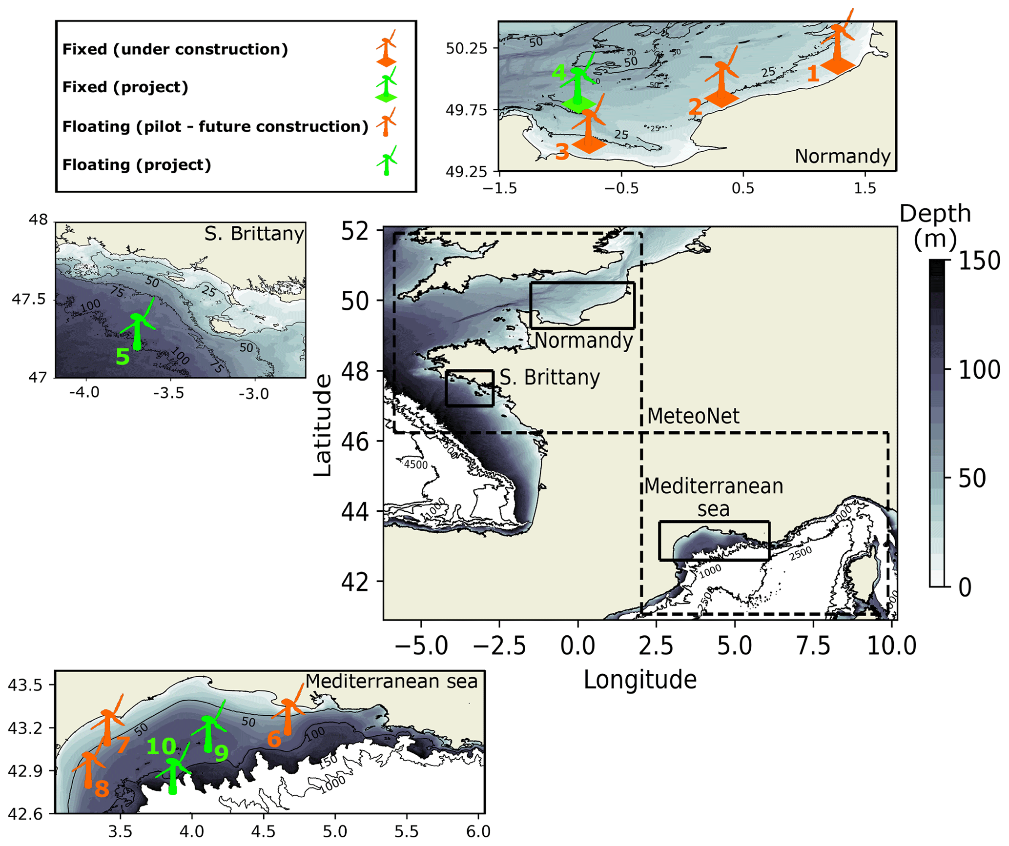
Figure 1Overview of the French coasts with the bathymetry. The color shading shows the water depth until 150 m. Areas with water depths exceeding 150 m are shown in white. Black contours are used to identified depths of 1000, 2500 and 4500 m. The three study areas are shown with black rectangles. Each area is presented on different panels where the locations of the future foundation-based and floating wind farms are shown with their different stages of development. In the main panel, the dashed black lines delimit the areas covered by the MeteoNet data set.
The area off the coast of Brittany has water depths of up to 100 m which makes it a very favorable area for the development of floating wind farms. The French Government aims at developing 250 MW of floating wind energy in the area (Fig. 1).
Because of its very favorable and regular wind regimes and deep bathymetry, the Mediterranean Sea has significant wind potential for floating wind energy. This led to the development of three pilot floating wind farm projects (Leucate, Gruissan and Provence Grand Large) in the Gulf of Lion. These projects will rely on three full-scale 8–10 MW floating turbines, whose generated power will be injected in the French power grid by 2022–2023 (Table 1). In addition, two commercial wind farms with a power capacity of over 250 MW each will be in operation by 2029.
2.2 The MeteoNet data set
MeteoNet is a meteorological data set developed and made available by Météo-France (Larvor et al., 2020), the French national meteorological service. The data set contains full time series of satellite and radar images, NWP models, and ground observations. The data cover two geographic areas of 550 km × 550 km on the Mediterranean and Brittany coasts (Fig. 1) and span from 2016 to 2018. Hourly 10 m wind outputs of the high-resolution NWP model AROME are available. AROME has been operational at Météo-France since December 2008 (Seity et al., 2011). It was designed to improve short-range forecasts of severe events such as intense Mediterranean precipitations, severe storms, fog or urban heat during heat waves. The physical parametrizations of the model come mostly from the Méso-NH research model, whereas the dynamic core comes from the non-hydrostatic model ALADIN (Termonia et al., 2018). The resolution of the AROME grid is 1.3 km. The model is initialized from data assimilation derived from the ARPEGE-IFS variational assimilation system (Courtier et al., 1994) and adapted to AROME's finer resolution.
For each area of interest, the 10 m zonal (u) and meridional (v) wind speeds are extracted from AROME. The open-source MeteoNet data set only contains surface parameters of temperature, humidity, pressure and precipitation, as well as 10 m wind speed (u10, v10), which are considered in this study. The assumption is then made that relevant measurement points at 10 m are equally relevant for hub-height estimation, though this assumption should be tested with a suitable data set. Since the focus is on offshore wind, grid points on land were excluded from the analysis. The characteristics of each area are then the following:
-
Normandy – 4272 grid points (∼ 7000 km2);
-
Southern Brittany – 1837 grid points (∼ 3000 km2);
-
Mediterranean Sea – 3571 grid points (∼ 5800 km2).
A total of 65 d (∼ 6 %) of the 3-year data set are unusable due to largely missing data. The missing data days are similar for each area and were removed from the analysis.
3.1 Problem statement
The problematic of the presented work is to find D measurement points out of K NWP grid points to minimize the reconstruction error in the offshore wind field. A formalism for this sparse sampling problem is proposed in this section.
In all that follows, the full state matrix X refers to the concatenation of zonal and meridional wind speeds on the K grid points of the model for all time steps. The list of sensor locations γ, which is the output of the methods described in this paper, contains the locations of the D sensors to sample the offshore wind field. The associated sparse measurement matrix Yγ corresponds to the measured zonal and meridional wind speeds at the γ locations for every time step.
The formalism developed in this section is applied to the MeteoNet data set presented in Sect. 2.2. The data set is split into a training and a testing period. The training is performed on two-thirds of the data set, composed of the years 2016 and 2017, while the methods are scored on the year 2018. By taking an integer number of year, the seasonality bias of weather data is limited.
3.2 Reduced-order model
The reduced-order model used to decrease the dimension of the input data is the empirical orthogonal function (EOF) analysis. Also known as principal component analysis (PCA), it decomposes the data set into an orthogonal basis. Practically, it is linked to the singular value decomposition of a matrix X such that
with Σ a diagonal matrix of positive σk singular values, U a matrix whose columns are the vectors of the orthogonal basis and V the weights of the associated vectors.
The singular vectors are orthogonal vectors on which the variance of the projected data is maximized. The diagonal elements of Σ are sorted per value and are equal to the percentage of variance of the data set explained by each principal component. The variance explained by the first r EOF is then
The number of EOFs to use in the reduced-order model can be set so that the variance explained by the reduced basis is above a certain threshold.
For the study data set, EOFs of zonal and meridional wind speeds are computed. In the NWP model, the grid points are strongly correlated spatially; hence, only a low number of EOFs is needed to describe the vast majority of the data set variance. The number of EOFs was set to 10 for both the zonal and meridional components of wind so that the reduced basis explains more than 95 % of the total variance for the three areas. The Φr reduced basis is then the concatenation of the and EOFs for zonal and meridional wind speeds, with r=20.
3.3 Sparse sampling
3.3.1 State description
Let us consider a system described by its time-varying state X(t) that evolves according to unknown nonlinear dynamics. It can be described on an orthogonal basis {ϕi} (e.g., the EOF) as
To reduce the complexity of the model, the state of the system can be approximated using the first r modes:
where Φr is the reduced basis matrix containing the first r modes, and ai(t) are the time varying coefficients of the system's state on the reduced basis.
The given system is then sampled according to an index set , γi≠γj, which represents the sensor locations. From this, a sampling matrix is constructed that extracts the D measured locations out of the K grid points of the full state. The sampling matrix is composed of lines of zero with ones at the sensor locations. With the canonical basis vectors , the sampling matrix is
The sparse measurement matrix Yγ is then obtained by multiplying the full state X by the sampling matrix Cγ:
3.3.2 Full state reconstruction from sparse measurements
From the sparse measurement matrix, the full state is reconstructed using the coefficients of the reduced basis. A linear model is constructed to link the matrix of EOF coefficients, a, to the sparse measurement matrix Yγ:
with ϵ an additive Gaussian error.
The model fitting is performed on the training split of the data set. Let Ytrain be the sparse measurement matrix on the training split and atrain the true coefficients of the full state on the reduced basis for the training split. Using the ordinary least squares formula, the β matrix can be estimated as
On the test data set, only the wind speed measurements at the γ locations are available. The coefficients of the reduced basis are computed using the least squares matrix estimated from the training data set:
The full state is reconstructed using the reduced basis:
3.3.3 Reconstruction error
The reconstruction is then compared to the reconstruction with perfect knowledge about the reduced basis coefficients Xreal=Φrareal, assuming that the actual coefficients of the reduced basis are perfectly known.
The reconstruction error associated with the sensor locations γ is then the root mean squared error in the reconstructed state:
The optimization problem that needs to be solved can then be stated as the minimization of the reconstruction error over all locations' combinations γ and number of sensors D:
In this section, the methods applied for the sparse sampling are described in detail. The novel data-driven method based on the Gaussian mixture model is presented, together with the three baselines emerging from the literature review. These are the random selection of locations (Monte Carlo), the dominant spatial mode extrema (EOF extrema) and the QR greedy algorithm (QR pivots). All the methods described in this section should output a list of sensor locations γ given a number of sensors D.
4.1 Baseline methods
The selected baseline methods are emerging from the literature as simple yet efficient methods for sparse sampling in different situations. They are implemented to compare their performances with the Gaussian mixture model for this specific application.
4.1.1 Monte Carlo simulations
The first baseline consists of picking random sensor locations. For each area and for a number D of sensors ranging from 1 to 10, a hundred random combinations of locations are considered. For each γ combination of sensor locations, the reconstruction error is computed. From this ensemble of simulations, statistics on the reconstruction error are computed.
The median Monte Carlo scenario for each area and number of sensors is then considered a benchmark for the study. It also gives information about the spread in reconstruction error resulting from all possible combinations.
4.1.2 Dominant spatial mode extrema
In Yildirim et al. (2009), the extrema of the spatial dominant modes are found to be relevant locations if not optimal for the reconstruction of the flow field. Those points can be seen as salient points that best characterize the spatial modes. It is then intuitive to select those to reconstruct the full state from the reduced basis. How many extrema are chosen from each variable and mode is studied specifically in Cohen et al. (2003); it is empirical and thus case specific.
In the case study of Cohen et al. (2003), the EOF decomposition gives modes that are highly spatially correlated. Moreover, in this study, points near the coast are influenced by the orography and show strong variability. Hence, sorting the points per coefficient and selecting the N first ones will lead to the selection of neighboring points and/or irrelevant coastal points for our performance metric.
The extrema are then chosen manually, as performed in Yildirim et al. (2009), from the visualization of the first EOF for both zonal and meridional wind speeds. For each parameter and EOF rank, the extrema are selected and discarded if redundant (manual process). Then, they are sorted per absolute value and per EOF number for the two parameters.
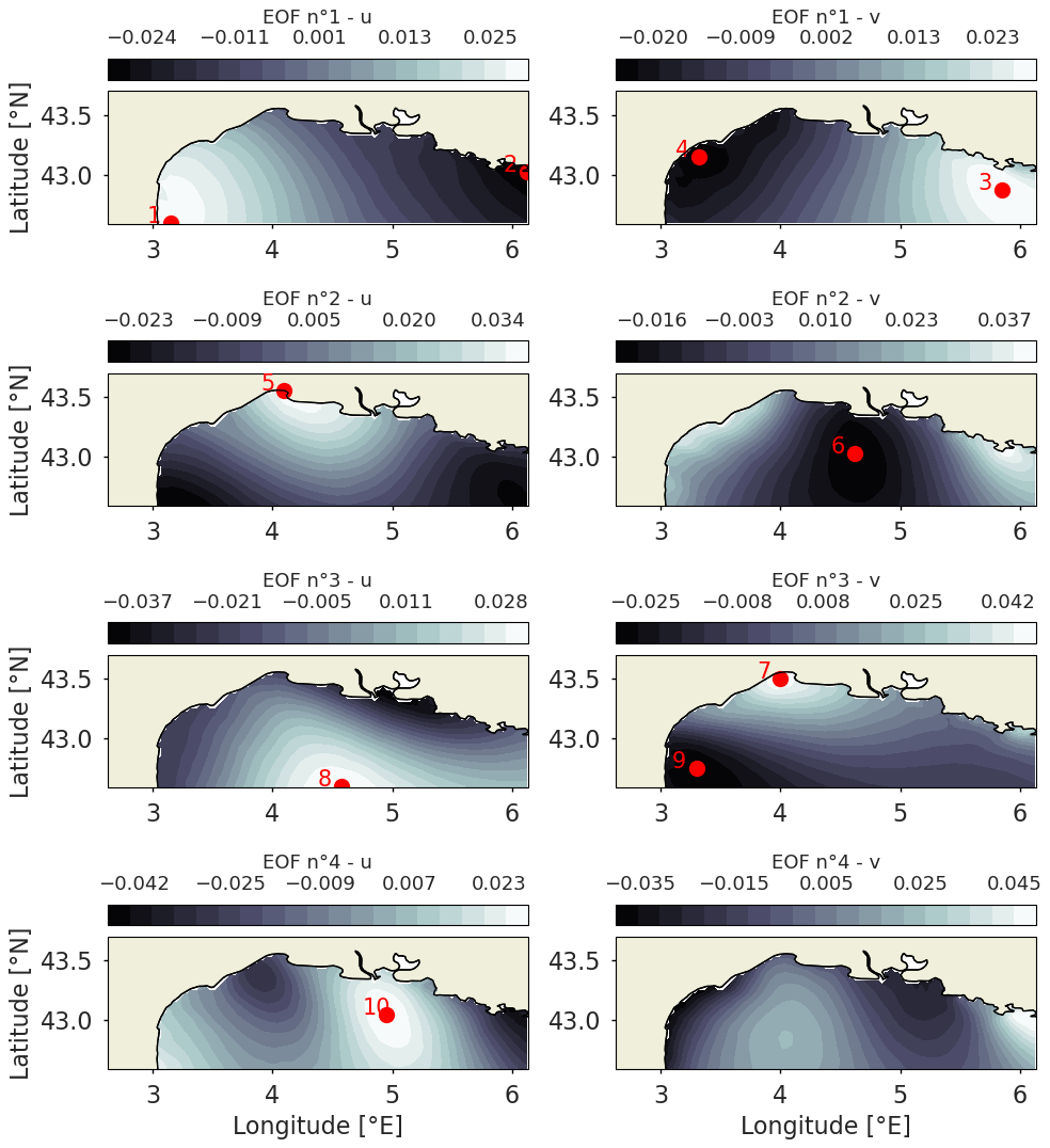
Figure 2Selected sensors for the EOF extrema baseline in the Mediterranean Sea. The EOF coefficients are displayed as background, and the selected salient points and their associated ranks are displayed as red dots. The two columns are zonal (u) and meridional (v) wind speed, and the rows correspond to the EOF rank.
The selected input points from EOF extrema for the Mediterranean Sea are shown in Fig. 2. From the first to the fourth EOFs for zonal and meridional wind speeds, the extrema are selected if they are not too redundant or close to the coast/border. This unsatisfactory workflow is a way to ensure minimum relevance for the obtained sensor array.
4.1.3 QR pivots
The QR decomposition of the reduced basis Φr consists in finding two matrices – orthogonal Q and triangular superior R – such that
The Q and R matrices are obtained using the Gram–Schmidt process (Leon et al., 2013), which consists of iteratively removing each column's orthogonal projection onto a pivot column. The QR algorithm can be performed using column pivoting; i.e., at each iteration, the matrix Φr is multiplied by a permutation matrix P such that the column taken for pivoting has the maximum two-norm. The decomposition is then
The permutation matrix P is constructed so that the diagonal elements of R are decreasing. It is applied to the matrix of the reduced basis to identify pivot locations. It then contains the ranked index of sensor locations to build the sensor location list:
The QR pivot method is described in Manohar et al. (2018) as a simple yet efficient method for sparse sensor placement. It is used to determine model-data-driven sensor networks to reconstruct flow fields for the flow past a cylinder and the sea surface temperature retrieval, two situations that are analogous to the case study. It is even tuned to include cost constraints for the search of Pareto optimal sensor placement in Clark et al. (2020). For wind field estimation, it was applied to computational fluid dynamics data in Annoni et al. (2018) to best reconstruct the flow in a wind farm. All in all, it represents a simple yet competitive baseline method for spare sensor placement.
4.2 Gaussian mixture model clustering
The proposed method in this study uses unsupervised clustering of the data to define sensor locations. Gaussian mixture models use machine learning to fit multivariate normal distributions on the data.
4.2.1 Gaussian mixture
A Gaussian mixture model (GMM) is a probabilistic model for representing normally distributed sub-populations within an overall population (Reynolds, 2009). Each Gaussian distribution represents a group of points, i.e., cluster. The model is a mixture, i.e., superposition, of multivariate Gaussian components which define a probability distribution p(x) on the data:
πj being the mass of the Gaussian component j, with for all , and . being the Gaussian density distribution such that
with x being the r-dimensional input vector, μ the r-dimensional mean vector and Σ (r×r) the covariance matrix.
4.2.2 Expectation–maximization algorithm
The core of the GMM lies within the expectation–maximization (E-M) algorithm, developed by (Dempster et al., 1977). It iteratively modifies the model's parameters to maximize the log likelihood of the data.
The log likelihood, log(ℒ), of the observations is given by
Then the empirical means μj, covariances Σj and weights πj of the different clusters are computed. The weights (mixing coefficients) represent the mass of the different clusters. The mass of the cluster is the proportion of data points assigned to this cluster. For the first iteration, the mean and covariance matrices are initialized randomly, and the weights matrix is equal for each cluster.
The second step of the algorithm is the expectation step, E-step. The model parameters are updated to increase the log likelihood of the data. For each data point, xk, the probability that this point belongs to the cluster, c, is computed such that
The E-step computes those probabilities using the current estimates of the model's parameters. In this step, “responsibilities” of the Gaussian distributions are computed. They are represented by the variables rkc. The responsibility measures how much the cth Gaussian distribution is responsible for generating the kth data point using conditional probability.
The third step is the maximization step, M-step. In this step, the algorithm uses the responsibilities of the Gaussian distributions (computed in the E-step) to update the estimates of the model's parameters. πc, μc and Σc are updated using the following equations:
These updated estimates are used in the next E-step to compute new responsibilities for the data points. This algorithm is applied iteratively until algorithm convergence, when the log likelihood of the data is maximized. The strict monotony of the likelihood in the E-M algorithm is demonstrated in (Wu, 1983).
4.2.3 Optimal number of clusters
GMM requires the number of clusters in the model to be imposed as input. The optimum number of clusters can be defined through the calculation of the Bayesian information criterion (BIC) score (Schwarz, 1978):
with ℒ the maximized value of the likelihood function of the model, G the number of parameters in the mean vectors and covariance matrices of the Gaussian components, and K the number of data points. The BIC score penalizes models that are too complex to avoid the overfitting of the data set. In this way, it limits the number of components of the GMM with the Gln (K) term.
The lower the BIC is, the better the model is. However, the curve of the BIC score can be monotone, and the identification of a minimum, i.e., the optimal number of clusters, can be difficult. An alternative is the calculation of the gradient of the BIC score. The identification of the optimal number of clusters is hence done by the identification of an elbow in the curve of the gradient of the BIC score. The elbow is often not directly associated with one single specific number of clusters but rather encompassed two or three possible solutions. Thus, one can say that the gradient of the BIC score gives an indication of the range of the optimal number of clusters. An extra step is required to determine the optimal number of clusters. In this study, this step is done through the determination of an error reconstruction threshold of the wind field. The number of clusters associated with the minimum error is considered optimal for the GMM.
4.2.4 Implementation for the study case
Figure 3 shows the workflow in this study. A two-dimensional data set composed of K=3571 grid points with 20 EOF features is used to feed the GMM. The 20 features are composed of the first 10 EOFs of zonal and meridional velocities. The clustering is then optimized spatially, so the entries (the grid points) are assigned to clusters based on their features (their coefficients on the first 20 EOFs). The output of the model is then a list of labels for each grid point, creating spatial clusters in the study areas.
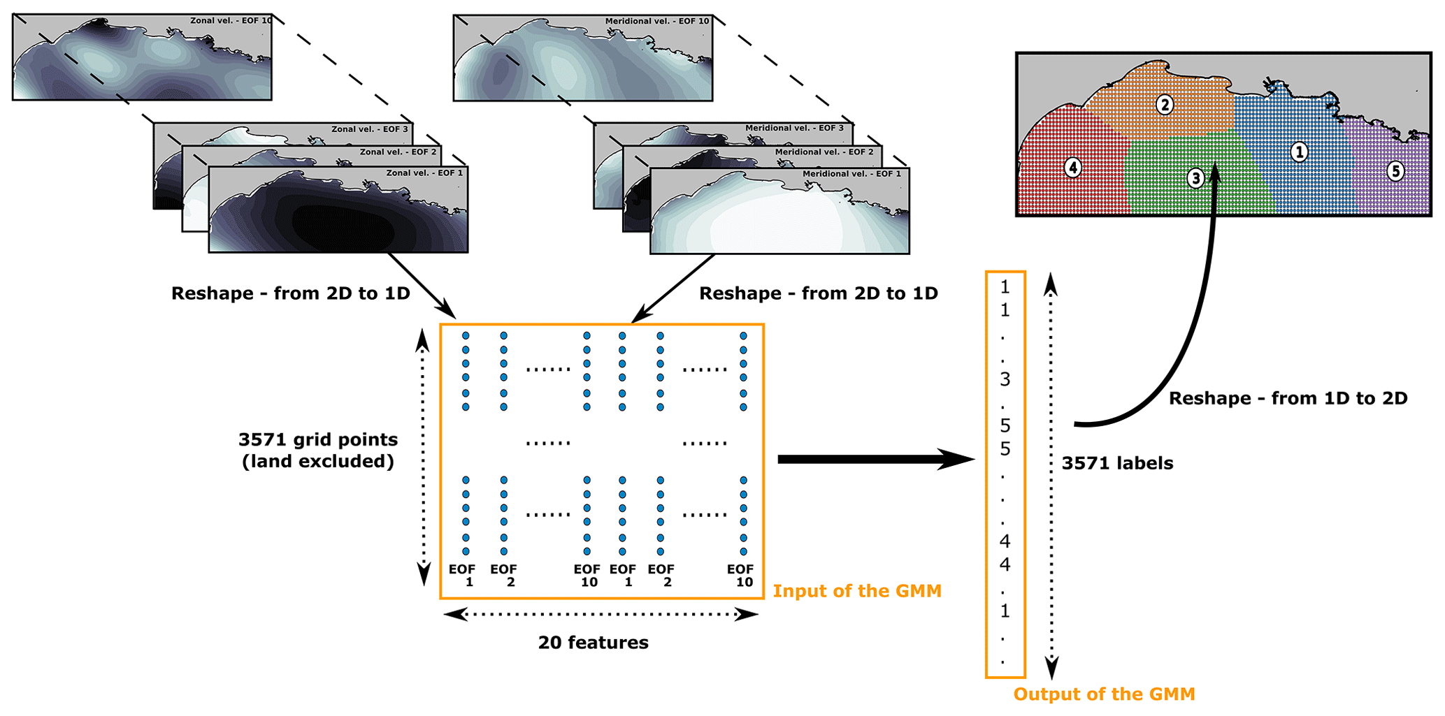
Figure 3Schematic of the clustering procedure of wind data using Gaussian mixture models. It is illustrated for the unsupervised clustering of the Mediterranean Sea wind field.
The GMM procedure will find clusters of grid points that are correlated in the reduced basis. The centroids of the clusters, i.e., the point of maximum likelihood for a given cluster, are then chosen to be sensor locations, as they are the most representative points of the clusters:
In this section, the methods presented in Sect. 4 are implemented in the three identified areas (Mediterranean Sea, Normandy and southern Brittany) and compared with respect to the wind field reconstruction error. A method for the selection of an optimal number of sensors is described, and the suggested sensor locations for the three areas are given.
5.1 Optimal number of sensors
The number of sensors to place on the grid is an input of the GMM. The BIC score described in Sect. 4.2.3 computes a trade-off between the likelihood of the obtained distribution and the complexity of the model. Being sensible to the likelihood of the model and to its complexity, it is usually used to determine the number of clusters for the GMM by finding its minimum. However, there is no guarantee that there will be a minimum BIC score corresponding to an optimal number of clusters, and there is no guarantee that this number of clusters is actually optimal for the considered metric. Indeed, this metric is a heuristic criterion to hint at the trade-off between accuracy and complexity to avoid overfitting. If there is no minimum to the BIC score, one can look for an elbow in the BIC score's gradient, showing a number of clusters after which the marginal gain of BIC score is no longer significant. In this study, the BIC score showed no minimum up to 50 clusters, so its gradient was studied. However, this technique is not very accurate, and the results should be interpreted carefully. For example, the knee identification is very dependent on the cut-in and cut-out of the curve for the definitions of the asymptotes. Furthermore, the GMM results are dependent on the initialization of the algorithm. As shown in Fig. 4, the obtained optimal number of sensors can range between four and seven, though it shows clear convergence for a number of clusters above 10. The gradient of BIC score was computed for 20 random GMM initializations for the three areas, and the mean gradient was plotted as the dashed line, with its 95 % confidence interval as the envelope. The BIC score was normalized to compare the three areas together. Similar trends can be observed, with stronger gradients in the Mediterranean Sea for the first clusters showing a bigger underlying complexity. For southern Brittany, the associated uncertainty is bigger, showing a weaker global minimum for the expectation maximization.
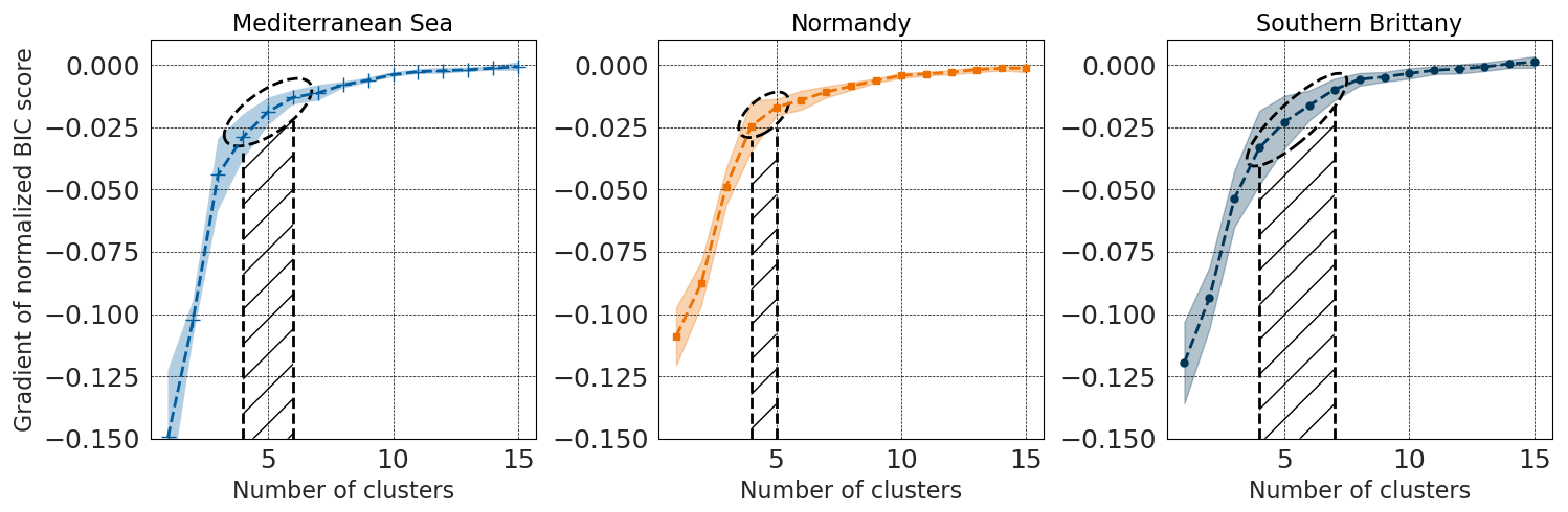
Figure 4The gradient of normalized BIC score is shown for the three areas for a number of clusters ranging from 1 to 15. The curves' envelopes are the 95 % confidence interval obtained from 25 different initializations of the GMM training. The determination of an optimal number of sensors from these curves is uncertain, ranging from four to six for the Mediterranean Sea (shaded area), four to five for Normandy and four to seven for southern Brittany.
While the BIC score gives an indication of the range of optimal number of clusters, it does not necessarily translate into an equivalent reconstruction for the wind fields. Although the clustering itself might find an optimum of five clusters for the Mediterranean Sea, this can lead to a much higher reconstruction error than for the other areas as illustrated in Fig. 5a. In particular for the Mediterranean Sea, the considered region is wider with several different wind regimes, which implies a higher variability. It then seems natural that more sensors than other areas would be needed to reach the same error level. Furthermore, the uncertainty about the optimal number of sensors shows an underlying property of these spatiotemporal data which has strong correlations between points and for which clusters are not well separated. All in all, there is a need to cross-validate the computation of the optimal number of sensors. It is then proposed to validate the number of sensors from the computation of the reconstruction error. Exploring the range of the number of clusters obtained through the BIC score gradient, the final number of sensors is chosen using a reconstruction error threshold.
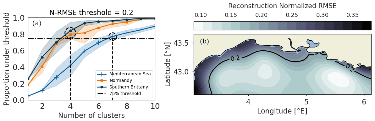
Figure 5The computation of the proportion of the map under a certain error threshold for the three areas and 20 different GMM initializations allows for the selection of the optimal number of sensors as the minimum number of sensors required to reach 75 % of the map under threshold (a). The obtained reconstruction error map with the threshold contour shown illustrates the selection on the Mediterranean Sea (b).
To compare the three areas which have different wind regimes, the error threshold is defined as the reconstruction error in the normalized wind (normalized root mean squared error or N-RMSE). The optimal number of clusters is then computed as the minimal number of clusters required to reconstruct 75 % of the map with an error lower than the threshold.
It is then up to the final user to define an empirical error threshold to derive the optimal scenario. As shown in Fig. 5a, while the BIC score gradient curves are similar for the three areas, the normalized reconstruction error is significantly higher for the Mediterranean Sea for the same number of input points, thus necessitating a higher number of clusters to reach 75 % of the map under threshold. The threshold of 0.2 for the normalized reconstruction error is shown in Fig. 5b. It results in coherent results with regards to the BIC score analysis. The final numbers of clusters are then four each for Normandy and southern Brittany and seven for the Mediterranean Sea. This workflow for the definition of the optimal number of sensors ensures similar performance between the three areas.
5.2 Clustering-derived sensor performance
The sensor locations for the base case scenario with the optimal number of sensors of four each for Normandy and southern Brittany and seven for the Mediterranean Sea are then computed for the three areas for the four methods: Monte Carlo, QR pivoting, EOF extrema and GMM.
The obtained sensor locations are displayed in Fig. 6 as red dots. It can be visually noted that the sensor array derived from the GMM method (second row) is more evenly distributed than the benchmark sensor arrays. QR pivots' locations (third row) are concentrated near the coast or at the maps' limits, and so are EOF extrema (fourth row). It shows how the GMM method allows for homogeneous sampling of the area, while benchmark methods tend to give too much weight to coastal and bordering points. This can be either artificial, due to spatial discontinuity at the limits of the maps, or because of the orographic impact of the coast. Indeed, the wind near the coast shows more variability, and while those points are contained in wider spatial structures in the GMM, they can be considered salient points in the QR pivoting method or in the EOF extrema.
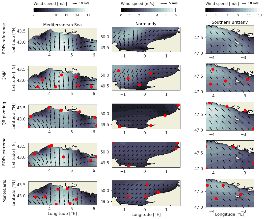
Figure 6Reconstruction example for the optimal scenario in the three areas, from the reduced basis (EOF reference), from GMM clustering (GMM) and from the three baselines: QR pivoting, EOF extrema and Monte Carlo. The color grading shows the wind speed, the black arrows the wind direction with length proportional to the wind speed and the red dots the locations of the sensors in the optimal scenario, with seven sensors in the Mediterranean Sea and four each in Normandy and southern Brittany.
The resulting reconstruction at different time steps is illustrated as background for the three areas and four methods in Fig. 6. The first row is the reference case, reconstructed with perfect knowledge about the 20 EOF coefficients (EOF reference). For the Mediterranean Sea, this specific time step shows a combined Mistral and Tramontane winds blowing in the Mediterranean Sea. It is a complex and standard situation with different wind regimes: strong offshore winds in the north and west of the Gulf and southeastern winds in the eastern extremity. It can be noted that the GMM method correctly reproduces the intensity of those three phenomena, while other techniques tend to overestimate or underestimate their effects.
For Normandy, the benchmark sensor arrays are largely off target in this specific case, predicting little to no wind offshore due to their exclusive coastal sampling, while the GMM method better captures both the coastal low winds and offshore wind cell.
For southern Brittany, the effects of the sensor array is less clear, possibly explained by the smaller area or by a simpler wind regime. However, the GMM method still performs largely better in terms of reconstruction error and wind patterns than benchmark methods.
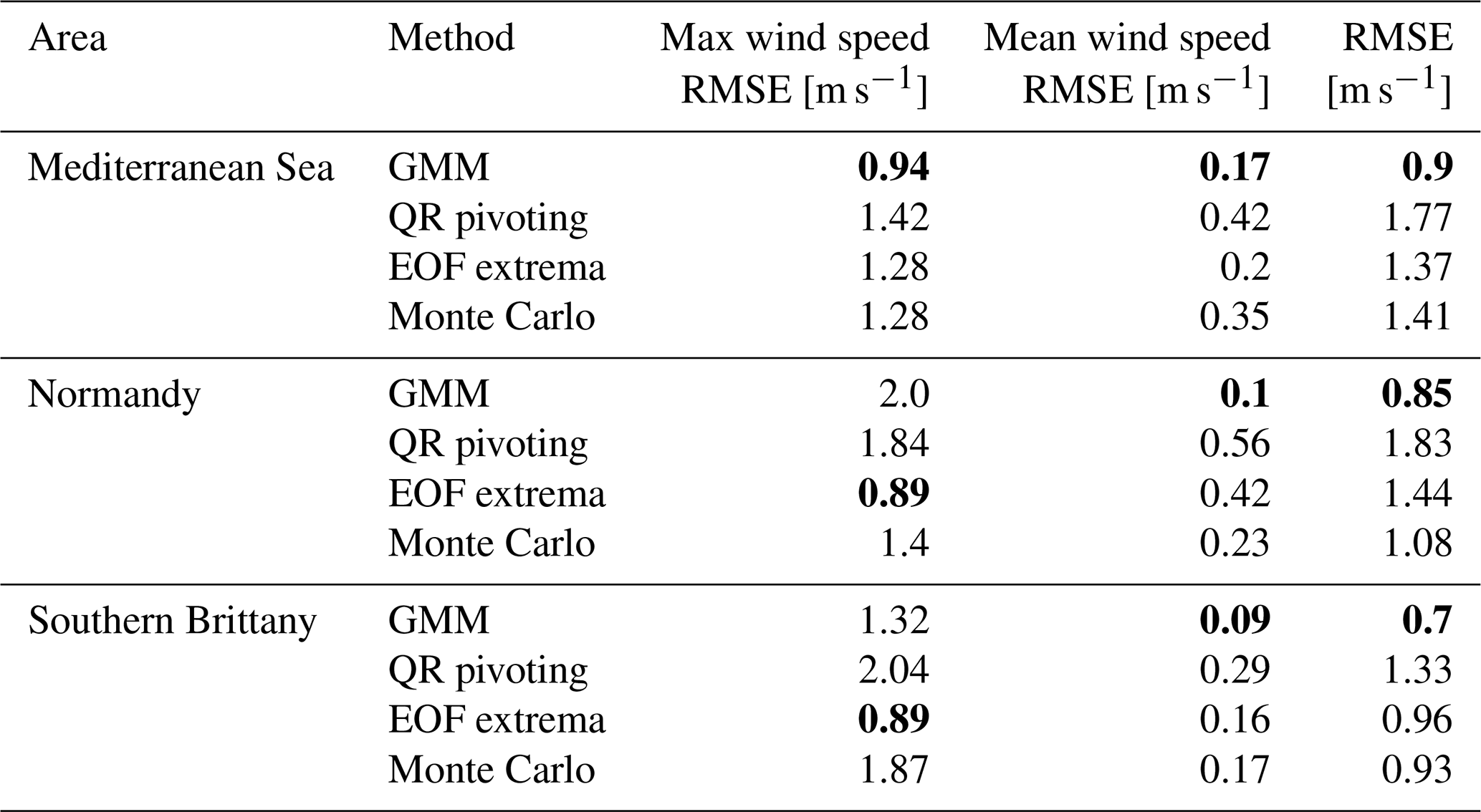
Three different metrics are computed for the optimal scenarios for the three areas and are displayed in Table 2. Along with the reconstruction error described in Sect. 3.3.3, the errors in the reconstructed mean and maximum wind speed are displayed. For the three areas, the GMM method clearly leads to a good reconstruction error and mean wind speed estimation. However, the EOF extrema method results in the better estimation of the maximum wind speed for Normandy and southern Brittany. It illustrates the fact that the GMM method is good at reconstructing the synoptic situation while discarding high variability points that can be relevant for extreme events. Indeed, coastal points that can have a high variability due to the coastal orographic effects are selected as salient points by the EOF extrema and QR pivot and are discarded by the GMM that assigns them to a wider cluster. This is efficient to reconstruct the mean situation in the whole map but can lead to higher errors in high-variability areas.
Table 2Reconstruction errors computed for the three areas and the four sampling methods, including the random scenario displayed in Fig. 6. The best performing method is displayed in bold for each area. The reconstruction error (RMSE) and the errors in the max and mean wind speed at each time step are computed.
The proposed GMM method is scored against the three baselines methods in the Mediterranean Sea area for a number of sensors ranging from 1 to 10. The results are displayed in Fig. 7, showing the great interest of the clustering-derived method compared to benchmark methods for the offshore wind reconstruction from sparse sampling. QR pivoting sensors and EOF extrema sensors fail to surpass the Monte Carlo simulation for a low number of sensors. The GMM method results in reconstruction errors systematically below the minimum of the boxplots (i.e., first quartile minus 1.5 times the interquartile range which is equal to 99.65 % of the data in the Gaussian case), showing the near-optimal reconstruction. The benchmark methods' errors eventually decrease for a high number of sensors and surpass the Monte Carlo median scenario for 10 sensors. However, it is expected that the different methods should converge for a high number of sensors, as the system is more and more constrained. It is illustrated by the decreasing spread within the Monte Carlo simulation.
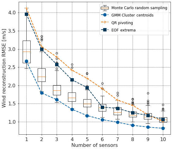
Figure 7QR pivoting method (orange plus), EOF extrema method (deep blue squares) and GMM method (blue dots) are compared to Monte Carlo simulations, displayed as boxplots in terms of wind reconstruction error.
For the GMM curve and the Monte Carlo boxplots, the reconstruction error seems to inflect for a number of sensors around seven, cross-validating the obtained optimal number of sensors for the base scenario. It can be noted that the reconstruction error for the EOF extrema method drastically decreases with the addition of the sixth sensor. As shown in Fig. 2, the sixth sensor is a central offshore point, while the first five locations are near the coast. For a number of sensors above six, the EOF extrema method is then comparable to the Monte Carlo median scenario.
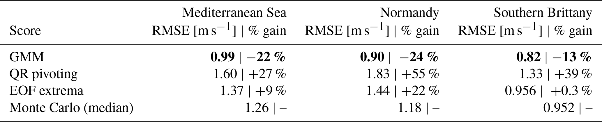
For a low and an optimal number of sensors, compared to state-of-the-art techniques, the GMM method allows for the efficient placement of sensors for offshore wind reconstruction. The obtained reconstruction errors are displayed in Table 3, along with the RMSE gain relative to the Monte Carlo median score. In the three areas, the GMM method improves significantly the reconstruction error in the base case scenario by 13 % for southern Brittany and more than 20 % for Normandy and the Mediterranean Sea. The QR pivoting method proves irrelevant for this application with a 50 % increase in reconstruction error in Normandy and around 30 % in southern Brittany and the Mediterranean Sea. The extrema method is closer to the Monte Carlo median case, though above, probably thanks to the manual removal of irrelevant extrema.
Table 3RMSE and RMSE percentage gain versus Monte Carlo median value for the base case scenario in the three areas for the number of clusters: seven for the Mediterranean Sea and four each for Normandy and southern Brittany. The bold numbers show the best performances.
To visualize the effect of the sensor locations, and the origin of the reconstruction error, the reconstruction error is computed as the root mean square error for each grid point and displayed for the main scenario for the three areas in Fig. 8.
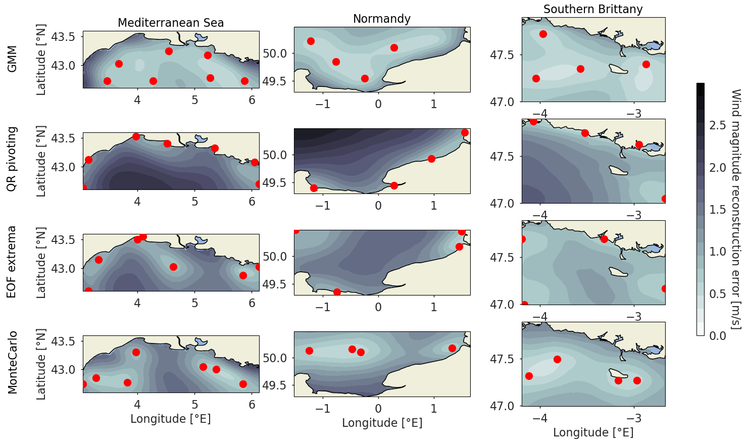
Figure 8Wind magnitude reconstruction error temporally averaged per grid point in the Mediterranean Sea (left), Normandy (center) and southern Brittany (right). The reconstruction error is computed for the optimal number of sensors determined in Sect. 5.1 using the three baselines and the proposed clustering method. The red dots are the grid points used as input for the least squares reconstruction.
The coastal sensor arrays from the QR pivoting method displayed in the second row do not allow for offshore wind reconstruction, as those points are strongly influenced by coastal effects. Strong reconstruction errors of more than 2 m s−1 are then obtained far offshore for Normandy and the Mediterranean Sea. For the EOF extrema method displayed in the third row, where some offshore sensor locations are present in addition to coastal ones, the synoptic wind regime seems better captured with a more homogeneous reconstruction error. The reconstruction error patterns show the strong spatial correlation of the input wind data with lower reconstruction errors around the sensor locations. However, the radius of lowered reconstruction error depends on the location. It can be noted that coastal points in QR pivoting for the Mediterranean Sea have a small radius of influence, as opposed to some offshore points in the EOF extrema method. Coastal areas, where the wind is influenced by the coastal orography and thermodynamic effects, have lower spatial correlations or higher variability. As such, they are considered by the QR pivoting method and the extrema method as salient points. But in the end, they barely help to reconstruct the whole area's dynamics. It illustrates the importance of smart sparse sampling for the reconstruction, as well as the non-adequacy of QR pivots and EOF extrema as locations for the sparse sampling in this case.
For the three areas, the GMM-obtained sensor locations are homogeneously spatially distributed, allowing for good reconstruction on the whole map, though somewhat neglecting coastal locations. The locations, as centroids of clusters, are the most representative points of maximum likelihood clusters for a given number of sensors. As such, every point of the map belonging to a certain cluster, it allows for satisfactory reconstruction on most of the map. On the other hand, the QR pivoting method and EOF extrema method select salient points that do not necessarily correlate well with neighboring points, hence lowering the performance for reconstruction.
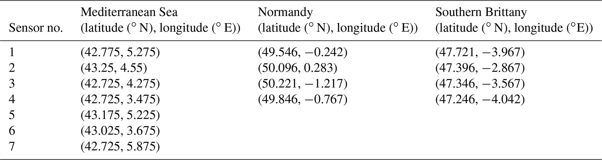
The final suggested sensor locations for the three offshore wind development areas are given in Table 4. These locations should be considered preferred locations for the deployment of floating lidars for wind resource assessment in the French offshore wind development areas.
Table 4Final locations selected for the deployment of floating lidars in French offshore wind development areas.
In this study, an optimal sparse sampling is proposed using a Gaussian mixture model on high-resolution NWP data from Météo-France's MeteoNet data set (AROME model). The method used is simple yet efficient for the optimal sparse sampling of the offshore wind field. Applied to offshore wind resource assessment, it can be a useful tool for the design of observation networks. It is compared to state-of-the-art solutions that fail to efficiently sample this specific problem, and a method is proposed to estimate the optimal number of sensors to deploy. The authors nonetheless draw attention to the following points to interpret and discuss the obtained results.
The metric that is used to measure the performance of the sparse sampling in this paper advantages the GMM method because its homogeneous sampling allows for a correct reconstruction of the synoptic situation. Coastal points are not reconstructed well using the GMM method, but this does not reflect in the scoring. Since the metric averages the reconstructed wind field's error over the grid points, a method that performs fairly well over the entire area is preferred.
As a consequence, both the obtained sensor's location and its performance depend on the selected area. In this study, the selected sites are simple rectangles over the future development areas. But it could be interesting to reconstruct the wind field and score the performance at specific sites defined by operational limits like, for example, bathymetry in the Mediterranean Sea or the coastal exclusion area for the three cases. This could lead to different results, and the sensitivity of the proposed method would then need to be studied.
Given the high variability in the wind near the coast and the possible impact on the obtained results, the first 20 km from the coast were excluded to test the sensitivity of the methods. It roughly corresponds to the distance to the coast for future offshore wind parks and ensures that the impact of the coastal orography is limited. It turns out that it does not make the state-of-the-art methods more relevant for this application as they still tend to select bordering points as input points.
Now, in the context of the development of marine energies in French waters, not only the wind should be considered but other variables such as wave variables and physicochemical parameters (turbidity, sea surface temperature, salinity) which are important for environmental impact monitoring. The installation of a network of sensors would therefore gain traction if optimized with regards to multiple variables. A follow-up of this work would be to include model data for each of the variables of interest and perform the clustering on the stacked first 10 EOFs of each variable for the design of a multiparameter observation network.
Getting even closer to the industrial reality of the sensor networks, it would be of great interest to include a cost function dependent on the location (depth, distance from shore, other constraints). This method could be declined to find the Pareto optimal sensor network. The optimal number of sensors would therefore become the number at which the sensors' marginal cost exceeds the reconstruction gain.
The data in this study are derived from the NWP model AROME data, with a 1.3 km grid size and hourly definition. The parametrization of the model offshore is not perfect, in particular for the sea–atmosphere coupling that can lead to discrepancies in surface parameters, as shown during the Mediterranean HyMex campaign (Rainaud et al., 2016). The dynamics learned might then be a coarse description of the reality, and the derived sensor locations might be limited for real-time wind reconstruction, since they were only trained on low-spatiotemporal-resolution patterns. The obtained locations are in this case optimal only for reconstructing the dynamics of the NWP model, and the representativeness of the data used compared to the reality needs to be questioned. It could then be of interest to run such a study on higher-resolution data, from either synthetic aperture radar measurements or large eddy simulations, though on shorter periods, or comparing the reconstruction to a set of measurements offshore.
Publicly available through the MeteoNet data set, only 10 m wind speed is used in this paper. For offshore wind application, hub-height wind speed is to be considered (heavy maintenance, loading, energy production). The described method is agnostic to the input data, though it would be of interest to validate the obtained sensor network with 100 m wind speed data. It is not directly clear that the obtained sensor network will be the same with data for wind speed above 100 m, since the extrapolation will be depending on the grid point and the wind speed and direction (changing the sea surface roughness). The nonlinear transformation of data can then change the weight given by the clustering model at each time step and grid point.
Seemingly, performing the clustering with the power-curve-transformed data can potentially lead to different results. The study focuses on wind speed, as this can apply to wind energy production but also maintenance operation planning or wind turbine loading. A specific study could focus on wind power, applying vertical extrapolation and wind power curve. The proposed method can be easily implemented in different data inputs.
The data set used compiles 3 years of data. The model is trained on 2 years of data and tested and scored on the third year. It could be of interest to carry out the same study on a longer data set from global reanalysis models such as ERA5. The high-resolution regional AROME model from Météo-France with its 3 years of open-source data from the MeteoNet data set offers a higher number of grid point, making it more relevant for the sensor siting in small areas as the ones in this study. The features that need to be captured by the reconstruction are smaller scale than global models' grid sizes. Comparing the results obtained from the two sources could be of interest.
The benchmark methods used from the sparse-sampling literature, i.e., the QR pivoting method and the EOF extrema method, do not prove to be efficient for the stated problem. For generalization purposes, this method would need to be compared to state-of-the-art methods from benchmark data sets such as the simulated flow past a cylinder used in Manohar et al. (2018). This paper does not aim at generalizing a method but develops an efficient solution to an identified problem, for which state-of-the-art methods seem to fail.
Eventually, the use of a Gaussian mixture model seems appropriate for the sparse sampling of offshore wind resources. It is an easy method to implement with relatively low computational cost. It is flexible and can in principle be applied to higher-dimensional systems. This could be of interest for offshore wind energy, allowing the inclusion of environmental parameters in the siting optimization. The method also shows good consistency in the three development areas tested with very different wind regimes. It is, however, important to stress the difficulty associated with the optimal number of sensors. As proposed in this paper, the number of sensors is derived indirectly from an error threshold. In this context it seems difficult to include cost or environment constraints as such in the sensors siting.
A method for finding an optimal sensor network for offshore wind reconstruction is presented in this paper and applied to three of the main offshore wind energy development areas in France. The sparse sensor placement problem is stated on a reduced basis of the 3-year AROME prediction of wind from the MeteoNet data set. State-of-the-art techniques of sparse sensor placement for reconstruction (QR pivoting and extrema methods) are compared to the proposed method, based on the Gaussian mixture model clustering of empirical orthogonal functions of zonal and meridional wind speeds offshore. By selecting the cluster centroids as proposed locations for sensors, the GMM method homogeneously partitions the domain into spatially correlated clusters. In this way, the reconstruction error in the whole domain is minimized, leading to a 20 % decrease in wind reconstruction error compared to the median Monte Carlo case. On the other hand, state-of-the-art methods fail to reconstruct the whole wind field because they are attracted by salient points with high variability (bordering points). However, these points are not very spatially correlated to neighboring points, resulting in a reconstruction error higher than the median Monte Carlo case. The GMM clustering method gives indications of the optimal number of sensors to deploy, though this estimation should be refined either by the integration of cost or environmental constraints or by the definition of a reconstruction error threshold.
The GMM clustering method seems to be a simple yet efficient solution for sparse sensor placement. Applied to offshore wind reconstruction, it allows for the optimal placement of sensors and paves the way for smart marine monitoring in the era of offshore wind energy development. Further work should focus on the technique's generalization to benchmark problems and question the representativeness of the data set used. For wind energy applications, the multivariate case should be studied for multi-instrumental sensor placement, and the economic constraints should be implemented for the definition of the Pareto optimal number of sensors.
In light of this study, the authors suggest the deployment of seven sensors in the Mediterranean Sea, four sensors in Normandy and four sensors in southern Brittany at optimal locations to reconstruct the offshore wind field and to help with the wind resource assessment on these areas.
Meteorological data used in this study are available online through the MeteoNet data set. The code developed for offshore wind resource sparse sampling using Gaussian mixture models can be accessed through https://github.com/rmarcille/gmm_sparse_sampling.git (last access: May 2023; https://doi.org/10.5281/zenodo.7835596, Marcille and Thiébaut, 2023).
JFF and MT identified the problematic. MT and PT designed the experiment. RM carried out the experiment and performed the simulations under the supervision of MT and PT. MT and RM developed the model code. RM prepared the manuscript with contributions from all co-authors
The contact author has declared that none of the authors has any competing interests.
Publisher’s note: Copernicus Publications remains neutral with regard to jurisdictional claims in published maps and institutional affiliations.
This research has been supported by France Energies Marines and the French Government, managed by the Agence Nationale de la Recherche under the Investissements d’Avenir program, with the reference ANR-10-IEED-0006-34. This work was carried out in the framework of the FOWRCE_SEA and POWSEIDOM projects.
This paper was edited by Sara C. Pryor and reviewed by Sarah Barber and three anonymous referees.
Ali, N., Calaf, M., and Cal, R. B.: Clustering sparse sensor placement identification and deep learning based forecasting for wind turbine wakes, J. Renew. Sustain. Ener., 13, 023307, https://doi.org/10.1063/5.0036281, 2021. a
Annoni, J., Taylor, T., Bay, C., Johnson, K., Pao, L., Fleming, P., and Dykes, K.: Sparse-sensor placement for wind farm control, J. Phys.-Conf. Ser., 1037, 032019, https://doi.org/10.1088/1742-6596/1037/3/032019, 2018. a, b
Brunton, B. W., Brunton, S. L., Proctor, J. L., and Kutz, J. N.: Sparse Sensor Placement Optimization for Classification, SIAM J. Appl. Math., 76, 2099–2122, https://doi.org/10.1137/15M1036713, 2016. a
Castillo, A. and Messina, A. R.: Data-driven sensor placement for state reconstruction via POD analysis, IET Generation, Transmission & Distribution, 14, 656–664, 2019. a
CEREMA: Eoliennes en mer en France, https://www.eoliennesenmer.fr/ (last access: May 2023), 2022. a
Chepuri, S. P. and Leus, G.: Continuous sensor placement, IEEE Signal Proc. Let., 22, 544–548, 2014. a
Clark, E., Kutz, J. N., and Brunton, S. L.: Sensor Selection With Cost Constraints for Dynamically Relevant Bases, IEEE Sens. J., 20, 11674–11687, https://doi.org/10.1109/JSEN.2020.2997298, 2020. a, b
Cohen, K., Siegel, S., and McLaughlin, T.: Sensor Placement Based on Proper Orthogonal Decomposition Modeling of a Cylinder Wake, in: 33rd AIAA Fluid Dynamics Conference and Exhibit, 4259, https://doi.org/10.2514/6.2003-4259, 2003. a, b
Courtier, P., Thépaut, J.-N., and Hollingsworth, A.: A strategy for operational implementation of 4D-Var, using an incremental approach, Q. J. Roy. Meteor. Soc., 120, 1367–1387, 1994. a
Davis, R. E.: Predictability of sea surface temperature and sea level pressure anomalies over the North Pacific Ocean, J. Phys. Oceanogr., 6, 249–266, 1976. a
Dempster, A. P., Laird, N. M., and Rubin, D. B.: Maximum Likelihood from Incomplete Data Via the EM Algorithm, J. R. Stat. Soc. B, 39, 1–22, https://doi.org/10.1111/j.2517-6161.1977.tb01600.x, 1977. a
Fukami, K., Maulik, R., Ramachandra, N., Fukagata, K., and Taira, K.: Global field reconstruction from sparse sensors with Voronoi tessellation-assisted deep learning, Nature Machine Intelligence, 3, 945–951, 2021. a
Gottschall, J., Gribben, B., Stein, D., and Würth, I.: Floating lidar as an advanced offshore wind speed measurement technique: current technology status and gap analysis in regard to full maturity, WIREs Energy Environ., 6, e250, https://doi.org/10.1002/wene.250, 2017. a
Hawkins, E. and Sutton, R.: Variability of the Atlantic thermohaline circulation described by three-dimensional empirical orthogonal functions, Clim. Dynam., 29, 745–762, 2007. a
IEA: Offshore Wind Outlook 2019, Tech. rep., IEA, https://www.iea.org/reports/offshore-wind-outlook-2019 (last access: May 2023), 2019. a
Larvor, G., Berthomier, L., Chabot, V., Le Pape, B., Pradel, B., and Perez, L.: MeteoNet, An Open Reference Weather Dataset by Meteo-France, Météo France [data set], https://meteonet.umr-cnrm.fr/ (last access” May 2023), 2020. a
Leon, S. J., Björck, Ã., and Gander, W.: Gram-Schmidt orthogonalization: 100 years and more, Numer. Linear Algebr., 20, 492–532, https://doi.org/10.1002/nla.1839, 2013. a
Marcille, R. and Thiébaut, M.: rmarcille/gmm_sparse_sampling: gmm_sparse_sampling_v1.0.0 (article_version), Zenodo [code], https://doi.org/10.5281/zenodo.7835596, 2023. a
Manohar, K., Brunton, B. W., Kutz, J. N., and Brunton, S. L.: Data-Driven Sparse Sensor Placement for Reconstruction: Demonstrating the Benefits of Exploiting Known Patterns, IEEE Contr. Syst. Mag., 38, 63–86, https://doi.org/10.1109/MCS.2018.2810460, 2018. a, b, c, d, e
Mohren, T. L., Daniel, T. L., Brunton, S. L., and Brunton, B. W.: Neural-inspired sensors enable sparse, efficient classification of spatiotemporal data, P. Natl. Acad. Sci. USA, 115, 10564–10569, 2018. a
Moore, G. W. K., Renfrew, I. A., and Pickart, R. S.: Multidecadal mobility of the North Atlantic oscillation, J. Climate, 26, 2453–2466, 2013. a
Murthy, K. S. R. and Rahi, O. P.: A comprehensive review of wind resource assessment, Renewable and Sustainable Energy Reviews, 72, 1320–1342, 2017. a
Rainaud, R., Lebeaupin Brossier, C., Ducrocq, V., Giordani, H., Nuret, M., Fourrié, N., Bouin, M.-N., Taupier-Letage, I., and Legain, D.: Characterization of air–sea exchanges over the Western Mediterranean Sea during HyMeX SOP1 using the AROME–WMED model, Q. J. Roy. Meteor. Soc., 142, 173–187, 2016. a
Reynolds, D. A.: Gaussian mixture models, Encyclopedia of biometrics, 741, 659–663, 2009. a
Schwarz, G.: Estimating the dimension of a model, Ann. Stat., 1st edition, https://doi.org/10.1214/aos/1176344136, 461–464, 1978. a
Seity, Y., Brousseau, P., Malardel, S., Hello, G., Bénard, P., Bouttier, F., Lac, C., and Masson, V.: The AROME-France convective-scale operational model, Mon. Weather Rev., 139, 976–991, 2011. a
Shukla, P., Skea, J., Slade, R., Al Khourdajie, A., van Diemen, R., McCollum, D., Pathak, M., Some, S., Vyas, P., Fradera, R., Belkacemi, M., Hasijaand, A. Lisboa, G., Luz, S., Malley, J. (Eds.): Climate Change 2022: Mitigation of Climate Change. Working Group III Contribution to the IPCC Sixth Assessment Report, Tech. rep., IPCC, Cambridge, UK and New York, NY, USA, https://www.unep.org/resources/report/climate-change-2022-mitigation-climate-change-working-group-iii-contribution-sixth (last access: May 2023), 2022. a
Termonia, P., Fischer, C., Bazile, E., Bouyssel, F., Brožková, R., Bénard, P., Bochenek, B., Degrauwe, D., Derková, M., El Khatib, R., Hamdi, R., Mašek, J., Pottier, P., Pristov, N., Seity, Y., Smolíková, P., Španiel, O., Tudor, M., Wang, Y., Wittmann, C., and Joly, A.: The ALADIN System and its canonical model configurations AROME CY41T1 and ALARO CY40T1, Geosci. Model Dev., 11, 257–281, https://doi.org/10.5194/gmd-11-257-2018, 2018. a
Thompson, D. W. and Wallace, J. M.: Annular modes in the extratropical circulation. Part I: Month-to-month variability, J. Climate, 13, 1000–1016, 2000. a
Wu, C. F. J.: On the Convergence Properties of the EM Algorithm, Ann. Stat., 11, 95–103, https://doi.org/10.1214/aos/1176346060, 1983. a
Yang, X., Venturi, D., Chen, C., Chryssostomidis, C., and Karniadakis, G. E.: EOF-based constrained sensor placement and field reconstruction from noisy ocean measurements: Application to Nantucket Sound, J. Geophys. Res.-Oceans, 115, C12072, https://doi.org/10.1029/2010JC006148 , 2010. a
Yildirim, B., Chryssostomidis, C., and Karniadakis, G. E.: Efficient sensor placement for ocean measurements using low-dimensional concepts, Ocean Model., 27, 160–173, 2009. a, b, c, d
Zhang, Y. and Bellingham, J. G.: An efficient method of selecting ocean observing locations for capturing the leading modes and reconstructing the full field, J. Geophys. Res.-Oceans, 113, C04005, https://doi.org/10.1029/2007JC004327, 2008. a