Experimental validation of a short-term damping estimation method for wind turbines in nonstationary operating conditions

Modal properties and especially damping of operational wind turbines can vary over short time periods as a consequence of environmental and operational variability. This study seeks to experimentally test and validate a recently proposed method for short-term damping and natural frequency estimation of structures under the influence of varying environmental and operational conditions from measured vibration responses. The method is based on Gaussian process time-dependent auto-regressive moving average (GP-TARMA) modelling and is tested via two applications: a laboratory three-storey shear frame structure with controllable, time-varying damping and a flutter test of a full-scale 7 MW wind turbine prototype, in which two edgewise modes become unstable. Damping estimates for the shear frame compare well with estimates obtained with stochastic subspace identification (SSI) and standard impact hammer tests. The efficacy of the GP-TARMA approach for short-term damping estimation is illustrated through comparison to short-term SSI estimates. For the full-scale flutter test, GP-TARMA model residuals imply that the model cannot be expected to be entirely accurate. However, the damping estimates are physically meaningful and compare well with a previous study. The study shows that the GP-TARMA approach is an effective method for short-term damping estimation from vibration response measurements, given that there are enough training data and that there is a representative model structure.

1 Introduction

A novel operational modal analysis (OMA) method (Ebbehøj et al., 2023) for short-term modal damping estimation for structures under the influence of varying environmental and operational conditions (EOCs), such as wind turbines in operation, is tested with a controlled laboratory experiment and a wind turbine flutter test.

The dynamic properties of wind turbines (i.e. natural frequencies, damping ratios, and mode shapes) can be sensitive to changing EOCs (Avendaño-Valencia et al., 2017; Bogoevska et al., 2017). Aeroelasticity, active control, material properties, and nonlinear damping mechanisms (e.g. friction) are examples of phenomena and factors which can cause EOC variability (M. O. Hansen et al., 2006; Wang et al., 2022; Chen and Duffour, 2018). EOC variability can act on short and long timescales relative to the fundamental frequency of the given structure. For example, changing temperatures of wind turbine towers affecting their natural frequencies work on the order of hours and days (Hu et al., 2015), which in this context are considered long-term effects. By contrast, complex aero–servo–elastic interactions of multi-megawatt wind turbines can cause short-term variability of damping in particular over a few minutes due to dependencies on e.g. rotor speed, blade pitch angle, and wind speed (M. O. Hansen et al., 2006; M. H. Hansen et al., 2006).

Estimating aeroelastic (or operational) damping accurately is essential for improving the design of multi-megawatt wind turbines, as it is a crucial design parameter for modelling fatigue and aeroelastic instabilities, i.e. stall-induced vibrations (SIVs) and vortex-induced vibrations (VIVs) (Veers et al., 2023). Improved aeroelastic damping estimation may therefore enable designs associated with less risk or less material usage. However, “a precise evaluation of aeroelastic damping remains an elusive goal in some operating conditions”, as stated in Grand challenges in the design, manufacture, and operation of future wind turbine systems (Veers et al., 2023, p. 1090). The combination of nonstationary EOCs and EOC-sensitive damping complicates the task of obtaining precise aeroelastic damping estimates for wind turbines.

OMA covers a broad class of output-only system identification methods for estimating modal parameters for structures in operating conditions where the input (i.e. forcing or excitation) is not measured. Standard OMA techniques, for instance, the covariance-driven stochastic subspace identification (COV-SSI) (Peeters and Roeck, 2001; Brincker and Ventura, 2015), typically assume the system is linear and time invariant (LTI) with input resembling stationary white noise and requiring long time measurements. Brincker and Ventura (2015) suggest a minimum measurement time of $\frac{\mathrm{10}}{f\mathit{\zeta }}$, where fζ is the lowest natural frequency–damping ratio multiple of a given structure. This translates to a measurement time requirement of approximately 28 min for a mode with a natural frequency of 0.2 Hz and 3 % damping ratio, which is in the range of a multi-megawatt wind turbine mode. Therefore, the capabilities to track short-term variations in damping are limited for these methods.

When identifying modal damping from output-only measurements, the effect of input on the measured output must be accounted for since both input and damping govern the near-resonant vibration amplitudes. This can be done by either eliminating the effect (i.e. averaging it out) or modelling it (Au, 2017). Standard OMA methods rely on the former approach. For instance, in COV-SSI covariance, Toeplitz matrices of the output measurements are computed and used as equivalent free response approximates of an assumed LTI system (Peeters and Roeck, 2001). However, a considerable amount of data is required (minimum measurement time of $\frac{\mathrm{10}}{f\mathit{\zeta }}$) for the covariance Toeplitz matrices to be adequately estimated. Consequently, this approach involves a trade-off between temporal resolution and estimate accuracy, which can be a limiting factor in the context of short-term variability.

Nonstationary auto-regressive moving average (ARMA) time series models offer an avenue for accounting for nonstationary input and time-varying system characteristics, including modal parameters. ARMA models closely resemble the mathematical structure of discrete-time equations of motion, where the auto-regressive (AR) part plays the role of the left-hand (homogeneous) side, and the AR model coefficients carry information on the modal parameters. Similarly, the moving average (MA) part resembles the input, thus filtering out the effect of the excitation from the modal parameters. In time-dependent auto-regressive moving average (TARMA) models, the model coefficients and corresponding modal parameters can vary in time. One type is the smoothness priors TARMA (SP-TARMA) model, where the model coefficients are modelled as autocorrelated stochastic (random) variables, for which evolution in time is constrained by smoothness priors (Poulimenos and Fassois, 2006; Spiridonakos et al., 2010; Kitagawa and Gersch, 1996). The model coefficients of the SP-TARMA model are estimated locally in time, e.g. with a Kalman filter. The SP-TARMA models may be capable of tracking general nonstationary signals but have limited capabilities in tracking abrupt or short-term changes (Poulimenos and Fassois, 2006). Functional series TARMA (FS-TARMA) models constitute TARMA-type models whose model coefficients are represented by predefined basis functions, allowing AR and MA coefficients to evolve deterministically in time. FS-TARMA models are fitted to data by estimating global projection coefficients for each basis function, which minimizes the model prediction errors. If the basis functions can capture the time-varying nature of the system, FS-TARMA models can track abrupt and short-term changes in the system. However, modal parameter trajectories in time for complex systems under EOC variability might not lend themselves to be represented by a reasonable number of time-dependent basis functions, resulting in an intractable number of parameters to be estimated.

One approach to capture the effects of changing EOCs on vibrating structures is to embed measured environmental and operational variables (EOVs) into the model. Various approaches have been proposed for this. Multi-megawatt wind turbines pose a particular challenge due to the intricate aero–servo–elastic interactions. Bogoevska et al. (2017) expand SP-TARMA model residuals with a polynomial chaos expansion (PCE) to account for long-term EOC variability in order to improve the accuracy of structural health monitoring (SHM) of wind turbines. Avendaño-Valencia et al. (2017) introduce a linear-parameter-varying AR (LPV-AR) model to capture the short-term dynamics, and Gaussian process (GP) regression is used to account for long-term variability associated with changing wind speed in terms of 10 min averages, which is extended from a single-output (univariate) model to a multiple-output (multivariate) model by Avendaño-Valencia et al. (2020) and Avendaño-Valencia and Chatzi (2020), which e.g. enables mode shape identification.

The present work concerns short-term damping (and natural frequency) estimation based on output-only measurements for structures influenced by short-term varying EOCs, where short term is of the order of seconds. The methods mentioned above are based on models conditioned on (e.g. 10 min) statistics, which limits their ability to track short-term changes. The nonstationary and EOV-dependent GP-TARMA model (introduced in Ebbehøj et al., 2023) is therefore conditioned on EOV time series. The GP-TARMA model combines an FS-TARMA model where the basis functions may depend on multiple EOV time series with Gaussian processes by modelling the projection coefficients for the basis functions as Gaussian rather than deterministic variables to allow for better representation of unaccounted disturbances. The capabilities of the GP-TARMA model to track EOC variability are limited by how well the basis functions capture the nonstationarities of the response (e.g. slow or fast variations) and fundamentally by the measurement sampling rate. While the GP-TARMA model may be nonlinear with respect to EOVs, it is linear with respect to the response it is modelling, i.e. representing an equation of motion that is linear in the dependent variables. Consequently, the model cannot capture strongly nonlinear system properties. However, weakly nonlinear effects on the effective natural frequencies and damping ratios may be approximated if these nonlinear effects correlate with operational states represented by the EOV-dependent basis functions.

Verification and validation are integral parts of establishing any new method or model in structural dynamics, and it is essential for output-only damping estimation methods due to the latent and elusive nature of damping. This work contributes, in particular, to experimental validation of the GP-TARMA approach for short-term damping estimation, suitable for application to wind turbines. The method is validated using vibration measurements from two distinctly different experimental setups: a laboratory shear frame with abruptly changing damping realized with electromagnetic dampers and a full-scale 7 MW wind turbine prototype deliberately driven to flutter-like instabilities (measurements published by Volk et al., 2020).

The paper is structured as follows: Sect. 2 summarizes the details necessary for using the GP-TARMA model for short-term modal parameter estimation from Ebbehøj et al. (2023), including the GP-TARMA model definition and estimation, a model structure identification scheme, a model validation procedure, and downstream analysis of an estimated GP-TARMA model. Section 3 presents the laboratory shear frame test setup; experimental procedures; and related analysis, results, and discussion. In Sect. 4, analysis of the full-scale multi-megawatt wind turbine instability measurements is performed, and the results are presented and discussed.

2 Methods

This section summarizes the procedures for estimating short-term damping ratios (and natural frequencies) from output-only measurements using a GP-TARMA model, which is introduced and presented in detail in Ebbehøj et al. (2023). Necessary details for using the method are given, including the GP-TARMA model definition, procedures for estimating model parameters, the selection of an appropriate model structure, the extraction of modal parameters, and their uncertainties. The entire procedure is summarized in Table 2.

2.1 The GP-TARMA model

The GP-TARMA model introduced in Ebbehøj et al. (2023) can be used to model a nonstationary, discrete-time (displacement/velocity/acceleration) response y_t∈ℝ influenced by EOCs, which can be described using m EOVs ${\mathit{\xi }}_t\in {\mathbb{R}}^{\mathrm{1}\times m}$, where subscript t denotes the time index, and y_t and ξ_t are defined for $t=\mathrm{1},\mathrm{\dots },N$. The GP-TARMA model is closely related to an FS-TARMA model (Poulimenos and Fassois, 2006; Spiridonakos and Fassois, 2014), for which the ARMA coefficients evolve in time as trajectories spanned by EOV-dependent basis functions. The GP-TARMA model extends FS-TARMA by modelling the basis function coefficients as Gaussian variables:

$$\begin{array}{}\text{(1)}& {\displaystyle }\begin{array}{rl}{y}_t+& \underset{\mathrm{AR}\mathrm{part}}{\underbrace{\sum _{i=\mathrm{1}}^{n_{\mathrm{a}}}{a}_i\left({\mathit{\xi }}_t\right)y_{t-i}}}=e_t+\underset{\mathrm{MA}\mathrm{part}}{\underbrace{\sum _{i=\mathrm{1}}^{n_{\mathrm{c}}}{c}_i\left({\mathit{\xi }}_t\right)e_{t-i}}},\\ & e_t\sim \mathcal{N}\left(\mathrm{0},{\mathit{\sigma }}_{e,t}^{\mathrm{2}}\right),\end{array}\text{(2)}& {\displaystyle }{a}_i\left({\mathit{\xi }}_t\right)=\sum _{j=\mathrm{1}}^{p_{\mathrm{a}}}{u}_{{\mathrm{a}}_{i,j}}{g}_j\left({\mathit{\xi }}_t\right),u_{{\mathrm{a}}_{i,j}}\sim \mathcal{N}\left({\mathit{\mu }}_{{\mathrm{a}}_{i,j}},{\mathit{\sigma }}_{{\mathrm{a}}_{i,j}}^{\mathrm{2}}\right),\text{(3)}& {\displaystyle }{c}_i\left({\mathit{\xi }}_t\right)=\sum _{j=\mathrm{1}}^{p_{\mathrm{c}}}{u}_{{\mathrm{c}}_{i,j}}{h}_j\left({\mathit{\xi }}_t\right),u_{{\mathrm{c}}_{i,j}}\sim \mathcal{N}\left({\mathit{\mu }}_{{\mathrm{c}}_{i,j}},{\mathit{\sigma }}_{{\mathrm{c}}_{i,j}}^{\mathrm{2}}\right),\end{array}$$

where e_t is a normally and independently distributed (NID) zero-mean innovation process with variance ${\mathit{\sigma }}_{e,t}^{\mathrm{2}}$, which may be time varying; a_i(ξ_t) and c_i(ξ_t) are the ith EOV-dependent AR and MA coefficients; and n_a(n_c) denotes the AR (MA) model order. The AR and MA coefficients a_i(ξ_t) and c_i(ξ_t) are linear combinations of basis functions g_j(ξ_t) and h_j(ξ_t) and the associated Gaussian projection coefficients $u_{{\mathrm{a}}_{i,j}}$ and $u_{{\mathrm{c}}_{i,j}}$. The complete set of AR (MA) basis functions for the full time series $t=\mathrm{1},\mathrm{\dots },N$ constitutes a functional subspace defined as

$$\begin{array}{}\text{(4a)}& {\displaystyle }& {\displaystyle }{\mathcal{F}}_{\mathrm{AR}}=\left\{{\mathit{g}}_{\mathrm{1}}\left(\mathit{\xi }\right),{\mathit{g}}_{\mathrm{2}}\left(\mathit{\xi }\right),{\mathit{g}}_{\mathrm{3}}\left(\mathit{\xi }\right),\mathrm{\dots },{\mathit{g}}_{p_{\mathrm{a}}}\left(\mathit{\xi }\right)\right\},\text{(4b)}& {\displaystyle }& {\displaystyle }{\mathcal{F}}_{\mathrm{MA}}=\left\{{\mathit{h}}_{\mathrm{1}}\left(\mathit{\xi }\right),{\mathit{h}}_{\mathrm{2}}\left(\mathit{\xi }\right),{\mathit{h}}_{\mathrm{3}}\left(\mathit{\xi }\right),\mathrm{\dots },{\mathit{h}}_{p_{\mathrm{c}}}\left(\mathit{\xi }\right)\right\},\end{array}$$

where ${\mathit{g}}_j\left(\mathit{\xi }\right)=\left[g_j\right({\mathit{\xi }}_{\mathrm{1}}),\mathrm{\dots },g_j({\mathit{\xi }}_N){]}^T\in {\mathbb{R}}^{N\times \mathrm{1}}$ and ${\mathit{h}}_j\left(\mathit{\xi }\right)=\left[h_j\right({\mathit{\xi }}_{\mathrm{1}}),\mathrm{\dots },h_j({\mathit{\xi }}_N){]}^T\in {\mathbb{R}}^{N\times \mathrm{1}}$ are the jth basis functions for time index $t=\mathrm{1},\mathrm{\dots },N$, and $\mathit{\xi }\in {\mathbb{R}}^{N\times m}$ contains the EOVs at the corresponding time indices. The basis functions g_j and h_j may be members of different orthogonal function families (e.g. Legendre polynomials or trigonometric functions) and depend on different EOVs (e.g. rotor speed, wind speed, and pitch angle). A basis function type consists of a function family and an EOV. The functional subspace ℱ_AR (ℱ_MA) may consist of k_a (k_c) basis function types, each with a basis order of $p_{{\mathrm{a}}_k}$ ($p_{{\mathrm{c}}_k}$).

For example, ℱ_AR could consist of a constant-valued bias vector g₁; first- and second-order Legendre polynomials in wind speed v, g₂(v) and g₃(v); and a first-order Legendre polynomial in rotor speed Ω, g₄(Ω). This would correspond to k_a=2 basis function types (neglecting the trivial constant-valued bias type) with basis orders of $p_{{\mathrm{a}}_{\mathrm{1}}}=\mathrm{2}$ and $p_{{\mathrm{a}}_{\mathrm{2}}}=\mathrm{1}$ for the Legendre polynomials in wind speed and rotor speed, respectively. The orthogonality among basis functions in the functional subspaces should be ensured, using e.g. modified Gram–Schmidt orthogonalization (Stewart, 2013). In cases where EOVs contain high-frequency (i.e. much higher than the frequency of the highest mode) scatter, it can be beneficial to zero-phase low-pass filter (e.g. using MATLAB's filtfilt function) the EOVs to prevent the high-frequency scatter from propagating to the modal parameters (Ebbehøj et al., 2023).

ARMA models are closely linked with discrete-time equations of motion (EOMs). The AR part resembles the left-hand side of discrete-time EOMs, which means the AR coefficients carry the physical characteristics of the system it models, i.e. natural frequencies and damping ratios. The MA part resembles the right-hand side of discrete-time EOMs as it can capture the effect of stochastic excitation on the measured response y_t. Consequently, ℱ_AR should be composed such that it can represent the time-varying nature of the natural frequencies and damping ratios, and ℱ_MA should be selected to account for nonstationary stochastic excitation; examples of this are given in Sects. 3.2 and 4.1.

Equations (1)–(3) can be expressed as follows in the more compact regression form:

$$\begin{array}{}\text{(5)}& \begin{array}{rl}{y}_t& =\underset{{\mathbf{\Phi }}_t^T}{\underbrace{{\left[\begin{array}{c}-g_{\mathrm{1}}\left({\mathit{\xi }}_t\right)y_{t-\mathrm{1}}\\ -g_{\mathrm{2}}\left({\mathit{\xi }}_t\right)y_{t-\mathrm{1}}\\ \mathrm{⋮}\\ -g_{p_{\mathrm{a}}}\left({\mathit{\xi }}_t\right)y_{t-\mathrm{1}}\\ -g_{\mathrm{1}}\left({\mathit{\xi }}_t\right)y_{t-\mathrm{2}}\\ -g_{\mathrm{2}}\left({\mathit{\xi }}_t\right)y_{t-\mathrm{2}}\\ \mathrm{⋮}\\ -g_{p_{\mathrm{a}}}\left({\mathit{\xi }}_t\right)y_{t-n_{\mathrm{a}}}\\ h_{\mathrm{1}}\left({\mathit{\xi }}_t\right)e_{t-\mathrm{1}}\\ h_{\mathrm{2}}\left({\mathit{\xi }}_t\right)e_{t-\mathrm{1}}\\ \mathrm{⋮}\\ h_{p_{\mathrm{c}}}\left({\mathit{\xi }}_t\right)e_{t-\mathrm{1}}\\ h_{\mathrm{1}}\left({\mathit{\xi }}_t\right)e_{t-\mathrm{2}}\\ h_{\mathrm{2}}\left({\mathit{\xi }}_t\right)e_{t-\mathrm{2}}\\ \mathrm{⋮}\\ h_{p_{\mathrm{c}}}\left({\mathit{\xi }}_t\right)e_{t-n_{\mathrm{c}}}\end{array}\right]}^T}}\underset{\mathit{\theta }}{\underbrace{\left[\begin{array}{c}{u}_{{\mathrm{a}}_{\mathrm{1},\mathrm{1}}}\\ u_{{\mathrm{a}}_{\mathrm{1},\mathrm{2}}}\\ \mathrm{⋮}\\ u_{{\mathrm{a}}_{\mathrm{1},p_{\mathrm{a}}}}\\ u_{{\mathrm{a}}_{\mathrm{2},\mathrm{1}}}\\ u_{{\mathrm{a}}_{\mathrm{2},\mathrm{2}}}\\ \mathrm{⋮}\\ u_{{\mathrm{a}}_{n_{\mathrm{a}},p_{\mathrm{a}}}}\\ u_{{\mathrm{c}}_{\mathrm{1},\mathrm{1}}}\\ u_{{\mathrm{c}}_{\mathrm{1},\mathrm{2}}}\\ \mathrm{⋮}\\ u_{{\mathrm{c}}_{\mathrm{1},p_{\mathrm{c}}}}\\ u_{{\mathrm{c}}_{\mathrm{2},\mathrm{1}}}\\ u_{{\mathrm{c}}_{\mathrm{2},\mathrm{2}}}\\ \mathrm{⋮}\\ u_{{\mathrm{c}}_{n_{\mathrm{c}},p_{\mathrm{c}}}}\end{array}\right]}}\\ & +e_t={\mathbf{\Phi }}_t^T\mathit{\theta }+e_t,e_t\sim \mathcal{N}\left(\mathrm{0},{\mathit{\sigma }}_{e,t}^{\mathrm{2}}\right),\end{array}\end{array}$$

where the regression vector ${\mathbf{\Phi }}_t={\mathbf{\Phi }}_t\left({\mathit{\xi }}_t\right)\in {\mathbb{R}}^{(n_{\mathrm{a}}{p}_{\mathrm{a}}+n_{\mathrm{c}}{p}_{\mathrm{c}})\times \mathrm{1}}$ contains the regressed response measurement y_t−i and innovation e_t−i multiplied by appropriate basis function values, and the Gaussian projection coefficients are collected in $\mathit{\theta }\in {\mathbb{R}}^{(n_{\mathrm{a}}{p}_{\mathrm{a}}+n_{\mathrm{c}}{p}_{\mathrm{c}})\times \mathrm{1}}$. The GP-TARMA model for the full time series can be written in regression form by employing the stacked response and innovation vectors $\mathit{y}={\left[y_{\mathrm{1}+n_m},\mathrm{\dots },y_N\right]}^T\in {\mathbb{R}}^{(N-n_m)\times \mathrm{1}}$ and $\mathit{e}={\left[e_{\mathrm{1}+n_m},\mathrm{\dots },e_N\right]}^T\in {\mathbb{R}}^{(N-n_m)\times \mathrm{1}}$:

$$\begin{array}{}\text{(6)}& {\displaystyle }\mathit{y}={\mathbf{\Phi }}^T\mathit{\theta }+\mathit{e},\end{array}$$

where $n_m=\max \left(\right[n_a,n_c\left]\right)$ denotes the maximum model order, and $\mathbf{\Phi }\in {\mathbb{R}}^{(n_{\mathrm{a}}{p}_{\mathrm{a}}+n_{\mathrm{c}}{p}_{\mathrm{c}})\times (N-n_m)}$ is the regression matrix.

For a given data set $\mathcal{D}=\mathit{\{}\mathit{y},\mathit{\xi }\mathit{\}}$, the GP-TARMA model is fully characterized by $\mathcal{M}=\mathit{\{}\mathcal{S},\mathcal{P}\mathit{\}}$, where $\mathcal{S}=\mathit{\{}{\mathcal{F}}_{\mathrm{AR}},{\mathcal{F}}_{\mathrm{MA}},n_{\mathrm{a}},n_{\mathrm{c}}\mathit{\}}$ contains the model structure, and $\mathcal{P}=\mathit{\{}{\mathit{\mu }}_{\mathit{\theta }},{\mathbf{\Sigma }}_{\mathit{\theta }},{\mathbf{\Sigma }}_e\mathit{\}}$ contains the time-varying innovation variance ${\mathbf{\Sigma }}_e=\mathrm{diag}\left(\right[{\mathit{\sigma }}_{e,\mathrm{1}+n_m}^{\mathrm{2}},\mathrm{\dots },{\mathit{\sigma }}_{e,N}^{\mathrm{2}}\left]\right)\in {\mathbb{R}}^{(N-n_m)\times (N-n_m)}$ and the hyper-parameters for the Gaussian projection coefficients, i.e. the mean ${\mathit{\mu }}_{\mathit{\theta }}\in {\mathbb{R}}^{(n_{\mathrm{a}}{p}_{\mathrm{a}}+n_{\mathrm{c}}{p}_{\mathrm{c}})\times \mathrm{1}}$ and covariance ${\mathbf{\Sigma }}_{\mathit{\theta }}\in {\mathbb{R}}^{(n_{\mathrm{a}}{p}_{\mathrm{a}}+n_{\mathrm{c}}{p}_{\mathrm{c}})\times (n_{\mathrm{a}}{p}_{\mathrm{a}}+n_{\mathrm{c}}{p}_{\mathrm{c}})}$.

2.2 Model parameter estimation

A procedure for maximum likelihood (ML) estimation of the hyper-parameters and innovation variance in 𝒫 (via the expectation maximization algorithm) presented in Ebbehøj et al. (2023) (see also Avendaño-Valencia et al., 2017) is summarized in this section.

With the model parameter θ and response y in Eq. (6) modelled as random variables, the probability density function (PDF) of their joint distribution governs the probability of the two (model parameters and response) occurring simultaneously:

$$\begin{array}{}\text{(7)}& {\displaystyle }p(\mathit{y},\mathit{\theta }|\mathbf{\Phi },\mathcal{P})=p(\mathit{\theta }|\mathit{y},\mathbf{\Phi },\mathcal{P})p\left(\mathit{y}\right|\mathbf{\Phi },\mathcal{P}),\end{array}$$

where $p\left(\mathit{\theta }\right|\mathit{y},\mathbf{\Phi },\mathcal{P})$ denotes the posterior distribution of the model parameters and $p\left(\mathit{y}\right|\mathbf{\Phi },\mathcal{P})$ the marginal likelihood of the response. For the GP-TARMA model in Eq. (6), these distributions are Gaussian and can be specified as (Ebbehøj et al., 2023) (see also Murphy, 2023, Chap. 2, and Avendaño-Valencia et al., 2017)

$$\begin{array}{}\text{(8)}& {\displaystyle }& {\displaystyle }p\left(\mathit{\theta }\right|\mathit{y},\mathbf{\Phi },\mathcal{P})=\mathcal{N}\left(\widehat{\mathit{\theta }},{\widehat{\mathbf{P}}}_{\mathit{\theta }}\right),\text{(9)}& {\displaystyle }& {\displaystyle }p\left(\mathit{y}\right|\mathbf{\Phi },\mathcal{P})=\mathcal{N}\left({\mathbf{\Phi }}^T{\mathit{\mu }}_{\mathit{\theta }},{\mathbf{\Sigma }}_{\mathit{\epsilon }}\right),\end{array}$$

where

$$\begin{array}{}\text{(10a)}& {\displaystyle }& {\displaystyle }\widehat{\mathit{\theta }}=\mathbb{E}\left[\mathit{\theta }|\mathit{y},\mathbf{\Phi },\mathcal{P}\right]={\mathit{\mu }}_{\mathit{\theta }}+\mathbf{K}\left(\mathit{y}-{\mathbf{\Phi }}^T{\mathit{\mu }}_{\mathit{\theta }}\right),\text{(10b)}& {\displaystyle }& {\displaystyle }{\widehat{\mathbf{P}}}_{\mathit{\theta }}=\mathbb{E}\left[(\mathit{\theta }-\widehat{\mathit{\theta }})(\mathit{\theta }-\widehat{\mathit{\theta }}{)}^T|\mathit{y},\mathbf{\Phi },\mathcal{P}\right]={\mathbf{\Sigma }}_{\mathit{\theta }}-\mathbf{K}{\mathbf{\Phi }}^T{\mathbf{\Sigma }}_{\mathit{\theta }},\text{(10c)}& {\displaystyle }& {\displaystyle }\mathbf{K}={\mathbf{\Sigma }}_{\mathit{\theta }}\mathbf{\Phi }{\mathbf{\Sigma }}_{\mathit{\epsilon }}^{-\mathrm{1}},\text{(10d)}& {\displaystyle }& {\displaystyle }{\mathbf{\Sigma }}_{\mathit{\epsilon }}={\mathbf{\Sigma }}_e+{\mathbf{\Phi }}^T{\mathbf{\Sigma }}_{\mathit{\theta }}\mathbf{\Phi },\end{array}$$

where 𝔼[X] is the expected value of X, ${\mathbf{\Sigma }}_{\mathit{\epsilon }}\in {\mathbb{R}}^{(N-n_m)\times (N-n_m)}$ is the covariance matrix of the prior (i.e. before observing the actual response) one-step-ahead prediction errors, and the innovation variance for each time index is collected in ${\mathbf{\Sigma }}_e=\mathrm{diag}\left({\mathit{\sigma }}_{\mathrm{1}+nm}^{\mathrm{2}},\mathrm{\dots },{\mathit{\sigma }}_N^{\mathrm{2}}\right)\in {\mathbb{R}}^{(N-n_m)\times (N-n_m)}$. The mean and covariance of the posterior parameter distribution, $\widehat{\mathit{\theta }}\in {\mathbb{R}}^{(n_{\mathrm{a}}{p}_{\mathrm{a}}+n_{\mathrm{c}}{p}_{\mathrm{c}})\times \mathrm{1}}$ and ${\widehat{\mathbf{P}}}_{\mathit{\theta }}\in {\mathbb{R}}^{(n_{\mathrm{a}}{p}_{\mathrm{a}}+n_{\mathrm{c}}{p}_{\mathrm{c}})\times (n_{\mathrm{a}}{p}_{\mathrm{a}}+n_{\mathrm{c}}{p}_{\mathrm{c}})}$, are also referred to as the maximum a posteriori (MAP) estimates of μ_θ and Σ_θ, respectively.

The marginal likelihood of the response in Eq. (9) also serves as the marginal likelihood of the hyper-parameters $\mathcal{L}\left(\mathcal{P}\right|\mathit{y},\mathbf{\Phi })$, meaning that the hyper-parameters in 𝒫 can be estimated by maximizing the marginal hyper-parameter likelihood. This forms a ML optimization problem, which can be formulated in terms of the log-likelihood as (Avendaño-Valencia et al., 2017; Murphy, 2023; Rasmussen and Williams, 2006):

$$\begin{array}{}\text{(11a)}& {\displaystyle }\begin{array}{rl}& \widehat{\mathcal{P}}=\begin{array}{c}\mathrm{argmax}\\ \mathcal{P}\end{array}\ln \mathcal{L}\left(\mathcal{P}\right|\mathit{y},\mathbf{\Phi }),\end{array}\text{(11b)}& {\displaystyle }\begin{array}{rl}\mathrm{where}\ln \mathcal{L}\left(\mathcal{P}\right|\mathit{y},\mathbf{\Phi })& =-{\displaystyle \frac{N}{\mathrm{2}}}\ln \mathrm{2}\mathit{\pi }\\ & -{\displaystyle \frac{\mathrm{1}}{\mathrm{2}}}\left(\ln \left|{\mathbf{\Sigma }}_{\mathit{\epsilon }}\right|+{\mathit{\epsilon }}^T{\mathbf{\Sigma }}_{\mathit{\epsilon }}^{-\mathrm{1}}\mathit{\epsilon }\right),\end{array}\end{array}$$

where the vector $\mathit{\epsilon }=[{\mathit{\epsilon }}_{\mathrm{1}+nm},\mathrm{\dots },{\mathit{\epsilon }}_N{]}^T\in {\mathbb{R}}^{(N-n_m)\times \mathrm{1}}$ contains the prior one-step-ahead prediction errors computed at time index t as

$$\begin{array}{}\text{(12)}& {\displaystyle }{\mathit{\epsilon }}_t=y_t-{\mathbf{\Phi }}_t^T{\mathit{\mu }}_{\mathit{\theta }}.\end{array}$$

Solutions to the ML optimization can be approximated using the general-purpose expectation maximization (EM) algorithm, which constitutes an expectation step (E step) and a maximization step (M step), which are iterated until convergence. During the E step, the posterior (expected) mean and covariance of the model parameters, $\widehat{\mathit{\theta }}$ and ${\widehat{\mathbf{P}}}_{\mathit{\theta }}$, are evaluated using Eqs. (10a)–(10d) based on the hyper-parameters from the previous EM iteration. In the M step, the hyper-parameters are updated using the model parameter posterior mean and covariance from the E step by the explicit update equations as follows (Avendaño-Valencia et al., 2017):

$$\begin{array}{}\text{(13a)}& {\displaystyle }& {\displaystyle }{\mathit{\mu }}_{\mathit{\theta }}^{\left(i\right)}={\widehat{\mathit{\theta }}}^{(i-\mathrm{1})},\text{(13b)}& {\displaystyle }& {\displaystyle }{\mathbf{\Sigma }}_{\mathit{\theta }}^{\left(i\right)}=\mathit{\delta }{\mathit{\delta }}^T+{\widehat{\mathbf{P}}}_{\mathit{\theta }}^{(i-\mathrm{1})},\text{(13c)}& {\displaystyle }& {\displaystyle }\mathit{\delta }={\widehat{\mathit{\theta }}}^{(i-\mathrm{1})}-{\mathit{\theta }}^{(i-\mathrm{1})},\text{(13d)}& {\displaystyle }& {\displaystyle }{\widehat{\mathbf{\Sigma }}}_e^{\left(i\right)}=\mathrm{diag}\left(\left[{\widehat{\mathit{\sigma }}}_{e,\mathrm{1}}^{\mathrm{2}},\mathrm{\dots },{\widehat{\mathit{\sigma }}}_{e,N}^{\mathrm{2}}\right]\right),\end{array}$$

where superscript (i) denotes the designated variable from the ith EM iteration. The time-varying innovation variance ${\widehat{\mathbf{\Sigma }}}_e\in {\mathbb{R}}^{(N-n_m)\times (N-n_m)}$ can be estimated using a 2K+1 sample moving window:

$$\begin{array}{}\text{(14)}& \begin{array}{rl}& {\widehat{\mathit{\sigma }}}_{e,t}^{\mathrm{2}}={\displaystyle \frac{\mathrm{1}}{\mathrm{2}K}}\sum _{\mathit{\tau }=t-K}^{t+K}{\left(e_{\mathit{\tau }}-{\widehat{\mathit{\mu }}}_{e,t}\right)}^{\mathrm{2}},\\ & {\widehat{\mathit{\mu }}}_{e,t}={\displaystyle \frac{\mathrm{1}}{\mathrm{2}K+\mathrm{1}}}\sum _{\mathit{\tau }=t-K}^{t+K}{e}_{\mathit{\tau }},\end{array}\end{array}$$

where $e_{\mathit{\tau }}=y_{\mathit{\tau }}({\mathbf{\Phi }}^{(i-\mathrm{1})}{)}^T{\widehat{\mathit{\theta }}}^{(i-\mathrm{1})}$, and ${\widehat{\mathit{\mu }}}_{e,t}$ is the innovation mean for the window with time index t. Although the latter is assumed to be zero, it is included in Eq. (14) because it has been observed to improve the accuracy of damping ratio estimates in cases where the response measurements are influenced by stochastic excitation with a time-varying mean value. The time-invariant innovation variance can likewise be estimated using Eq. (14) with $K=N/\mathrm{2}$.

The EM algorithm has been shown to converge to a local likelihood maximum, not necessarily global (e.g. Bishop, 2006). Consequently, accurate initial values of the hyper-parameters 𝒫⁽⁰⁾ are required. This can be obtained by estimating the model parameters for the corresponding FS-TARMA model, where $u_{{\mathrm{a}}_{i,j}}$ and $u_{{\mathrm{c}}_{i,j}}$ are scalars rather than Gaussian variables, and using these parameter estimates as the initial hyper-parameter values 𝒫⁽⁰⁾. The corresponding FS-TARMA model parameters can be estimated using e.g. the two-stage least squares (2SLS) or the two-stage weighted least squares (2SWLS) method (Spiridonakos and Fassois, 2014; Poulimenos and Fassois, 2006). Convergence of the EM algorithm is implied by consistent and small changes in $\ln \mathcal{L}\left(\mathcal{P}\right|\mathit{y},\mathbf{\Phi })$ and in the hyper-parameters 𝒫 over EM iterations.

2.3 Model validation

Once a GP-TARMA model is estimated, it is important to validate that it adequately represents the observations (Poulimenos and Fassois, 2006; Spiridonakos and Fassois, 2014; Madsen, 2007). Model validation in this present work (as in Ebbehøj et al., 2023) consists of residual analysis and cross-validation. Residual analysis tests whether the model residual e_t (i.e. the innovations) satisfies the NID assumption, i.e. whether it resembles white noise. A standard whiteness test checks whether the auto-correlation function (ACF) of the residuals resembles that of white noise, i.e. significantly uncorrelated at time lags τ>0. However, this is not generally applicable to the case of nonstationary residuals, as these would be correlated through the time-varying innovation variance. An approach to partially circumvent this issue is to standardize the residuals using the estimated time-varying innovation variance ${\widehat{\mathit{\sigma }}}_{e,t}^{\mathrm{2}}$ (Fouskitakis and Fassois, 2002):

$$\begin{array}{}\text{(15)}& z_t={\displaystyle \frac{e_t}{{\widehat{\mathit{\sigma }}}_{e,t}^{\mathrm{2}}}},t=\mathrm{1}+n_m,\mathrm{\dots },N.\end{array}$$

Given that e_t is a zero-mean white noise sequence with a time-varying variance that is adequately approximated by ${\widehat{\mathit{\sigma }}}_{e,t}^{\mathrm{2}}$, the standardized residual z_t is stationary. Using the standardized residual z_t for the ACF test renders the test sensitive to the accuracy of the time-varying innovation variance estimate. It should thus be supplemented by a test that is insensitive to such an estimate.

An alternative whiteness test, fully applicable to the nonstationary case, is a simple sign test. Sign changes in a zero-mean white noise sequence are expected to occur (on average) every other time step and are governed by the binomial distribution, which is approximated by the Gaussian distribution for large N_seq (Madsen, 2007):

$$\begin{array}{}\text{(16)}& \begin{array}{rl}\mathrm{Number}\mathrm{of}\mathrm{changes}\mathrm{in}\mathrm{sign}& \in \mathcal{B}\left(N_{\mathrm{seq}}-\mathrm{1},{\displaystyle \frac{\mathrm{1}}{\mathrm{2}}}\right)\\ & \approx \mathcal{N}\left({\mathit{\mu }}_{\mathrm{wn}},{\mathit{\sigma }}_{\mathrm{wn}}^{\mathrm{2}}\right),\end{array}\end{array}$$

where N_seq is the number of samples in the residual sequence, and the mean and variance are given by ${\mathit{\mu }}_{\mathrm{wn}}=(N_{\mathrm{seq}}-\mathrm{1})/\mathrm{2}$ and ${\mathit{\sigma }}_{\mathrm{wn}}^{\mathrm{2}}=(N_{\mathrm{seq}}-\mathrm{1})/\mathrm{4}$, respectively. Whether a residual sequence $\mathit{\{}{e}_t:t=\mathrm{1}+n_m,\mathrm{\dots },N\mathit{\}}$ resembles white noise can thus be tested by checking whether the number of sign changes adheres to Eq. (16) under some significance level.

Cross-validation is performed by splitting a data set of a single recording in a training and a test set containing 75 % and 25 % of the data points, respectively. The model is solely estimated using the training set and is subsequently tested in terms of residual tests and whether the orders of magnitude of prediction errors are the same for the training and test set. If the prediction errors of the training set are much smaller than those of the test set, it suggests the model is over-fitted; i.e. the model excessively represents the measured realization of the stochastic response rather than the underlying system. However, it is only applicable to the nonstationary case if the two sets have comparable characteristics.

2.4 Model structure identification

In this section a procedure for identifying a suitable model structure, i.e. $\mathcal{S}=\mathit{\{}{\mathcal{F}}_{\mathrm{AR}},{\mathcal{F}}_{\mathrm{MA}},n_{\mathrm{a}},n_{\mathrm{c}}\mathit{\}}$, is summarized (see Ebbehøj et al., 2023, for details). A suitable model structure is sufficiently complex to capture the underlying system producing the response measurements while avoiding over-fitting. To identify a suitable model structure, a range of candidate models with different model structures is estimated and compared in terms of predictive performance and capability of capturing the vibration modes of interest.

To compare the predictive performance (i.e. the prior one-step-ahead prediction errors) of the candidate models, the residual sum of squares normalized by the series sum of squares (RSS/SSS) and the Bayesian information criteria (BIC) are used. The RSS/SSS is given by

$$\begin{array}{}\text{(17)}& \mathrm{RSS}/\mathrm{SSS}=\sum _{t=\mathrm{1}+n_m}^N{\mathit{\epsilon }}_t^{\mathrm{2}}/\sum _{t=\mathrm{1}+n_m}^N{y}_t^{\mathrm{2}},\end{array}$$

where ε is the prior prediction error defined in Eq. (12). The BIC is given by

$$\begin{array}{}\text{(18)}& \mathrm{BIC}=-\ln \mathcal{L}\left(\mathcal{P}\right|\mathit{y},\mathbf{\Phi })+{\displaystyle \frac{\ln N}{\mathrm{2}}}d,\end{array}$$

where d is the number of independently adjusted parameters. RSS/SSS and BIC measure the prediction errors, but BIC also penalizes model complexity, i.e. the number of model parameters. The required model complexity for capturing the vibration modes of interest is identified using frequency stabilization diagrams, as is commonly used for time domain OMA methods (Brincker and Ventura, 2015; Peeters and Roeck, 2001; Avendaño-Valencia et al., 2017). Typically, the predictive performance converges at lower model orders than the model orders required to capture the modes of interest. This means the convergence of the predictive performance is typically a necessary but insufficient condition.

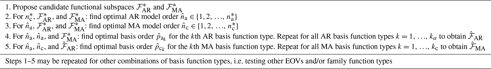
A simple backward regression scheme is employed to identify a suitable model structure, i.e. starting with high model orders, $n_{\mathrm{a}}^{*}$ and $n_{\mathrm{c}}^{*}$, and functional subspaces of high dimensionalities, ${\mathcal{F}}_{\mathrm{AR}}^{*}$ and ${\mathcal{F}}_{\mathrm{MA}}^{*}$, ensuring sufficient model complexity to capture the nonstationary response. The complexity of the initial model is then reduced in four stages: first, models with lower AR orders are estimated, and the most suitable AR order is identified. Then, the optimal MA order (given the optimal AR order) is identified in a similar fashion. The optimal basis orders for each AR and MA basis function type are identified in a similar manner. These stages are repeated for different combinations of AR and MA basis function types. The procedure is summarized in Table 1.

Table 1 Model structure identification procedure (adapted from Ebbehøj et al., 2023). High order or dimensionality is denoted by ^*.

2.5 Estimating modal parameters and their uncertainties

In this section the necessary results for estimating “frozen” modal parameters (excluding mode shapes) from an estimated GP-TARMA model and approximating the corresponding uncertainties are summarized. The frozen properties of a time-varying system represent the LTI properties at frozen time t^′; i.e. the time-varying system is represented by an infinite sequence of LTI systems (Poulimenos and Fassois, 2006). See Ebbehøj et al. (2023) for more details and also Poulimenos and Fassois (2006), Avendaño-Valencia and Fassois (2014), Spiridonakos et al. (2010), Avendaño-Valencia et al. (2017), and Yang and Lam (2019) on the computation of frozen modal parameters and their uncertainty.

The frozen modal parameters can be computed from the time-varying AR coefficients since an equivalent discrete-time state-space model with system matrix ${\mathbf{L}}_{t{}^{\prime }}$ can be formulated from the AR coefficients $\mathit{\left\{}{a}_i\right({\mathit{\xi }}_{t{}^{\prime }}):i=\mathrm{1},\mathrm{\dots },n_{\mathrm{a}}\mathit{\}}$ at each time step t^′. The first step is to compute the discrete-time eigenvalues of the eigenvalue problem:

$$\begin{array}{}\text{(19)}& {\mathbf{L}}_{t{}^{\prime }}{\mathit{v}}_i={\mathit{\rho }}_i{\mathit{v}}_i,i=\mathrm{1},\mathrm{2},\mathrm{\dots },n_{\mathrm{a}},\end{array}$$

where t^′ is the frozen-time index, and ${\mathit{v}}_i={\mathit{v}}_{i,t{}^{\prime }}$ and ${\mathit{\rho }}_i={\mathit{\rho }}_{i,t{}^{\prime }}$ are the ith right eigenvector and eigenvalue of ${\mathbf{L}}_{t{}^{\prime }}$:

$$\begin{array}{}\text{(20)}& \begin{array}{rl}& {\mathbf{L}}_{t{}^{\prime }}=\\ & {\left[\begin{array}{ccccc}\mathrm{0}& & & & \\ \mathrm{⋮}& & {\mathbf{I}}_{\left(n_{\mathrm{a}}-\mathrm{1}\right)\times \left(n_{\mathrm{a}}-\mathrm{1}\right)}& & \\ \mathrm{0}& & & & \\ -a_{n_{\mathrm{a}}}\left({\mathit{\xi }}_{t{}^{\prime }}\right)& -a_{n_{\mathrm{a}}-\mathrm{1}}\left({\mathit{\xi }}_{t{}^{\prime }}\right)& \mathrm{\cdots }& -a_{\mathrm{2}}\left({\mathit{\xi }}_{t{}^{\prime }}\right)& -a_{\mathrm{1}}\left({\mathit{\xi }}_{t{}^{\prime }}\right)\end{array}\right]}_{n_{\mathrm{a}}\times n_{\mathrm{a}}},\end{array}\end{array}$$

where I is the identity matrix with dimensions as indicated by the subscript.

The ith natural frequency $f_{i,t{}^{\prime }}$ (in Hz) and damping ratio ${\mathit{\zeta }}_{i,t{}^{\prime }}$ for frozen-time index t^′ can be computed by (Yang and Lam, 2019; Poulimenos and Fassois, 2006; Spiridonakos et al., 2010; Avendaño-Valencia et al., 2017)

$$\begin{array}{}\text{(21a)}& {\displaystyle }& {\displaystyle }{f}_{i,t{}^{\prime }}={\displaystyle \frac{\left|{\mathit{\eta }}_{i,t{}^{\prime }}\right|}{\mathrm{2}\mathit{\pi }}}\mathrm{and}{\mathit{\zeta }}_{i,t{}^{\prime }}=-{\displaystyle \frac{\mathrm{Re}\left({\mathit{\eta }}_{i,t{}^{\prime }}\right)}{\left|{\mathit{\eta }}_{i,t{}^{\prime }}\right|}},\text{(21b)}& {\displaystyle }& {\displaystyle }\mathrm{where}{\mathit{\eta }}_{i,t{}^{\prime }}=f_{\mathrm{s}}\ln \left({\mathit{\rho }}_{i,t{}^{\prime }}\right)\end{array}$$

is the equivalent ith continuous-time eigenvalue.

The uncertainty in the modal parameter estimates can be approximated by propagating the estimated AR coefficient uncertainty (quantified by ${\widehat{\mathbf{P}}}_{\mathit{\theta }}$) through the steps required to compute modal parameters from AR coefficients. These steps constitute obtaining discrete-time eigenvalues in Eq. (19), transforming the discrete-time eigenvalues to continuous-time eigenvalues in Eq. (21b), and computing the modal parameters from the continuous-time eigenvalues in Eq. (21a). The uncertainty propagation can be achieved by either Monte Carlo simulation or analytically using the first-order delta method. The former is straightforward to implement but is computationally costly, whereas the latter offers a much smaller computational burden at the price of a more elaborate implementation.

The analytic uncertainty propagation method is only valid for Gaussian PDFs with small variances. The necessary results are stated below; see Ebbehøj et al. (2023) for a brief introduction and Yang and Lam (2019) for derivations and further details. The uncertainty in the ith set of natural frequencies and damping ratios can be quantified by the following variance:

$$\begin{array}{}\text{(22)}& \begin{array}{rl}{\mathbf{\Sigma }}_{f_i,{\mathit{\zeta }}_i}=& {\displaystyle \frac{\partial {\mathit{F}}_{\mathrm{3},i}}{\partial {\mathit{\eta }}_i}}{\displaystyle \frac{\partial {\mathit{F}}_{\mathrm{2},i}}{\partial {\mathit{\rho }}_i}}{\displaystyle \frac{\partial {\mathit{F}}_{\mathrm{1},i}}{\partial \mathrm{vec}\left({\mathbf{L}}_{t{}^{\prime }}\right)}}\mathrm{vec}\left({\mathbf{P}}_{{\mathbf{L}}_{t{}^{\prime }}}\right)\\ & {\left({\displaystyle \frac{\partial {\mathit{F}}_{\mathrm{1},i}}{\partial \mathrm{vec}\left({\mathbf{L}}_{t{}^{\prime }}\right)}}\right)}^T{\left({\displaystyle \frac{\partial {\mathit{F}}_{\mathrm{2},i}}{\partial {\mathit{\rho }}_i}}\right)}^T{\left({\displaystyle \frac{\partial {\mathit{F}}_{\mathrm{3},i}}{\partial {\mathit{\eta }}_i}}\right)}^T,\end{array}\end{array}$$

where ${\mathbf{\Sigma }}_{f_i,{\mathit{\zeta }}_i}\in {\mathbb{R}}^{\mathrm{2}\times \mathrm{2}}$, vec(⋅) is the vectorization operator transforming an M×N matrix $\mathbf{A}=[{\mathit{a}}_{\mathrm{1}},{\mathit{a}}_{\mathrm{2}},\mathrm{\dots },{\mathit{a}}_N]$ to a column vector $\mathrm{vec}\left(\mathbf{A}\right)={\left[{\mathit{a}}_{\mathrm{1}}^T,{\mathit{a}}_{\mathrm{2}}^T,\mathrm{\dots },{\mathit{a}}_N^T\right]}^T\in {\mathbb{R}}^{MN\times \mathrm{1}}$, and the vectorized posterior variance matrix $\mathrm{vec}\left({\mathbf{P}}_{{\mathbf{L}}_{t{}^{\prime }}}\right)$ corresponding to ${\mathbf{L}}_{t{}^{\prime }}$ is

$$\begin{array}{}\text{(23a)}& {\displaystyle }\begin{array}{rl}& \mathrm{vec}\left({\mathbf{P}}_{{\mathbf{L}}_{t{}^{\prime }}}\right)=\mathrm{diag}\left(\mathrm{vec}\left({\mathbf{P}}_{{\mathbf{L}}_{t{}^{\prime }}}\right)\right),\end{array}\text{(23b)}& {\displaystyle }\begin{array}{rl}& \mathrm{where}{\mathbf{P}}_{{\mathbf{L}}_{t{}^{\prime }}}=\\ & {\left[\begin{array}{ccccc}& & {\mathbf{0}}_{(n_{\mathrm{a}}-\mathrm{1})\times n_{\mathrm{a}}}& & \\ {\mathit{\sigma }}_{a_{n_{\mathrm{a}}}}^{\mathrm{2}}\left({\mathit{\xi }}_{t{}^{\prime }}\right)& {\mathit{\sigma }}_{a_{n_{\mathrm{a}}-\mathrm{1}}}^{\mathrm{2}}\left({\mathit{\xi }}_{t^{\prime }}\right)& \mathrm{\cdots }& {\mathit{\sigma }}_{a_{\mathrm{2}}}^{\mathrm{2}}\left({\mathit{\xi }}_{t{}^{\prime }}\right)& {\mathit{\sigma }}_{a_{\mathrm{1}}}^{\mathrm{2}}\left({\mathit{\xi }}_{t{}^{\prime }}\right)\end{array}\right]}_{n_{\mathrm{a}}\times n_{\mathrm{a}}},\end{array}\end{array}$$

where ${\mathit{\sigma }}_{a_i}^{\mathrm{2}}\left({\mathit{\xi }}_{t{}^{\prime }}\right)=\sum _{j=\mathrm{1}}^{p_{\mathrm{a}}}{\mathit{\sigma }}_{a_{i,j}}^{\mathrm{2}}{g}_j({\mathit{\xi }}_{t{}^{\prime }}{)}^{\mathrm{2}}$, and 0 is a zero matrix with dimensions as indicated by the subscript. Note that ${\mathit{\sigma }}_{a_i}^{\mathrm{2}}\left({\mathit{\xi }}_{t{}^{\prime }}\right)$ is not necessarily Gaussian, as the individual terms of the sum can be dependent. The outputs of the three functions are

$$\begin{array}{}\text{(24a)}& {\displaystyle }& {\displaystyle }\mathit{\rho }={\mathit{F}}_{\mathrm{1}}\left(\mathrm{vec}\left({\mathbf{L}}_{t{}^{\prime }}\right)\right),\text{(24b)}& {\displaystyle }& {\displaystyle }\mathit{\eta }={\mathit{F}}_{\mathrm{2}}\left(\mathit{\rho }\right),\text{(24c)}& {\displaystyle }& {\displaystyle }\mathit{\beta }={\mathit{F}}_{\mathrm{3}}\left(\mathit{\eta }\right),\end{array}$$

where $\mathit{\rho }=[{\mathit{\rho }}_{\mathrm{1}},{\mathit{\rho }}_{\mathrm{2}},\mathrm{\dots },{\mathit{\rho }}_{n_{\mathrm{a}}}{]}^T$, $\mathit{\eta }=[{\mathit{\eta }}_{\mathrm{1}},{\mathit{\eta }}_{\mathrm{2}},\mathrm{\dots },{\mathit{\eta }}_{n_{\mathrm{a}}}{]}^T$, and $\mathit{\beta }=\mathit{\left\{}\right[f_{i,t{}^{\prime }},{\mathit{\zeta }}_{i,t{}^{\prime }}{]}^T:i=\mathrm{1},\mathrm{\dots },n_{\mathrm{a}}\mathit{\}}$. The partial derivative of F_1,i with respect to $\mathrm{vec}\left({\mathbf{L}}_{t{}^{\prime }}\right)$ is

$$\begin{array}{}\text{(25)}& \begin{array}{rl}{\displaystyle \frac{\partial {\mathit{F}}_{\mathrm{1},i}}{\partial \mathrm{vec}\left({\mathbf{L}}_{t{}^{\prime }}\right)}}=& {\left[\begin{array}{c}Re\left(\frac{\partial {\mathit{\rho }}_i}{\partial \mathrm{vec}\left({\mathbf{L}}_{t{}^{\prime }}\right)}\right)\\ Im\left(\frac{\partial {\mathit{\rho }}_i}{\partial \mathrm{vec}\left({\mathbf{L}}_{t{}^{\prime }}\right)}\right)\end{array}\right]}_{n_{\mathrm{a}}^{\mathrm{2}}\times \mathrm{1}},\\ & \mathrm{where}{\displaystyle \frac{\partial {\mathit{\rho }}_i}{\partial \mathrm{vec}\left({\mathbf{L}}_{t{}^{\prime }}\right)}}={\displaystyle \frac{{\mathit{v}}_i^T\otimes {\mathit{w}}_i^{\top }}{{\mathit{w}}_i^{\top }{\mathit{v}}_i}},\end{array}\end{array}$$

where a^⊤ denotes the complex conjugate transpose of a, ⊗ denotes Kronecker's product, and w_i is the ith left eigenvectors of ${\mathbf{L}}_{t{}^{\prime }}$ satisfying

$$\begin{array}{}\text{(26)}& {\mathit{w}}_i^{\top }{\mathbf{L}}_{t{}^{\prime }}={\mathit{\rho }}_i{\mathit{w}}_i^{\top },\end{array}$$

where w_i is a column vector. The partial derivatives of functions F_2,i and F_3,i are

$$\begin{array}{}\text{(27)}& \begin{array}{rl}{\displaystyle \frac{\partial {\mathit{F}}_{\mathrm{2},i}}{\partial {\mathit{\rho }}_i}}=& {\displaystyle \frac{\mathrm{1}}{T_{\mathrm{s}}|{\widehat{\mathit{\rho }}}_i{|}^{\mathrm{2}}}}{\left[\begin{array}{cc}\mathrm{Re}\left({\widehat{\mathit{\rho }}}_i\right)& \mathrm{Im}\left({\widehat{\mathit{\rho }}}_i\right)\\ -\mathrm{Im}\left({\widehat{\mathit{\rho }}}_i\right)& \mathrm{Re}\left({\widehat{\mathit{\rho }}}_i\right)\end{array}\right]}_{\mathrm{2}\times \mathrm{2}}\mathrm{and}\\ & {\displaystyle \frac{\partial {\mathit{F}}_{\mathrm{3},i}}{\partial {\mathit{\eta }}_i}}={\displaystyle \frac{\mathrm{1}}{\left|{\widehat{\mathit{\eta }}}_i\right|}}{\left[\begin{array}{cc}\frac{\mathrm{Re}\left({\widehat{\mathit{\eta }}}_i\right)}{\mathrm{2}\mathit{\pi }}& \frac{\mathrm{Im}\left({\widehat{\mathit{\eta }}}_i\right)}{\mathrm{2}\mathit{\pi }}\\ -\frac{\mathrm{Im}{\left({\widehat{\mathit{\eta }}}_i\right)}^{\mathrm{2}}}{|{\widehat{\mathit{\eta }}}_i{|}^{\mathrm{2}}}& \frac{\mathrm{Re}\left({\widehat{\mathit{\eta }}}_i\right)\mathrm{Im}\left({\widehat{\mathit{\eta }}}_i\right)}{|{\widehat{\mathit{\eta }}}_i{|}^{\mathrm{2}}}\end{array}\right]}_{\mathrm{2}\times \mathrm{2}},\end{array}\end{array}$$

where hats denote estimated values.

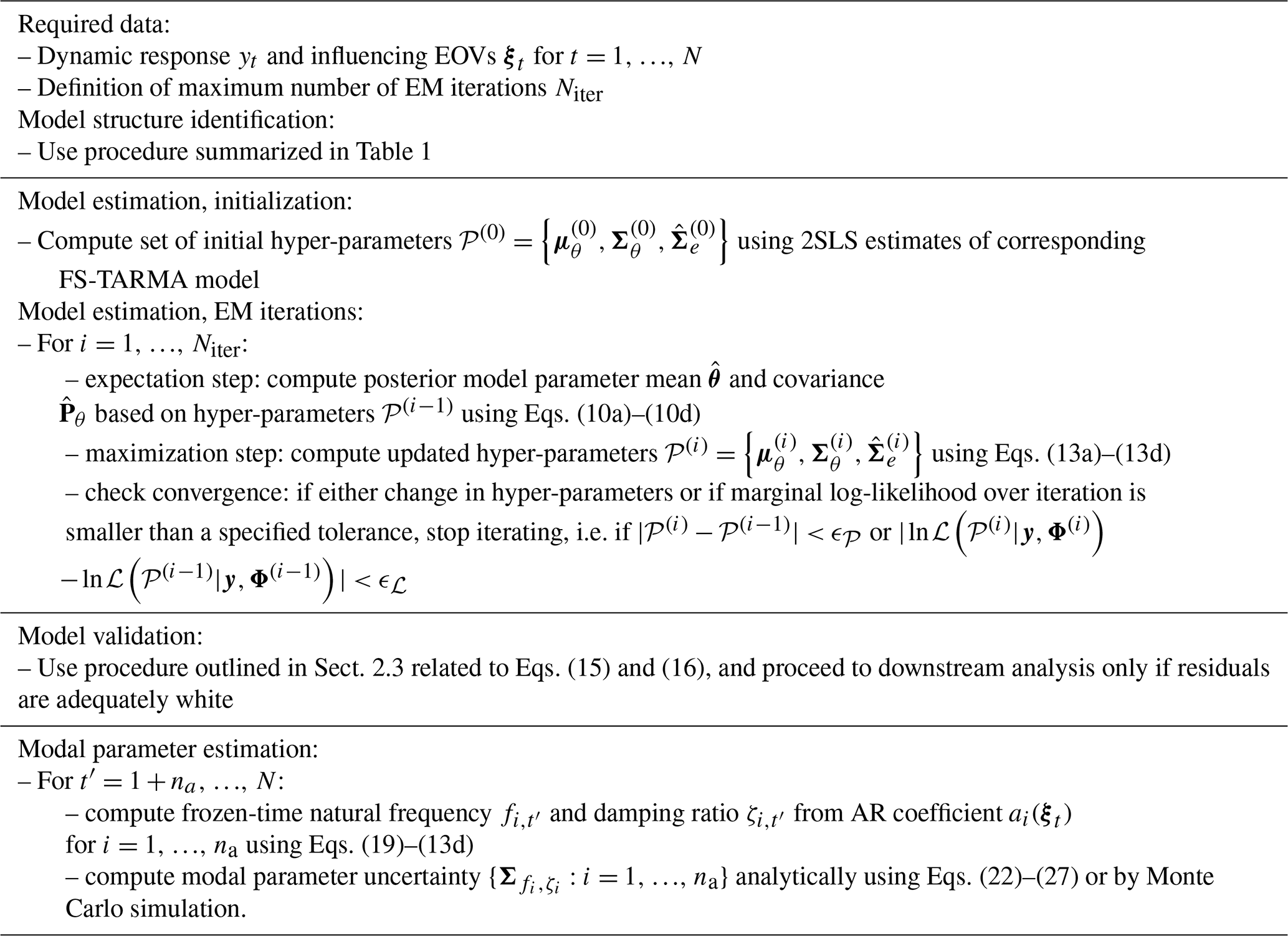
The procedure for computing natural frequencies and damping ratios and their uncertainties from AR coefficients is summarized in Table 2.

Table 2 Procedure for short-term modal parameter estimation using the GP-TARMA model (adapted from Ebbehøj et al., 2023).

2.6 Considerations for practical implementation

In this section some considerations that may be useful for the practical application of the GP-TARMA approach are listed. These are based on using the GP-TARMA model for various applications, including the wind turbine blade response of an operational wind turbine during an extreme coherent wind gust (BHawC simulation; see Ebbehøj et al., 2023), field measurements from Siemens Gamesa's fleet, and the applications in the present paper:

• Reduce bandwidth of response (output). Low-pass filter and subsequently down sample the response prior to GP-TARMA modelling such that the reduced bandwidth only contains the modes of interest; i.e. unimportant response components at higher frequencies are filtered out. This reduces the computational cost of estimating the model and may help reduce the risk of over-fitting in cases with low amounts of training data.

• Filter out high-frequency content of EOV signals by low-pass filtering. This may allow for a better fit, as modal properties usually do not vary at high frequencies (many times per second) and may prevent high-frequency noise propagating from AR coefficients to modal parameters.

• Use zero-phase filtering for low-pass filtering of response and EOV signals. Consequently, the response and EOV signals are not phase shifted by filtering.

• Add a small amount of artificial zero-mean NID noise to the (low-pass-filtered) response signal prior to GP-TARMA modelling. Adequate RMS noise levels relative to the signal are typically between 1 % and 5 %. This is an example of jittering and data augmentation in general. It can have a regularizing effect, i.e. reduce the risk of over-fitting, and is commonly used in the fields of e.g. image analysis and for machine learning methods (Iwana and Uchida, 2021; Bishop, 1995; Ding et al., 2015; Erenler and Serinagaoglu Dogrusoz, 2019). According to Bishop (1995), adding noise to training data is equivalent to Tikhonov regularization.

3 Laboratory test: shear frame structure with time-varying damping

This section presents an experimental setup of a shear frame (SF) structure with controlled time-varying damping and the experimental procedures used to generate response measurements for testing and validating the GP-TARMA approach. In Ebbehøj et al. (2023), the method is verified using responses from two simulated cases: a simple two-mode model response and an edgewise blade response during normal operation obtained with BHawC (Siemens Gamesa's in-house aeroelastic code). This section provides an experimental validation based on measurements of a simple structure conducted in a controlled setting.

3.1 Experimental setup and procedures

An experimental test rig with a three-storey SF structure was used to test modal parameter estimation methods for structures with time-varying damping. The structure has a pair of voltage-controlled electromagnetic dampers (EMDs) at each floor. Two types of tests were conducted: a base-excitation test, where the SF structure was excited with a shaker table, and a hammer test, where the structure was excited with a (measured) hammer impact. Figure 1 illustrates the experimental setup and instrumentation, and Fig. 2 shows the SF structure. The floors are quadratic ($\mathrm{110}\times \mathrm{110}\times \mathrm{10}$ mm) and are constructed from aluminium with 2 mm thick copper plate inlays at the top and bottom to increase the effect of eddy current damping through EMDs (A in Figs. 1 and 2). The beams separating the floors are $\mathrm{150}\times \mathrm{18}\times \mathrm{0.5}$ mm and are realized by four steel rulers (C), which are fixed to each floor.

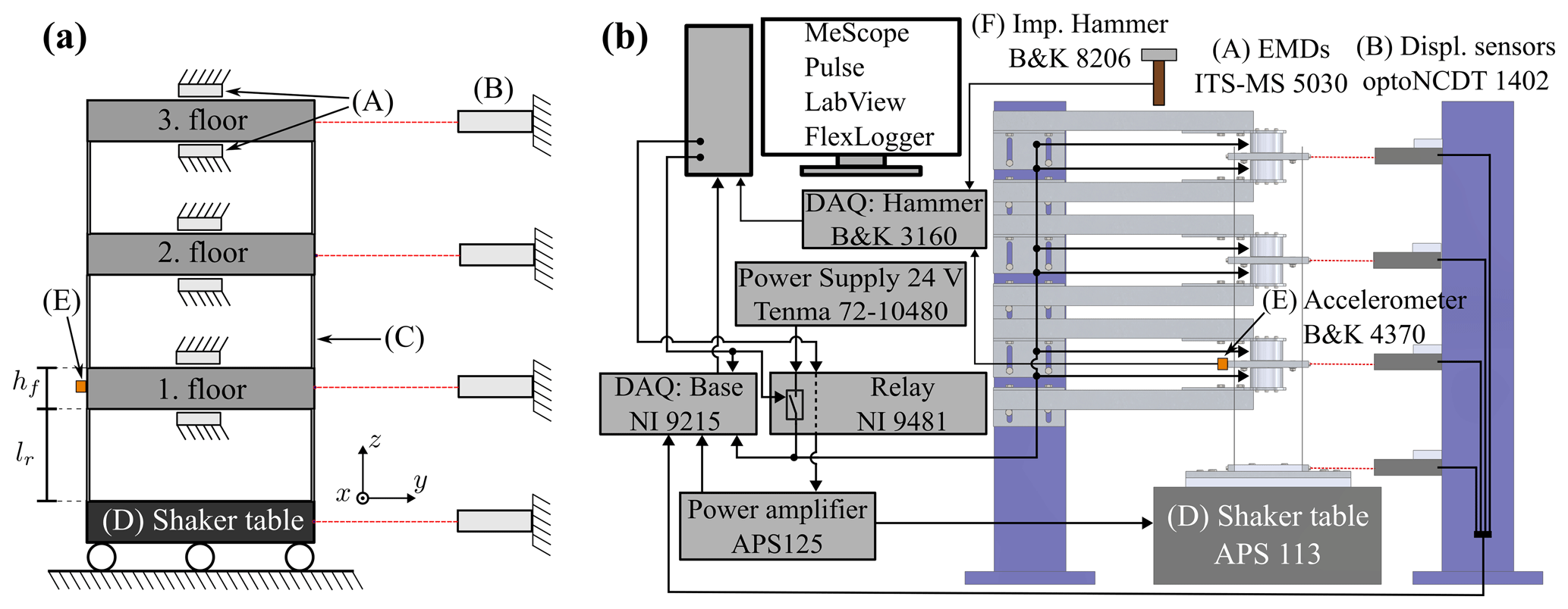
Figure 1 Experimental setup. (a) Diagram of SF structure where vibrations primarily occur in the y direction. Each floor has pairs of EMDs (A) and displacement sensors (B). Floors are separated by steel rulers (C). The entire structure is mounted on a shaker table (D). During impact hammer tests only, an accelerometer (E) is attached on the first floor. (b) Instrumentation showing the model name for each component.

Figure 2 Laboratory shear frame test setup (cf. Fig. 1, with the same annotations).

As can be seen in Fig. 1b, the shaker table (used for base-excitation tests) is driven by an amplified, digital signal using a National Instruments (NI) relay module (NI 9481) and LabView as an interface with the computer. The EMDs are powered by a 24 V signal, which is controlled in an on–off manner using the NI relay module, which is controlled using FlexLogger software. The displacement response at each floor is measured by laser displacement sensors and sampled by an NI data acquisition (DAQ) module (NI 9215) via FlexLogger, along with relevant control signals, e.g. control signals for the EMDs and amplifier.

The input signal for the shaker table used for the base-excitation test is a stochastic normally distributed broadband signal (i.e. low-pass-filtered white noise) to achieve stochastic excitation of the first three modes of the SF structure. The test is run for 60 min, all signals are collected using a sampling frequency of 50 Hz, and all EMDs are turned on and off during the test with periods of constant voltage ranging from 240 to 540 s.

For the base-excitation test, the displacement response at the third floor is used and referred to as y(t) in Sect. 3, and the measured voltage over the EMDs v(t) is used as the EOV to predict changes in damping caused by the EMDs. Figure 3 shows the displacement response y(t) and the corresponding spectrogram and spectrum, along with voltage over the EMDs v(t), indicating when the EMDs are on (24 V) and off (0 V). From the spectrum it can be seen that the first three modes have frequencies of about 1.8, 5.3, and 7.8 Hz. The measurements sampled at 50 Hz are low-pass filtered (stop band frequency of 8.05 Hz) to prevent aliasing and are subsequently downsampled to 16.67 Hz to facilitate faster estimation of the GP-TARMA model, without losing relevant information about the first three modes. In addition, artificial zero-mean NID noise with an RMS level of 1 % is added to the downsampled signal.

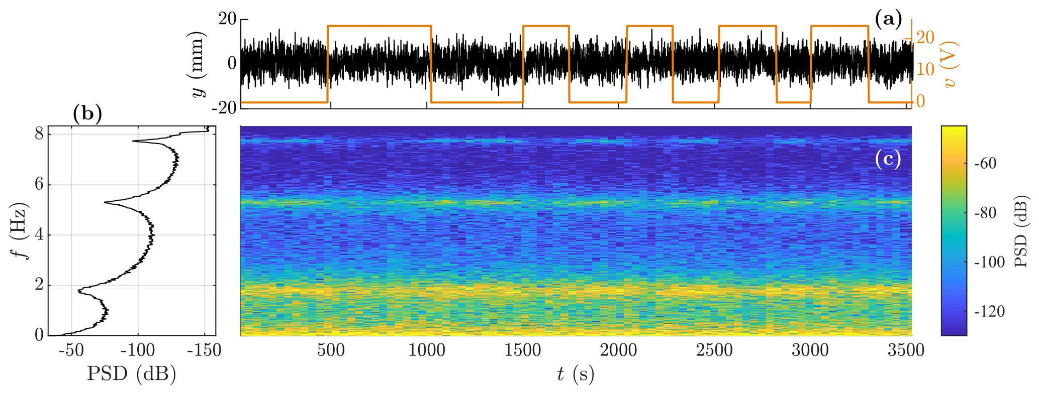
Figure 3 Measured response comprising training data for $t\in [\mathrm{0};\mathrm{2700}]$ s and test data for $t\in ]\mathrm{2700};\mathrm{3600}]$ s. (a) Displacement of the third floor y(t) (solid black line) used as the response for the analysis, overlaid by measured voltage over the electromagnetic dampers v(t) (solid orange line) used as the EOV; (b) PSD; and (c) spectrogram of y(t).

To validate modal estimates obtained from the output-only base-excitation tests, the modal parameters are also estimated by standard impact hammer tests (e.g. Ewins, 2000; Halvorsen and Brown, 1977). The instrumentation for the impact hammer tests consists of an accelerometer (E) placed on the first floor, an impact hammer with a force transducer, and a B&K 3160 front end for data acquisition. The test is conducted by impacting each floor multiple times and measuring the resulting acceleration response. The accelerometer and force transducer signals are sampled by the B&K front end and analysed using B&K Pulse and ME'scope software to estimate modal properties via local frequency response function (FRF) curve fitting. The accelerometer is only mounted on the first floor during impact hammer tests and is thus dismounted prior to base-excitation tests. During hammer tests, the shaker table is fixed. Hammer tests are conducted with all EMDs on and all EMDs off, and each test is conducted three times.

3.2 Model structure identification

A suitable model structure for modal analysis based on the third-floor response y(t) is identified using the procedure summarized in Table 1. In this controlled experimental setting, the excitation can be considered stationary since the shaker table is driven by a stationary NID signal. The functional subspace ℱ_MA representing the effect of the excitation therefore only consists of a constant-value bias vector, and the innovation variance is assumed constant (corresponding to $K=N/\mathrm{2}$ in Eq. 14). To capture the step-like damping variations caused by the EMDs turning on and off, a first-order Legendre polynomial in the voltage supplied to magnetic dampers (i.e. the EOV) is included in the functional subspace ℱ_AR, along with a constant-valued bias vector to account for the naturally occurring damping. If the voltage v(t) had changed gradually (i.e. not binary) from 0 to 24 V, ℱ_AR would likely need to include higher-order Legendre polynomials to model the voltage–damping relation. The functional subspaces for the AR and MA parts are populated as

$$\begin{array}{}\text{(28a)}& {\displaystyle }& {\displaystyle }{\mathcal{F}}_{\mathrm{AR}}=\left\{{\mathit{A}}_{\mathrm{0}},{\mathit{g}}_{\mathrm{2}}\left(\mathit{v}\right)\right\},\text{(28b)}& {\displaystyle }& {\displaystyle }{\mathcal{F}}_{\mathrm{MA}}=\left\{{\mathit{C}}_{\mathrm{0}}\right\},\end{array}$$

where ${\mathit{A}}_{\mathrm{0}}\in {\mathbb{R}}^{N\times \mathrm{1}}$ and ${\mathit{C}}_{\mathrm{0}}\in {\mathbb{R}}^{N\times \mathrm{1}}$ are constant-valued bias vectors, $\mathit{v}\in {\mathbb{R}}^{N\times \mathrm{1}}$ contains measurements of the voltage over the EMDs for times $t=\mathrm{1},\mathrm{\dots },N$, and g₂(v) is a first-order Legendre polynomial in v. The voltage signal is filtered with a centred moving average filter (better suited for step signals than regular low-pass filters) with a window width of 1 s to prevent measurement noise from propagating to the modal parameters (see Sect. 2.1).

The AR and MA model orders n_a and n_c are selected such that the predictive capabilities of the model in terms of the RSS/SSS and BIC (see Sect. 2.4) are converged, and the model captures modes of interest. In Fig. 4 RSS/SSS and BIC are seen to converge at about n_a=7 and n_c=2, constituting lower boundaries for the AR and MA model orders. The next step is to assess the model orders required to capture the modes of interest.

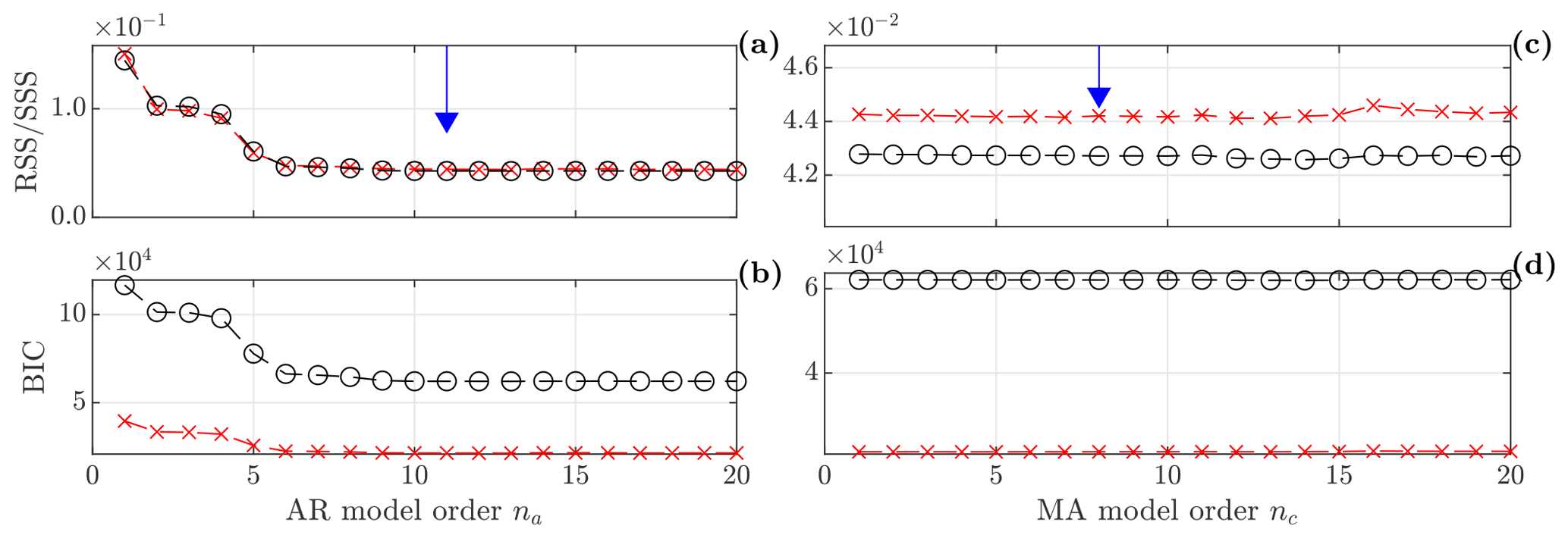
Figure 4 Model order selection measures for the training and test set (circle and red crosses) for varying AR and MA model orders. (a, c) Normalized residual sum of squares; (b, d) Bayesian information criteria. Selected model orders are marked by the blue downward-pointing arrow.

Inspecting the frequency stabilization diagram in Fig. 5, the three stable poles corresponding to the three natural frequencies of the SF can be seen to be stabilized at model orders n_a=11 and n_c=8, which are selected as the model orders used in downstream analysis. For the MA model order, the poles arguably already converge at n_c=4, but the frequency of the third mode changes slightly until fully stabilizing at n_c=8. This minor consideration can be taken because the amount of training data is large relative to the model complexity; i.e. the risk of over-fitting is small. In this case the driving model selection criterion is the ability to capture the modes of interest, as is typically the case (see Sect. 2.4).

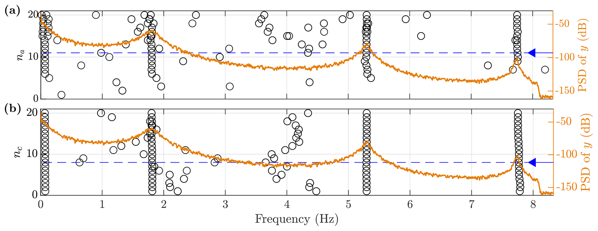
Figure 5 Frequency stabilization diagrams showing the time-averaged mean estimates of eigenfrequencies for increasing model orders, overlaid by the PSD (solid orange line) of response y. (a, b) AR and MA orders n_a and n_c. Selected model orders are indicated by the blue arrow on the left.

3.3 Model validation

In this section the model structure identified in Sect. 3.2 is validated using the procedure presented in Sect. 2.3, based on the model residual e_t $(t=\mathrm{1}+n_m,\mathrm{\dots },N)$. The standardized residual z_t and the sample ACF can be seen in Fig. 6. Judging by the time series plot, the standardized residuals for both the training and the test set appear to be stationary stochastic. This observation is supported by the ACF, for which significant correlations only exceed the 95 % confidence limits for white noise at 3 % and 4 % of the time lags (i.e. less than 5 %) for the training and test data set. Furthermore, the sign test shows that the number of sign changes in the residual sequence is well within the 95 % confidence interval of sign changes for a sequence of Gaussian white noise of the same length.

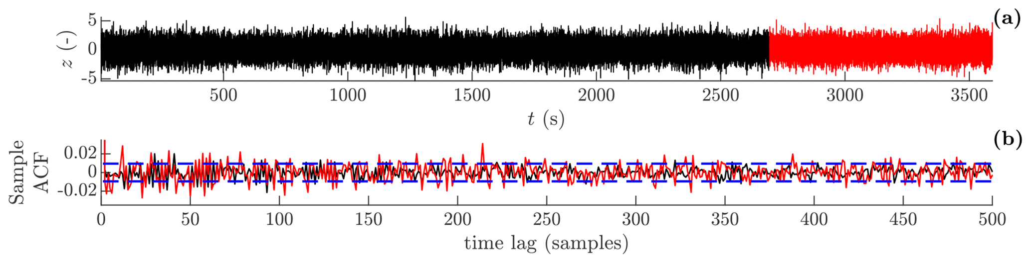
Figure 6 Residual analysis from the training and test sets (solid black line and solid red line). (a) Standardized residual z_t; (b) ACF of z_t, where the 95 % confidence interval of white noise (dashed blue line) is approximated by $\pm \mathrm{2}\sqrt{\mathrm{1}/N}$. ACF is by definition unity at lag zero but is not visible in the plot.

The above whiteness tests, based on both standardized residuals and sign changes, suggest that the present GP-TARMA model is valid and well suited for downstream analysis.

3.4 Results: modal parameter estimates

This section presents modal parameter estimates computed from the validated GP-TARMA model of the third-floor displacement response y(t) and modal parameter estimates based on hammer tests. The GP-TARMA model is estimated using 2700 s of data, corresponding to 44 820 samples (at a sampling frequency of 16.67 Hz), and about 4860, 14 310, and 21 060 oscillations of the first to third mode. Figure 7 shows the predicted response against the measured response, GP-TARMA estimates of natural frequencies and damping ratios with 95 % confidence intervals, and SSI estimates for comparison. The SSI algorithm used is correlation driven (Peeters and De Roeck, 1999; Brincker and Ventura, 2015), and the stable poles corresponding to the three modes are selected manually from frequency stabilization diagrams. The SSI estimates are also based on the displacement response of the third floor y and are computed in windows of constant voltage over the electromagnetic dampers (eight windows seen in the plot). In addition, SSI estimates based on measurements in 30 s windows are shown for the sixth and seventh windows (2043 to 2523 s).

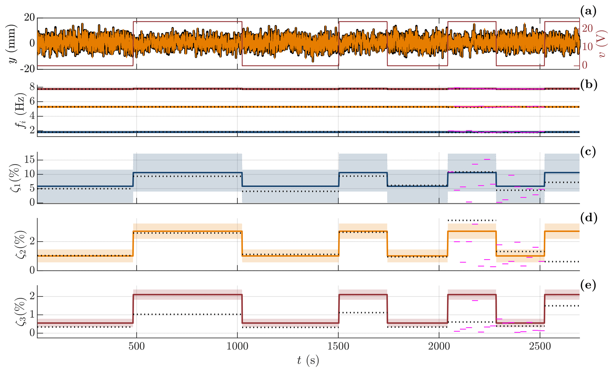
Figure 7 GP-TARMA estimates compared to SSI estimates. (a) Measured and predicted (solid black line and solid orange line) response y overlaid by voltage v over EMDs (solid red line); (b–e) GP-TARMA modal parameter estimates for the first, second, and third modes (solid blue line, solid orange line, and solid red line), where the mean estimates are shown by the solid lines, and the shaded areas indicate the estimated 95 % confidence intervals. SSI estimates for constant-voltage windows (dotted black line) and 30 s estimates (solid magenta line). (b) Natural frequency f_i; (c–e) damping ratio ζ_i of the first to third mode.

The predicted response in Fig. 7 is observed to model the measured response very well. The voltage over the electromagnetic dampers v(t) is overlaid in the plot, and 0 volt means no added damping from the electromagnetic dampers. A slight difference in response levels can be seen by comparing sections of the response with and without the electromagnetic dampers activated.

Good agreement for natural frequency estimates between GP-TARMA and SSI is observed. The modal parameter estimates are also summarized in Table 3. Furthermore, the widest confidence intervals for the GP-TARMA natural frequency estimates are ± 0.11, 0.03, and 0.02 Hz for the first, second, and third modes and seem representative of the spread of the SSI estimates, as seen in Table 3.

Table 3 Natural frequency f_i and damping ratio ζ_i estimates of the first to third mode ($i=\mathrm{1},\mathrm{2},\mathrm{3}$) for conditions with electromagnetic dampers turned off and on (0 and +) estimated with three different methods: GP-TARMA (showing mean estimates and 95 % confidence intervals, italics), SSI estimates averaged for all eight windows (excluding the 30 s estimates), and three repetitions of the hammer test.

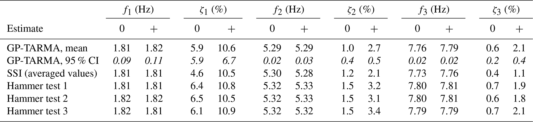
The figure and table show good agreement between SSI and GP-TARMA damping estimates, where the best agreement is observed for the second mode. The recommended minimum measurement time (Brincker and Ventura, 2015) is dictated by the third mode (with EMDs off) and is about $T_{\min }=\frac{\mathrm{10}}{f_{\mathrm{3}}{\mathit{\zeta }}_{\mathrm{3}}}=\mathrm{214}$ s (based on the hammer test estimates in Table 3); i.e. the eight constant-voltage windows of minimum 240 s should be sufficiently long for adequate SSI estimates. The GP-TARMA damping ratio estimates in Fig. 7 illustrate the idea of letting the AR coefficients, and consequently the modal parameters, be represented by EOV-dependent basis functions. In this case, the voltage over the EMDs dictates the instantaneous changes in the damping estimates. In comparison, the 30 s SSI estimates (2043 to 2523 s) are seen to be inconsistent, and many deviate considerably from the other estimates. This illustrates the need for dedicated methods for short-term damping estimation, such as the GP-TARMA approach. Using the GP-TARMA approach comes with the cost of specifying basis functions capable of representing (i.e. correlating with) the underlying causes of nonstationarity in the response, for which prior knowledge of the system is helpful. That is not needed for standard OMA methods such as SSI, although the validity of the LTI assumptions must be examined.

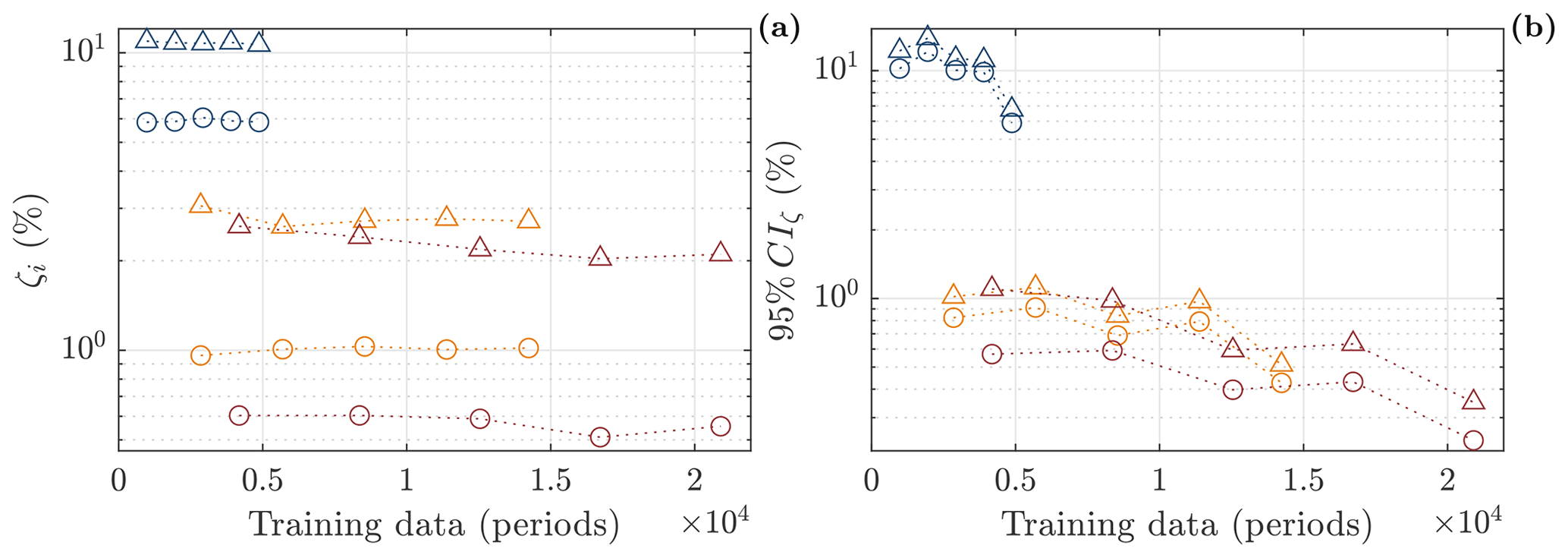
Figure 8 Convergence of damping estimates with respect to training data. (a) Mean estimates; (b) 95 % confidence interval. First, second, and third modes indicated by colour (solid blue line, solid orange line, and solid red line); estimates for electromagnetic dampers off and on (circle and triangle).

The widest damping estimate confidence intervals for the first to third mode are ± 6.7, 0.5, and 0.4 %; i.e. the damping estimate for the first mode is associated with the highest uncertainty in the three modes, as for the natural frequencies. This might reflect the fact that the training data contain more oscillation periods of the higher modes. To help elucidate this hypothesis, Fig. 8 shows the convergence of the mean damping ratio estimates and corresponding confidence intervals for all three modes in terms of oscillation periods. The results in Fig. 7 correspond to the estimates based on the largest training data set in Fig. 8. The figure indicates that only the third mode might have converged in terms of the confidence intervals, and the first mode in particular would seem to benefit from being estimated from more data. However, the mean estimates do not change much with the increase in training data. This suggests that the mean estimates might be representative despite the wide confidence intervals.

Table 3 shows that the GP-TARMA and SSI natural frequency estimates agree well with the estimates from the three hammer tests. As for the damping ratios, the three hammer test estimates compare well to the GP-TARMA and SSI estimates in the sense that they are well within the same order of magnitude. The hammer test estimates cannot be expected to agree entirely with GP-TARMA or SSI estimates because the estimates are based on data from two fundamentally different experimental tests in terms of e.g. excitation (impulse vs. stochastic), the amount of energy input, and the temporal and spatial distribution of the energy input.

The SF test results presented in this section experimentally validate the efficacy of the GP-TARMA method in providing representative short-term damping estimates and illustrate its efficacy in the short-term case compared to a traditional OMA method.

4 Full-scale wind turbine test: instability experiment

In this section the GP-TARMA approach is applied to edgewise blade response measurements. Specifically, the method is used to estimate short-term, linear equivalent modal damping of edgewise rotor modes, which are deliberately driven to flutter-like instabilities corresponding to negative damping values.

The experiments were conducted with an SWT-7.0-154 prototype wind turbine located at the DTU Wind Test Centre in Østerild, Denmark. The measurements collected in December 2018 were published by Volk et al. (2020), following up an instability field validation study (Kallesøe and Kragh, 2016). The edgewise blade modes were driven to flutter-like instabilities by momentarily allowing the rotor to run 10 % above the expected stability limit by changing the wind turbine controller parameters. As in Volk et al. (2020), the response used for the analysis is an edgewise blade bending response, obtained using a fibre Bragg optical strain sensor positioned 72 m outboard on the blade (i.e. close to the blade tip), measuring the bending response in the rotating frame of reference, which is referred to as y(t) in Sect. 4. All frequencies are normalized by the first edgewise blade frequency, and rotor speeds are normalized by the critical rotor speed of the first edgewise mode as in Volk et al. (2020).

Figure 9 shows the time series, spectrum, and spectrogram of the measured edgewise blade response y(t) along with normalized rotor speed. The figure shows a clear relation between high rotor speeds and the occurrence of “unstable” (high response levels) modes, which appear at normalized frequencies of 1.0 and 2.5. Strong response of these modes is especially prevalent at 150–230 s and 340–420 s.

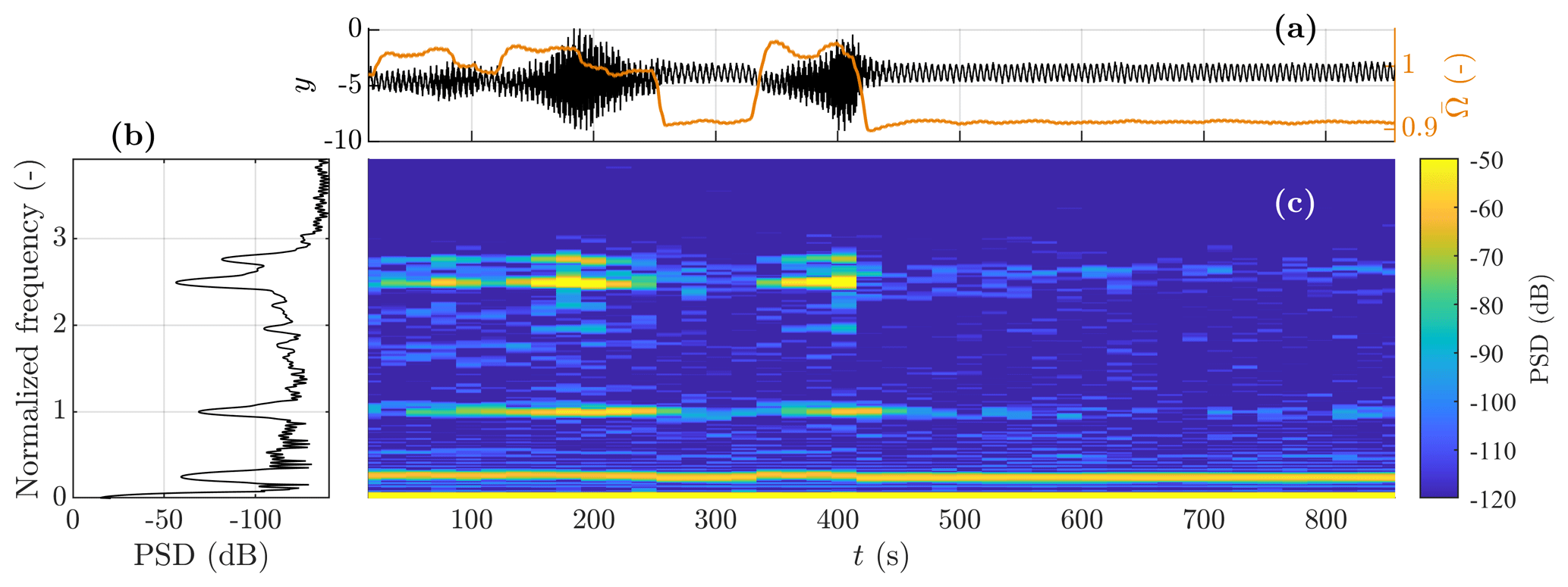
Figure 9 Measured response comprising training data for $t\in [\mathrm{0};\mathrm{665}]$ s and test data for $t\in ]\mathrm{665};\mathrm{884}]$ s. (a) Edgewise bending response y (solid black line), overlaid by normalized rotor speed $\stackrel{\mathrm{‾}}{\mathrm{\Omega }}$ (solid orange line); (b) PSD; and (c) spectrogram of edgewise bending response y(t).

The amount of available training data from this test is quite small relative to the model complexity (i.e. the number of parameters to be estimated) needed for the GP-TARMA model to represent the complex response and underlying system. The bandwidth of y(t) has therefore been reduced compared to the measurement data, and artificial zero-mean NID noise with a 5 % RMS of y(t) is added to the response y(t). These steps have been taken to use the limited measurements as efficiently as possible and to avoid over-fitting (see Sect. 2.6).

4.1 Model structure identification

The model structure is identified following the procedure in Table 1. The functional subspace ℱ_AR used to represent the AR coefficients consists of a first-order Legendre polynomial in the rotor speed Ω(t) along with a constant-valued bias vector. This allows the model to capture the effect of the varying rotor speed on the modal damping and the presumably time-invariant contribution from the structural damping. The MA coefficients are represented by harmonic functions of the azimuth angle ψ(t) to account for the nonstationary 1P effect from the changing direction of gravity in the rotating frame. Thus, the functional subspaces for the AR and MA parts are defined as

$$\begin{array}{}\text{(29a)}& {\displaystyle }& {\displaystyle }{\mathcal{F}}_{\mathrm{AR}}=\left\{{\mathit{A}}_{\mathrm{0}},{\mathit{g}}_{\mathrm{2}}\left(\mathbf{\Omega }\right)\right\},\text{(29b)}& {\displaystyle }& {\displaystyle }{\mathcal{F}}_{\mathrm{MA}}=\left\{{\mathit{C}}_{\mathrm{0}},{\mathit{h}}_{\mathrm{2}}\left(\mathit{\psi }\right),{\mathit{h}}_{\mathrm{3}}\left(\mathit{\psi }\right)\right\},\end{array}$$

where ${\mathit{A}}_{\mathrm{0}}\in {\mathbb{R}}^{N\times \mathrm{1}}$ and ${\mathit{C}}_{\mathrm{0}}\in {\mathbb{R}}^{N\times \mathrm{1}}$ are real-valued bias vectors, $\mathbf{\Omega }\in {\mathbb{R}}^{N\times \mathrm{1}}$ and $\mathit{\psi }\in {\mathbb{R}}^{N\times \mathrm{1}}$ contain rotor speed and azimuth angle measurements for $t=\mathrm{1},\mathrm{\dots },N$, g₂(Ω) is a first-order Legendre polynomial in the rotor speed Ω, and h₂(ψ)=sin (ψ) and h₃(ψ)=cos (ψ) are the harmonic functions in the azimuth angle ψ. Thus, the EOVs used in the model are the rotor speed and azimuth angle, $\mathit{\xi }=[\mathbf{\Omega },\mathit{\psi }]\in {\mathbb{R}}^{N\times \mathrm{2}}$.

Both EOVs are zero-phase low-pass filtered with a cut-off frequency of 0.3 Hz (see Sect. 2.6), and the innovation variance is estimated using Eq. (14) with a window length of 3.33 s; i.e. the GP-TARMA model can estimate damping (and natural frequency) variations down to 3.33 s. The AR (MA) model order n_a (n_c) is selected based on the predictive capability (minimizing BIC and RSS/SSS) and ability to capture the modes of interest (see Sect. 2.4), which in this case have normalized frequencies of about 1 and 2.5. As in Sect. 3.2, the model structure is dictated by the ability to capture the modes of interest; i.e. the predictive capability converges at a lower model complexity. Figure 10 shows stabilization diagrams with respect to the AR and MA orders. The selected model orders are n_a=17 and n_c=5, as these are the lowest model orders at which the poles can be considered stable. RSS/SSS and BIC converge at n_a=5 and n_c=4 (plots not included).

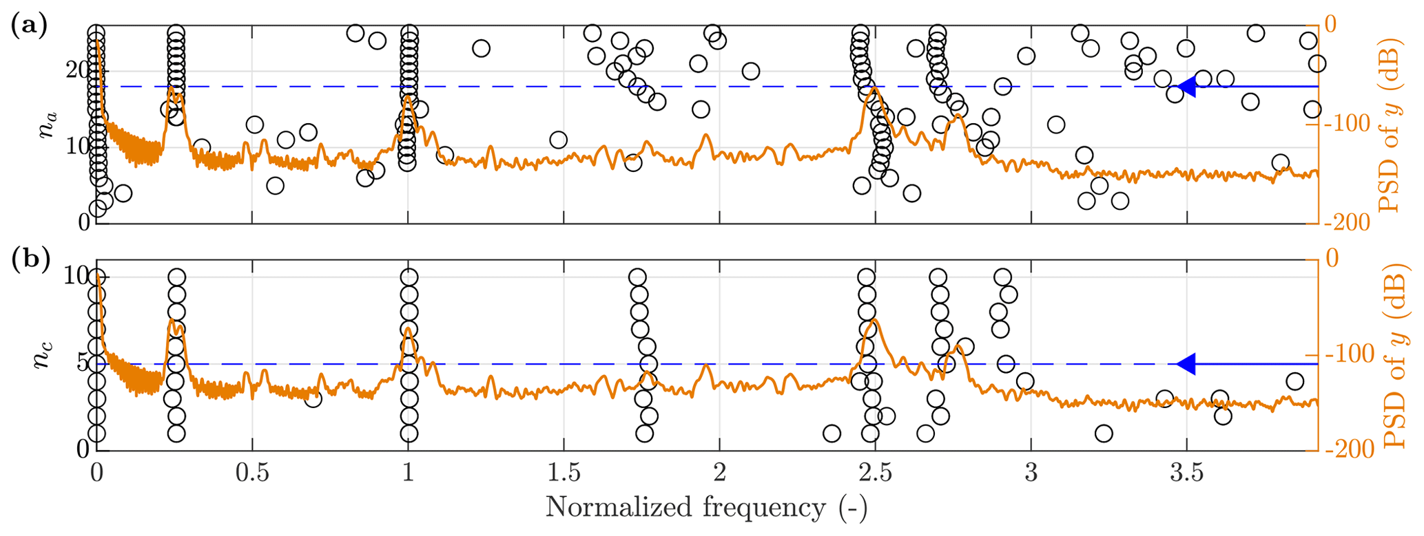
Figure 10 Frequency stabilization diagrams showing the time-averaged mean estimates of eigenfrequencies for increasing model orders, overlaid by the PSD (solid orange line) of response y. (a, b) AR and MA orders n_a and n_c. Selected model orders are marked by the blue arrows pointing to the left.

4.2 Model validation

The model structure identified in Sect. 4.1 is validated in this section, based on analysing the model residual $e_t(t=\mathrm{1}+n_m,\mathrm{\dots },N)$ as presented in Sect. 2.3. Figure 11 shows the time series, estimated ACF, and spectrum of the standardized residual z_t of the estimated GP-TARMA model with the model structure identified in Sect. 4.1. The time series of the standardized residuals for the training data does not appear as stationary white noise since the amplitude (i.e. variance) exhibits time-varying behaviour, especially at 200 and 400 s. This is because the estimated innovation variance ${\widehat{\mathit{\sigma }}}_{e,t}^{\mathrm{2}}$ is larger at those instances, which are the times of the measured instabilities. Comparing the standardized residuals for the test data to those of the training data, the time-varying behaviour is much less distinct for the test data. This can be explained by all instabilities being contained by the training set. The ACFs also indicate that the standardized residuals do not resemble white noise, as the ACFs for both the training and the test data exceed the 95 % confidence level for white noise at 13 % of the time lags. The spectrum shows a distinct peak at a normalized frequency of 0.72, which coincides with 3 times the (average) rotor speed, indicating that the model does not adequately capture the 3P effect. However, the 3P frequency is well separated from the frequencies of the modes of interest, so it is not likely to affect modal parameter estimates. The spectra of the standardized residuals for the training and test data sets can be seen to differ, as for the time series. Because the instabilities are only present in the training data, the response characteristics of the two sets are different, which limits the validity of cross-validation. In unison with the other whiteness measures, the number of sign changes in the residual sequences for the training and test data sets is not within the 95 % confidence intervals of the number of sign changes for the corresponding ideal white noise sequences. This supports the interpretation that the model residuals do not resemble white noise.

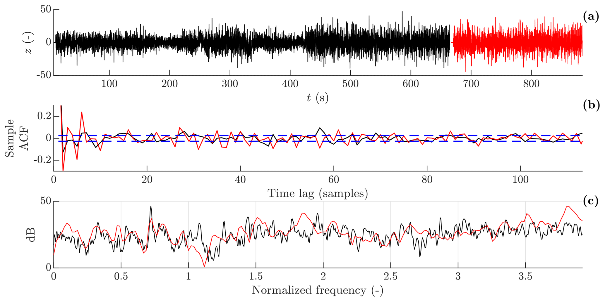
Figure 11 Residual analysis from the training and test sets (solid black line and solid red line). (a) Standardized residual z_t; (b) ACF of z_t, where the 95 % confidence interval of white noise (dashed blue line) is approximated by $\pm \mathrm{2}\sqrt{\mathrm{1}/N}$. ACF is by definition unity at lag zero but is not visible in the plot; (c) spectrum of z_t.

The residual analysis implies that the NID assumption of the innovations is violated; i.e. the model does not completely represent the statistical structure of the response. However, the frequencies at which the residuals have the largest magnitudes do not coincide with the frequencies of the two modes of interest. Thus, the modal parameters computed from the GP-TARMA based on the present data set are not expected to be entirely accurate but may still offer some insight. More available measurement data (ideally including more instability measurements) for model training could improve the model accuracy by enabling more robust and accurate model parameter estimates. In addition, a single-output model (as the actual GP-TARMA model) cannot account for the whirling effect since the frequencies of the forward- and backward-whirling modes coincide in a response measured in the rotating frame. Such model-form error might cause correlated model residuals.

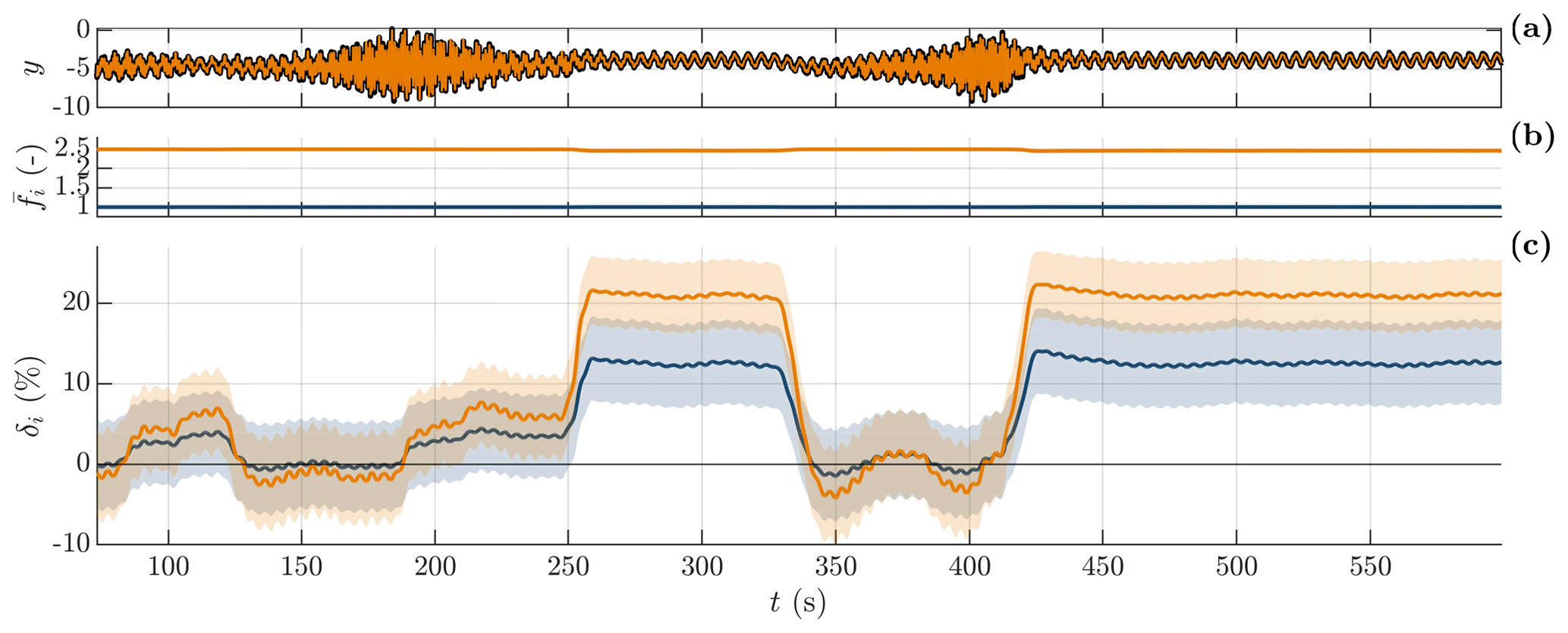
Figure 12 GP-TARMA model estimates as functions of time. (a) Measured and predicted (solid black line and solid orange line) edgewise blade response y. (b, c) Modal parameter estimates for the first and second (solid blue line and solid orange line) backward-whirling modes; the solid lines depict the mean estimates, and the shaded areas indicate 95 % confidence intervals. (b) Normalized natural frequency ${\stackrel{\mathrm{‾}}{f}}_i$. (c) Damping (logdec) δ_i.

4.3 Results: modal parameter estimates

Figure 12 shows the predicted response of the GP-TARMA model and the corresponding modal parameter estimates with uncertainties. For direct comparison to Volk et al. (2020), the damping estimates are reported in terms of the logarithmic decrement (logdec) δ, which (for small damping) is related to the damping ratio ζ by δ=2πζ. The estimated normalized frequencies correspond well with peaks in magnitude seen in the spectrum and spectrogram of response y in Fig. 9, and the average 95 % confidence intervals for the first and second modes are ± 0.01 and 0.02. Both edgewise modes can be seen to become “unstable” (i.e. negatively damped) and most noticeable between 128–187 s and 341–405 s. The time instants of the mean damping estimates crossing zero damping coincide well with the amplitude envelope changing from exponentially increasing to decreasing or vice versa; i.e. the mean damping estimates are qualitatively meaningful. The average 95 % confidence intervals of the damping estimates for the first and second modes are ± 5.2 and 4.8 % logdec, corresponding to about ± 0.8 and 0.8 % in terms of critical damping.

The uncertainty associated with damping estimates may seem considerable, as the confidence intervals cover both positive and negative damping values during the flutter-like instabilities. The uncertainty might be reduced by addressing the two limiting factors alluded to in Sect. 4.2, namely the sparse training data and the inability of the single-output GP-TARMA model to represent the whirling effect.

Figure 13 shows the damping estimates in Fig. 12 as functions of normalized rotor speed rather than time, which enables assessment of stability limits for the identified modes. The GP-TARMA estimates are plotted against two sets of damping estimates from Volk et al. (2020), consisting of experimental estimates (based on the same response data) and predictions computed using HAWCStab2 (Hansen et al., 2018) based on a numerical model of the tested wind turbine. The experimental damping estimates are obtained using logarithmic decrement fits (i.e. exponential fits of the response envelope) of bandpass-filtered (near each resonance frequency) response signals. The exponential fits are performed on four sections of the data, two sections with an exponentially increasing (negative damping) amplitude and two with an exponentially decreasing (positive damping) amplitude (see Volk et al., 2020, for details).

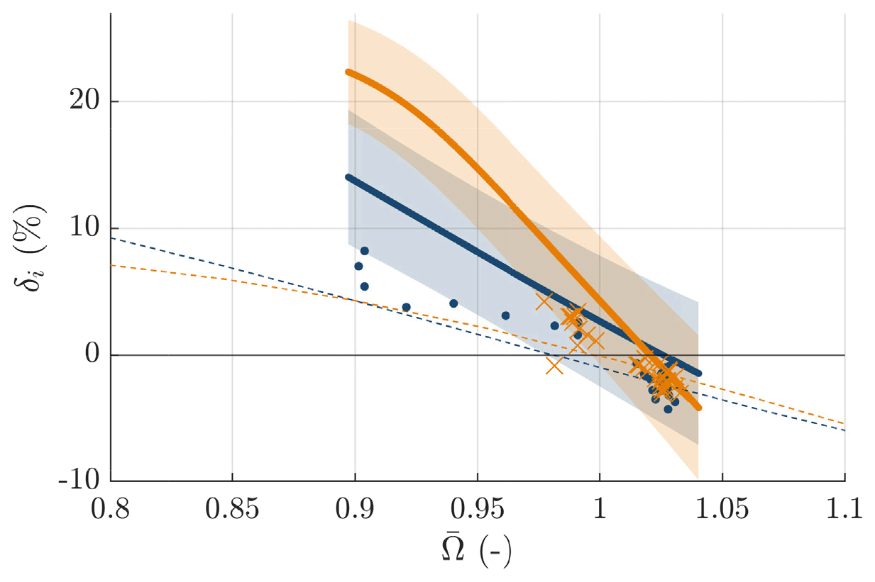
Figure 13 Modal damping of the first and second backward-whirling modes in terms of logarithmic decrement δ_i as functions of normalized rotor speed $\stackrel{\mathrm{‾}}{\mathrm{\Omega }}$. First and second backward-whirling modes: GP-TARMA (experiment) (solid blue line and solid orange line), HAWCStab2 blade only (Volk et al., 2020) (dashed blue line and dashed orange line), exponential fits (experiment) (Volk et al., 2020) (blue dot and orange cross).

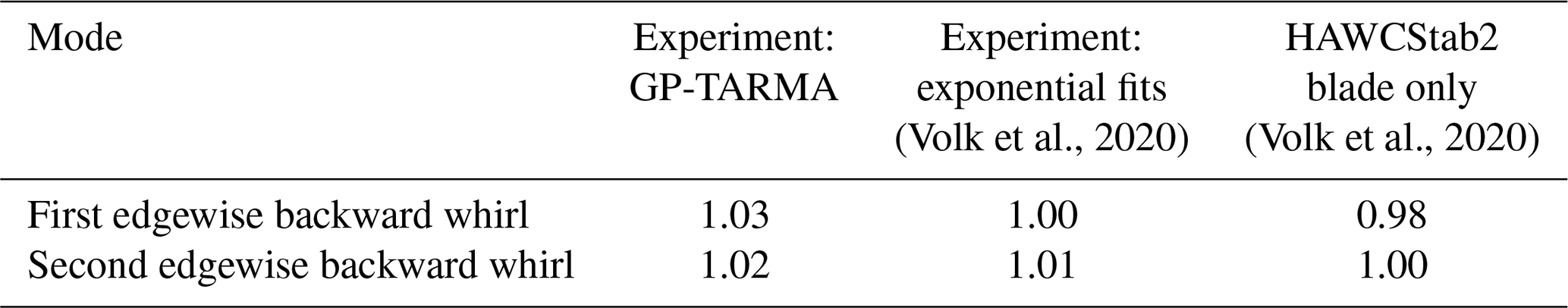
The figure shows that the GP-TARMA estimates agree quite well with the exponential fit estimates, especially near the critical rotor speeds, but the GP-TARMA damping estimates tend to be higher than the exponential fit estimates. Table 4 shows the critical rotor speed estimated by each of the three approaches. In terms of the critical rotor speed, the HAWCStab2 predictions are slightly more conservative than the two experimental results. However, comparing the ${\mathit{\delta }}_i\left(\stackrel{\mathrm{‾}}{\mathrm{\Omega }}\right)$ curve slopes in Fig. 13, the HAWCStab2 results predict less rotor speed sensitivity, i.e. are less conservative with respect to how quickly the instabilities occur. But these discrepancies are small relative to the GP-TARMA damping estimate uncertainties and the unquantified (but inevitable) uncertainties in the exponential fit estimates.

(Volk et al., 2020)(Volk et al., 2020)

Table 4 Comparison of stability limit estimates of the first and second edgewise backward-whirling modes in terms of normalized rotor speed $\stackrel{\mathrm{‾}}{\mathrm{\Omega }}$.

5 Conclusions

A recently proposed approach based on a Gaussian process time-dependent auto-regressive moving average (GP-TARMA) model for short-term damping (and natural frequency) estimation from output-only vibration response measurements for vibrating structures influenced by environmental and operational variability has been experimentally tested and validated with two distinctly different experimental setups: a laboratory shear frame structure with time-varying damping properties achieved with electromagnetic dampers and a full-scale 7 MW wind turbine prototype which was deliberately driven to flutter-like instabilities. The primary idea of the GP-TARMA approach is to condition the model parameters on measured time series of environmental and operational variables, which may enable short-term tracking of system parameters like time-varying damping and natural frequencies.

An experimental setup consisting of a shear frame structure equipped with electromagnetic dampers was presented and shown to effectively realize a system with abruptly changing damping. Short-term natural frequencies and damping ratios were estimated using the GP-TARMA model and were shown to compare well to SSI and hammer test estimates in cases where the system was time invariant. Uncertainties were observed to be larger for the first mode compared to the second and third modes, but this could be explained by the first mode being trained on effectively less training data. GP-TARMA damping estimates were compared to short-term SSI estimates based on windows of 30 s measurements. The short-term SSI estimates were observed to be inconsistent and deviating from the remaining estimates, which illustrated the effectiveness of the GP-TARMA method for short-term damping estimation relative to traditional OMA methods. The laboratory test validated the efficacy of the GP-TARMA approach in short-term damping (and natural frequency) estimation, given a sufficient amount of training data and a representative model structure.

The GP-TARMA model was also tested using edgewise blade deflection measurements from a full-scale 7 MW wind turbine prototype during a flutter test. The first and second edgewise backward-whirling modes were found to exhibit flutter-like instabilities, in agreement with a previous study. The mean damping estimates were considered qualitatively meaningful, as the GP-TARMA model predicted negative damping for two modes coinciding in time and frequency with exponentially increasing vibration amplitude. The mean damping estimates also compared quite well with estimates from a previous study obtained from the same data. The estimated stability limits, i.e. the rotor speeds at which the damping becomes zero, showed quite good agreement with a previous study. However, the model validation implied that the model residuals did not resemble white noise, meaning that the GP-TARMA model trained on the available data cannot be expected to be entirely accurate. The correlated model residuals and uncertainties of the damping estimates could potentially be reduced by training the GP-TARMA model on more data and extending the GP-TARMA model to a multiple-output model to represent whirling modes better.

The GP-TARMA approach appears to be an effective way of estimating short-term damping based on output-only measurements, given enough training data and a representative model structure. The use of GP-TARMA models for analysing transient instabilities has been showcased. SSI and other standard OMA methods are easier to implement and apply than the GP-TARMA approach since it does not require much prior knowledge of the system; i.e. these should be used for applications where the LTI assumptions are valid but may be inadequate for applications with considerable short-term EOC variability.