The rotor as a sensor – observing shear and veer from the operational data of a large wind turbine

This paper demonstrates the observation of wind shear and veer directly from the operational response of a wind turbine equipped with blade load sensors. Two independent neural-based observers, one for shear and one for veer, are first trained using a machine-learning approach and then used to produce estimates of these two wind characteristics from measured blade load harmonics. The study is based on a dataset collected at an experimental test site featuring a highly instrumented 8 MW wind turbine, an IEC-compliant (International Electrotechnical Commission) met mast, and a vertical profiling lidar reaching above the rotor top.

The present study reports the first demonstration of the measurement of wind veer with this technology and the first validation of shear and veer with respect to lidar measurements spanning the whole rotor height. Results are presented in terms of correlations, exemplary time histories, and aggregated statistical metrics. Measurements of shear and veer produced by the observers are very similar to the ones obtained with the widely adopted profiling lidar while avoiding its complexity and associated costs.

1 Introduction

The goal of this paper is to demonstrate the observation of wind shear and veer directly from the operational response of a wind turbine. This is achieved by the concept of the rotor as a sensor, where the blades scanning the flow field are used to measure relevant characteristics of the inflow. A key advantage of this approach, called wind sensing, is that it does not require extra hardware but simply relies on the standard operational data available in the supervisory control and data acquisition (SCADA) system in addition to blade load measurements. Although the latter are not always available on all production turbines, they are becoming more and more widespread as they are used for other functions such as load mitigation and condition monitoring.

A novelty of this paper is that it is the first ever demonstration – to the authors' knowledge – of the observation of veer using this technology. This is made possible by the formulation recently proposed by Kim et al. (2023), where feed-forward neural networks are trained to estimate various wind characteristics from blade load harmonics. This machine-learning approach improves on various previous formulations based on the use of load harmonics, starting with the study of Bottasso and Riboldi (2014) and then further developed over the years, as more completely described in Bertelè et al. (2021) and references therein. In addition to vertical shear and veer, load harmonics can be used to estimate horizontal shear and directions (lateral misalignment and upflow). However, load harmonics are not the only way to estimate wind inflow characteristics. For example, Bottasso et al. (2018) used the rotor blades as local scanning wind sensors, which produce estimates of the vertical and horizontal shear, the latter serving also as a wake detector (Schreiber et al., 2020).

A second novelty of the paper is the demonstration of the observation of shear (and veer) over the entire rotor disk. Although the field validation of shear has been reported before, previous studies were based on measurements from met masts reaching only up to hub height (Bertelè et al., 2021; Schreiber et al., 2020) and not to the top of the rotor. The present work is based on the Bremerhaven (BHV) test site (Meyer and Gottschall, 2022), which features a large 8 MW AD8-180 wind turbine. In the framework of unrelated projects, the turbine was equipped with various sensors that include optical strain gauges along the blades (Wegner et al., 2022). The site is complemented by an IEC-compliant (International Electrotechnical Commission) met mast and by a vertical-profiling pulsed scanning lidar capable of reaching well above the rotor top.

Results reported in this paper indicate that both shear and veer can be measured by wind sensing, in general exhibiting a very good match with the corresponding measurements provided by the vertical profiling (VP) lidar, an IEC-approved and widely adopted device for resource assessment and power performance testing (IEC, 2022). This is remarkable because when load sensors are already installed on a turbine, the measurement of these inflow quantities comes at no additional hardware purchase or maintenance cost, as the technology simply amounts to an onboard software upgrade.

Most turbines today operate based only on a very limited knowledge of the ambient conditions as provided by the onboard anemometry system. Although this is the current standard, it is reasonable to expect that a more complete knowledge of the inflow might improve the way future turbines will be operated. As an example, the control of wakes might benefit from improved knowledge of the inflow (Meyers et al., 2022). In fact, various studies have investigated and clarified the effects of shear (Fleming et al., 2014; Vollmer et al., 2016; Gebraad et al., 2016; Bromm et al., 2017) and veer (Vollmer et al., 2016) on wake path and recovery. When the effects of shear and veer on wakes are of a similar order of magnitude as the ones caused by the control action (e.g., an intentional yaw misalignment), neglecting their presence will lead to a loss of performance. The shear and veer observers demonstrated here could inform a park controller of the inflow conditions at the rotor disk of each turbine in a farm (in contrast to a met mast, which will never be exactly co-located with a turbine and will only rarely be exactly in front of it) at essentially no cost and with no extra hardware (in contrast to lidar-based solutions).

The paper is organized in two main parts. First, Sect. 2 presents the methods. Section 2.1 reviews the formulation of the shear and veer observers following the approach developed by Kim et al. (2023). Next, Sect. 2.2 describes the BHV test site and its instrumentation. Finally, Sect. 2.3 describes the calculation of shear and veer from the lidar and mast measurements. This first methodological section is followed by Sect. 3, which presents the results. First, Sect. 3.1 discusses the training of the neural-based observers on a portion of the dataset. Next, Sect. 3.2 provides an analysis of their performance on an independent validation dataset, considering correlations between estimates and lidar-provided references, an exemplary time history, and aggregated statistical quality metrics. Finally, Sect. 4 concludes this work discussing the main findings.

2 Methods

2.1 Formulation of the shear and veer observers

Following Kim et al. (2023), the wind observer is formulated as

$$\begin{array}{}\text{(1)}& y_{\mathrm{E}}=\mathrm{NN}(\mathit{p},{\mathit{x}}_{\mathrm{M}}),\end{array}$$

where y represents a scalar wind characteristic; $\mathrm{NN}(\cdot ,\cdot )$ is a single-output neural network (Bishop, 2006) with free parameters p; x is the vector of N_x network inputs; and (⋅)_E and (⋅)_M indicate estimated and measured quantities, respectively. In this work, two separate networks are considered: one for vertical linear wind shear κ_v and one for vertical linear wind veer Δθ¹.

Considering a single-hidden-layer feed-forward neural network with M hidden neurons, function $\mathrm{NN}(\cdot ,\cdot )$ is written as

$$\begin{array}{}\text{(2)}& \mathrm{NN}(\mathit{p},\mathit{x})={\mathit{w}}^T\mathit{\sigma }({\mathbf{V}}^T\mathit{x}+\mathit{a})+b,\end{array}$$

where σ(⋅) is a vector of sigmoid activation functions, V_ij and a_i are the synaptic weights and biases connecting the input layer with the hidden layer, while w_i and b connect the hidden layer with the output scalar y, with $i=[\mathrm{1},M]$ and $j=[\mathrm{1},N_x]$. These free model parameters are stored in vector $\mathit{p}=\mathit{\{}\mathrm{\dots },w_j,\mathrm{\dots },V_{ij},\mathrm{\dots },a_i,\mathrm{\dots },b{\mathit{\}}}^T$.

The free network parameters p are trained by backpropagation to minimize the error cost function

$$\begin{array}{}\text{(3)}& E\left(\mathit{p}\right)={\displaystyle \frac{\mathrm{1}}{N}}\sum _{l=\mathrm{1}}^N{\left(y_{{\mathrm{E}}_l}(\mathit{p},{\mathit{x}}_{{\mathrm{M}}_l})-y_{{\mathrm{M}}_l}\right)}^{\mathrm{2}}+W{\displaystyle \frac{\mathrm{1}}{N_p}}\sum _{m=\mathrm{1}}^{N_p}{p}_m^{\mathrm{2}},\end{array}$$

where $N_p=M(N_x+\mathrm{2})+\mathrm{1}$. The first term of the objective function drives the estimates $y_{{\mathrm{E}}_l}$ produced by the network towards the N available measurements $y_{{\mathrm{M}}_l}$. The second term of the objective is a Bayesian regularization, which reduces the chances of being trapped in local minima (Burden and Winkler, 2009). The tunable coefficient W sets the relative weight of the Bayesian and error terms. The unknown network weights are iteratively corrected as $\mathrm{\Delta }\mathit{p}=-\mathit{\eta }\partial E\left(\mathit{p}\right)/\partial \mathit{p}$, where η is the learning rate. The implementation of the neural network and its training is based on the MATLAB Deep Learning Toolbox (Matlab, 2023).

The network input vector is defined as

$$\begin{array}{}\text{(4)}& \mathit{x}=\mathit{\{}{\mathit{m}}^T,V,\mathit{\rho }{\mathit{\}}}^T,\end{array}$$

where m is a vector of blade load harmonics, V is wind speed, and ρ is air density. The presence of wind speed V among the inputs accounts for the different behavior, control, and deformation of the wind turbine in different operating conditions. This scheduling wind speed is computed as a 30 s moving average of the estimated rotor-effective wind speed (Soltani et al., 2013). The dependency on air density ρ accounts for the aerodynamic origin of the loads; further details are available in Kim et al. (2023).

Harmonics are computed for the out- and in-plane load components denoted (⋅)^OP and (⋅)^IP, respectively, from the corresponding strain gauge signals via the Coleman–Feingold transformation (Coleman and Feingold, 1958) and then filtered to remove any remaining spurious noise. Following the analysis developed in Kim et al. (2023), only once-per-revolution (1P) harmonics are used for the vertical linear shear case, and vector m is defined as

$$\begin{array}{}\text{(5)}& \mathit{m}={\left\{m_{\mathrm{1}\text{c}}^{\mathrm{OP}},m_{\mathrm{1}\text{s}}^{\mathrm{OP}},m_{\mathrm{1}\text{c}}^{\mathrm{IP}},m_{\mathrm{1}\text{s}}^{\mathrm{IP}}\right\}}^T.\end{array}$$

On the other hand, the estimation of linear veer requires a richer input also including the twice-per-revolution (2P) harmonics, leading to the following definition of vector m:

$$\begin{array}{}\text{(6)}& \mathit{m}={\left\{m_{\mathrm{1}\text{c}}^{\mathrm{OP}},m_{\mathrm{1}\text{s}}^{\mathrm{OP}},m_{\mathrm{1}\text{c}}^{\mathrm{IP}},m_{\mathrm{1}\text{s}}^{\mathrm{IP}},m_{\mathrm{2}\text{c}}^{\mathrm{OP}},m_{\mathrm{2}\text{s}}^{\mathrm{OP}},m_{\mathrm{2}\text{c}}^{\mathrm{IP}},m_{\mathrm{2}\text{s}}^{\mathrm{IP}}\right\}}^T.\end{array}$$

In the previous expressions, subscripts (⋅)_ks and (⋅)_kc indicate kP sine and cosine harmonic amplitudes, respectively. A simple explanation of the harmonic content of the shear and veer observers is offered in Appendix A. Kim et al. (2023) offer a more detailed analysis of the relationship between inflow characteristics and harmonic content of the loads. The analysis developed there can be used to estimate the number of harmonics that is theoretically necessary in order to resolve a desired polynomial order in the shear and veer.

Both the simple analysis in Appendix A and the more refined one in Kim et al. (2023) indicate that veer can be estimated based only on 2P harmonics. However, it was verified that an implementation based on both the 1P and 2P harmonics provides slightly more precise estimates; the results shown later are therefore based on the 1P–2P implementation. The reason for this apparent discrepancy might be due to the approximate nature of the theoretical analysis, which is based on a number of simplifying assumptions.

Limiting the observer to the 1P and 2P harmonics has potential advantages over more complex implementations. First, higher harmonics are associated with higher-order variations in the inflow characteristics, which may be affected by the fast and small eddies in the flow caused by turbulence. Conversely, more slowly varying inflow characteristics are mostly driven by changes in the stability of the atmosphere, which in turn drives wake path and recovery. If the goal of the observer is to inform a wind farm controller, these latter, slower effects are of interest, whereas the former fast disturbances should be rejected (Meyers et al., 2022). Additionally, it is reasonable to assume that the lower harmonics between two turbines of the same type implementing the same controller will be similar, whereas higher harmonics might exhibit some increased turbine-to-turbine variability. Therefore, limiting the use to solely 1P and 2P harmonics might make it possible to train the observers on a machine and then use it on another (of the exact same type), although there is not yet any direct proof of this assertion.

A graphical depiction of the neural observers for shear and veer is reported in Fig. 1a and b, respectively.

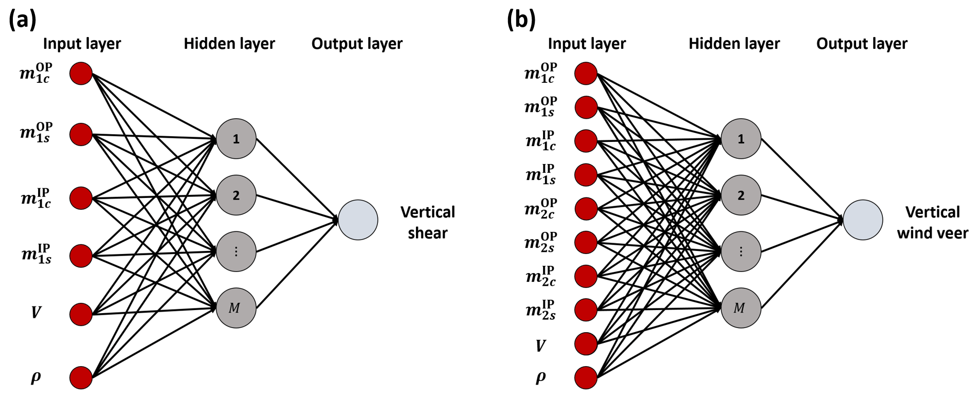
Figure 1 Graphical representation of the neural observers of vertical wind shear (a) and vertical wind veer (b), with their respective inputs.

2.2 Test site

The shear and veer observers were identified and validated using wind field and turbine load measurements from the BHV test site (Meyer and Gottschall, 2022), a former airport located in close proximity to Bremerhaven in the northwest of Germany next to the Weser river. The test site is built around the 8 MW research wind turbine AD8-180. Flat and homogeneous terrain conditions are present in the westerly direction, whereas urban terrain prevails in the easterly direction. Various wind- and turbine-related measurements have already been carried out at this site, as reported in previously published studies (Giyanani et al., 2022; Huhn and Gómez-Mejía, 2022; Meyer and Gottschall, 2022; Hung et al., 2022; Wegner et al., 2022). The test site is shown in Fig. 2, with a view looking east.

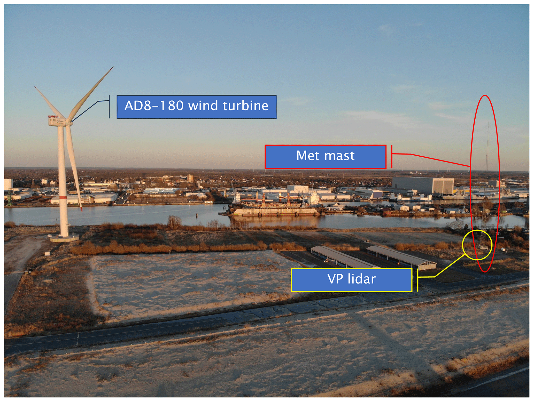
Figure 2 View of the BHV test site from west to east, with the AD8-180 wind turbine on the left and the met mast and VP lidar on the right.

The AD8-180, an 8 MW machine with a 180 m rotor diameter (D) and a 115 m hub height, is equipped with several sensors including strain gauges placed at various spanwise positions along the blades. Operational data from the SCADA system, together with the strain gauge measurements, are available at a 25 Hz frequency. Flapwise and edgewise measurements from the strain gauges placed at blade root were converted into out- and in-plane components based on blade pitch angle. Next, using the azimuthal rotor position, the load signals were converted into 1P and 2P harmonics to be used as network inputs (see Eq. 4).

An IEC-compliant met mast is installed at a distance of 399.3 m (≈ 2.2 D) from the turbine in the 189° direction. The mast is equipped with cup anemometers at five heights up to 114.7 m, as well as wind vanes at three heights reaching up to 110 m, i.e., just below the hub. Data from the mast are available at a sampling rate of 1 Hz. Additionally, a barometer, thermometer, and hygrometer are available to derive air density.

A VP lidar of the type WindCube V2 is installed next to the met mast, measuring wind speed and direction at heights from 40 m up to 290 m. Various studies have shown good agreement between cup anemometers and VP lidars for the measurement of wind speed and direction (Gottschall et al., 2012; Clifton et al., 2018). Furthermore, the VP lidar is an established measurement device for power performance testing and wind resource assessment according to IEC 61400-50-2:2022 (IEC, 2022). The lidar sequentially measures line-of-sight velocities for a fixed scan pattern of four beams along a cone with a half-opening angle of 28° combined with one vertically scanning beam. Wind speed and direction are then reconstructed at each measured height from the line-of-sight velocities with every updated line-of-sight measurement, i.e., every 0.8 s. As the met mast provides wind speed and direction measurements only for the lower half of the rotor, the VP lidar is used to measure these quantities from a height of 40 m to the top of the rotor.

A sketch of the relevant heights and distances of turbine, met mast, and lidar are shown in Fig. 3. This study is based on a dataset of synchronized turbine, mast, and lidar measurements collected for 115 d within the period from 30 July to 12 December 2021. The dataset contains significant variability in ambient conditions and frequent occurrence of southerly winds, where the met mast is directly upwind of the turbine.

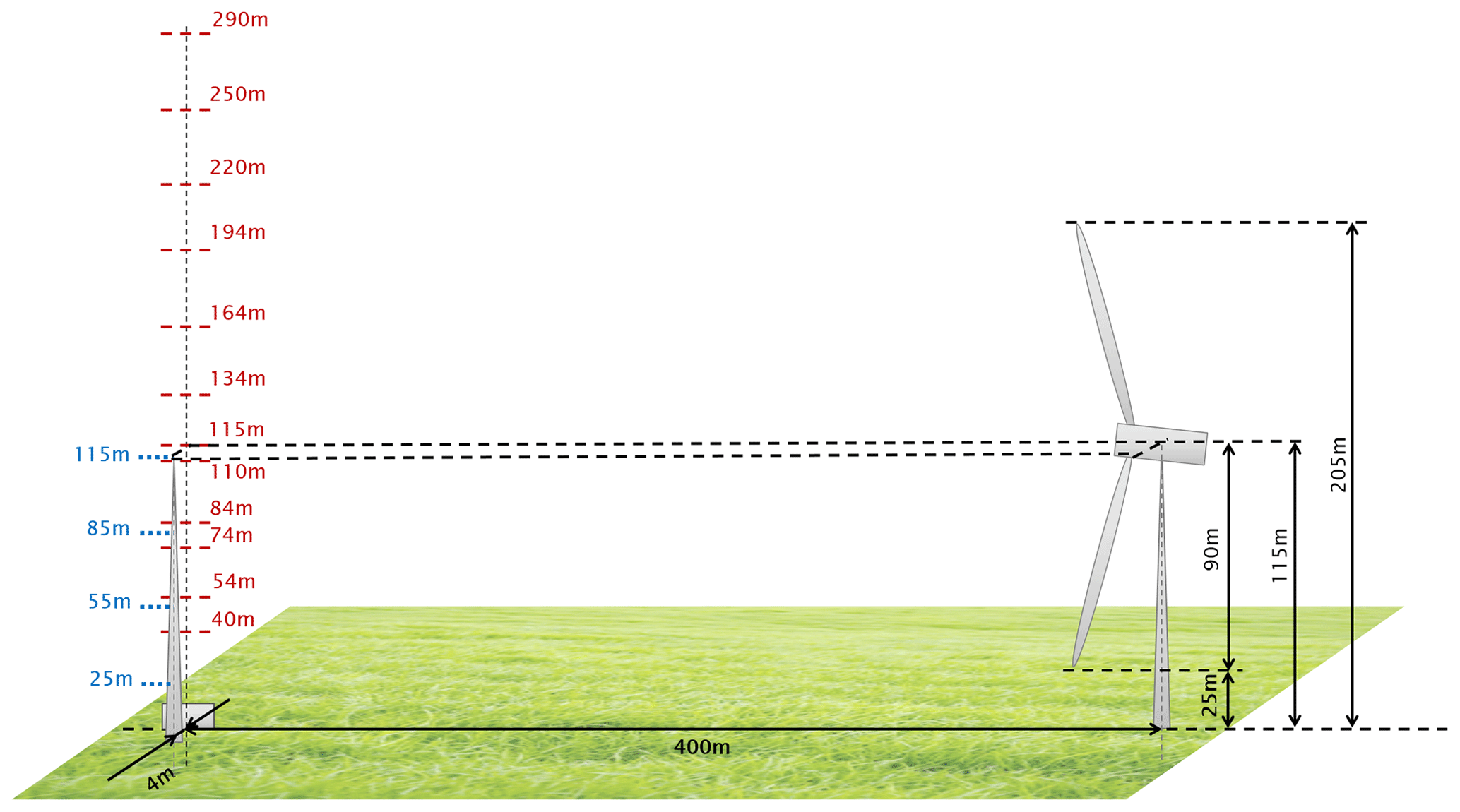
Figure 3 Sketch (to scale) of the test site with the relevant dimensions rounded to the next integer. Heights are given relative to ground level at the turbine location. Blue labels – met mast measurement heights; red labels – lidar measurement heights.

2.3 Field measurements of shear and veer

The wind observer networks are trained based on measurements of the wind shear and veer together with their corresponding network inputs, as expressed in the first term of the objective function given by Eq. (3).

In this paper, wind shear and veer measurements were provided by the VP lidar. In fact, this instrument measures at 12 heights from 40 to 290 m above ground, thus including most of the rotor-swept area, which ranges from the lower blade tip (LBT) point z_LBT=25 m to the higher blade tip (HBT) point z_HBT=205 m.

For both shear and veer, a linear best fit was first computed using the nine VP lidar measurements of wind speed V and direction Γ included within the rotor-swept area, i.e., between 40 and 195 m above ground (see Fig. 3). Next, shear and veer were computed as

$$\begin{array}{}\text{(7a)}& {\displaystyle }{\mathit{\kappa }}_{\mathrm{v}}={\displaystyle \frac{V\left(z_{\mathrm{HBT}}\right)-V\left(z_{\mathrm{LBT}}\right)}{z_{\mathrm{HBT}}-z_{\mathrm{LBT}}}},\text{(7b)}& {\displaystyle }\mathrm{\Delta }\mathit{\theta }={\displaystyle \frac{\mathrm{\Gamma }\left(z_{\mathrm{HBT}}\right)-\mathrm{\Gamma }\left(z_{\mathrm{LBT}}\right)}{z_{\mathrm{HBT}}-z_{\mathrm{LBT}}}},\end{array}$$

where the terms at the numerators of these two expressions are computed via the linear fit evaluated at the lower and higher blade tip points, respectively.

Before using these lidar-based rotor-effective wind characteristics for training, their accuracy was verified against the IEC-compliant met mast present at the site. Vertical shear and veer were derived from the mast measurements following the same linear-fitting procedure previously described for the lidar, i.e., using

$$\begin{array}{}\text{(8a)}& {\displaystyle }{\mathit{\kappa }}_{\mathrm{v}\mathrm{Low}}={\displaystyle \frac{V\left(z_{\mathrm{HUB}}\right)-V\left(z_{\mathrm{LBT}}\right)}{z_{\mathrm{HUB}}-z_{\mathrm{LBT}}}},\text{(8b)}& {\displaystyle }\mathrm{\Delta }{\mathit{\theta }}_{\mathrm{Low}}={\displaystyle \frac{\mathrm{\Gamma }\left(z_{\mathrm{HUB}}\right)-\mathrm{\Gamma }\left(z_{\mathrm{LBT}}\right)}{z_{\mathrm{HUB}}-z_{\mathrm{LBT}}}}.\end{array}$$

Note that since the mast reaches only up to hub height z_HUB, the resulting shear and veer are defined only over the lower half of the rotor disk.

To perform a valid comparison, the shear and veer derived from the lidar were also computed over the lower part of the rotor, which was obtained by considering only measurements in the range from 40 to 115 m. Figure 4 shows the results of this comparison in the form of 10 min averages, reporting the met mast measurements on the x axis and the corresponding lidar quantities on the y axis. Wind speeds at hub height, shown in Fig. 4a, have a high Pearson coefficient R of 0.99 and a mean absolute error (MAE) of about 0.122 m s⁻¹. There is a high correlation also for wind shear and veer, which have Pearson coefficients of 0.97 and 0.95, respectively, as shown in Fig. 4b and c. In addition to the different measurement technologies, differences might be caused by the fact that the mast reaches down to 25 m above the terrain, whereas the lowest measurement point for the lidar is at 40 m. Figure 4c suggests the existence of a slight slope difference for veer. This might be caused by the met mast because vertical veer is obtained from only two heights above ground and possibly because of some minor misalignment of its wind direction sensors. Given its uncertain origin, lidar measurements were not recalibrated to eliminate this effect.

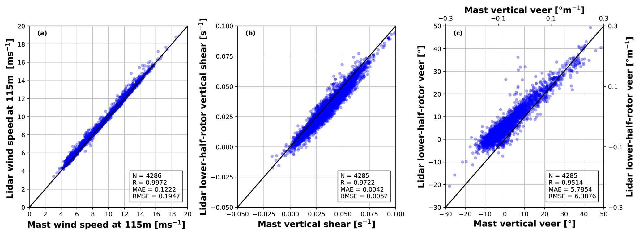
Figure 4 Correlation of 10 min averages of measured quantities from the met mast (x axis) and VP lidar (y axis). Hub-height wind speed (a); lower-half-rotor vertical shear (b); and lower-half-rotor veer, in both absolute terms (°; i.e., between z_LBT and z_HUB) and relative (° m⁻¹) terms (c). Solid black line – ideal match; R – Pearson’s correlation coefficient; N – number of data points; MAE – mean absolute error; and RMSE – root mean square error.

3 Results

The wind observers for shear and veer formulated in Sect. 2.1 were tested on a dataset collected at the site described in Sect. 2.2. First, in Sect. 3.1 we explain the identification of the observers from a subset of the data. Next, Sect. 3.2 presents the results obtained using the observers on an independent validation subset.

3.1 Observer identification

The dataset was cleaned to retain only data points when the turbine was operational and all necessary measurements (SCADA, strain gauges, and lidar) were available. This resulted in about 18 full days of valid data points spread between August and December. The training subset was obtained by picking a random 67 % of the data points (i.e., about 290 h) within the whole set to exclude effects due to seasonal variability. The remaining set (i.e., about 138 h) was used for validation. Although in principle the observer could be trained directly on high-frequency data, following the example of Kim et al. (2023) 10 min averages were preferred in order to mitigate the effects of possible outliers. The ranges and number of occurrences of values of wind speed V, air density ρ, vertical shear κ_v, and veer Δθ in the two data sets are shown in Fig. 5.

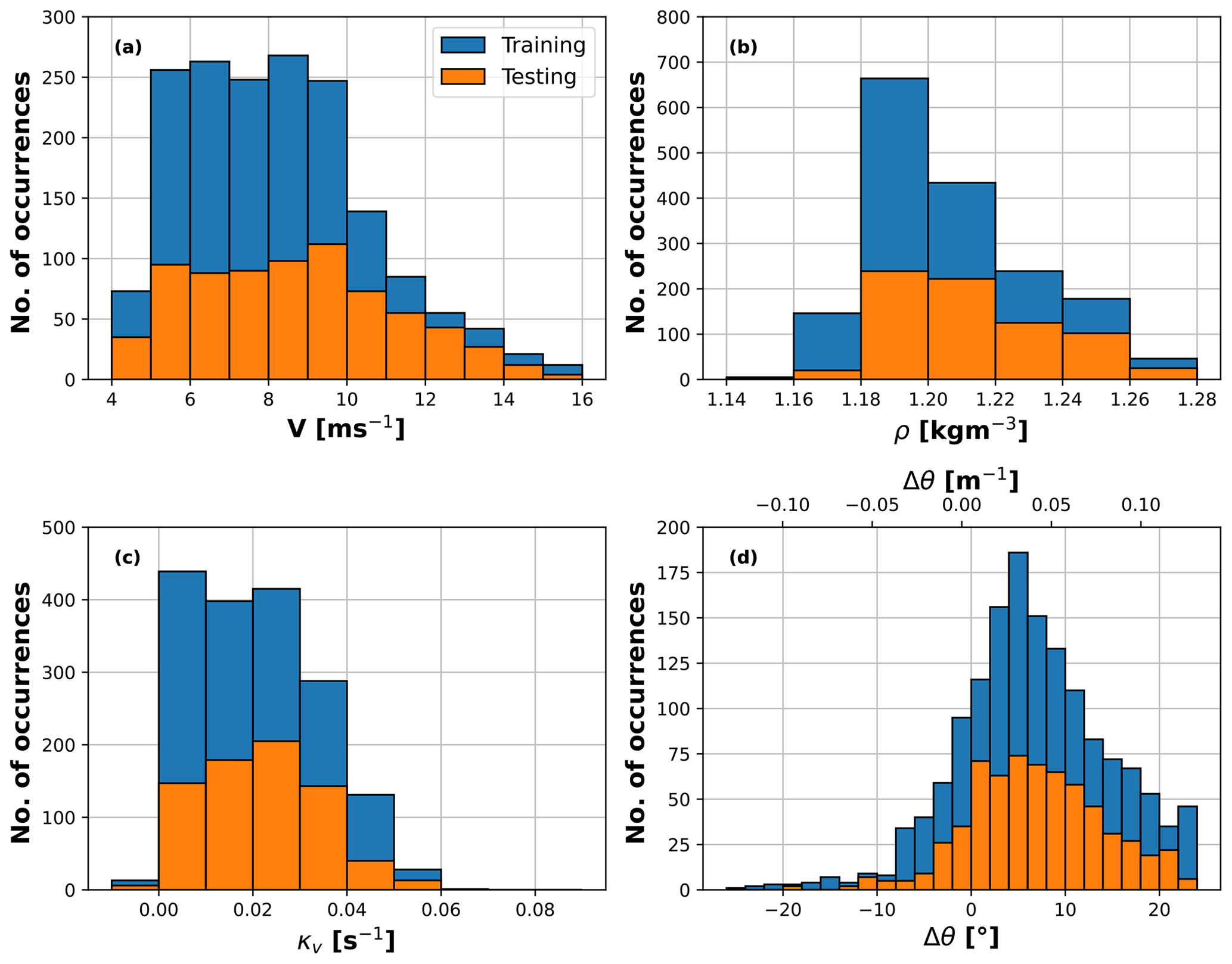
Figure 5 Range and number of occurrences of 10 min averages of wind speed (a), density (b), vertical shear (c), and wind veer (d). Blue – training data set; orange – validation data set.

Air density ρ and wind speed V appearing in the network inputs (see Eq. 4) were measured as follows. Air density was derived from the available measurements of pressure, temperature, and humidity, using the ideal gas laws. Wind speed was obtained by means of an observer based on the standard SCADA signals of power, rotor speed, and blade pitch (Soltani et al., 2013). The use of an observer that is based only on standard operational data renders the shear and veer observers usable on common production machines, where a lidar or a neighboring met mast might not be available. A MoWiT model (Fricke et al., 2021) of the AD8 turbine was used to generate a lookup table (LUT) offline, storing the dependency of produced power on ambient wind speed, pitch angle, and rotor speed, considering mechanical losses in the drivetrain and the efficiency of the generator. Next, the LUT was inverted by a Newton iteration using the aerodynamic torque obtained from the dynamic torque-balance equation, and on measured power, pitch and rotor speed from the SCADA data stream; rotor acceleration was obtained by deriving the measured rotor speed with respect to time. Figure 6 shows the correlation between 10 min averages of the rotor-effective wind speed (REWS) from the observer, reported on the y axis, and the wind speed obtained by averaging the available lidar measurements along the rotor height, reported on the x axis. The match between these two quantities is characterized by a Pearson coefficient of 0.98 and a MAE of about 0.35 ms⁻¹.

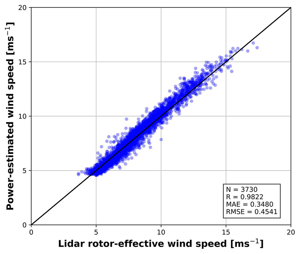
Figure 6 Correlation of 10 min averages between the rotor-average wind speed measured by the lidar (x axis) and the rotor-effective wind speed measured by the observer (y axis). Solid black line – ideal match.

For both the shear and veer observers, the best-performing network configuration was found by trial and error to comprise one single hidden layer and 10 neurons. Both networks took on the order of a few seconds for training on a standard desktop computer.

3.2 Shear and veer observer performance

After training, the two observers of shear and veer were tested on the 10 Hz, 138 h validation data set.

Figure 7 reports the results in terms of 10 min averages. Quantities estimated by the observers are reported on the y axis, while the lidar-measured references are on the x axis. Figure 7a indicates an excellent match for shear, with a Pearson coefficient R=0.947 and an RMSE of about $\mathrm{4.015}\times {\mathrm{10}}^{-\mathrm{3}}$ s⁻¹. Figure 7b indicates a slightly lower quality of the results for veer, with R=0.879 and a larger scatter, as quantified by an RMSE of about 5.78°. MAEs are $\mathrm{3}\times {\mathrm{10}}^{-\mathrm{3}}$ s⁻¹ and 4° for shear and veer, respectively.

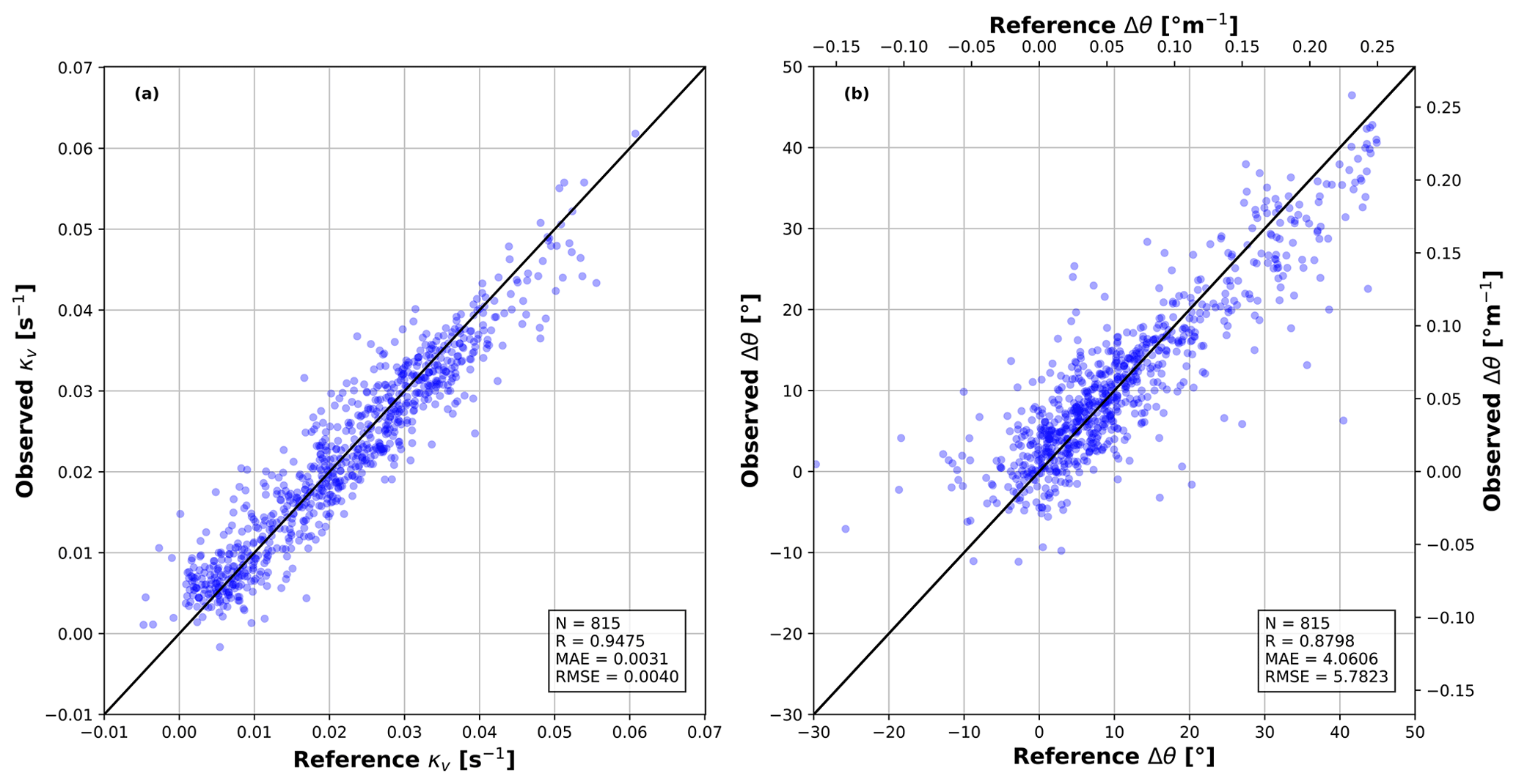
Figure 7 Correlation of 10 min averages between estimated wind characteristics (y axis) and their reference lidar-measured quantities (x axis). Vertical shear κ_v (a); wind veer Δθ (b). Solid black line – ideal match.

Exemplary time histories of observed and reference quantities are given in Fig. 8. Figure 8a and b show the estimated (red) and reference (blue) wind shear and veer, respectively. Additionally, Fig. 8c reports the wind direction at the site, where a horizontal solid black line indicates the 189° direction at which lidar and turbine are aligned. The observation of shear and veer was performed at 1 Hz, and results were then averaged with a 1 min moving window. The figures indicate that the observed quantities follow their respective references quite well, in terms of both trends and mean values. There is a particularly good match between 05:00 AM and 07:00 AM, when lidar and turbine are aligned, although some of the worst matches are between 04:00 AM and 05:00 AM, when the two are also almost aligned. However, the two observers are clearly capable of detecting the diurnal cycle, characterized by higher shear and veer during the night, and also rapid events such as the spike observed around 09:30 AM.

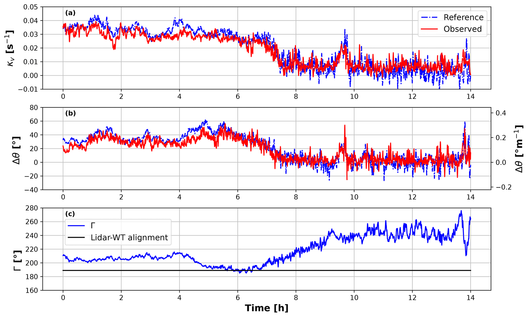
Figure 8 Time histories of vertical shear (a), wind veer (b), and wind direction measured at the mast (c). Blue – observed quantities; red – lidar-measured reference.

Finally, to provide more statistically relevant results, Fig. 9a and b show the MAEs of the observed shear and veer as functions of wind speed for different turbulence intensity (TI) values. Figure 9c reports the number of available data hours for each specific speed and TI bin. MAEs were computed after averaging 1 Hz observations over 10 min and then by comparing them with their respective lidar-measured references. It is difficult to draw strong conclusions as not all wind speed bins are equally populated. In the intermediate wind speed region – where more data points are available – it appears that, as expected, errors are slightly larger for higher TI values. However, in the 7 to 11 ms⁻¹ range, there are more than twice the data points for low (0 %–5 %) TI than for intermediate (5 %–10 %) TI values. It also appears that errors might increase around the lowest and highest wind speeds. This could be due to the smaller loading on the wind turbine in these conditions because of the small dynamic pressure at low wind speeds and because of the large blade pitch at the higher ones. However, these findings should be confirmed by larger and better populated datasets.

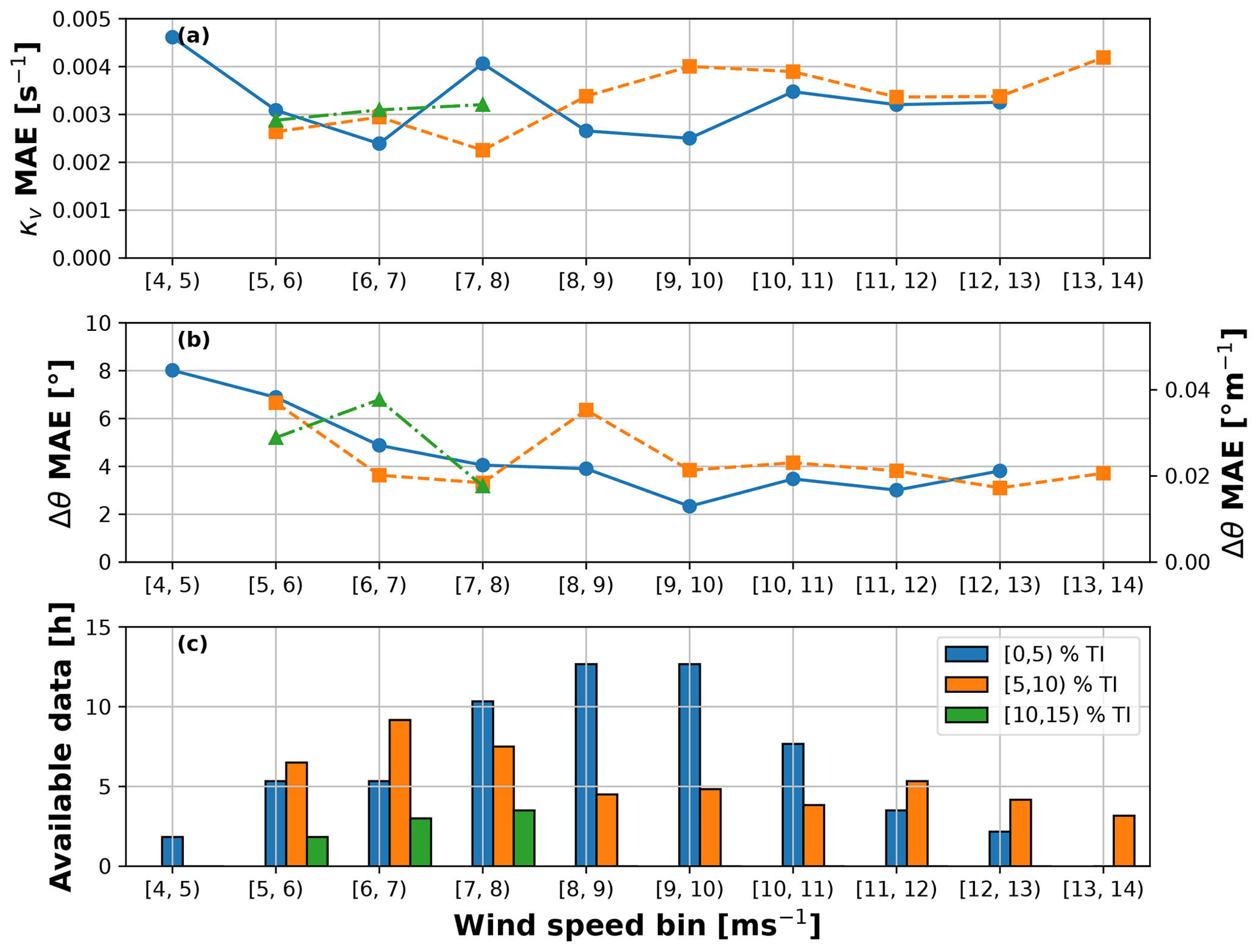
Figure 9 MAE of vertical shear κ_v (a), wind veer Δθ (b), and hours of available data (c) vs. binned rotor-effective wind speed V, for different TI levels.

4 Conclusions

This paper has demonstrated that it is possible to observe vertical wind veer from the operational response of a large wind turbine. The paper also performed the first validation of the observation of shear and veer over the full rotor height with respect to reference measurements obtained using a VP lidar. The study was conducted at the BHV test site using the highly instrumented 8 MW AD8-180 wind turbine. Additionally, the presence of an IEC-compliant met mast on site allowed for a comparison – although limited to only the lower half of the rotor – of the lidar-measured wind speed, shear, and veer, enhancing the confidence in the results.

Based on the results reported herein, the following conclusions can be drawn.

• Correlation between 10 min averages of the observed and lidar-measured shear and veer results in Pearson coefficients of R=0.947 and R=0.879, respectively. The quality of shear is presumably better because its observation relies on only 1P harmonics, whereas veer requires also the 2P components, which are probably more affected by turbulence.

• For the same reason, veer has a higher scatter than shear, as seen in Fig. 7.

• Both the shear and veer observers seem capable of tracking both slow and relatively fast changes in ambient conditions. In particular, the exemplary time history reported in Fig. 8 indicates the ability to follow changes in duration of tens of minutes with good accuracy. The examination of other similar time histories, not reported here for brevity, supports and confirms this finding.

• Definitive conclusions on the effects of TI and speed on the quality of the estimates are not possible because of the uneven population of the bins. However, results aggregated over the whole validation data set indicate typical MAEs of approximately 4° for veer and around $\mathrm{3}\times {\mathrm{10}}^{-\mathrm{3}}$ s⁻¹ for shear.

In general, these results seem to indicate the ability of the harmonic-based observers to estimate shear and veer from the operational response of a wind turbine, with a close match to the widely adopted vertical profiling lidar. In evaluating these results, however, two remarks are in order.

• The lidar measurements cannot be assumed to be an absolute ground truth. In fact, as is the case with all measurements, they are affected by various sources of error, and they represent spatial and temporal averages that differ from the ones performed by the observer and by the anemometry installed on the mast. Additionally, the lidar is not exactly co-located with the turbine; it is not always exactly in front of it, and it does not even span exactly the same height as it starts measuring a small distance above the LBT. Therefore, an exact match between observers and lidars cannot and should not, in general, be expected. One source of discrepancy could be removed by the use of a forward-staring lidar, which would at least always provide wind measurements directly upwind of the turbine.

• Some of the speed and TI bins are not well populated, which might have some effect on the significance of the performance statistics. This source of uncertainty could be removed by the use of longer data sets that, however, were not available for this study.

Appendix A: Harmonic content of the observers

Following Eggleston and Stoddard (1987), an elementary model of blade dynamics can be obtained by considering a rigid flapping blade connected to the rigid hub by a hinge, as shown in Fig. A1.

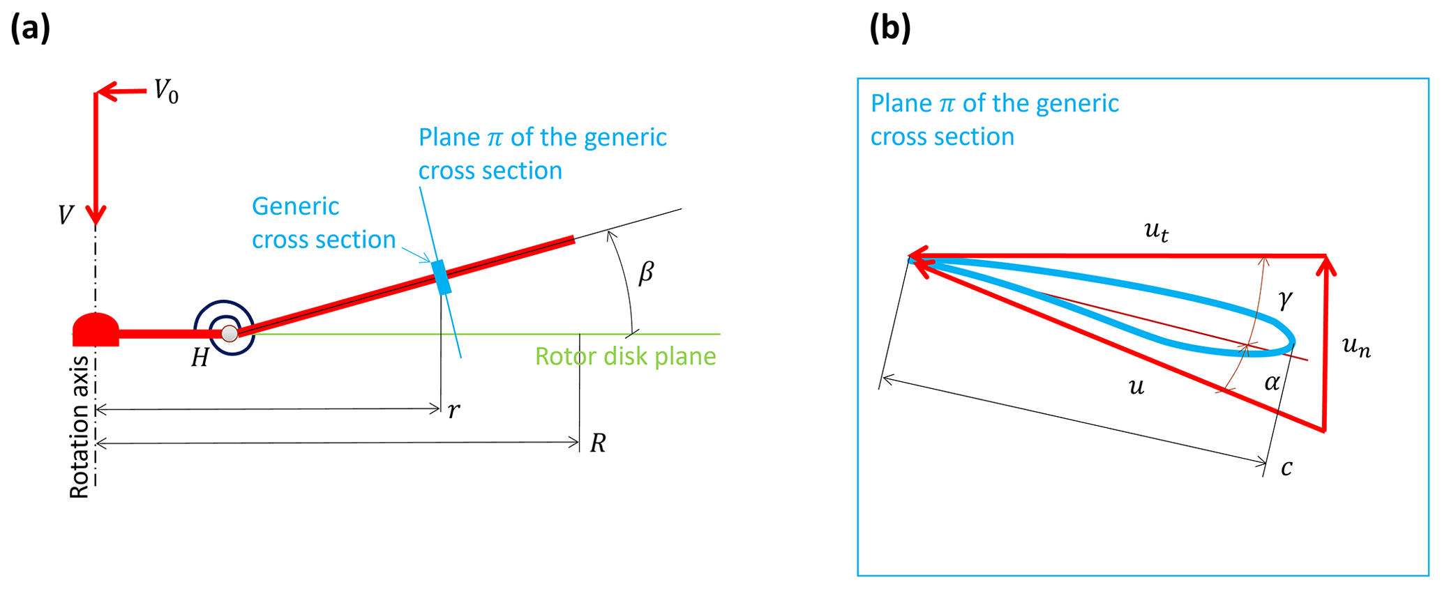
Figure A1 Elementary model of a flapping blade. Panel (a) is the side view, with the rigid flapping segment hinged at the rigid hub at point H. Panel (b) is the view perpendicular to the plane of the cross section showing the section-relative flow components u_n and u_t.

The flow speed components normal (named u_n) and tangential (named u_t) to a generic cross section of the flapping blade can be written as

$$\begin{array}{}\text{(A1a)}& {\displaystyle }{u}_{\mathrm{n}}=V(\mathrm{1}-a)-V{\mathit{\kappa }}_s{\displaystyle \frac{r}{R}}\cos \mathit{\psi }-V_{\mathrm{0}}\mathit{\beta }\sin \mathit{\psi },\text{(A1b)}& {\displaystyle }{u}_{\mathrm{t}}=\mathrm{\Omega }r,\end{array}$$

where a is the axial induction, β is the (small) blade flap angle, ψ is the azimuthal blade position (where ψ=0 when the blade is vertical pointing downwards), r is the spanwise position of the cross section, R is the rotor radius, V₀ is the cross-flow (i.e., a lateral wind speed component parallel to the rotor disk plane), and Ω is the rotor speed. When the inflow presents a veer, Δθ, the cross-flow can be written as $V_{\mathrm{0}}=\mathrm{\Delta }\mathit{\theta }(r/R)\cos \mathit{\psi }$. The flapwise bending moment on the blade is obtained by integrating the lift L along the blade span, to yield

$$\begin{array}{}\text{(A2)}& L={\displaystyle \frac{\mathrm{1}}{\mathrm{2}}}\mathit{\rho }{u}^{\mathrm{2}}c{C}_{{\mathrm{L}}_{\mathit{\alpha }}}\mathit{\alpha }\approx {\displaystyle \frac{\mathrm{1}}{\mathrm{2}}}\mathit{\rho }c{C}_{{\mathrm{L}}_{\mathit{\alpha }}}(u_{\mathrm{n}}{u}_{\mathrm{t}}-\mathit{\gamma }{u}_{\mathrm{t}}^{\mathrm{2}}),\end{array}$$

where u≈u_t is the flow speed at the blade section, c is the chord, $C_{{\mathrm{L}}_{\mathit{\alpha }}}$ is the lift slope, $\mathit{\alpha }\approx u_{\mathrm{n}}/u_{\mathrm{t}}-\mathit{\gamma }$ is the angle of attack (considering small angles), and finally γ is the pitch angle.

Inserting the expressions for u_n and u_t given by Eq. (A1) into Eq. (A2), it follows that lift, and hence bending moments, depends on terms proportional to κ_scos ψ and Δθsin ψcos ψ=2Δθsin (2ψ). Thus, shear leaves a mark on the 1P harmonic of blade loads and veer on their 2P harmonics.