Uncertainty quantification of structural blade parameters for the aeroelastic damping of wind turbines: a code-to-code comparison

Uncertainty quantification (UQ) is a well-established category of methods to estimate the effect of parameter variations on a quantity of interest based on a solid mathematical foundation. In the wind energy field most UQ studies focus on the sensitivity of turbine loads. This article presents a framework, wrapped around a modern Python UQ library, to analyze the impact of uncertain turbine properties on aeroelastic stability. The UQ methodology applies a polynomial chaos expansion surrogate model. A comparison is made between different wind turbine simulation tools on the engineering model level (alaska/Wind, Bladed, HAWC2/HAWCStab2, and Simpack). Two case studies are used to demonstrate the effectiveness of the method to analyze the sensitivity of the aeroelastic damping of an unstable turbine mode to variations of structural blade cross-section parameters. The code-to-code comparison shows good agreement between the simulation tools for the reference model, but also significant differences in the sensitivities.

1 Introduction

The size of wind turbines has been rapidly increasing over the last decades. As a consequence, current wind turbine blades are more slender and flexible than ever before (Veers et al., 2019). This increases the complexity of turbine vibrations and potentially the probability of aeroelastic instabilities, which raises questions regarding what kind of instabilities are more likely to appear, how state-of-the-art simulation tools compare in their capability to predict this kind of behavior, and how these instabilities can be prevented. Volk et al. (2020) and Kallesøe and Kragh (2016) showed in an experimental validation on a 7 MW, 154 m diameter turbine that instabilities dominated by first and second edgewise modes arise when a modern wind turbine is operated in overspeed.

The required multidisciplinary models to numerically represent these phenomena are complex and have a significant computational cost. Conventional models used in the industry and research employ a multi-body description with beam models for the flexible bodies and blade element momentum (BEM) models, with semi-empirical unsteady extensions, for the aerodynamics. The linear stability behavior is commonly investigated by a linearization of the governing equations around a steady-state equilibrium of the nonlinear system. These models and solution routines depend on numerous parameters, which complicates the identification of the key factors that influence the observed stability behavior. Global uncertainty quantification (UQ) can help identify these crucial factors.

Uncertainty quantification has been a relevant topic in almost all scientific fields. In engineering, it is commonly used to understand physical systems, to improve the design robustness, as a preprocessing step towards model updating and model calibration, or as a component of optimization procedures (Sankararaman, 2012). A comprehensive overview of methods for global sensitivity analysis is given by Iooss and Lemaître (2015). The focus in this paper is on variance-based methods which give a detailed, nonlinear description of the uncertainty in a system, including interactions between parameters. A promising approach to allow detailed global sensitivity analysis on computationally expensive simulations is the introduction of a surrogate model to approximate the full system. Polynomial chaos expansion (PCE) models are becoming increasingly popular for this purpose (e.g., Sudret, 2008; Le Gratiet et al., 2017; Abbiati et al., 2021; Eldred and Burkardt, 2009). They span the full uncertainty domain with a set of orthogonal polynomials. The coefficients of the polynomials are determined by a regression based on samples of the true model. The suitability of surrogate modeling for the analysis of uncertainty propagation in mechanical systems has been shown extensively, e.g., by Hosder et al. (2012) and Scarth et al. (2014) for aeroelastic stability analysis and Nobari et al. (2015) for squeal instabilities; nevertheless, the instability mechanisms for wind turbines can be very different from those on other mechanical systems, so the uncertainties are also likely to be different. A literature overview of UQ studies in the wind energy field is given by van den Bos and Sanderse (2017). Most research efforts have the wind turbine design loads as the quantity of interest (e.g., Roberson et al., 2019; Ziegler and Muskulus, 2016; Gonzaga et al., 2022). Multiple authors successfully applied a surrogate-model-based UQ approach to handle the significant computational cost of the load computations (e.g., Bortolotti et al., 2019; Kumar et al., 2020; Caboni et al., 2020; Hübler et al., 2017, 2019). Comparatively few studies have been performed on uncertainties in wind turbine stability analysis. Resor and Paquette (2011), Lobitz (2005), and Pourazarm et al. (2015b, a) evaluated the impact of uncertainties in the structural and aerodynamic modeling on the flutter speed of an isolated blade by a manual and independent variation of the uncertainty sources. Li and Caracoglia (2019) compared different setups of a polynomial-based surrogate model for the UQ of two interacting uncertain parameters on the flutter speed of an isolated blade. Literature on the uncertainty quantification of full wind turbine stability phenomena is not known to the authors.

To fill this gap, the present article describes a comprehensive methodology for the uncertainty quantification of wind turbine stability analysis. The effect of uncertain beam properties in the elastic blade model on an edgewise whirl wind turbine instability is analyzed. Multiple aeroelastic simulation tools are used in a code-to-code comparison to investigate the influence of the simulation tools on the uncertainty prediction.

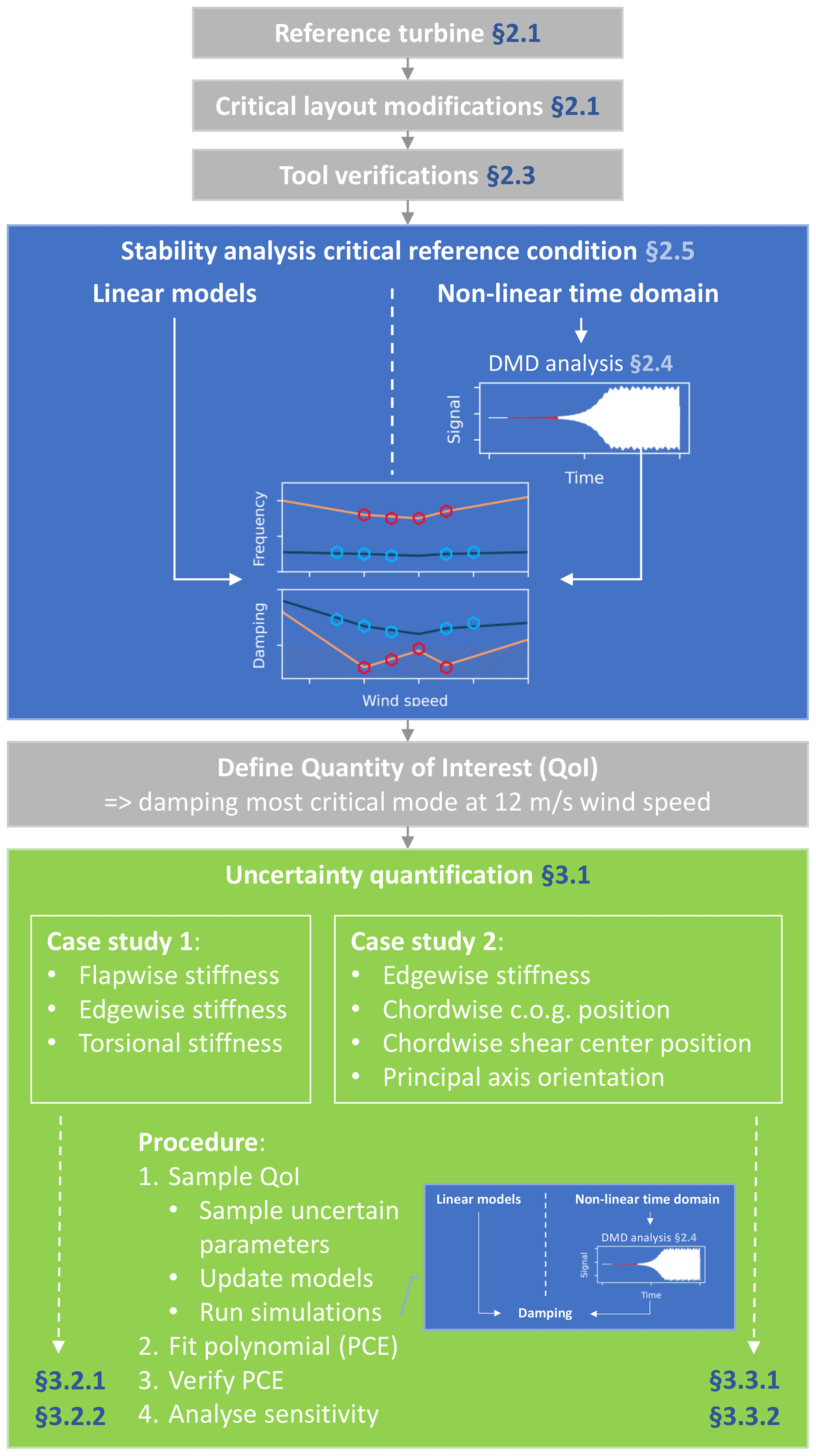
The procedure for this study and the corresponding structure of this article are visualized in Fig. 1. In the default configuration, the IWT-7.5-164 reference wind turbine (Popko et al., 2018) as used in this project shows no aeroelastic instability in the normal operational range. An instability, however, is needed for quantifying the uncertainties. Thus, a change in the blade stiffness was applied such that an edgewise whirl instability formed, similar to those experimentally shown by Volk et al. (2020). This is discussed in Sect. 2.1. This reference condition is simulated with the state-of-the-art simulation tools alaska/Wind, Bladed, HAWC2/HAWCStab2, and Simpack. An OpenFAST model of the reference turbine was established and used for the verification of the other models. However, a stability assessment has not been made with this model because the enforcement of the aeroelastic instability was not successful in this case. The simulation tools are briefly introduced in Sect. 2.2 and their setup is verified in Sect. 2.3. The critical reference condition for the presented tools is compared in detail in Sect. 2.5. On this basis, uncertainty quantification is done with respect to the influence of beam properties on the instability. The damping of the most critical mode will be used as a quantity of interest for the uncertainty quantification. Two academic case studies are performed to show the capabilities of this methodology and to show the comparability and differences in the results between the simulation tools. This is shown in Sect. 3.

Figure 1 Paper overview.

2 Critical reference condition

This section will first describe the wind turbine reference model and the required model modifications to create an interesting instability phenomenon. The wind turbine simulation tools are introduced and the main verification results with this new model are presented. Finally, the critical unstable reference condition is analyzed in detail.

2.1 Reference model

The IWT-7.5-164 open-source reference turbine is used as the baseline configuration (Popko et al., 2018). This turbine was designed according to the environmental conditions defined for wind turbine class IA (IEC, 2005). A detailed code-to-code comparison of this turbine with a focus on the stability behavior with the proposed tools has been presented in Hach et al. (2020). The baseline model has been modified in a couple of respects. The current work focuses on instabilities. Therefore, all asymmetries are excluded from the model to eliminate periodic excitation and resonance effects. This means no gravitational loads, no rotor tilt or yaw, a uniform wind profile, and no tower influence on the wind field. In the nonlinear time domain simulation tools, the tower deflection causes a tilting effect on the rotor plane and the corresponding asymmetry. This effect is difficult to eliminate but causes only a negligible periodic excitation.

Different techniques can be used to introduce an instability for this baseline reference turbine. As presented by Pirrung et al. (2014), the turbine can be operated in a runaway setting. In this kind of simulation, the wind speed increases gradually, and without counteracting generator torque the rotor will accelerate until an instability arises. This procedure has the disadvantage that the operating condition at the instability varies between tools, as shown for the IWT turbine in Hach et al. (2020). This introduces an additional uncertainty and might complicate the comparison between said tools. Additionally, the runaway critical operating condition might be far above nominal rotor speeds, reducing the comparability with realistic operational conditions. Instead, the physical properties of the turbine are manipulated in order to enforce an instability under nominal operating conditions. A priori, the sensitivity of the turbine stability to the model parameters was unknown. The model manipulation was therefore a trial-and-error process based on engineering knowledge. Only the flapwise, edgewise, and torsional stiffness of the blades were modified with a uniform scaling factor along the blade to keep the parameter space limited. The stiffness reductions were done on the 6×6 stiffness matrices, which were computed with BECAS (Blasques et al., 2016), and served as a reference for all other tools. The resulting aeroelastic behavior for different sets of scaling factors was analyzed iteratively in HAWCStab2. A stiffness reduction of 70 % in the flapwise direction, 30 % in the edgewise direction, and 70 % in the torsional direction was required to accomplish the desired instability behavior.

2.2 Wind turbine simulation tools

In this research, a comparison is made between multiple state-of-the-art aeroelastic simulation tools. All tools are based on the same category of low-fidelity engineering models. The main model properties are summarized in Table 1. For a detailed understanding of the respective models, readers are referred to the scientific literature and manuals describing the theory and capabilities of the models which are included in the table. The table and the discussion in this section only highlight the most important differences.

IfM (2018)Schubert et al. (2017)DNV (2023)Collier et al. (2015)Larsen and Hansen (2021)Kim et al. (2013)Gözcü and Verelst (2020)Hansen et al. (2004)Sørensen and Aagaard Madsen (2006)NREL (2023)Wang et al. (2017)Jonkman et al. (2017)Dassault Systemes (2021)Wallrapp (2017)Moriarty and Craig Hansen (2005)DNV (2023)Collier et al. (2015)Hansen et al. (2018)Hansen (2004)Hansen (2011)Hansen et al. (2004)Sørensen and Aagaard Madsen (2006)

Table 1 Overview of the features of the simulation tools used.

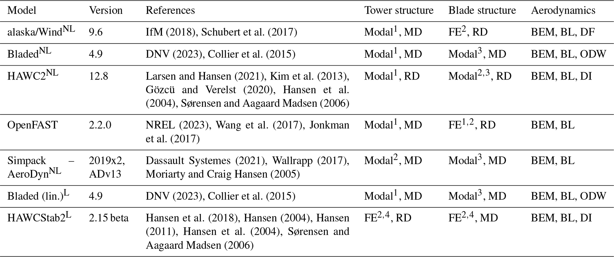
^NL Nonlinear time domain simulation tool, ^L linear model, FE: finite element, MD: modal damping, RD: Rayleigh damping, ¹ single-body, internal finite-element analysis (FEA), ² internal model based on 6×6 mass and stiffness matrices, ³ multipart modal reduction, internal FEA, ⁴ nonlinear co-rotational kinematics, BEM: blade element momentum theory, BL: Beddoes–Leishman dynamic stall model, DF: dynamic flex wake model, ODW: Øye dynamic wake model, DI: dynamic inflow model.

Two categories of simulation tools can be distinguished. Bladed (lin.) and HAWCStab2 provide linear models (at nonlinear equilibrium points), which will be used for standard linear stability analysis. On the other hand, alaska/Wind, Bladed, HAWC2, OpenFAST¹, and Simpack–AeroDyn will be used in this work for nonlinear time domain simulations. The post-processing methodology to analyze the stability properties of these simulations will be discussed in Sect. 2.4. Preliminary comparisons have indicated that it is crucial to capture both the geometric coupling effects and nonlinear deformations of the blades, in addition to accounting for unsteady aerodynamic effects. Some differences exist in the corresponding theories underlying the implementations in the different tools. The structural blade models in alaska/Wind, HAWC2, HAWCStab2, and OpenFAST use the reference 6×6 mass and stiffness matrices directly for an exact model of the geometric coupling effects (Schubert et al., 2017; Kim et al., 2013; Hansen, 2011; Wang et al., 2017). Bladed and Simpack use beam properties derived from the 6×6 matrices which include coupling effects due to offsets between the shear and elastic centers (DNV, 2023; Wallrapp, 2017). Geometrically nonlinear effects are incorporated through a multi-body segmentation in Bladed, HAWC2, and Simpack, while alaska/Wind, OpenFAST, and HAWCStab2 use a direct internal nonlinear finite-element analysis (Collier et al., 2015; Gözcü and Verelst, 2020; Schubert et al., 2017; Wang et al., 2017). All tools use a Beddoes–Leishman-like dynamic stall model. Alaska/Wind, Bladed, HAWC2, and HAWCStab2 additionally include a dynamic wake model, which was not available for the OpenFAST and Simpack models (DNV, 2023; Hansen et al., 2004; Sørensen and Aagaard Madsen, 2006; Jonkman et al., 2017; Moriarty and Craig Hansen, 2005). The final noteworthy difference among the tools lies in their control systems. The primary aim was to mitigate control system impact on the stability results through open-loop control configurations with fixed operating conditions. This was not possible in all tools. In the alaska/Wind and Bladed time domain simulations special controllers were used, which were tuned to keep the rotational speed as constant as possible. The resulting variations in rotational speed were negligible.

2.3 Model verification

The simulation tools used in this work were previously compared for the same reference turbine but without the stiffness reductions by Hach et al. (2020). A similar strategy with test cases of increasing complexity was also applied for this new reduced stiffness reference model. The most notable results are discussed here.

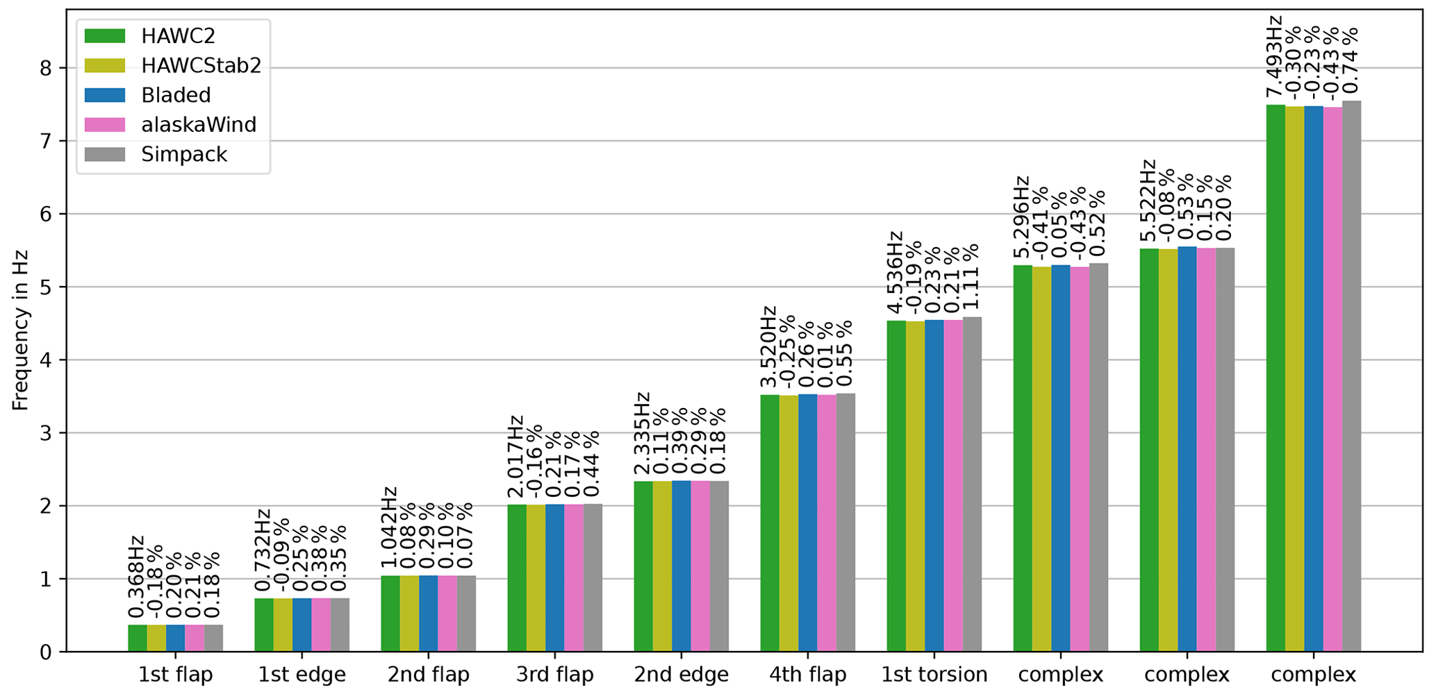
The isolated, clamped blade eigenfrequencies are shown in Fig. 2. All tools are in excellent agreement. The relative difference between the tools is less than 0.5 % for the first five modes. The deviations increase for higher-frequency modes but remain below, or close to, 1 %. The Simpack eigenfrequencies show the largest deviation, especially for modes with a high torsional content.

Figure 2 Comparison of isolated blade eigenfrequencies.

As a second comparison, a steady quintuple gravitational load is imposed on the clamped blades. The blades are positioned both with the suction side downwards, such that gravitational loading is in the flapwise direction, and with the leading edge downwards such that the gravitational loading is in the edgewise direction. The gravitational loading multiple is representative for nominal operational loads. The results for the flapwise loading are shown in the left column of Fig. 3 and for the edgewise loading in the right column. The translational deflections in the direction of the loading are in excellent agreement. Small deviations arise for the deflections in the direction perpendicular to the loading, especially for the flapwise deflection under edgewise loading. The main point of difference is the representation of the torsional component. Significant differences exist between all tools with discrepancies up to 0.5°. The unphysical oscillations towards the tip in the OpenFAST result were also observed in Hach et al. (2020) and are likely due to a faulty blade curvature and twist calculation with the internal cubic spline fit in BeamDyn (NREL, 2019).

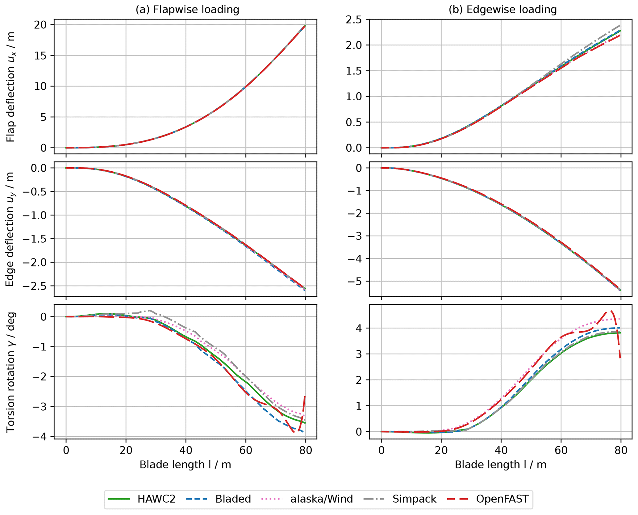
Figure 3 Comparison of isolated blade deflections under steady quintuple gravitational loads.

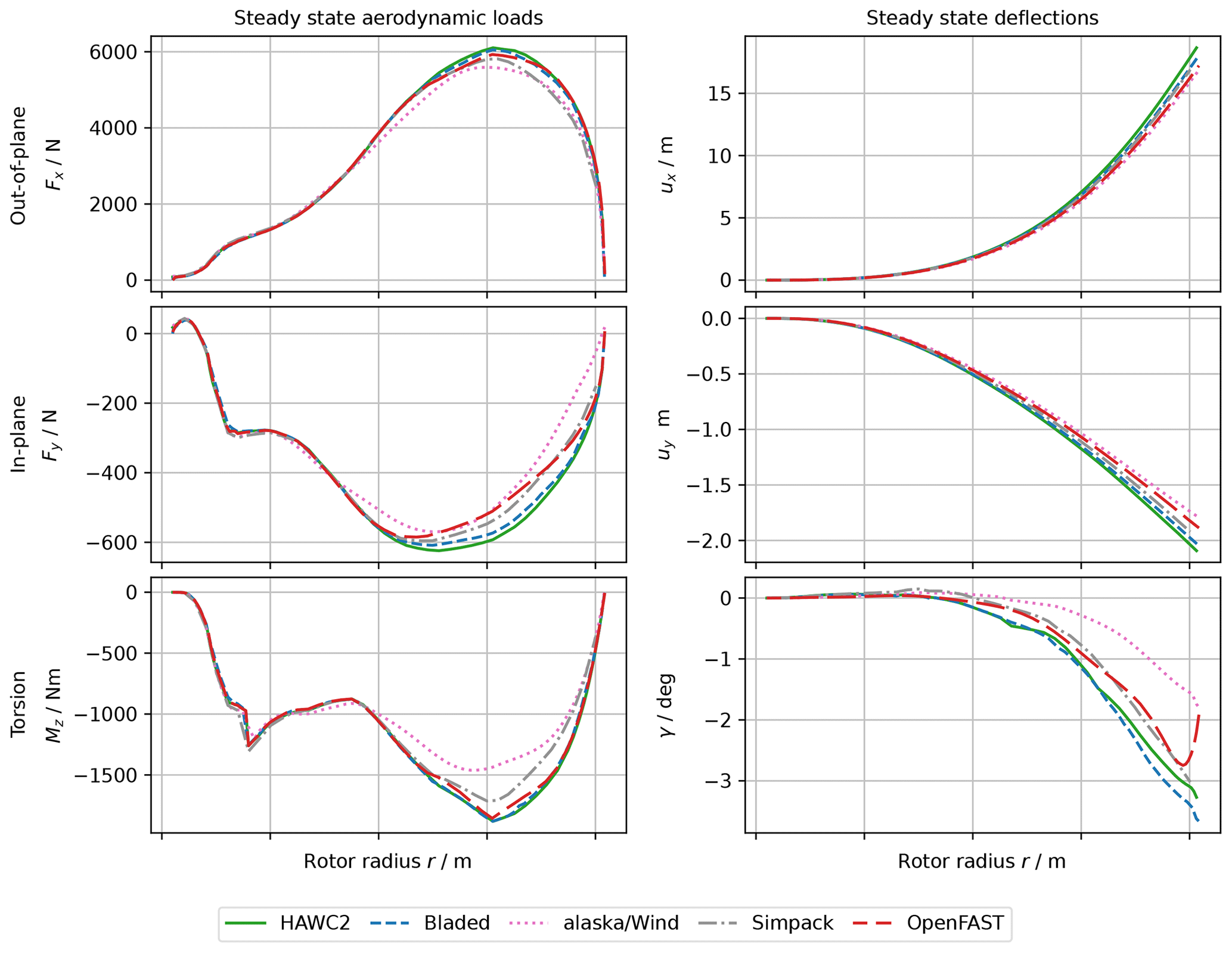
The final verification test shows the static aeroelastic equilibrium for a rotor system with rigid tower in a uniform, steady wind field with a velocity of 10 m s⁻¹. The rotor blades in this test are the only flexible component of the turbine. The steady-state aerodynamic loads are shown in the left column of Fig. 4, and the corresponding steady-state deflections are shown on the right-hand side. Due to the increased complexity, the agreement between the tools deteriorated in comparison with the static deformation case above. Nevertheless, the overall agreement is reasonable. Alaska/Wind shows the largest discrepancy with respect to the other tools, with lower loads in all directions and therefore also consistently lower deformations. The OpenFAST result also shows the unphysical oscillation in the torsional deformation near the tip of the blade.

Figure 4 Comparison of the aeroelastic steady-state loads and deflections of the full rotor.

2.4 Damping determination from time domain simulations

To allow a stability assessment based on the time domain simulations, the damping of the system has to be determined from the resulting time signals. Multiple approaches can be used to achieve this. Riziotis and Voutsinas (2006) used two different methods: the first method was based on the gradient of peaks in the amplitude spectrum of a moving FFT window, and the second method was applied directly to the signal amplitude envelope by means of a Hilbert transform. Volk et al. (2020) used logarithmic decrement analysis on a signal after a bandpass filter was applied around a predefined frequency. Wanke et al. (2020) used an exponential fitting on the oscillatory signal after excitation on the three blades at the desired frequency and desired phase difference between the blades.

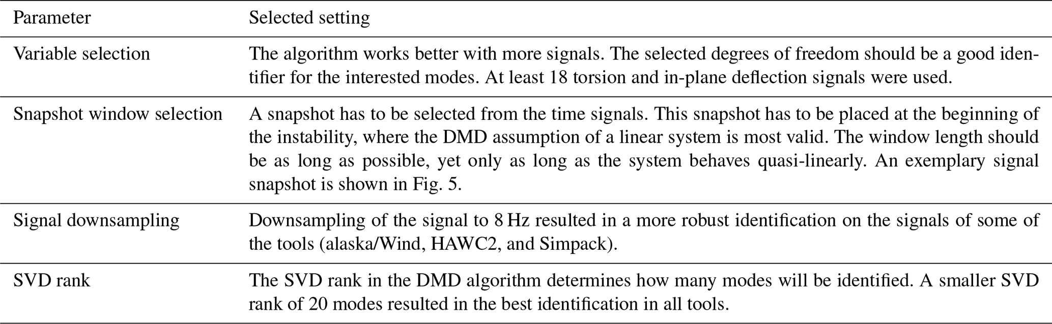
In this work, a different approach based on the dynamic mode decomposition (DMD) method is used. The higher-order DMD formulation by Le Clainche and Vega (2017) was applied, which is available in the open-source Python package pyDMD. For a detailed theoretical description of the method, please refer to Le Clainche and Vega (2017). This method describes the signal in a spatiotemporal manner; i.e., it can be used to decompose a signal in spatial modes with corresponding frequency and damping content. For linear aeroelastic systems, this would mean that the exact physical modes can be extracted. For nonlinear systems, DMD can be understood as a best-fit linear operator on the nonlinear signal. This method is fully data-driven, which is an important characteristic if the methodology has to be applied to simulation tools with restricted access to the source code. The only required inputs are snapshots of the time signals. Note that these signals were transformed into the inertial reference system with a multiblade coordinate transformation (MBC) (Bir, 2008). The accuracy and robustness of DMD can depend strongly on the selection of these snapshots and the configuration parameters of the DMD method. The configurable parameters and their selected settings are shown in Table 2. It is worth mentioning that a fully automated post-processing has not been achieved. Some of the parameters in Table 2 cannot be applied equally for all the results. A full list of the choices is beyond the scope of this article, but it is part of the data package published in Verdonck et al. (2023a).

Table 2 DMD damping determination settings.

For completeness, it is important to mention that a number of other methods to determine the damping from time signals were attempted without success. Computing the logarithmic decrement from subsequent oscillation peaks, exponential curve fitting on the oscillation peaks, and linear curve fitting on logarithmic data all share the assumption that the signal only has a single degree of freedom. Their accuracy is largely dependent on a smooth, linear signal, and they therefore did not produce robust results for the multi-degree of freedom, nonlinear results of the wind turbine simulation tools. Attempts with bandpass filtering of the signal for a specific frequency range did not lead to robustness improvements.

2.5 Comparison between Campbell plots and time domain runs

The final stability analysis of the reference condition is shown as a Campbell diagram in Fig. 6. This reference condition was presented earlier in Verdonck et al. (2021) but will be discussed here in more detail. Figure 6a shows the HAWCStab2 and Bladed (lin.)² linearization results. Only the properties of the first and second edgewise whirling modes are shown. These are the only modes of the system which become unstable. One can see an almost exact match in the frequency progression between the tools. The trend of the damping curves is also in agreement. The first edgewise backward whirling (BW) and forward whirling (FW) modes have a double-dip trend with the most negative damping values around 10 and 13 m s⁻¹. The second edgewise BW and FW modes show a steady decrease in damping until 12 m s⁻¹, followed by a consistent increase. The absolute damping values show some differences. The HAWCStab2 damping is lower for the first edgewise BW mode and the second edgewise modes. The opposite is true for the first edgewise FW mode. The absolute differences for the second edgewise modes are significantly smaller than the differences for the first edgewise modes.

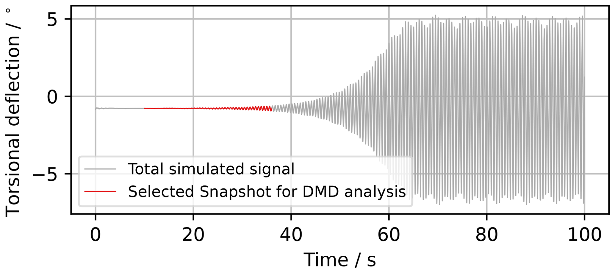
Figure 5 Exemplary snapshot selection for the DMD analysis. This exemplary signal is the torsional deformation of one of the blades at 50 m blade length.

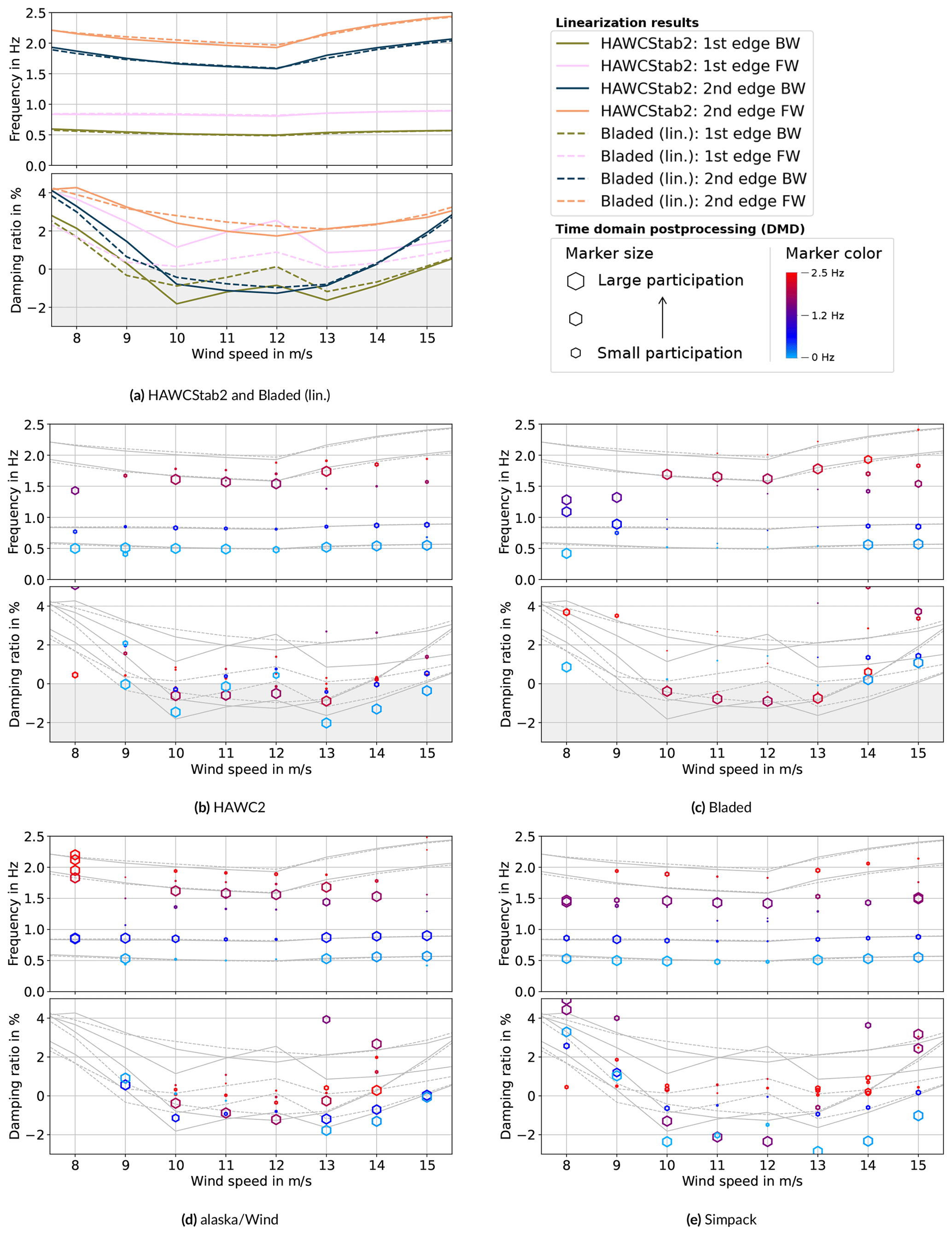
Figure 6 Linearizations (colored lines in a, gray lines in b–e) and time domain simulations post-processed with DMD (markers in b–e).

Figure 6b–e show the comparison with each of the time domain tools. Time domain simulations were executed at each of the eight wind speeds (8, 9, …, 15 m s⁻¹). As described in Sect. 2.4, the MBC-transformed time signals were post-processed with DMD to obtain the modal content in the signal. These results are shown by the colorful hexagonal markers in both the frequency and damping plots. The size of these markers indicates their participation in the signal. This is particularly useful to identify modes which have significant participation in unstable signals. The color scale of the markers indicates the frequency of the mode to be able to link the DMD markers between the damping and frequency plot. The HAWCStab2 and Bladed (lin.) linearization results are repeated in each of these plots by the gray lines in the background. First, the overall results of the DMD post-processing of the time domain tools in comparison to the linearizations will be discussed, followed by a discussion of the most noticeable deviations or details of the individual tools.

Overall, clear correlations between the DMD post-processed time series and the linearizations can be found. The time domain simulations of almost all tools are unstable in the same wind speed range from 10 m s⁻¹ up to 15 m s⁻¹. For most tools, the first and second edgewise modes are identified accurately for the unstable time simulations. Moreover, a similar trend over the wind speeds appears. The first edgewise BW mode has the lowest damping at low and high wind speeds (9–10 and 13–15 m s⁻¹) but a slightly higher and sometimes positive damping around rated wind speeds (11–12 m s⁻¹). On the other hand, the damping of the second edgewise BW mode monotonously decreases up to 12 m s⁻¹ and increases afterwards. This results for almost all tools in an instability mechanism dominated by the first edgewise BW mode at lower wind speeds (<11 m s⁻¹), dominated by the second edgewise modes at middle wind speeds (11–12 m s⁻¹), and dominated again by the first edgewise mode at higher wind speeds (>12 m s⁻¹). The DMD setup in this project is tuned to identify the unstable or marginally stable modes. The application of the same method to stable or highly damped time series was out of the scope. This makes the applied methodology not suitable for stable operating points (e.g., 8 m s⁻¹), where poor agreement between the DMD processed time series and the linearizations can be found. In order to generate a full Campbell diagram, the DMD identification of all modes, regardless of their damping, could be the subject of further studies.

A closer look at the DMD results of the individual tools shows the following peculiarities. The HAWC2 time domain results agree on the whole well with the HAWCStab2 linearization. Two small differences are the overall slightly lower frequency of the second edgewise BW mode and the higher damping of this same mode at 11 and 12 m s⁻¹. The Bladed time domain simulations are only unstable for the operating points between 10 and 13 m s⁻¹. The identified second edgewise BW mode is an excellent match in both frequency and damping to the Bladed linearization. The first edgewise BW modal component is also identified, but its participation in the time signal is significantly smaller and the damping ratio is higher compared to the linearization results and the other time domain simulations. This explains why the time simulations with Bladed are stable at 14 and 15 m s⁻¹, where the other tools experience the first edgewise BW-dominated instability mechanisms. The reason for this difference between the Bladed time domain result and the other tools, especially with respect to the Bladed linearization, is unknown. The DMD post-processing is unlikely to be the cause of the difference, as it accurately identifies the second edge BW mode and as it correctly identifies exclusively positively damped modes for the stable simulations at 9 and 14 m s⁻¹. In alaska/Wind, the first edgewise FW mode has a significantly lower damping compared to all other tools. At 10 m s⁻¹ this even becomes the lowest damped mode. The frequency of the second edgewise BW mode is also slightly below the linearization results. Besides this, the trend and magnitude of both the frequencies and damping of the first and second edgewise BW modes agree well with the linearizations. The Simpack results show some significant differences with respect to the linearizations and the other tools. The second edgewise modes have a significantly lower frequency. Furthermore, although the trend correlates well with the linearizations, the magnitude of the damping of the first and second edgewise modes is significantly lower. The root cause of this difference is unknown.

3 Uncertainty quantification case studies

Two case studies were performed on the influence of structural beam properties on the critical reference condition. Case study 1 is a basic study with a limited number of easily understandable uncertain parameters which serves as a demonstration and verification of the overall process. Case study 2 is a step closer towards engineering practice and serves as a mock-up case study for the analysis of the influence of blade manufacturing defects on the aeroelastic stability.

The case studies are limited to the operating point at 12 m s⁻¹ wind speed of the critical reference condition presented in Sect. 2. This can be interpreted as a single vertical slice of the Campbell diagrams in Fig. 6. The operating conditions (wind speed, rotor speed, pitch) are kept constant for all model variations during the uncertainty quantification. This results in varying torque and power production. This was done to increase the reproducibility and simplify the comparison between the different tools such that differences in the stability analysis and differences in the sensitivity of the uncertain parameters to the stability are most likely the result of differences in the structural dynamic and aerodynamic modeling in the tools. The damping ratio of the most critical mode was selected as the quantity of interest (QoI) for the uncertainty quantification; i.e., the influence of the uncertain parameters on the damping of this mode will be analyzed. The mode with the lowest damping at 12 m s⁻¹ is for all tools the second edgewise BW mode with a frequency of approximately 1.55 Hz and damping ratios varying between −2.35 % and −0.5 %.

3.1 Uncertainty quantification (UQ) framework

A non-intrusive, global, variance-based uncertainty quantification based on a PCE surrogate model will be used in this work. This methodology does not require a modification of the simulation codes and by means of the surrogate model, the required number of simulations can be reduced significantly compared to a standard Monte Carlo simulation. The uncertainty quantification covers the full domain spanned by the uncertain parameter distributions and captures the potential interaction between these parameters.

The Python implementation of the preprocessor, post-processor, and interfaces to the tools is available open-source in the framework wtuq (Verdonck et al., 2023b, 2022). This framework uses the open-source packages uncertainpy and chaospy for the setup of the PCE model and uncertainty evaluation (Tennøe et al., 2018).

3.1.1 Surrogate model

Polynomial chaos expansion (PCE) with point collocation is used as a surrogate model. The applied PCE models had a fourth-order polynomial. The quasi-random Hammersley sampling scheme was used and the number of training data points for a given number of uncertain parameters were based on the best-practice findings by Hosder et al. (2007). The accuracy of this setup was tested by decreasing and increasing the polynomial order and increasing the number of sampling points for some tools. This did not lead to significant improvements or deteriorations in the accuracy of the PCE model.

Verification of the PCE model is necessary to ascertain that the surrogate is a good representation of the true model. As an initial verification measure, the surrogate model can be evaluated at the training data coordinates. However, this measure can be influenced by overfitting. Therefore, a leave-one-out test should be used as cross-validation. This test is done by the computation of an individual leave-one-out surrogate model for each of the training data points. This surrogate model does not contain that specific training data point. A comparison of this leave-one-out surrogate model evaluated at the coordinates of the training data point and the true model evaluation at those coordinates is then done. In general, the computation of the surrogate model is not expensive, but as shown by Le Gratiet et al. (2017), an exact mathematical computation of the leave-one-out error without recomputation of the surrogate model for each of the training data points is also possible.

Alternatively, additional random control points, which are not contained in the training dataset, could be used for verification. The leave-one-out error has the benefit over adding random control point computations that no additional simulations are required. The downside is that the leave-one-out error might introduce additional errors, especially at the edges of the input parameter space, because it assembles new surrogate models, missing the data point where the leave-one-out error is computed.

Based on the training data and the leave-one-out surrogate model, two error estimation metrics are defined, which are as follows.

$$\begin{array}{}\text{(1)}& {\displaystyle }\begin{array}{rl}& \text{Normalized root mean square deviation:}\\ & \text{NRMSD}={\displaystyle \frac{\sqrt{\frac{\sum {\left(\widehat{X}-X^{*}\right)}^{\mathrm{2}}}{n}}}{max\left(X^{*}\right)-min\left(X^{*}\right)}}.\end{array}\text{(2)}& {\displaystyle }\begin{array}{rl}& \text{Mean absolute error:}\\ & \text{MAE}={\displaystyle \frac{\sum \left|\widehat{X}-X^{*}\right|}{n}}.\end{array}\end{array}$$

Here, X^* is the set of training data samples of the quantity of interest, $\widehat{X}$ is the set of approximated quantities of interest of the leave-one-out surrogate model, and n is the number of samples.

3.1.2 Uncertainty quantification

The uncertainty quantification is done on the PCE surrogate model. It is common to use the Sobol indices as global uncertainty quantification metrics. They are a measure for the contribution of each uncertain input parameter to the variance of the output quantity of interest. Two Sobol indices will be used in this paper. The first-order Sobol index is given by

$$\begin{array}{}\text{(3)}& S_i={\displaystyle \frac{\mathbb{V}\left[\mathbb{E}\left[X|Q_i\right]\right]}{\mathbb{V}\left[X\right]}}\end{array}$$

and represents the isolated contribution of an uncertain parameter to the total output variance. 𝕍[𝔼[X|Q_i]] is the variance of the expected value of the quantity of interest X, given only the uncertainty distribution of the uncertain parameter Q_i. 𝕍[X] is the total variance of the quantity of interest, including all uncertain parameters. The total Sobol index is given by

$$\begin{array}{}\text{(4)}& S_{Ti}=\mathrm{1}-{\displaystyle \frac{\mathbb{V}\left[\mathbb{E}\left[X|Q_{-i}\right]\right]}{\mathbb{V}\left[X\right]}}\end{array}$$

and represents the contribution of an uncertain parameter to the total output variance, including interactions with other parameters. $\mathbb{V}\left[\mathbb{E}\left[X|Q_{-i}\right]\right]$ is the variance of the quantity of interest given the contributions of all uncertain parameters, except the contribution of parameter Q_i. As shown by Sudret (2008), the Sobol indices of a PCE model can be computed analytically exclusively on the basis of the coefficients of the polynomial.

The Sobol indices condense the uncertainty into single values. This is a clear metric for both the contribution of a parameter to the total variance in a model and the interaction between parameters, but it does not give insight into the way an uncertain parameter influences the quantity of interest. This detailed view can be given at a negligible computational cost by analyzing the polynomials of the PCE model along the different uncertain dimensions.

3.2 Case study 1: verification

This case study applies three straightforward uncertain parameters: flapwise, edgewise, and torsional stiffness of the blades. These uncertain parameters are given identical uncertainty distributions. The radial discretization of the uncertainties is determined by a nonuniform rational B-spline (NURBS), similar to the methodology proposed by Kumar et al. (2020). In this case, the spline is fixed at the root and tip of the blade and a single control point in the center determines the shape of the NURBS curve. This methodology has been shown in Verdonck et al. (2022). The uncertain parameters are uniformly distributed and resulted in a maximum modification of the nominal stiffness values in the center of the blade of approximately ±5 %.

Note that to guarantee a correct modification of the parameters in the different tools, said modifications are done directly on the reference 6×6 mass and stiffness matrices (Hodges, 2006). The implementation can be found in the Python modules in the software repository (Verdonck et al., 2023b). Each variation has been verified by a comparison of the structural blade eigenvalues in the different tools for the individual parameter modifications. The same procedure was used for the parameter modifications of case study 2.

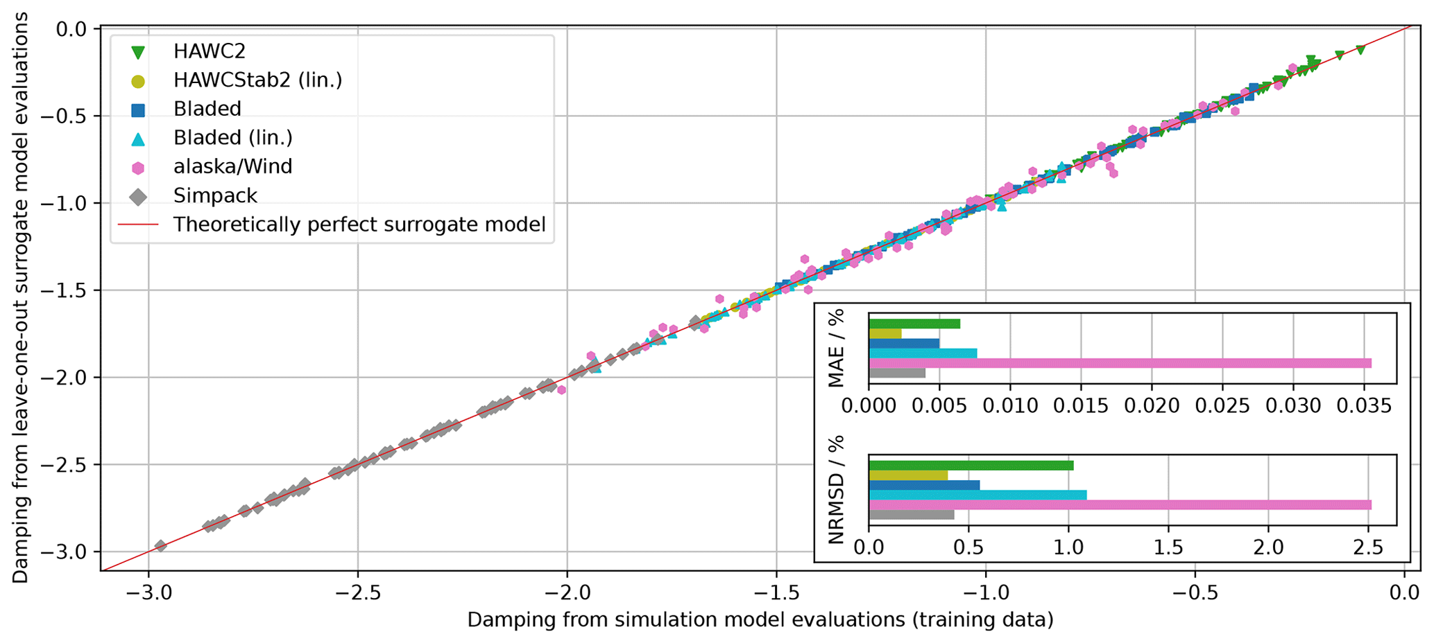
Figure 7 Case study 1: comparison between leave-one-out surrogate model evaluations and training data samples.

3.2.1 PCE model verification

The simulation tools are sampled with the quasi-random Hammersley scheme to generate 72 training data points for the surrogate models. As described in Sect. 3.1.1, a leave-one-out surrogate model is set up for each training data point. This model verifies the accuracy of the surrogate model if the given training data point is excluded from the training data basis. Figure 7 shows the leave-one-out surrogate model evaluations with respect to the training data points. A perfectly accurate representation of the simulation model by the leave-one-out surrogate model would result in the points lying on the straight line (red line in Fig. 7). Satisfying agreement is found for all tools. The error metrics defined in Sect. 3.1.1 are visualized in the bottom right of Fig. 7. The mean absolute error (MAE) is a measure of the accuracy of the surrogate model to represent the training data. It has the same unit as the QoI, in this case the absolute damping ratio. The normalized root mean square deviation (NRMSD) expresses its accuracy normalized by the bandwidth of damping values. The MAE figure shows that most surrogate models represent the training data with an error smaller than 0.01 % damping. The alaska/Wind surrogate model has the largest error. Nevertheless, the MAE is smaller than 0.04 % damping and the relative error is approximately 2.5 %, which is still very small and almost negligible.

3.2.2 UQ results

The first-order and total Sobol indices are shown in Fig. 8. The main finding is equivalent in all tools. The torsional stiffness has the highest contribution towards the damping of the critical edgewise mode. The fact that the first-order and total Sobol indices are nearly identical implies that the interaction among the uncertain parameters is not significant.

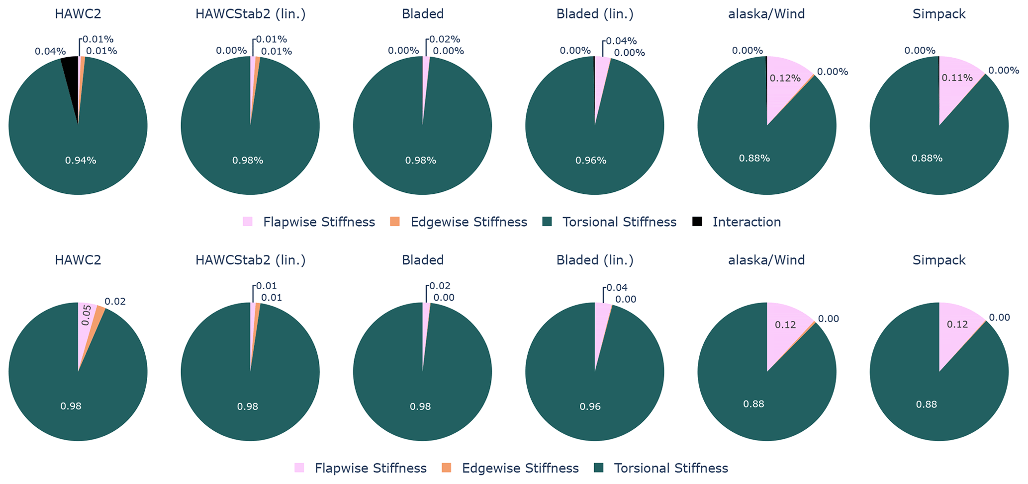
Figure 8 Case study 1: first-order Sobol indices – isolated uncertainty contribution of the investigated parameters (top row), total Sobol indices – uncertainty contribution of the investigated parameters including interactions with other parameters (bottom row).

Two noticeable differences should be pointed out. Firstly, HAWC2 is the only model where the interaction between the uncertain parameters has a noteworthy contribution (4.12 %). Secondly, the sensitivity of the flapwise stiffness is significantly higher in Simpack and alaska/Wind compared to the other tools.

Figure 9 gives a more intuitive and simultaneously more detailed view on the first-order effect of the isolated parameters. Each of the uncertain parameters is varied from its minimum to maximum value while keeping the other parameters constant at their mean value. This visualizes a single slice of the full uncertainty domain. The conclusions from the first-order Sobol indices in Fig. 8 (top row) correlate well with the results in Fig. 9. The dominating sensitivity of the torsional stiffness is clear from the strong gradient (right panel). In all tools the damping increases for an increasing torsional stiffness. The gradients of this sensitivity are overall similar, yet the curves for some tools are nonlinear, with locally highly different trends between the tools. The flapwise stiffness variation plot shows the sensitivity of the damping in Simpack and alaska/Wind. Here one can also conclude that the overall gradient is similar, but the nonlinear trend is opposite. The sensitivity in Simpack seems to have a nonlinear convex shape, while the sensitivity in alaska/Wind has a nonlinear concave shape.

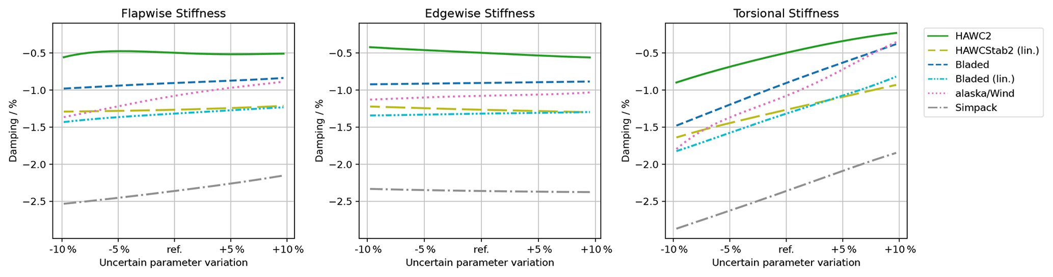
Figure 9 Case study 1: first-order effects of an isolated parameter (other parameters at reference value) .

3.3 Case study 2: manufacturing defects

This case study was proposed to demonstrate a possible use case in the actual wind turbine development process and to show the comparability of the tools for more intricate uncertain parameters.

The edgewise stiffness, principal axis orientation, position of the center of gravity, and position of the shear center along the chord are used as uncertain parameters. These beam properties are known to be sensitive to manufacturing defects and assumed to have a significant impact on the stability. Noever-Castelos et al. (2021) investigated the influence of realistic manufacturing defects of the beam properties on the SmartBlades2 DemoBlade. The Gaussian distributions of these beam properties were scaled to the IWT reference blade, while retaining similar distributions along the blade. This approach is not intended to be exact or to result in a generally valid conclusion. Rather, it was attempted to use uncertainty distributions with physical meaning instead of using arbitrary academic values.

3.3.1 PCE model verification

The leave-one-out verification and corresponding error metrics are shown in Fig. 10. The correlation is again satisfying in all tools. The largest dispersion and therefore highest error metrics can be seen for the Bladed linearization. The NRMSD is relatively high, with a maximum error of approximately 9 % for the Bladed (lin.) model. This is caused by the small bandwidth between maximum and minimum values, which is used to normalize the error. The small bandwidth implies that even a small error has a rather large normalized error. The MAE is in this case a better error indicator. For all tools the MAE remains below 0.015 % damping.

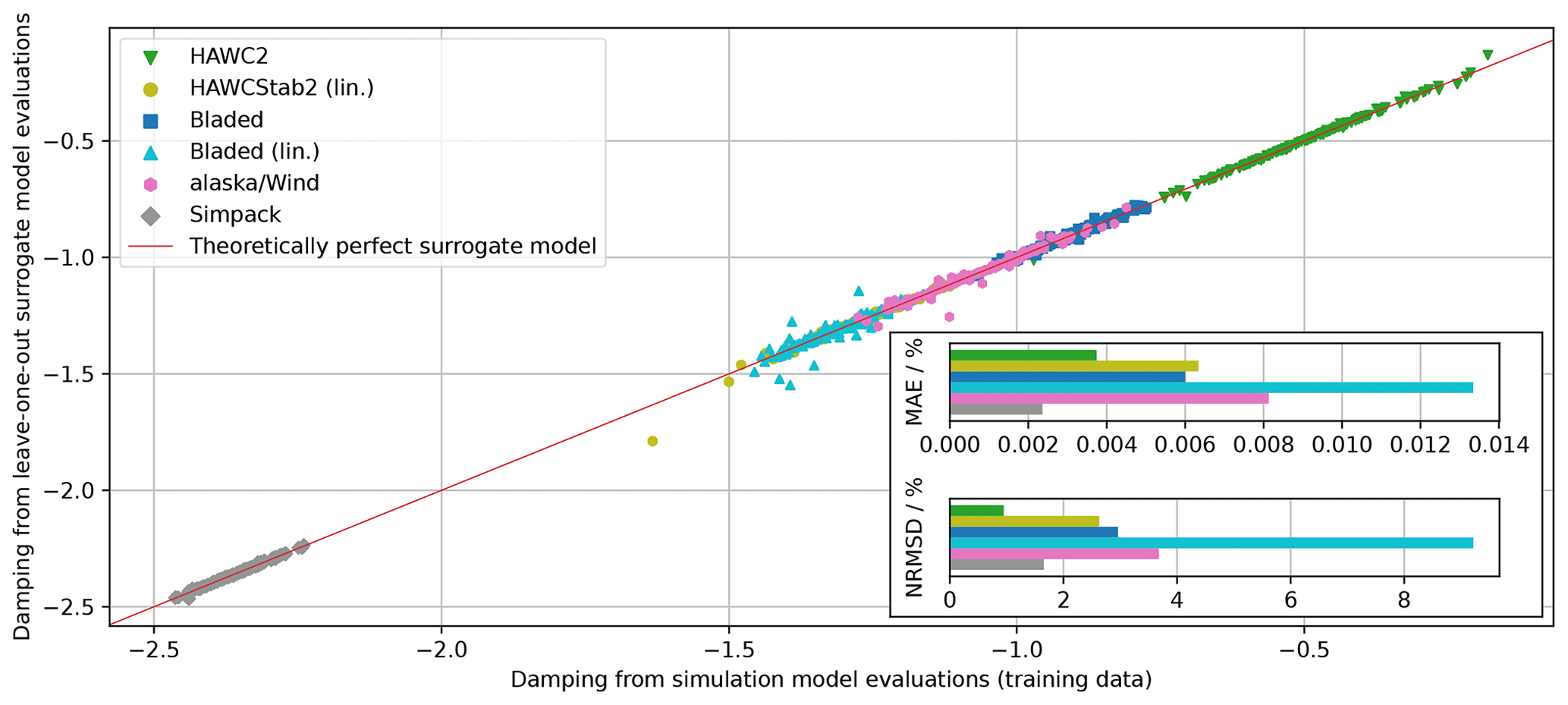
Figure 10 Case study 2: comparison between leave-one-out surrogate model evaluations and training data samples.

3.3.2 UQ results

The first-order and total Sobol indices for case study 2 are shown in Fig. 11. Major differences in the uncertainty quantification appear. Overall, the chordwise COG and chordwise shear center position have the highest sensitivity. However, which of these two has the dominant uncertainty contribution varies with the tools. HAWC2 and HAWCStab2 show a dominating uncertainty contribution by the chordwise shear center position. All other tools show a dominating contribution by the center of gravity position. The orientation of the principal axis has in all tools a negligible influence on the damping. The edgewise stiffness has a significant contribution to the overall variation in HAWC2, HAWCStab2, and Simpack but a negligible contribution in Bladed, Bladed (lin.), and alaska/Wind. Similar to case study 1, the interaction between uncertain parameters has only a limited contribution to the overall damping variation.

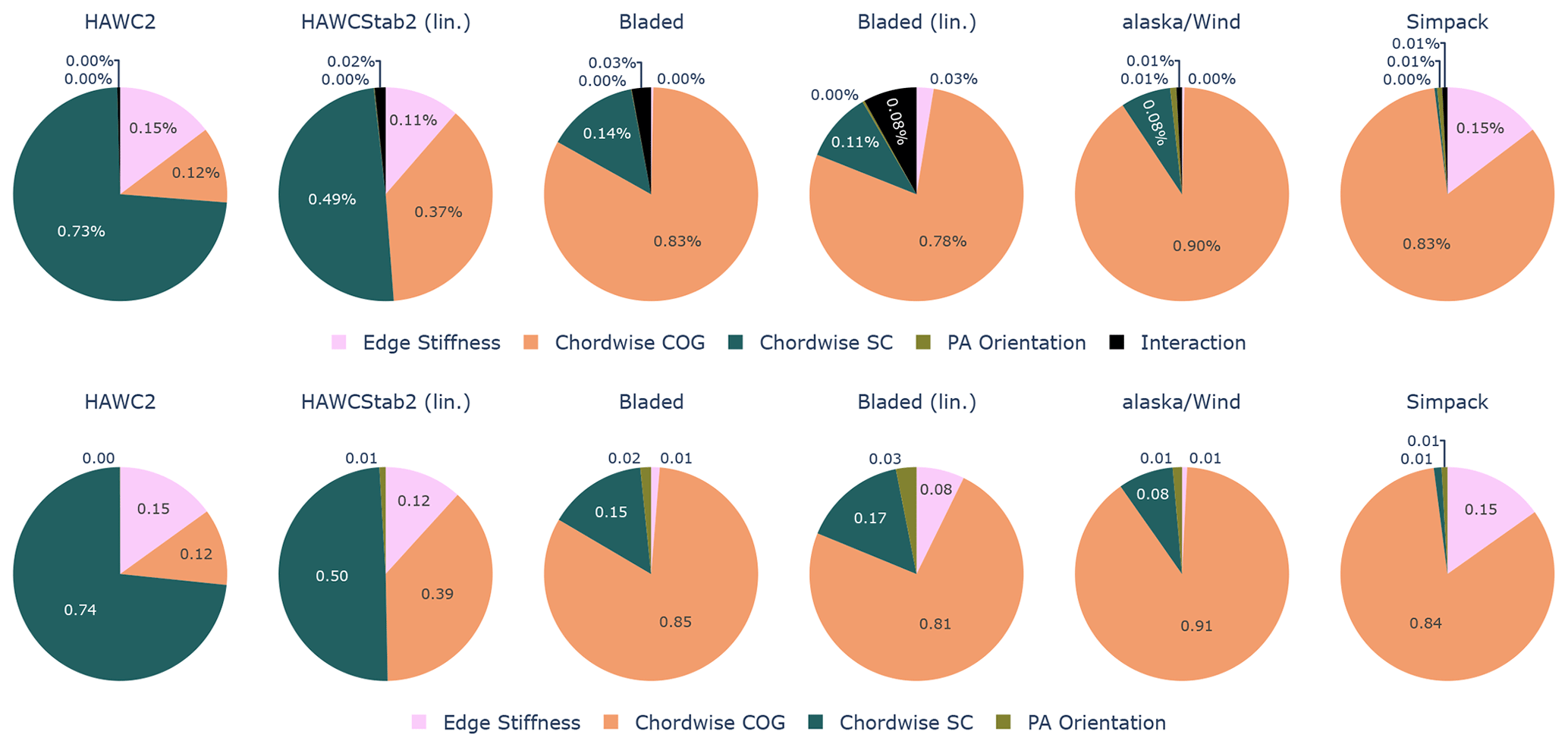
Figure 11 Case study 2: first-order Sobol indices – isolated uncertainty contribution of the investigated parameters (top row), total Sobol indices – uncertainty contribution of the investigated parameters including interactions with other parameters (bottom row).

Figure 12 visualizes the isolated influence of each parameter when all other parameters are kept at their nominal values. The principal axis orientation uncertain parameter is not shown because it has a negligible uncertainty contribution in all tools. Especially interesting is the influence of the chordwise shear center position. In HAWC2 and HAWCStab2 the damping increases significantly if the shear center moves towards the trailing edge, which correlates with the higher Sobol indices seen in Fig. 11. The trends and/or gradients in the other tools are completely different. Note that the uncertain parameter variation in all tools has been verified by comparison of the structural blade eigenfrequencies. The differences which appear here are therefore due to the instability mechanism as a whole. This figure also exposes the limitations of the condensation of the parameter sensitivities to Sobol indices. Bladed, Bladed (lin.), and alaska/Wind have similar Sobol indices for the chordwise SC parameter, yet the dependency of the damping on this parameter appears to be highly different between these tools. The isolated effect of the chordwise COG position is more similar for all tools. All tools show a decrease in damping for a backward-moving COG. In alaska/Wind, the gradient is significantly larger. Increasing the edge stiffness has a destabilizing effect in HAWCStab2, HAWC2, and Simpack but a negligible sensitivity in Bladed, Bladed (lin.), and alaska/Wind.

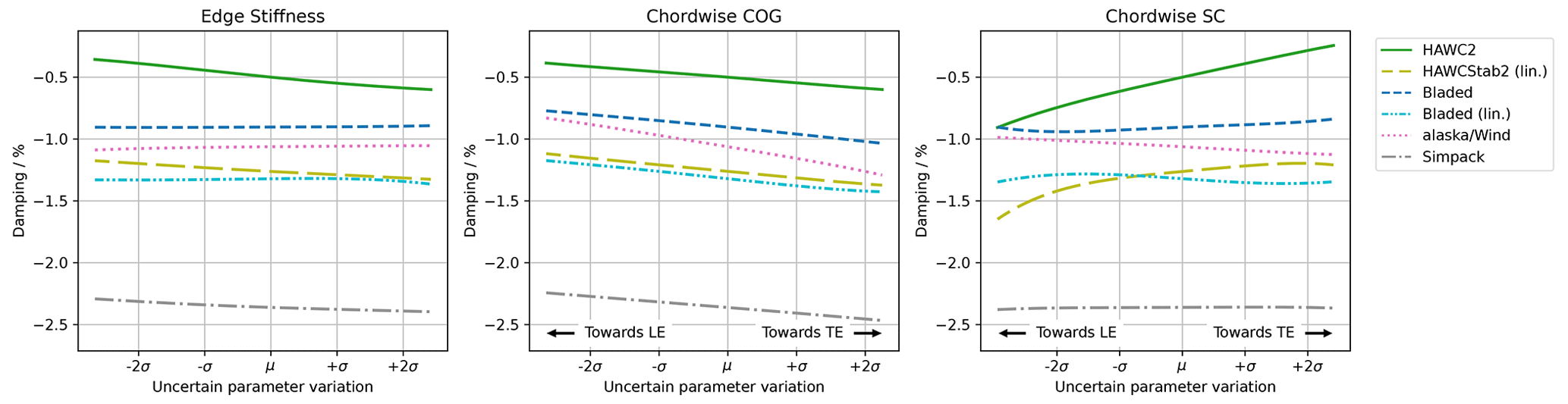
Figure 12 Case study 2: first-order effects of an isolated parameter (other parameters at reference value) .

4 Conclusions

Models for multi-body simulations of wind turbines consist even in the described low-fidelity case of a huge number of parameters describing the degrees of freedom – especially for the blade. Evaluating and understanding the influence of each of these parameters on the aeroelastic stability of the model is complex. Sophisticated uncertainty quantification methods have to be used to assess the sensitivity in both a mathematically rigorous and computationally efficient manner.

In this work a code-to-code comparison between industry-relevant low-fidelity aeroelastic simulation tools (alaska/Wind, Bladed, HAWC2/HAWCStab2, and Simpack) has been done on the sensitivity of beam structural parameters to an edgewise whirling instability. The edgewise whirling instability was established on the IWT reference turbine through a reduction of the blade stiffness. To enable the comparison of time domain and linearization tool results, a dynamic mode decomposition (DMD) post-processing methodology for nonlinear time domain simulation has been introduced. This procedure was tuned for the identification of the unstable modes and should be developed further if it is to be applied to all operating conditions and all aeroelastic modes. The comparison of the reference condition showed overall satisfying agreement between the tools. An accurate match of the frequency of the edgewise modes of the aeroelastic system in the selected operating states could be found in almost all tools. The modal damping showed similar trends over the operating points but noticeable differences in the absolute values. A detailed study of the instability mechanism and the possible differences in the separate tools was out of the scope. Further investigation in this respect could help to understand the differences in damping observed in the Campbell diagrams and the differences in case study 2 of the uncertainty quantification. This study would require an analysis of the complex aeroelastic mode shapes and the net aerodynamic work introduced into or extracted from the system. This analysis is not trivial and would require its own dedicated study, especially considering the variations in capabilities and precision among the different tools.

A PCE surrogate model was used in the uncertainty quantification to reduce the computational cost. The PCE models were successfully verified by means of leave-one-out tests, which proves that these models are well suited to represent the full uncertainty domain. Case study 1 showed equivalent sensitivities in all tools with a dominating influence of the torsional stiffness compared to flapwise and edgewise stiffness. Major differences between the tools appeared in case study 2. The dominating uncertain parameter and the trend of the sensitivities were vastly different. This shows the complexity involved in the aeroelastic stability assessment. Even though the basic aeroelastic properties and the reference stability analysis of the different models appeared very similar, the parameters influencing said instability can still be significantly different for different tools. In both case studies, the interaction between the uncertain parameters was limited, which would imply that the uncertainty quantification could have been done at equal accuracy but significantly lower computational cost. It is important to note that the results of both case studies have to be understood within the assumptions of this work. The results will depend on the presented simulation models, the fixed operating conditions, the instability mechanism itself, and the selection and definition of the uncertain parameters and quantity of interest. The generalization of these results is difficult and should be made with caution. The case studies only covered a small number of uncertain parameters. In the future, it would be interesting to extend this to other, also non-structural, parameters. Furthermore, the input uncertainty distributions should be based on realistic deviations, e.g., known uncertainties due to manufacturing imperfections or degradation over its lifetime.