Impact of a two-dimensional steep hill on wind turbine noise propagation

Wind turbine noise propagation in a hilly terrain is studied through numerical simulation in different scenarios. Linearized Euler equations are solved in a moving frame that follows the wavefront, and wind turbine noise is modeled with an extended moving source. We employ large-eddy simulations to simulate the flow around the hill and the wind turbine. The sound pressure levels (SPLs) obtained for a wind turbine in front of a 2D hill and a wind turbine on a hilltop are compared to a baseline flat case. First, the source height and wind speed strongly affect sound propagation downwind. We find that topography influences the wake shape, inducing changes in the sound propagation that drastically modify the SPL downwind. Placing the turbine on the hilltop increases the average sound pressure level and amplitude modulation downwind. For the wind turbine placed upstream of a hill, a strong shielding effect is observed. But, because of the refraction by the wind gradient, levels are comparable with the baseline flat case just after the hill. Thus, considering how terrain topography alters the flow and wind turbine wake is essential to accurately predict wind turbine noise propagation.

1 Introduction

The increase in demand for renewable energy and the low power density characteristic of wind energy have led to the development of extended wind farms. A significant barrier to the successful implementation of these installations is noise annoyance, which often leads to diminished public acceptance (Gaßner et al., 2022). Hence, accurate models for noise prediction from single wind turbines and wind farms are necessary to extend the use of wind energy. In recent years, significant efforts have been made to characterize wind turbine noise. This includes the study of the wind turbine inflow, noise emission mechanisms, and the effect of the propagation medium on the far-field noise level. Aerodynamic noise, which is caused by the interaction of the incoming wind with the blades of the turbines, is dominant, broadband, and can propagate over several kilometers (Van Den Berg, 2004; Hansen et al., 2019). The main origins of aerodynamic noise are turbulent inflow noise and trailing edge noise (Oerlemans et al., 2007). The movement of the blades induces amplitude modulation (AM), which is considered to be one of the main annoyance issues (van den Berg, 2005; Hansen et al., 2019). The noise production is greatly influenced by the geometry of the blades and by the incoming wind profile and turbulence characteristics. Several models have been developed to predict wind turbine noise emission. Point source approaches are commonly utilized (Lee et al., 2016; Prospathopoulos and Voutsinas, 2007). However, more sophisticated methods considering an extended aeroacoustic sound source have also been developed (Cotté, 2019; Bresciani et al., 2024; Cao et al., 2020).

These approaches enable more accurate modeling of the flow and the geometry's impact on sound levels and AM prediction. Atmospheric conditions affect wind turbine noise propagation, prompting the development of various numerical methods to study these effects. They are generally based on propagating sound through already-generated flow fields, either analytically or numerically. Predictions of wind turbine noise propagation using a parabolic equation model or particle-based approach have been compared against field experiments (Könecke et al., 2023; Nyborg et al., 2023). Barlas et al. (2018) and Heimann and Englberger (2018) have studied the influence of wind velocity and temperature profiles on noise generation mechanisms and noise propagation. An important finding is that the wind turbine wake can act as a waveguide and create a focusing zone near the ground. Its position and intensity notably depend on the velocity deficit of the wind turbine wake. One of the main results (Barlas et al., 2017b; Heimann and Englberger, 2018) is that far-field AM is greatly influenced by wind shear and turbulent intensity and that focusing zones (their existence, intensity, and position) strongly depend on small variations in the meteorological conditions.

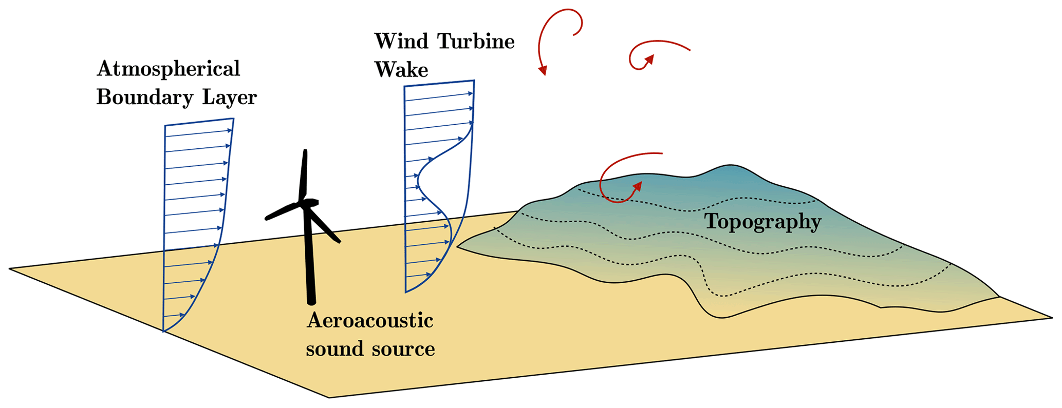
Besides atmospheric refraction, factors such as topography and ground absorption also affect long-range sound propagation, as demonstrated in Fig. 1. Placing wind turbines on hilltops is common due to the improvement in energy production (Berg et al., 2011). Therefore, in such configurations, considering the topographical effects on noise production and propagation becomes essential (Elsen and Schady, 2021). The influence of a 3D hill on both the flow around the wind turbine and the noise propagation has been studied by Heimann et al. (2018). In their work, the atmospheric flow perturbed by the hill and the wind turbine is computed using large-eddy simulation (LES). The results are then used as an input for propagation simulations using a 3D ray-based sound particle model. The authors show that positioning the wind turbine on the hilltop can reduce the overall sound pressure level (OASPL) in the far field. This can compensate for the amplification on the ground due to the wake, which tends to enhance the OASPL further downstream. Shen et al. (2019) studied topography effects for a realistic case considering a wind farm over a complex ground. They used a 2D parabolic equation method to propagate sound over long distances and account for topography and flow effects (Sack and West, 1995; Nyborg et al., 2023). The noise levels were compared with those for flat ground considering either a homogeneous atmosphere at rest or a logarithmic mean velocity profile. Both the topography and the turbulent flow characteristics were shown to be key components in predicting noise propagation. Despite these studies, the combined effect of the flow and topography on sound propagation is not yet fully understood. Indeed, noise levels in the far field are strongly dependent on parameters like the position of the sources, hill shape, and atmospheric boundary layer (ABL) conditions, which makes it difficult to draw a general conclusion on the effect of topography. Moreover, the impact of the turbine's position relative to the hill is largely unexplored, and the effects of atmospheric flow conditions on the interplay between sound production and propagation remain unclear.

This work aims to address these last two points and further investigate the phenomena present when considering wind turbine sound propagation with topography. Hence sound propagation is simulated for several positions of a single wind turbine relative to a 2D hill, i.e., a ridge. The position of the wind turbine relative to the hill is expected to have an impact both on the flow around the wind turbine, especially the development of the wake, and on sound propagation directly, through reflection, refraction, and scattering of acoustic waves. Here only a single hill and wind turbine geometry are considered to showcase the strong influence of topography on sound propagation. To study these phenomena, a propagation method based on linearized Euler equations (LEEs) (Colas et al., 2023) is used. The effects of the hill and the wind turbine on the flow are taken into account through the mean flow values obtained from LES performed in the work of Liu and Stevens (2020). LEE methods are not widely used for the long-range propagation of wind turbine noise because they are computationally demanding. Here the use of LEEs is relevant as more classical methods based on geometrical acoustics or parabolic equations could be limited in the presence of topography.

Figure 1 Sketch of the main wind turbine noise propagation factors.

The paper is organized as follows. In Sect. 2, the methodology is briefly described. Then the cases studied and the numerical simulations performed are presented in Sects. 3 and 4. The propagation effects are first described in Sect. 5.1. Then the SPL fields for the complete wind turbine are compared between the different cases in Sect. 5.2. Finally, we compare our results with previous studies in Sect. 6 and give concluding remarks in Sect. 7.

2 Methodology

2.1 Wind turbine noise model

The methodology employed to compute wind turbine noise involves three steps as depicted in Fig 2. It is similar to the methodology described in Colas et al. (2023) and is only briefly summarized here. First, LES with an immersed boundary method (Gadde et al., 2021; Gadde and Stevens, 2019; Stieren et al., 2021; Stevens et al., 2018) is used to determine the average flow field. Although the simulations are unsteady, only the mean velocity fields are utilized in this study, disregarding turbulence scattering despite its known influence on wind turbine noise propagation. Scattering by turbulence could lead to a less efficient focusing by the wind turbine wake and to an increase in sound pressure level in shadow zones. This effect was previously studied in Barlas et al. (2017b), and they show that utilizing the average flow fields yields AM and average OASPL that are similar to those obtained with a fully unsteady simulation. It is not clear if these observations still hold for cases with topography.

Figure 2 Diagram of the complete wind turbine noise prediction methodology.

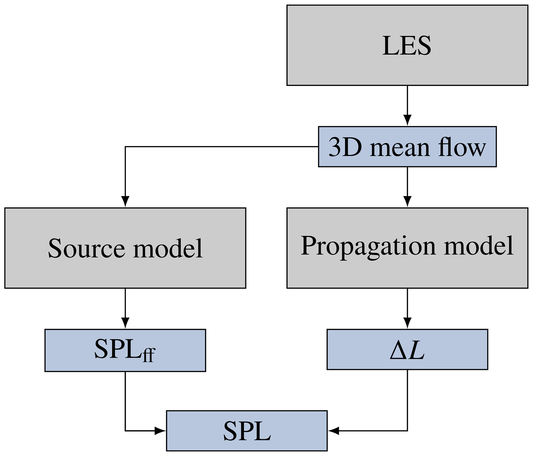
The wind turbine noise is computed using the moving monopole (MM) approach proposed by Cotté (2019). First, the SPL in the free field, denoted SPL_ff, is computed using Amiet's strip theory (Amiet, 1976). Each blade is divided into several segments, regarded as uncorrelated point sources. Then, the trailing edge noise and turbulent inflow noise are calculated considering the blade geometry and input mean flow, for each segment at each angular position (Tian and Cotté, 2016; Mascarenhas et al., 2022). Note that this model is only valid in the far field (distances larger than the blade chord and the wavelength). The SPL at a receiver is finally computed by adding the effect of atmospheric absorption and the relative sound pressure level, denoted ΔL, which encompasses the ground and refraction effects on the sound propagation. It writes

$$\begin{array}{}\text{(1)}& {\mathrm{SPL}}^i(\mathbf{x},f,\mathit{\beta })={\mathrm{SPL}}_{\mathrm{ff}}^i(\mathbf{x},f,\mathit{\beta })+\mathrm{\Delta }{L}^i(\mathbf{x},f,\mathit{\beta })-\mathit{\alpha }\left(f\right)R,\end{array}$$

where i is the segment index, x is the receiver coordinates, f is the frequency, β is the blade angle (with β=0 corresponding to the blade pointing upward; see Fig. 7), α is the atmospheric absorption coefficient, and R is the distance from the source to the receiver. In this case, ΔL is computed using 2D LEE simulations, described in the next section, but other propagation models could be employed, such as parabolic equation methods, ray tracing (see Sect. 5.1.3), or engineering models. To decrease computational expenses, ΔL is not calculated for every segment position. Instead, fictive source heights are assumed along a vertical line in the rotor plane that passes through the turbine's hub. Hence ΔLⁱ in Eq. (1) corresponds to a linear interpolation of the computed values of ΔL between the two closest fictive sources. Finally, the SPL produced by the wind turbine is obtained by summing the contributions of all blade segments of the three blades:

$$\begin{array}{}\text{(2)}& \mathrm{SPL}(\mathbf{x},f,\mathit{\beta })=\mathrm{10}{\log }_{\mathrm{10}}\left(\sum _{i=\mathrm{1}}^{\mathrm{3}{N}_{\mathrm{s}}}{\mathrm{10}}^{{\mathrm{SPL}}^i(\mathbf{x},f,\mathit{\beta })/\mathrm{10}}\right),\end{array}$$

where N_s is the number of segments per blade. The SPLs are integrated for a set of frequencies from 50 Hz to 1 kHz (Colas et al., 2023) to retrieve the OASPL:

$$\begin{array}{}\text{(3)}& \mathrm{OASPL}(\mathbf{x},\mathit{\beta })=\mathrm{10}{\log }_{\mathrm{10}}\left(\sum _{i=\mathrm{1}}^{N_{\mathrm{f}}}\mathrm{\Delta }{f}_i{\mathrm{10}}^{\mathrm{SPL}(\mathbf{x},f_i,\mathit{\beta })/\mathrm{10}}\right),\end{array}$$

where N_f is the number of computed frequencies, and Δf_i is the bandwidth. Finally, the averaged OASPL ($\stackrel{\mathrm{‾}}{\mathrm{OASPL}}$) and AM are computed over one rotation such that

$$\begin{array}{}\text{(4)}& \begin{array}{rl}{\displaystyle }& {\displaystyle }\stackrel{\mathrm{‾}}{\mathrm{OASPL}}\left(\mathbf{x}\right)=\mathrm{10}{\log }_{\mathrm{10}}\left(\sum {\mathrm{10}}^{\mathrm{OASPL}(\mathbf{x},\mathit{\beta })/\mathrm{10}}/N_{\mathit{\beta }}\right),\\ {\displaystyle }& {\displaystyle }\mathrm{AM}\left(\mathbf{x}\right)=\underset{\mathit{\beta }}{max}\left(\mathrm{OASPL}\right(\mathbf{x},\mathit{\beta }\left)\right)-\underset{\mathit{\beta }}{min}\left(\mathrm{OASPL}\right(\mathbf{x},\mathit{\beta }\left)\right),\end{array}\end{array}$$

where N_β is the number of angles discretizing the rotor rotation.

2.2 Propagation model

The propagation model is based on the numerical solution of the LEEs, which are solved in a 2D curvilinear mesh to account for topography. The 3D effects, meaning horizontal refraction induced by the wind speed gradient perpendicular to the propagation direction, are neglected due to the 2D approximation. This approximation is common in outdoor sound propagation, but 3D effects may have an influence, especially near the wake, and should be addressed in future work. A set of two equations is derived from the LEE for atmospheric acoustics without source terms (Ostashev et al., 2005):

$$\begin{array}{}\text{(5)}& \begin{array}{rl}& {\displaystyle \frac{\partial p}{\partial t}}+{\mathbf{V}}_{\mathbf{0}}\cdot \mathrm{\nabla }p+{\mathit{\rho }}_{\mathrm{0}}{c}_{\mathrm{0}}^{\mathrm{2}}\mathrm{\nabla }\cdot \mathbf{v}=\mathrm{0},\\ & {\displaystyle \frac{\partial \mathbf{v}}{\partial t}}+({\mathbf{V}}_{\mathbf{0}}\cdot \mathrm{\nabla })\mathbf{v}+(\mathbf{v}\cdot \mathrm{\nabla }){\mathbf{V}}_{\mathbf{0}}+{\displaystyle \frac{\mathrm{\nabla }p}{{\mathit{\rho }}_{\mathrm{0}}}}=\mathrm{0},\end{array}\end{array}$$

where p and $\mathbf{v}=(u,w)$ are the acoustic pressure and velocity, ρ₀ is the mean density, ${\mathbf{V}}_{\mathrm{0}}=(u_{\mathrm{0}},w_{\mathrm{0}})$ is the mean velocity, and c₀ is the sound speed. Note that here u₀ corresponds to the projection of the horizontal wind speed on the propagation direction. A conservative formulation of this system of equations is then derived for the transformation of the coordinate system from Cartesian to curvilinear. The same curvilinear transformation as in Colas et al. (2023) and originally proposed by Gal-Chen and Somerville (1975) is employed to follow the terrain elevation. A Gaussian pulse introduced as an initial condition is used to represent a broadband monopole (Colas et al., 2023). Equation (5) is solved with high-order optimized finite-difference techniques (Bogey and Bailly, 2004; Berland et al., 2006). To simulate a realistic ground, a broadband impedance condition (Troian et al., 2017) is implemented at the bottom of the domain, and a convolutional perfectly matched layer (CPML) simulates unbounded propagation at the top of the domain (Cosnefroy, 2019; Petropoulos, 2000). The acoustic variables and the boundary conditions are computed in a moving frame that follows the wavefront. This greatly reduces the computational cost as the propagation distance is large (around 15000 acoustic wavelengths). This method is described in Emmanuelli et al. (2021) and Colas et al. (2023).

From the time domain solution, it is possible to recover a frequency domain solution. ΔL can be derived from the time signal p(t) recorded at one receiver such that

$$\begin{array}{}\text{(6)}& \mathrm{\Delta }L(f,\mathbf{x})=\mathrm{10}{\log }_{\mathrm{10}}\left({\displaystyle \frac{\left|P\right(f,\mathbf{x}){|}^{\mathrm{2}}}{\left|P_{\mathrm{ff}}\right(f,\mathbf{x}){|}^{\mathrm{2}}}}\right),\end{array}$$

where P is the Fourier transform of p, and P_ff is the free field solution, i.e., the solution for the same source term but without any mean flow or ground reflection. ΔL for each third-octave band f_c is computed by averaging over the broadband results.

3 Cases studied

This work focuses on three configurations that were previously studied by Liu and Stevens (2020) for a truly neutral ABL, which corresponds to a pressure-driven ABL where no temperature effects are modeled. For each configuration, LES is performed with and without the turbine inside the flow. These cases are referred to as X_WT (with the wind turbine) and X_ABL (without the wind turbine). This allows one to investigate topographic effects on sound propagation isolated from wake effects. The configurations are defined as follows:

• cases A_ABL and A_WT, baseline case of a wind turbine with flat ground;

• cases B_ABL and B_WT, a wind turbine placed upstream of a 2D hill;

• cases C_ABL and C_WT, a wind turbine placed on top of a 2D hill.

The hill considered for cases B and C is defined such that

$$\begin{array}{}\text{(7)}& h\left(x\right)=h_{\max }{\cos }^{\mathrm{2}}\left({\displaystyle \frac{\mathit{\pi }x}{\mathrm{2}l}}\right),-l\le x\le l,\end{array}$$

where h_max=100 m and l=260 m. Note that x=0 corresponds to the turbine position. Hence the hill is shifted between cases C and B (see Fig. 5); x=0 corresponds to the beginning of the hill in case B and to the hilltop in case C.

The velocity fields are normalized by the friction velocity u_*. This scaling is well-accepted within the framework of this model. However, it is important to acknowledge that it does not account for more detailed atmospheric effects, such as atmospheric stability, which can significantly impact flow profiles (Stoevesandt et al., 2022). Two friction velocities are considered such that the wind speed at z=100 m is equal to u_ref=8 m s⁻¹ and u_ref=10 m s⁻¹, which are typical values for wind turbine applications. The diameter and height of the turbine are set to 100 m, and the roughness height at the ground is 0.01 m, which is representative of flow over smooth terrain. As we consider neutral conditions, the temperature is assumed to be constant throughout the domain. The variable-porosity model is used to model the ground impedance (Attenborough et al., 2011). The effective flow resistivity is set to 50 kNs m⁻⁴, and the effective porosity change rate is set to 100 m⁻¹, which reflect natural soil conditions (Cotté, 2018).

Figure 3 LES mean flow velocity fields for the baseline cases (a) A_ABL without and (b) A_WT with the wind turbine. See Fig. 4 for the y–z plane view.

Figure 4 Case A_WT: mean flow from LES in the y–z plane at positions (a) $x=-\mathrm{100}$ m, (b) x=0 m, (c) x=100 m, and (d) x=200 m, with x=0 m being the turbine's location. See Fig. 3 for the x–z plane view.

The side view of the streamwise mean velocity is plotted in the plane of the wind turbine's hub in Fig. 3 for cases A_ABL and A_WT (note that for conciseness only the results for u_ref=10 m s⁻¹ are presented in this section). When a wind turbine is present, the velocity deficit that occurs downstream requires several hundred meters to recover. The shape of the wake can also be observed in the y–z plane at different downstream positions in Fig. 4. It presents a circular zone with a few meters per second velocity deficit just after the wind turbine, which progressively fades away further downstream of the wind turbine.

Figure 5 Mean flow velocity field for cases (a) B_ABL, (b) B_WT, and (c) C_ABL.

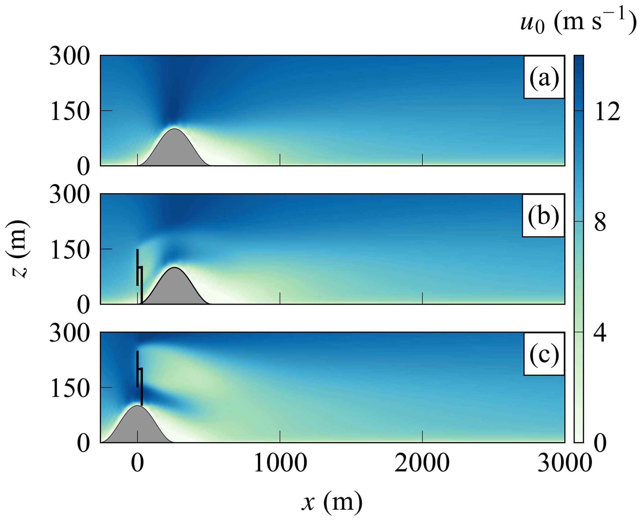
In the presence of the hill, the flow is first shown without the wind turbine in Fig. 5a. An increase in speed is observed at the hilltop as the flow accelerates around it. A recirculation zone is then created downstream of the hill, which leads to the reduction in the mean velocity toward negative values. With the wind turbine in front of the hill (Fig. 5b), the wake of the turbine follows the shape of the hill, counterbalancing the increase in wind speed at the hilltop. Hence the hill's wake appears to be longer and higher. With the wind turbine on the hilltop (Fig. 5c), its wake is larger and mixes with the hill's wake.

Profiles of the streamwise mean velocity are plotted for cases A_WT, B_WT, and C_WT in Fig. 6 at different distances from the wind turbine to better show the effect of the hill. For all cases, the velocity deficit has a top-hat shape for the first few hundred meters downwind of the turbine due to the actuator disk model (Stevens and Meneveau, 2017; Bastankhah and Porté-Agel, 2014). Then, as the ABL flow recovers, a Gaussian shape seems more accurate in describing the wake. Another interesting observation is the influence of the topography on the wake shape. For case B_WT (Fig. 6b), the wake goes up and then down to follow the shape of the hill. The wind speed gradients at the top and bottom of the wake are smaller than for the baseline case A_WT (Fig. 6a). For case C_WT (Fig. 6c), the turbine's wake moves down to follow the topography. The wind gradients and velocity are stronger in this case because of the flow acceleration on top of the hill. These changes in the wake shape and intensity are expected to also influence sound propagation.

Figure 6 Mean flow velocity profiles at different positions x from −10 m to 2.5 km for cases (a) A_WT, (b) B_WT, and (c) C_WT. For case C_WT, the wind turbine is on the hilltop; hence the first three profiles stop before z=0.

The noise emitted by the turbine depends on the inflow conditions and hence varies for each case. The wind speed profile used as an input for the model is taken 10 m upwind of the turbine. The turbulent dissipation rate is set to ϵ=0.01 m² s⁻³, which is a classical value for a neutral atmosphere (Muñoz-Esparza et al., 2018). The rotational speed is defined from the wind speed at hub height using the relation described in Jonkman et al. (2009). Finally, the twist of each blade segment is set to obtain an optimal angle of attack (4° for the considered airfoil) with respect to the wind speed at hub height and the rotational speed (Tian and Cotté, 2016). An equivalent overall sound power level (OASWL) can be estimated for each case. It is computed from the downwind sound pressure level in the free field according to

$$\begin{array}{}\text{(8)}& \mathrm{OASWL}={\mathrm{OASPL}}_{\mathrm{ff}}\left(R\right)+\mathrm{10}{\log }_{\mathrm{10}}\left(\mathrm{4}\mathit{\pi }{R}^{\mathrm{2}}\right),\end{array}$$

where R is the distance between the hub and the receiver taken to be equal to 3 km in this case. Note that for large enough R (more than 1 km), the OASWL becomes constant. The wind speeds are slightly different between the baseline case A (u_hub=10 m s⁻¹) and case B (u_hub=9.5 m s⁻¹). This is an effect of the hill's blocking, which slightly decelerates the flow upstream. This induces a small decrease in the rotational speed Ω and consequently a slight decrease of 0.6  dBA in the OASWL. Case C, on the other hand, shows a significant increase in wind speed (25 % compared to A_WT) and rotational speed (8 % compared to A_WT) due to the elevated hub and the increased wind speed at the top of the hill. Consequently, the OASWL increases by 2 dBA compared to case A. These results are summarized for each case in Table 1.

Table 1 Wind turbine source parameters calculated for each case.

4 Numerical setup for the propagation simulations

For each case presented in Sect. 3, numerical simulations of the noise propagation are performed using the LEE method described in Sect. 2.2. The moving frame has a length of 300 m × 300 m. The grid step is set to $\mathrm{\Delta }x=\mathrm{\Delta }z=\mathrm{0.05}$ m, and the CFL (Courant–Friedrichs–Lewy) number is set to 0.5. These numerical parameters produce accurate results up to 1 kHz. The results are then computed in the frequency domain and presented averaged in third-octave bands.

Figure 7 Sketch of the computational domain. β is the blade angle, and τ is the propagation angle.

First, the simulations are performed in a 3D domain using an N×2D approach. The sound propagation is computed in vertical planes as described in Sect. 2, neglecting transverse propagation effects. The 2D simulations are performed for a set of angles of propagation τ (Fig. 7), to compute a ΔL map around the wind turbine. The flow is almost symmetrical with respect to the x axis; hence only angles between 0° and 180° are considered. This set of simulations is computed only for the source at the hub height (100 m) and for a wind speed u_ref=8 m s⁻¹. The 3D rectangular domain has a size of 4 km × 2 km ×300 m as illustrated in Fig. 7. To capture all significant propagation effects, sound propagation is simulated up to 3 km downwind and up to 1 km in the crosswind and upwind directions. Hence, the angular step must be smaller for the computations downwind of the wind turbine. For τ between 0 and 15°, a 2° angular step is used, and an angular step of 5° is used for the rest of the domain. This is done to save computational resources as a 1 km propagation simulation takes around 240 CPU hours, and a full simulation (with all propagation angles) takes around 2×10⁴ CPU hours. The ΔL fields obtained from these simulations are presented in Sect. 5.1.1.

A second set of simulations is performed only in the downwind (τ=0°) and upwind (τ=180°) directions for the six cases with u_ref=10 m s⁻¹. Here, several source heights are considered to compute the OASPL and AM using the MM approach (see Sect. 2). The wind turbine considered is the same as in Colas et al. (2023). Seven source heights are considered for all cases except for case C_WT in the downwind direction where 30 source heights are used to reach convergence of the AM results. The comparison between the two wind speeds is shown in Sect. 5.1.2, and the OASPL and AM obtained from the six cases are compared in Sect. 5.2.

5 Results and discussion

5.1 Propagation effects

5.1.1 General case description

Figure 8 shows ΔL fields for the six considered cases at f_c=800 Hz on the planes y=0 and z=2 m. The reference cases without wind turbines are on the left, and the results with wind turbines are on the right. For all cases, a point source is placed 100 m above the ground, which corresponds to the hub height. Without the wind turbine and with flat ground (Fig. 8a), the flow varies only along the vertical direction. Upwind it corresponds to a negative effective sound speed gradient that is responsible for the shadow zone observed in cases A_ABL and A_WT. Sound waves are refracted upward as they propagate, leading to a zone with very low SPL at the ground for $x<-\mathrm{500}$ m. The positive effective sound speed gradient downwind refracts sound waves downward and can lead to an increase in SPL at the ground (Barlas et al., 2018; Heimann and Englberger, 2018). For case A_ABL (Fig. 8a downstream of the turbine), the gradient does not produce strong focusing because the velocity gradient is small for a neutral ABL.

Figure 8 ΔL field at f_c=800 Hz for the six cases studied (b, d, f) with and (a, c, e) without the wake in the mean flow. The source is at $x=y=\mathrm{0}$ and z=100 m (circle), and the wind speed at 100 m is equal to 8 m s⁻¹.

The velocity gradient induced by the wake (case A_WT) has a significant effect on sound propagation (Fig. 8b). As shown in previous studies by Barlas et al. (2017b) and Heimann and Englberger (2018), the wake from a wind turbine has a significant impact on the SPL observed at ground level. This effect is clearly visible when comparing Fig. 8a and b. The wake, created by the wind turbine's downstream velocity deficit, acts as a waveguide that causes sound waves to focus at a point approximately 3 km away from the noise source. Note that this focusing effect occurs for small propagation angles only (τ≈0) and that for higher angles of propagation, the ΔL field is similar to the one without the wake. This emphasizes the importance of considering the wake when studying sound propagation in such scenarios.

The hill impacts sound propagation in two ways: directly, by causing reflections and diffraction of the sound waves due to the terrain, and indirectly, by altering the average airflow patterns. Hence, the effect of the wake presented for cases A_ABL and A_WT can be either strengthened or counterbalanced by the influence of the terrain. In the case of the wind turbine positioned upstream of the hill (Fig. 8c, d), most of the propagation effects can be attributed to the hill itself, and the wind turbine wake has a minimal impact. The primary effect is the shielding effect of the hill that creates a shadow zone downwind. A secondary effect is the ΔL amplification that can be observed at x=700 m at ground level. It is caused by the strong velocity gradient created by the hill's wake. However, even with this refraction by the mean flow, the shielding effect of the hill on sound propagation is strong. Hence, ΔL is negative after the hill, except for this focusing zone. Cases B_ABL and B_WT present the same upwind shadow zone as in cases A_ABL and A_WT, which shows that the hill has almost no influence on the upwind propagation. The velocity gradient induced by the wake itself is small in comparison to the hill's wake (see Fig. 5b). Hence, the waveguide effect that was observed for case A_WT is not visible. This indicates that the effect of the wake created by a turbine placed upstream of a hill is overshadowed by the effect of the hill itself. Note that a stronger effect of the turbine's wake is visible when considering increased source heights.

When the wind turbine is located on the hilltop (Fig. 8e, f), the geometry of the hill first creates a cusp caustic just above the bottom of the hill (at x=260 m). The caustic then separates into two branches, one going directly up and one reflecting toward the ground at 330 m. This is only an effect of the terrain and can be observed for both cases C_ABL and C_WT. On the top view, the caustic branch hitting the ground moves further away from the hill as the propagation angle increases. This is equivalent to propagation over a hill with a smaller slope angle, for which the caustic is created higher, and the downward-refracted branch hits the ground further away from the hill's base. The second focusing effect visible for case C_ABL (Fig. 8e) is similar to what is observed in case B. The diminished wind speed behind the hill creates a focal area at the ground positioned at x=1300 m. However, this effect is less noticeable than in case B due to the more pronounced direct influence of the source. For case C_WT (Fig. 8f) the wind turbine wake induces different focusing patterns, somewhat similar to those that are visible in case A_WT. Note that the focusing patterns induced by the flow and hill depend on the source height and wind velocity. Hence they are further studied in the following sections.

5.1.2 Effect of wind speed

In this section, the effect of the velocity on propagation is briefly examined. The previous results were obtained for a wind profile characterized by a wind speed at 100 m equal to u_ref=8 m s⁻¹. In general, a wind turbine operates at wind speeds between 6 and 25 m s⁻¹ (Jonkman et al., 2009). Hence, additional simulations are run for cases A_WT and C_WT with u_ref equal to 10 m s⁻¹ to assess the effect of the wind speed on the refractions. The ΔL contour plots at 800 Hz for cases A_WT and C_WT are compared for both wind speeds in Fig. 9. The general dynamics are similar for both wind speeds, but the focusing effect is enhanced for u_ref=10 m s⁻¹. With flat terrain, the steeper vertical velocity gradient guides sound waves more efficiently toward the ground, resulting in a greater ΔL, especially between 2500 and 3000 m.

Figure 9 ΔL field at f_c=800 Hz for cases (a, b) A_WT and (c, d) C_WT, with (a, c) u_ref=8 m s⁻¹ and with (b, d) u_ref=10 m s⁻¹. The source is at 100 m from the ground (circles).

The ΔL values for receivers at 2 m above the ground are presented for the two wind speeds in Fig. 10. The wave focusing created by the wake induces a maximum after x=2000 m in the ΔL values for all cases. The effect of the caustic at the bottom of the hill is also present for case C with a strong peak at x=300 m. The change in wind speed has a similar effect on ΔL for case A_WT and case C_WT. By increasing the wind speed the focusing phenomenon intensifies: the peak is stronger and more localized. There is a 1.5 dB increase between u_ref=8 m s⁻¹ and u_ref=10 m s⁻¹ for case A_WT and a 0.5 dB increase for case C_WT. As the wind speed increases, the ΔL upstream of the focusing zone decreases for case A_WT (between x=1000 m and x=1800 m). This is explained by the fact that less energy is redirected outside of the focusing area as the amplification becomes stronger and more localized. The focusing zone on the ground also appears closer to the source. For case C, the maximum shifts 250 m closer to the source at 10 m s⁻¹ compared to the case at 8 m s⁻¹. A small shift in the focusing induced by the hill's wake is also noticeable at x=700 m. Oppositely, the focusing induced by the hill geometry at x=520 m does not appear to be shifted by the change in wind speed.

Figure 10 ΔL at 2 m height at f_c=800 Hz for cases A_WT and C_WT, for u_ref=8 m s⁻¹ (dashed lines) and u_ref=10 m s⁻¹ (solid lines)

To summarize the above, with increasing wind speed, the focusing effect intensifies and moves closer to the source where sound pressure attenuation due to geometrical spreading and atmospheric absorption is lower. The wind turbine noise production also increases at higher wind speeds. Both effects lead to an increase in SPL. Hence, in the following only the case where u_ref=10 m s⁻¹ is studied.

5.1.3 Effect of source height

The influence of the source height on sound propagation is crucial for the prediction of wind turbine noise. In the model considered in this work, the rotational motion of the blades is translated into a vertical motion of the sources. Hence, sound propagation depends on the source position, which impacts locations where sound amplification at the ground is observed. In addition, the position of the focusing zone changes with source height. This section aims to gain some insights into the different propagation effects and their dependence on source heights.

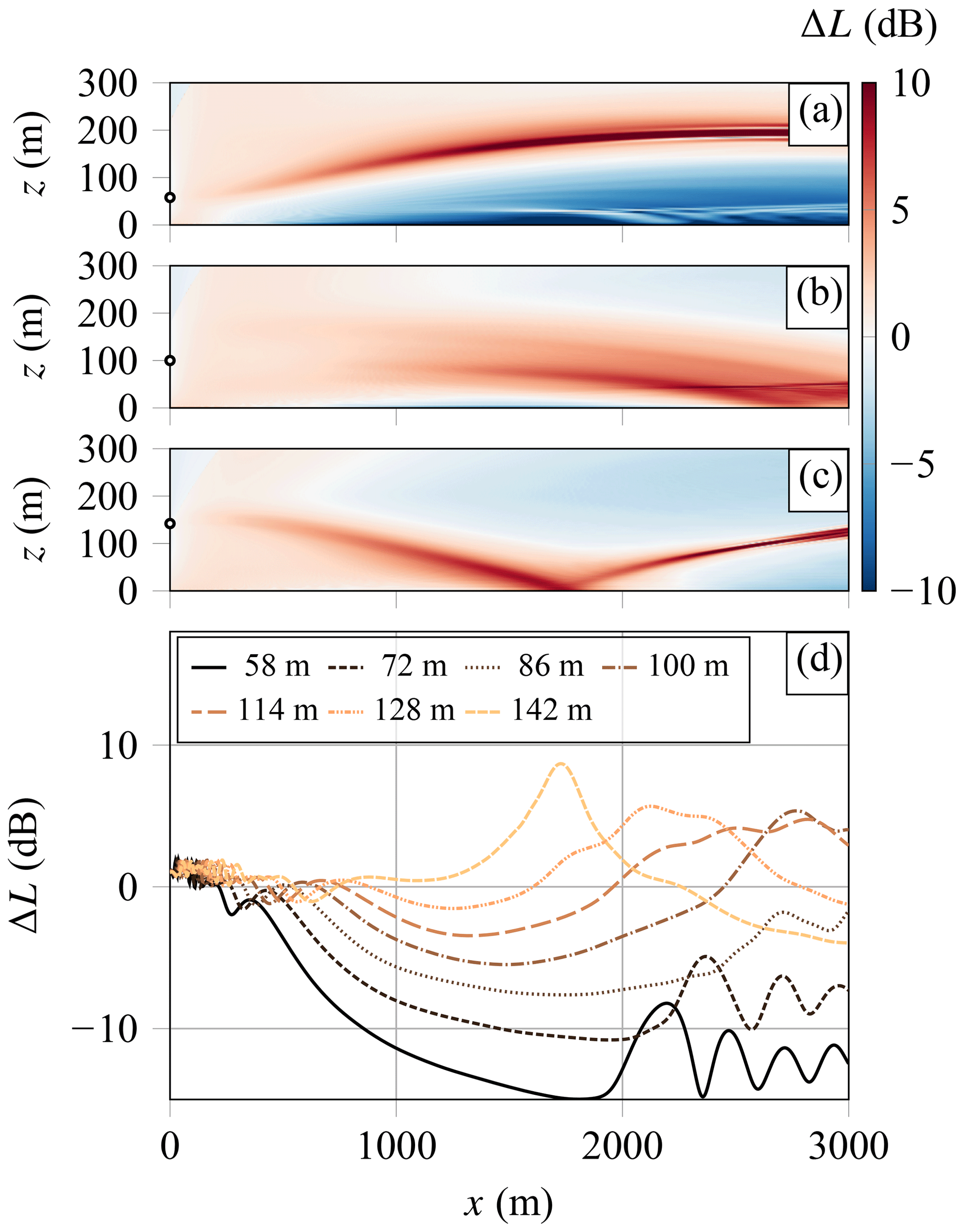
Figure 11 ΔL field at f_c=1000 Hz for case A_WT for three different source heights: (a) h_s=58 m, (b) h_s=100 m, and (c) h_s=142 m; (d) ΔL at 2 m above the ground for the seven source heights.

The ΔL computed for case A_WT for three source heights is shown in Fig. 11a, b, and c; Fig. 11d shows the ΔL for a line of receivers at z=2 m for the seven source heights considered. Three different focusing effects can be observed. For a source height h_s=58 m (Fig. 11a), the sound waves are first refracted upward by the bottom of the wake, then, after the wake recovery, the sound waves are redirected toward the ground by the positive vertical velocity gradient in the ABL. For h_s=100 m (Fig. 11b), two focusing zones can be observed: one at the bottom of the wake and one at the top. They reach the ground after 2.5 km, leading to an increase over a larger surface at the ground. This is similar to what was found in Barlas et al. (2017b). Finally, for h_s=142 m (Fig. 11c), only one focusing zone created by the top-wake gradient is observed. Here, the top-wake positive gradient effectively redirects sound waves toward the ground. Figure 11d shows the differences in SPL at the ground induced by these focusing patterns. For the highest source, a clear peak is present at x=1700 m. As the source height decreases the peak gets wider, is less pronounced, and moves downstream. Finally, when the source is too close to the ground, the focusing occurs at a higher altitude and does not reach the ground before x=3000 m.

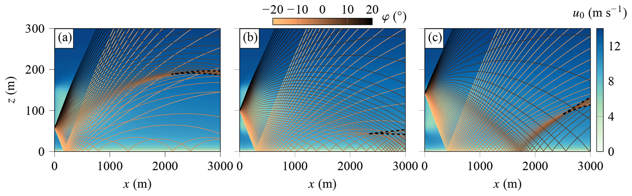
Figure 12 Atmospheric refraction in case A_WT displayed using a ray-tracing method for three different source heights: (a) h_s=58 m, (b) h_s=100 m, and (c) h_s=142 m. The rays are superimposed over the wind speed fields u₀, φ is the initial elevation angle of each ray, and caustics are shown in dashed black lines.

The effect of the flow and in particular the wake on sound propagation appears to strongly depend on the source heights. To validate and provide an additional explanation for the findings in Fig. 11, a ray-tracing simulation is conducted (Candel, 1977; Scott et al., 2017). The ray paths are shown superimposed on the velocity fields in Fig. 12 for elevation angles φ between −20 and 20°. The flow gradient bends the rays, leading to focal areas called caustics. These caustic curves (shown in dashed black lines) delimit a region in which the number of rays increases. The caustic curve itself corresponds to high sound pressure locations. First, note that both prediction methods give identical results for the position of the focusing zones. The caustic positions in Fig. 12 match with regions of high ΔL levels in Fig. 11.

In addition, the ray-tracing approach provides information on the path taken by the sound waves that leads to this increase in ΔL. For the highest source (Fig. 12c), the rays launched at small positive angles are strongly redirected toward the ground by the positive shear at the top of the wake. As the source moves downward, the rays launched upward travel a greater distance before being redirected downward by the wake; hence the focusing zone reaches the ground farther from the source. For sources that are sufficiently low (Fig. 12a and b), the rays launched downward are first refracted upward by the bottom-wake negative gradient before being refracted downward by the positive ABL shear. For h_s=100 m (Fig. 12b), both phenomena occur. The rays launched upward are refracted downward by the top-wake positive gradient, and the rays launched at negative angles are redirected toward the ground but less efficiently due to the bottom-wake negative velocity gradient. Note that this method allows us to precisely show the refraction effect of the wind shear but has limitations when it comes to computing precise SPL as it is a high-frequency approach.

Figure 13 ΔL field at f_c=1000 Hz for case C_WT for three different source heights: (a) h_s=170 m, (b) h_s=185 m, and (c) h_s=248 m; (d) ΔL at 2 m above the ground for seven source heights.

The same type of analysis can be performed for case C_WT. The ΔL fields are again plotted for three source heights in Fig. 13a, b, and c. In Fig. 13d the ΔL values are plotted for seven source heights ranging from h_s=152 m to h_s=248 m. The source heights 215, 230, and 248 m correspond to the situation shown in Fig. 13c, in which only one focusing zone is present, similar to case A_WT. With decreasing source height, the focusing zone shifts away from the source. When the sources are located at 185 and 200 m, two distinct peaks appear, which correspond to the two focusing zones visible in Fig. 13b. These two peaks start to merge as the source approaches the ground (see Fig. 13a). Consequently, for source heights between 152 and 176 m, the ΔL at the ground shows a more complex pattern because the two focusing zones are superimposed. The cusp caustic at the bottom of the hill is observed for the three source heights in Fig. 13a, b, and c. The corresponding increase in ΔL is also visible in Fig. 13d between x=250 m and x=500 m. These peaks move closer to the base of the hill for sources close to the ground.

Figure 14 Atmospheric refraction in case C_WT displayed using a ray-tracing method for three different source heights: (a) h_s=170 m, (b) h_s=185 m, and (c) h_s=248 m. The rays are superimposed over the wind speed fields u₀, φ is the initial elevation angle of each ray, and caustics are shown in dashed black lines.

To better understand the source height influence on the focusing pattern, the ray-tracing results are again shown in Fig. 14 for the three source heights. For h_s=170 m two caustic branches match the ΔL increase observed in Fig. 13a. The wake induces a convergent beam of rays, creating a cusp caustic. This caustic may correspond to the one observed in case A_WT in Fig. 12, but here, due to the geometry of the wake, the branches hit the ground before 3 km. As the source height increases (Fig. 14b), two focusing zones appear. In this case, the rays launched toward the ground are not refracted upward anymore but are only deviated by the bottom of the wake. There is no caustic before the bottom-wake focusing hits the ground. The second focusing zone is induced by the top-wake gradient. Finally, for h_s=248 m (Fig. 13c), the behavior is similar to what is shown for case A_WT where the rays are strongly refracted by the wake gradient at the top and only this effect dominates.

Through the analysis of cases A_WT and C_WT, we saw that the wind turbine wake has a strong influence on the propagation. More precisely, the focusing pattern is modified by the source heights because sound waves are refracted differently by the wind turbine wake. The effect of the source height on case B_WT is not presented here as the focusing induced by the wind turbine wake in this case hits the ground far away from the source with low intensity. Nevertheless, the amplification position moves with source height, as for cases A_WT and C_WT, inducing some AM in the far field, as presented in the following section.

5.2 Wind turbine noise

In this section, the OASPL due to the wind turbine is analyzed. We start by discussing the OASPL results from a single blade. Next, we compare the OASPL, averaged over one full rotation, and AM for a wind turbine with three blades for all six cases.

5.2.1 One-blade OASPL

First, snapshots of the OASPL obtained for one blade for case C_WT are presented for six different blade angles in Fig. 15. For all the following plots the near field where the source model is not valid is shown with a gray area. The far field is defined in this work such that $\left|x\right|>\mathrm{10}\times c_{\mathrm{0}}/f_{min}=\mathrm{70}$ m, where $f_{min}=\mathrm{50}$ Hz. This yields distances much larger than the wave length and the wind turbine blade chord length. The effects of the source model and the propagation are visible. The OASPL is higher close to the source and decreases as the receiver moves further away due to geometrical spreading and atmospheric absorption. In addition, the flow and topography effects described in the previous section are still visible. The dependence of OASPL on blade orientation comes from the activation of different ΔL fields (Sect. 5.1.3) as the blade moves up and down. The blade starts upward on the snapshot at the top, with the focusing hitting the ground at x=1800 m. Then the blade moves downward to β=180°, and the focusing zone reaches the ground at around x=3000 m. The blade finally moves upward again, and the focusing zone moves back toward the source. The source height also influences the OASWL, as the wind speed is higher at z=148 m than at z=52 m. This evolution of OASWL is responsible for AM close to the source, while the change in propagation path induces AM in the far field as the peak positions at the ground are modified. This effect was shown in Heimann et al. (2018) with the particles emitted from the lower sources being refracted upward and those emitted from the highest sources being refracted downward. These phenomena are also visible for cases A_WT and B_WT and are shown in the next section.

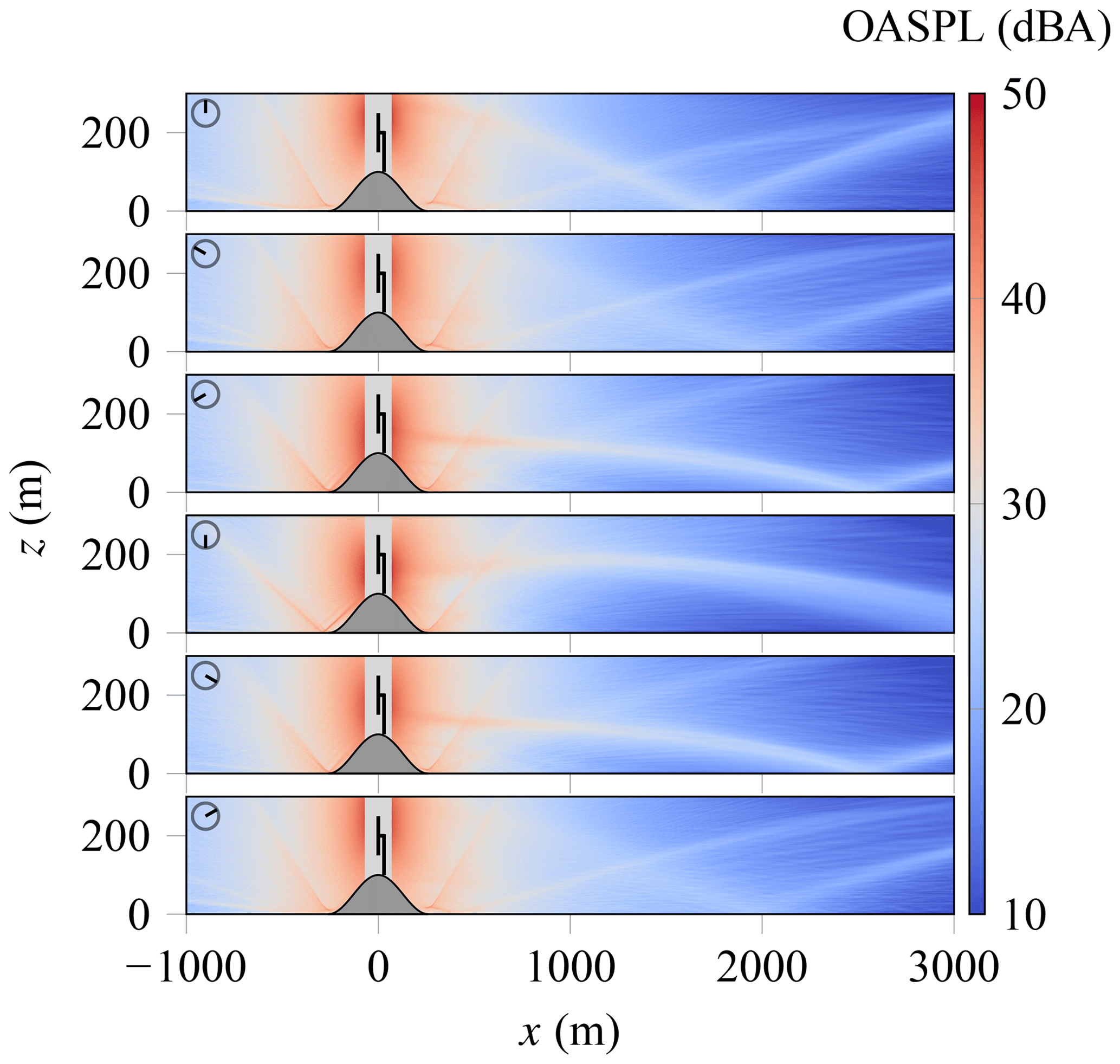
Figure 15 OASPL for case C_WT for one blade at different angular positions (indicated in the top-left corner).

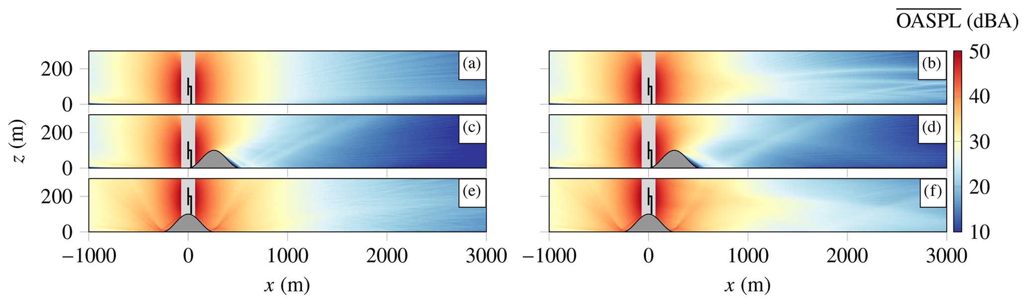
Figure 16 Averaged OASPL over one rotation for the six cases with and without the wake. (a) A_ABL, (b) A_WT, (c) B_ABL, (d) B_WT, (e) C_ABL, and (f) C_WT.

5.2.2 Averaged OASPL and AM

The OASPLs averaged over one rotation are shown in Fig. 16 for the six cases and a velocity at z=100 m of 10 m s⁻¹. By summing the contribution of the three blades and averaging over one rotation, the focusing effects previously described tend to average out for all cases. The OASPL does not increase downwind when the wind turbine wake is not in the flow (Fig. 16a, c, and e). The shadow zone is distinguishable upwind close to the ground for cases A_ABL and B_ABL. Figure 16c shows the focusing zone induced by the hill's wake in case B_ABL. Finally, in Fig. 16e, caustics at the bottom of the hill in case C_ABL are present on both sides. As previously shown, focusing patterns appear downwind for cases accounting for the wake (Fig. 16b, d, f). Even for case B_WT, where the shielding effect of the hill is strong, sound waves appear to be redirected toward the ground at a great distance. Hence, an increase in OASPL downwind at the ground is expected for these cases.

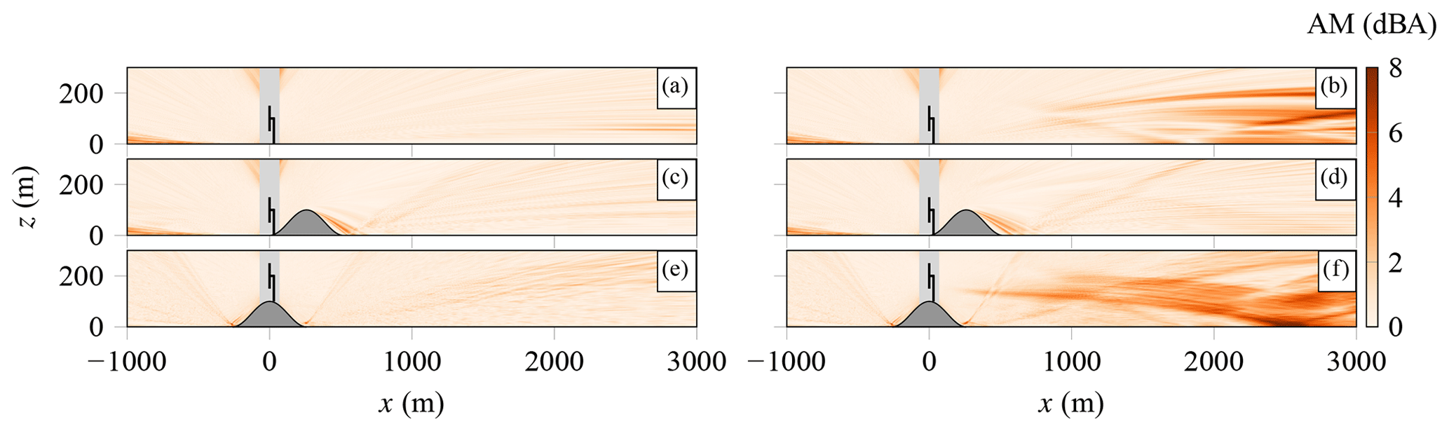
Figure 17 AM for the six cases with and without the wake. (a) A_ABL, (b) A_WT, (c) B_ABL, (d) B_WT, (e) C_ABL, and (f) C_WT.

Corresponding AM fields are shown in Fig. 17. The AM is very low for all cases without the wake. It can be concluded that downwind and upwind AM is not significantly affected by the OASWL variation due to blade rotation. Other authors have also reached this conclusion (Cotté, 2019). The AM would increase crosswind as the source moves closer to and farther from the receiver (Cotté, 2019; Barlas et al., 2017a; Mascarenhas et al., 2023). The AM increases close to the ground for $x<-\mathrm{500}$ m for cases A and B due to the upwind shadow zone. For cases B_WT and B_ABL, the zone with large AM after the hill corresponds to the focusing induced by the hill's wake. An important result is that no AM is present downwind for the cases without the wake (Fig. 17a, c, e). On the other hand, the variation in focusing patterns in cases A_WT and C_WT leads to strong AM downwind (Fig. 17b, f).

The comparison of the average OASPL is presented in Fig. 18a for receivers at 2 m height. Case A_ABL shows a downwind decrease mostly due to the atmospheric absorption and the geometrical decay. Upwind, the shadow zone becomes discernible at $x=-\mathrm{700}$ m with a steeper decrease. The downwind OASPL is higher in case C_ABL with a consistent difference of 5 dBA with case A_ABL. Note that 2 dBA is due to the increase in OASWL, and the remaining 3 dBA comes from propagation effects. Upwind, the shadow zone moves away from the source as the wind turbine is higher. For case B_ABL the shielding of the hill downwind induces a strong dip between 250 and 600 m. However, the OASPL at the focus zone (x=700 m) is of comparable amplitude with the SPL of the other cases at this position. Hence, although the hill shields the noise, levels remain significant at ground level just after the shadow zone. Downwind of the focusing zone, the levels are 4 dBA lower than for case A_ABL. In this case, 0.6 dBA is lost at noise emission. In the upwind direction, (x<0), case A and case B are almost equivalent as there is no effect of the topography or the mean flow on sound propagation.

Figure 18 Comparison of (a) the OASPL and (b) the AM at 2 m above the ground between the six cases.

The main effect of the wake on the OASPL is an increase downwind at ground level. The wake seems to have a similar effect on the average OASPL for cases A_WT and C_WT. The average OASPL increases by 4 dBA for x>1700 m, which corresponds to the closest focusing zone shown in Figs. 11 and 13. For case B_WT, a similar increase can be observed but farther from the source (x > 2200 m). It is worth noting that these results differ from those obtained when using a point source approximation where the focusing zone is more localized (Colas et al., 2022). In this previous study, it was found that case A_WT could show higher OASPL in the far field than case C_WT.

Finally, the corresponding AM values are presented in Fig. 18b. Upwind there is almost no influence of the wake. For cases A and B, a clear increase in AM at $x=-\mathrm{700}$ m is visible. It corresponds to the start of the shadow zone. At this distance, the receiver moves in and out of the shadow zone as the blades move up and down, hence yielding AM (Cotté, 2019). For case C, the shadow zone starts further away due to the increased source height. The peaks in AM at x=260 m and $x=-\mathrm{260}$ m are created by the caustics at the bottom of the hill. Downwind, it is clear that for all cases the AM levels are much higher when the wake is present. This is similar to what was found in Heimann et al. (2018) and Barlas et al. (2017b). Case A_WT presents an AM increase up to 4 dBA with maxima at around x=1700 m and x=2200 m with a strong dip at x=1900 m. This shape is a consequence of the superposition of the three blades. As one blade rotates, the focusing zone moves farther from and closer to the source. But because of the contribution of the three blades, there is always an amplification at x=1900 m, corresponding to a source height around hub height. This creates a zone where the OASPL does not vary and hence where the AM is low. The same behavior is visible for case C_WT with even stronger AM (up to 9 dBA). Two dips are distinguishable in this case, as it was shown that two different focusing zones are created when the source height is around hub height (see Sect. 5.1.3). For case B_WT, AM is also present in the far field but does not reach values higher than 2 dBA. For case B, another zone of AM is visible at x=600 m for both case B_WT and case B_ABL. This increase by 4 dBA comes from the refraction induced by the hill's wake.

We recover some well-known effects of wind turbine sound propagation, such as downwind amplification induced by the wind turbine wake and upwind AM created by the negative effective sound speed gradient (Mascarenhas et al., 2023; Barlas et al., 2017b; Heimann et al., 2011). With the turbine on a hilltop, both the noise levels and the AM are greatly increased downwind compared to the flat terrain case. This could result in increased annoyance and is a combined effect of the hill and wind turbine wake. With the wind turbine upstream of the hill, a strong shielding effect reduces the noise level downwind. Nonetheless, levels comparable to the baseline flat case were found just after the hill because of refraction induced by the hill's wake.

6 Discussion

In this section, we aim to compare our results with those from previous numerical studies. For the flat terrain case, our conclusion is in good agreement with the results from Barlas et al. (2017b). The effect of wind speed and source height is very similar in both studies. The increase in wind speed brings the amplification zone closer to the source, and the peaks are sharpened (see Fig. 6 in Barlas et al., 2017b). Likewise, the source height impacts the refraction downwind, and the focusing zone is observed closer to the turbine for a higher source (see Fig. 9 in Barlas et al., 2017b). The effect of the wake on the OASPL downwind of the turbine is also very similar. Barlas et al. (2017b) found that the wake increases the average OASPL for x>1000 m and z=2 m by 5 dB (see Fig. 13 in Barlas et al., 2017b). This is slightly closer to the source than in our results (the increase starts at around x=1700 m), but this can be explained by the increased wind speed at hub height and the smaller wind turbine in their study.

Barlas et al. (2018) also studied AM evolution with distance for varying atmospheric stability. For the neutral case, AM increases downwind with a maximum just before x=1500 m. Again, this is slightly closer to the source than what we found, but this can also be attributed to the wind turbine being smaller in their study. They also found several maximums associated with different refraction patterns induced by different blade positions. The dip in the AM pattern is less pronounced in their study because an unsteady approach was used. AM is not equal to zero in this area, contrary to our findings, as the flow and hence the propagation path vary even when the blade position is identical.

Heimann et al. (2011) showed the importance of 3D sound propagation in the context of wind turbine noise. Two important effects are not accounted for in our study. The spanwise wind speed gradient creates sound wave refraction in the horizontal direction, which is not represented in our model. The wind veer also impacts propagation, inducing an asymmetric SPL distribution. Despite these differences, the two studies can be compared for a flat terrain scenario. They found an increase in average OASPL starting from x > 1000 m, with various patterns depending on atmospheric stability. This is closer to the source compared to our results, even though the wind turbine dimensions and wind speed at hub height are the same. The use of different wind speed profiles and wake models could explain this discrepancy.

Our results for a wind turbine on a hilltop also differ from those reported in Heimann et al. (2018). In their study, the hill and wake effects tend to compensate for each other, while in our work the highest OASPL is obtained for the case with the hill and the wind turbine wake accounted for. There are several explanations for these two opposite conclusions. First, their study does not account for the increased sound emission, while, in our case, the OASWL is higher for case C_WT. But even if changes in sound emission are neglected, we saw that propagation effects contribute to an increase in SPL compared to the flat terrain case. However, it is difficult to assess which propagation effect is responsible for this difference. The propagation distance considered in Heimann et al. (2018) is much smaller, and most of our conclusions are based on results farther than 1 km downwind. Additionally, the hill height in our study is larger. However, due to atmospheric refraction, this does not necessarily imply that the zone of amplification would be located further from the source. Finally, the wake shape is different between the two studies, and, despite having a similar effect, it is not clear if the focusing zone should be different.

7 Conclusions

This study demonstrates that terrain topography can significantly affect wind turbine sound propagation. We used linearized Euler equations, solved in a moving computational frame, and an extended source model to simulate sound propagation from a wind turbine in the presence of topography. The combined effect of a 2D hill, i.e., a ridge, and the velocity gradient created by the terrain and the wind turbine was studied for three configurations. First, we recover some well-known effects of wind turbine sound propagation, such as downwind focusing induced by the wind turbine wake and upwind amplitude modulation created by the vertical velocity gradient in the ABL. In the case of a wind turbine on a hilltop, both the sound levels and the AM are greatly enhanced downwind compared to the flat case. This could result in increased annoyance and is mainly an effect of mean flow field modification. In all cases, the far-field AM downwind is created by the wind turbine's wake. When the turbine is placed in front of the hill, we observed that, despite a strong shielding effect from the terrain, SPL just after the hill is comparable to that of the flat case. This is due to focusing induced by the hill's wake, which also increases AM at this location. Hence, it would be possible to encounter cases where annoyance issues are raised despite a supposed shielding effect of topography. In this case, the effect of the wind turbine wake is limited as sound propagation is mainly determined by the geometry of the terrain and the flow around the hill. While the main effects of the topography highlighted in this study are likely to be general, the specifics of our findings may be limited to the particular hill geometry and wind turbine dimension. Further work could focus on comparing different hill heights and slopes relative to the wind turbine hub height and diameter.

Furthermore, we saw that topography also affects sound emission. For a turbine on a hilltop, the sound emitted is higher than in the flat case due to increasing wind speed. For a turbine upstream of a hill, the sound emitted is slightly lower due to the decrease in wind speed before the hill. Finally, we find that the sound-focusing effect becomes more pronounced and closer to the turbine with increasing wind speed and that most of the propagation effects are directly behind the wind turbine (close to τ=0). However, this might be because our study used an N × 2D approach, which does not consider the full 3D sound propagation through the wake. Also, turbulence in the atmosphere can scatter the sound and reduce the focusing effect we observed, but further research is needed to determine to what extent this happens.