Probabilistic surrogate modeling of damage equivalent loads on onshore and offshore wind turbines using mixture density networks

The use of load surrogates in offshore wind turbine site assessment has gained attention as a way to speed up the lengthy and costly siting process. We propose a novel probabilistic approach using mixture density networks to map 10 min average site conditions to the corresponding load statistics. The probabilistic framework allows for the modeling of the uncertainty in the loads as a response to the stochastic inflow conditions. We train the data-driven model on the OpenFAST simulations of the IEA 10 MW reference wind turbine (IEA-10MW-RWT) and compare the predictions to the widely used Gaussian process regression. We show that mixture density networks can recover the accurate mean response in all load channels with values for the coefficient of determination (R²) greater than 0.95 on the test dataset. Mixture density networks completely outperform Gaussian process regression in predicting the quantiles, showing an excellent agreement with the reference. We compare onshore and offshore sites for training to conclude the need for a more extensive training dataset in offshore cases due to the larger feature space and more noise in the data.

1 Introduction

The selection of a suitable site for the installation of a wind farm plays an important role in limiting installation, maintenance, and operational costs, as well as in ensuring a safe operating lifetime of the structure. This process of site assessment or site-suitability study typically involves a thorough analysis of the structural integrity of the wind turbine at locations with different site-specific environmental inputs.

Wind turbine certification consists of a rigorous analysis of various design load cases (DLCs) defined by the International Electrotechnical Commission (IEC 61400-3-1, 2019) using time-domain engineering tools such as OpenFAST (Jonkman, 2013), HAWC2 (Larsen and Hansen, 2007), and BHawC (Couturier and Skjoldan, 2018; Skjoldan, 2011), to name a few. This step does not typically include site-specific certification. To determine if the wind turbine can handle the loads at a specific site, further analysis is required. The first step involves simulating the DLCs on the type-certified rotor–nacelle assembly with a reference tower. If the site is found suitable, subsequent steps include designing a site-specific tower and performing a site-specific certification. While industry-standard engineering tools are necessary for certification simulations, the preliminary site analysis can benefit from data-driven surrogate models to provide quick load estimates. The main objective of this study is to design surrogates that predict the 10 min load statistics, for instance, 10 min damage equivalent loads (DEL^ST), on a fixed-bottom wind turbine using the 10 min statistics of the environmental conditions as input. This is done using a probabilistic approach to also quantify the uncertainty in the loads stemming from stochastic variation in the inflow conditions in the 10 min window.

Modeling the relationship between the DEL^ST and environmental conditions is non-trivial. Fatigue is a multiscale phenomenon that depends on the material composition, composite structure, part dimensions, and dynamic inflow. This makes it challenging to model using low-fidelity physics-based approaches. As a consequence, data-driven surrogate models can be beneficial, as they do not require prior knowledge of the underlying physics and can infer complex relationships from observations alone. Especially in systems where analytical closed-form solutions are intractable or the physical properties cannot be easily modeled (Jiang et al., 2020), data-driven surrogates provide a great advantage. Essentially, a surrogate is a simpler and computationally inexpensive representation of the complex system that emulates the outputs as a function of the inputs. Surrogates are widely used as engineering tools for preliminary design calculations, optimization, or real-time control, where accuracy can be reasonably traded for computational efficiency. The data used by the surrogate as ground truth are often from a computational model but can also consist of real-life measurements.

Site-specific load surrogates are often designed using deterministic data-driven modeling approaches (Sect. 1.2). For a given training dataset $(\mathit{X},Y)=\mathit{\{}{\mathit{x}}^q,y^q\mathit{\}}$, where q=1…n, deterministic models map a set of K input features x∈ℝ^K to the corresponding output y∈ℝ. However, the assumption of a deterministic relationship between inputs and outputs does not hold in our case. For instance, a single value of 10 min mean wind speed can correspond to an infinite number of inflow patterns, resulting in an infinite number of DEL^ST values with a certain probability distribution conditioned on that wind speed. Probabilistic surrogates allow us to model the complete conditional distribution of the DEL^ST. However, the probabilistic surrogate modeling of offshore wind turbine loads has not been extensively studied in the literature. The primary objective of this study is to develop a probabilistic data-driven surrogate that maps 10 min statistics of wind and wave conditions (X∈ℝ⁶) to the corresponding 10 min load statistics including DEL^ST and standard deviation (Y∈ℝ). We introduce a novel framework for load surrogate modeling that reduces training costs by eliminating seed repetitions without sacrificing prediction accuracy. This probabilistic modeling approach allows for uncertainty propagation and quantification, enabling informed decision-making. In this study, we compare the performance of a highly flexible machine learning method, the mixture density network (MDN) (Bishop, 1994), with the widely used Bayesian approach of Gaussian process regression (GPR). The surrogates are tested using the onshore and offshore versions of the IEA 10 MW reference wind turbine. The loads for training the surrogate are calculated using an open-source, multi-fidelity, multi-physics solver called OpenFAST (NREL, 2022; Jonkman, 2013).

1.1 The case for probabilistic reasoning in site-specific load surrogates

During the 10 min period, wind turbines are subjected to randomly varying inflow turbulence and waves, regarding which the surrogate model has no information. For instance, for a given turbulence spectrum, average wind speed, and average turbulence intensity, there are unlimited variations of inflow turbulence patterns that result in equally varied load responses. OpenFAST takes as an input a frozen turbulence field generated by TurbSim using the Kaimal turbulence spectrum inflow model (Kaimal et al., 1972), consisting of stochastic turbulence patterns created using pseudo-number generators initialized by random seeds. Thus, repeated simulations with the same input parameters but different seeds result in different values of output quantities, yielding a multi-valued mapping, highlighted in Fig. 1. On repeating the simulations with sufficient seeds, the load statistics converge towards a value of statistical moments that characterize a random variable, denoted ($Y\mid \mathit{X}=\mathit{x}$). Furthermore, the mean, variance, and skewness of the random variable are functions of the controller actions, wind speed, wave period, and turbulence intensity, among other site conditions. The heterogeneity in the variance of the conditional probability density function (pdf) across different operating conditions is known as heteroscedasticity.

Figure 1 Schematic representation of the multi-valued mapping of the input–output pairs used to train the surrogate.

Deterministic regression models are generally of the type

$$\begin{array}{}\text{(1)}& y=f\left(\mathit{x}\right)+\mathit{\epsilon },\end{array}$$

where f is a deterministic function of the input features, or the conditional average of the target, and $\mathit{\epsilon }\sim \mathcal{N}(\mathrm{0},\mathit{\sigma })$ is the noise component. This framework can only accommodate the conditional statistics of the target. Therefore, when deterministic models are used, the common practice is to convert the multi-valued problem to a single-valued setting. This is done by averaging the response at each sample point over n unique random seeds to approximate quantities such as $\mathbb{E}\left(Y\right|\mathit{X}=\mathit{x})$, $\mathrm{Var}\left(Y\right|\mathit{X}=\mathit{x})$ or the quantiles of $\left(Y\right|\mathit{X}=\mathit{x})$ (Meinshausen, 2006; Koenker and Hallock, 2001).

The main drawbacks of this approach are as follows.

• A finite sampling of input loading due to stochastic representations of wind and waves in time-domain simulations introduces an uncertainty in the turbine's load response. Zwick and Muskulus (2015) and Müller and Cheng (2018) show that the recommendation by the IEC 61400-1 standard to average over a 60 min long simulation or six 10 min long simulations is insufficient to fully converge to the average fatigue loads. Liew and Larsen (2022) similarly concluded that some load channels are more sensitive to the number of seeds, and the average of the tower base moments can be off by around 3 %–4 %, even with n=10. For training surrogates, it is common to run 60 min long simulations and obtain the average response or perform four to ten 10 min simulations over different random seeds to obtain the average response before training the surrogate (Dimitrov et al., 2018; Dimitrov and Natarajan, 2019; Shaler et al., 2022; Slot et al., 2020). The variability in the response with fewer seeds can be interpreted as noise, forcing the surrogate model to interpolate the noise in case of a small dataset or fit the mean of the response when the dataset is large. However, the mean may be wrongly inferred if the response is non-Gaussian. Seed repetitions add a significant computational cost to the data generation phase, especially when dealing with expensive simulations like in the case of floating wind turbines.

• Modern wind turbines are equipped with sophisticated controllers that can result in multi-modal responses in loads. Training the model on the expectation of a multi-modal distribution can misrepresent the actual load pattern, as the average of several correct target samples is not necessarily a meaningful target value.

• Most real-world learning tasks involve datasets with complex patterns of missing features that introduce aleatoric uncertainty. Unlike numerical simulations, seed repetitions cannot be performed on such datasets.

An alternate approach is to use probabilistic regression that models the targets as random variables, $Y:\mathrm{\Omega }\to \mathbb{R}$, with an unknown conditional pdf, $\left(Y\right|\mathit{X}=\mathit{x})$. Probabilistic models provide a framework for informed decision-making by predicting a confidence interval in addition to the most likely response. For instance, the uncertainty in the 10 min DEL^ST can be propagated to the lifetime DELs while also considering the distribution of the wind speeds to design less conservative, site-specific structures. Probabilistic surrogates such as conditional generative adversarial networks and conditional variational autoencoders use latent variables to infer meaningful quantities from data with complex noise distributions (Blei et al., 2017; Yang and Perdikaris, 2019; Kingma and Welling, 2014; Kneib, 2013). Other probabilistic regression approaches like mixture density networks (Bishop, 2006) and generalized lambda distributions (Zhu and Sudret, 2021) use maximum likelihood estimation to infer the conditional distributions in stochastic systems. The probabilistic surrogate modeling approaches can be trained without having to simulate multiple seed repetitions for each operating condition, as they can infer the conditional response based on neighboring samples. Therefore, training time can be significantly shorter compared to existing frameworks. In addition, it provides estimates of uncertainty with respect to loads and a more robust estimate of mean response. Although it is not within the scope of this paper, Bayesian approaches can also be used to differentiate between aleatoric and epistemic sources of uncertainty in the predictions (Olivier et al., 2021; Vega and Todd, 2022; Hlaing et al., 2024). In current design or certification frameworks, there is no requirement for the quantification of the uncertainty of the loads. However, Li and Zhang (2019) have extrapolated the 50-year accumulated fatigue damage in the mooring lines, tower, etc., which could be beneficial for cost reduction when designing the site-specific tower. As we move towards a reliability-based design process in the future, probabilistic surrogates will prove to be useful.

1.2 Previous work

Wind turbine loads, for site-specific analysis and wind farm design, have commonly been approached with deterministic models like standard artificial neural networks (ANNs) (Schröder et al., 2018; Dimitrov, 2019; Shaler et al., 2022). ANNs are extremely powerful and emulate the loads well if the training data have been averaged over a set of inflow turbulence realizations. Shaler et al. (2022) compare the performance of inverse distance weighting, ANNs, radial basis functions, Kriging with a partial-least-squares dimension reduction, and regularized minimal-energy tensor-product splines in a wind farm array and observe the highest R² values for ANNs and the inverse-distance-weighting method. These approaches, however, do not aim to account for or predict the variance of the load response.

Kriging, also known as the standard Gaussian process regression (GPR) (Rasmussen and Williams, 2006), is capable of uncertainty quantification but is restricted only to normally distributed homoscedastic responses. Nevertheless, due to its flexibility and ease of implementation, it is widely used as a load emulator to estimate the fatigue load response in wind turbines (Teixeira et al., 2017; Avendaño-Valencia et al., 2021; Li and Zhang, 2019, 2020). Gasparis et al. (2020) compare GPR to other data-driven methods like linear regression and artificial neural networks for modeling power and fatigue loads, showing a superior performance by the GPR. Similarly, Dimitrov et al. (2018) evaluate importance sampling, nearest-neighbor interpolation, polynomial chaos expansion (PCE), GPR, and quadratic response surface (QRS) to conclude a better performance again by the GPR despite a computational penalty. Slot et al. (2020) provide a thorough comparison of the performance of PCE and GPR for the uncertainty quantification of fatigue loads on NREL's 5 MW reference onshore wind turbine. They conclude the need for a minimum of four random seeds per training sample in the case of GPR to make high-accuracy predictions. They also note that GPR performs better per invested training simulation than PCE.

Further interest in quantifying the variability of the short-term fatigue loads as a function of the input parameters has initiated research into heteroscedastic surrogates. One of the ways to model heteroscedasticity is through replication-based approaches, wherein the simulations at each set of average input conditions are repeated for multiple realizations of the stochastic field to obtain statistical information about the response. Murcia et al. (2018) use 100 turbulent inflow realizations at each sample point to obtain the first two moments of the fatigue response. Thereafter, they create two independent surrogates using PCE to model the mean and standard deviation of the fatigue loads on the DTU 10 MW reference wind turbine. Even though they use only 140 training samples for their model, the replications scale the computational cost by a factor of 100, eventually leading to a very expensive training database. Another replication-based approach is taken by Zhu and Sudret (2020) to model the load response using generalized lambda distributions. In this study, 50 TurbSim realizations are used at each input sample to estimate the four lambda parameters. Four PCE surrogates are then used to model the parameters independently. The main drawback of replication-based methods is the cost of generating the training database, which makes it difficult to apply them to computationally demanding applications such as floating wind turbines. Secondly, the goodness of fit relies heavily on the estimate of the statistical parameters in the first step.

Heteroscedasticity can also be modeled using statistical methods. Abdallah et al. (2019) use parametric hierarchical Kriging to predict blade-root-bending-moment extreme loads that are heteroscedastic on a 2 MW onshore wind turbine. Their approach combines low- and high-fidelity observations, where the low-fidelity model informs the high-fidelity GPR. They show that introducing hierarchy helps make the model selection process more robust than the manual tuning of Kriging parameters. Singh et al. (2022) apply chained GPR that uses variational inference within a Bayesian framework to account for heteroscedasticity in the data and make predictions of site-specific load statistics on a more complex case of offshore wind turbines. The model can capture the heteroscedasticity in a small dataset but is not scalable to high-dimensional problems or big data. In order to avoid replication prior to training, Zhu and Sudret (2021) extend the replication-based approach to derive a statistical method combining generalized least squares with maximum conditional likelihood to estimate the lambda parameters without replications. The main advantage of this method is that it does not assume a Gaussian distribution. However, it cannot handle multi-modality.

Only a few methods address the uncertainty in the loads of the offshore wind turbine tower and blades. Those that do often do not consider the heteroscedastic, multi-modal nature of the conditional load response. In this paper, we provide a methodology to build probabilistic data-driven surrogates using MDN (Bishop, 1994). The target is modeled as a mixture of m∈ℕ Gaussians of varying proportions, capable of generating complex distributions when combined. MDN use feed-forward networks to learn the parameters of the mixture model. The performance of MDN is compared to the standard GPR since it is one of the more widely used and accurate load surrogate modeling approaches in the literature. We train the wind turbine model on stochastic aerodynamic and hydrodynamic features to show the added difficulty in modeling offshore load surrogates.

The layout of the paper is as follows. MDN and GPR are introduced in Sect. 2. Section 3 presents the setup, including details on the wind turbine model, complex computational model, and the dataset generation methodology. Results are discussed in Sect. 4, followed by conclusions and future directions in Sect. 5.

2 Regression models

2.1 Gaussian process regression

Gaussian process regression (GPR) is a non-parametric, flexible, Bayesian machine learning framework. As mentioned in Sect. 1.1, the regression problem is defined as

$$\begin{array}{}\text{(2)}& {\displaystyle }y=f\left(\mathit{x}\right)+\mathit{\epsilon },\mathit{\epsilon }\sim \mathcal{N}(\mathrm{0},{\mathit{\sigma }}^{\mathrm{2}}).\end{array}$$

The standard GPR models the noise, ε, as a normally distributed quantity with a variance of σ². The function f(x) is assigned a Gaussian process prior, that is, $f\left(\mathit{x}\right)\sim \mathcal{G}\mathcal{P}\left(\mathit{\mu }\right(\mathit{x}),k(\mathit{x},{\mathit{x}}^{\mathbf{\prime }}\left)\right)$. The covariance kernel k dictates the smoothness of the function. In this paper, we use the squared exponential kernel defined as

$$\begin{array}{}\text{(3)}& \begin{array}{rl}& k(\mathit{x}\mathbf{,}{\mathit{x}}^{\mathbf{\prime }})={\mathit{\sigma }}_h^{\mathrm{2}}\exp \left(-{\displaystyle \frac{\mathrm{1}}{\mathrm{2}}}\Vert \mathit{x}\mathbf{-}{\mathit{x}}^{\mathbf{\prime }}{\Vert }_{\mathit{l}}^{\mathrm{2}}\right),\\ & \Vert \mathit{x}\mathbf{-}{\mathit{x}}^{\mathbf{\prime }}{\Vert }_{\mathit{l}}^{\mathrm{2}}:=\sum _{j=\mathrm{1}}^d{\displaystyle \frac{|x^{\left(j\right)}-{x^{\prime }}^{\left(j\right)}{|}^{\mathrm{2}}}{l^{\left(j\right)}}},\end{array}\end{array}$$

implying that the underlying function is smooth and infinitely differentiable and where x^(j) is the jth component of x. The characteristic length scales l∈ℝ^d are defined per input parameter, and these and the variance ${\mathit{\sigma }}_h^{\mathrm{2}}$ are hyperparameters that are tuned based on the training data. The aim is to make predictions y^* on unseen data points x^*. The observations y and prediction y^* are jointly Gaussian, as shown in Eq. (4).

$$\begin{array}{}\text{(4)}& {\displaystyle }\left[\begin{array}{c}\mathit{y}\\ y^{*}\end{array}\right]\sim \mathcal{N}\left(\left[\begin{array}{c}\mathit{\mu }\left(X\right)\\ \mathit{\mu }\left({\mathit{x}}^{*}\right)\end{array}\right],\left[\begin{array}{cc}{K}_{XX}+{\mathit{\sigma }}^{\mathrm{2}}I& K_{X{\mathit{x}}^{\mathbf{*}}}\\ K_{{\mathit{x}}^{\mathbf{*}}X}& K_{{\mathit{x}}^{\mathbf{*}}{\mathit{x}}^{\mathbf{*}}}+{\mathit{\sigma }}^{\mathrm{2}}I\end{array}\right]\right)\end{array}$$

The joint distribution is conditioned on the observed values to get the predictive distribution corresponding to a new input x^* as

$$\begin{array}{}\text{(5)}& {\displaystyle }{y}^{*}& {\displaystyle }\mid \mathit{y},X,{\mathit{x}}^{\mathbf{*}}\sim \mathcal{N}\left(\widehat{\mathit{\mu }}\right(x^{*}),\widehat{\mathrm{\Sigma }}(x^{*}\left)\right),\text{(6)}& {\displaystyle }\widehat{\mathit{\mu }}\left({\mathit{x}}^{*}\right)& {\displaystyle }=\mathit{\mu }\left({\mathit{x}}^{*}\right)+K_{{\mathit{x}}^{\mathbf{*}}X}(K_{XX}+{\mathit{\sigma }}^{\mathrm{2}}I{)}^{-\mathrm{1}}(\mathit{y}-\mathit{\mu }\left(X\right)),\text{(7)}& {\displaystyle }\widehat{\mathrm{\Sigma }}\left({\mathit{x}}^{*}\right)& {\displaystyle }=K_{{\mathit{x}}^{\mathbf{*}}{\mathit{x}}^{\mathbf{*}}}-K_{{\mathit{x}}^{\mathbf{*}}X}(K_{XX}+{\mathit{\sigma }}^{\mathrm{2}}I{)}^{-\mathrm{1}}{K}_{X{\mathit{x}}^{\mathbf{*}}}+{\mathit{\sigma }}^{\mathrm{2}}I.\end{array}$$

K_XX is also known as the covariance matrix on n training samples. Computing the inverse of the dense covariance matrix is expensive, with a computational complexity of 𝒪(n³) and a memory complexity of 𝒪(n²) (Rasmussen and Williams, 2006). Due to these computational limitations, GPR models are typically not scaled to very large training datasets. In Sect. 4, GPR training is, therefore, constrained to a maximum of 2500 samples.

The hyperparameters σ_h and l may be fixed by the user, but an optimal value is often inferred from the data using type-II maximum likelihood (Rasmussen and Williams, 2006), wherein the negative log marginal likelihood is minimized with respect to the hyperparameters. The negative log marginal likelihood is defined as

$$\begin{array}{}\text{(8)}& \begin{array}{rl}& -\log p\left(\mathit{y}\right|X,{\mathit{\sigma }}_h,\mathit{l})=\\ & {\displaystyle \frac{\mathrm{1}}{\mathrm{2}}}(\mathit{y}-\mathit{\mu }(X\left){)}^{\top }\right(K_{XX}+{\mathit{\sigma }}^{\mathrm{2}}I{)}^{-\mathrm{1}}(\mathit{y}-\mathit{\mu }(X\left)\right)\\ & +{\displaystyle \frac{\mathrm{1}}{\mathrm{2}}}\log |K_{XX}+{\mathit{\sigma }}^{\mathrm{2}}I|+{\displaystyle \frac{n}{\mathrm{2}}}\log \mathrm{2}\mathit{\pi }.\end{array}\end{array}$$

The limited memory Broyden–Fletcher–Goldfarb–Shanno (L-BFGS-B) algorithm (Zhu et al., 1997) is used for optimization.

2.2 Mixture density networks

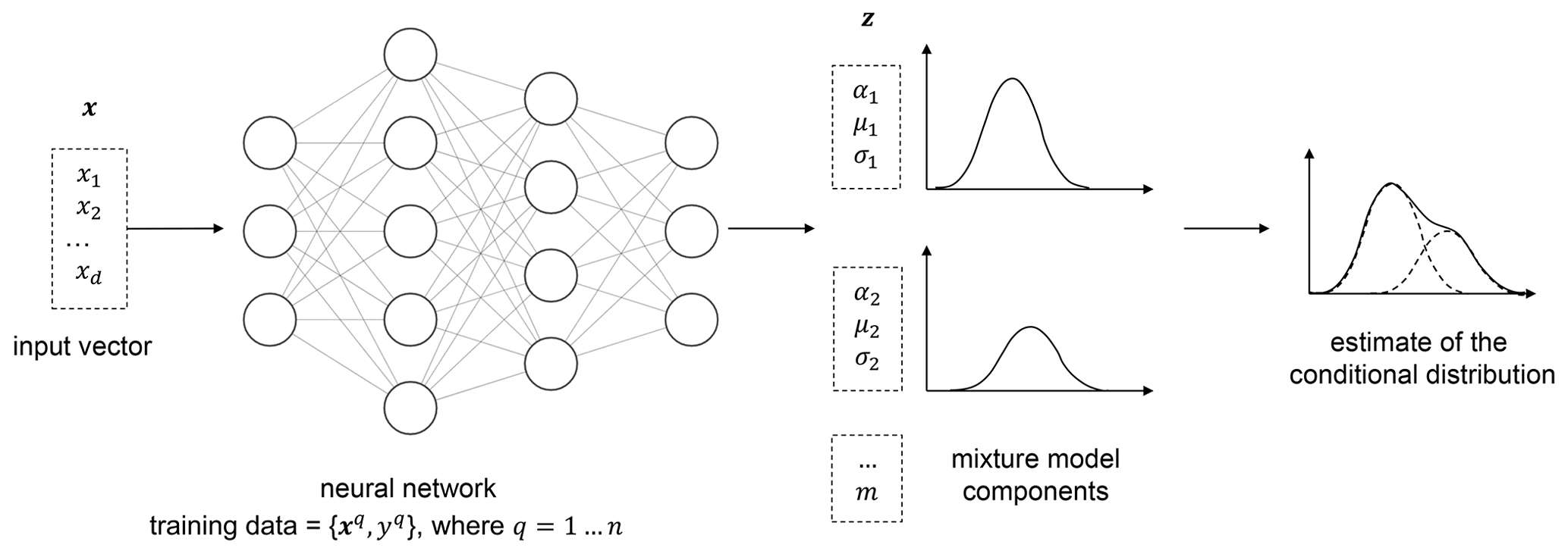
A mixture density network is a probabilistic regression method that combines Gaussian mixture models with artificial neural networks (Bishop, 1994). The conditional distribution of the target is represented by a mixture of Gaussian distributions,

$$\begin{array}{}\text{(9)}& p(y\mid \mathit{x})=\sum _{i=\mathrm{1}}^m{\mathit{\alpha }}_i\left(\mathit{x}\right)\mathcal{N}(y\mid {\mathit{\mu }}_i(\mathit{x}),{\mathit{\sigma }}_i^{\mathrm{2}}(\mathit{x}\left)\right),\end{array}$$

where α_i(x) are the weights or coefficients assigned to the ith mixture component and $\mathcal{N}(y\mid {\mathit{\mu }}_i(\mathit{x}),{\mathit{\sigma }}_i^{\mathrm{2}}(\mathit{x}\left)\right)$ is a Gaussian kernel representing the conditional density of the ith component of the target distribution, with parameters μ_i(x) and σ_i(x).

Instead of mapping the inflow features x to the load statistics y directly, the neural network is trained to predict the parameter vector, z∈ℝ consisting of α_j,μ_j, and σ_j for j=1…m.

Figure 2 Schematic representation of mixture density networks.

The mixing coefficients α_i(x) must sum up to exactly 1. A softmax function is used to handle this constraint,

$$\begin{array}{}\text{(10)}& {\mathit{\alpha }}_i={\displaystyle \frac{\exp z_i^{\mathit{\alpha }}}{{\sum }_{j=\mathrm{1}}^m\exp z_j^{\mathit{\alpha }}}},\end{array}$$

where $z_i^{\mathit{\alpha }}$ are the network outputs predicting the mixture coefficients. Similarly, positive values of the standard deviation are ensured by representing them as exponential functions of the corresponding network outputs, $z_i^{\mathit{\sigma }}$,

$$\begin{array}{}\text{(11)}& {\mathit{\sigma }}_i=\exp \left(z_i^{\mathit{\sigma }}\right).\end{array}$$

The likelihood ℒ of the dataset is given by

$$\begin{array}{}\text{(12)}& \mathcal{L}=\prod _{q=\mathrm{1}}^{n}p(y^q\mid {\mathit{x}}^q)p\left({\mathit{x}}^q\right).\end{array}$$

A very commonly used error function for probabilistic models is the negative log of the likelihood. From Eq. (9) and (12), the error can be written as

$$\begin{array}{}\text{(13)}& E^q=-\ln \left\{\sum _{i=\mathrm{1}}^m{\mathit{\alpha }}_i\left({\mathit{x}}^q\right)\mathcal{N}(y\mid {\mathit{\mu }}_i({\mathit{x}}^q),{\mathit{\sigma }}_i^{\mathrm{2}}({\mathit{x}}^q\left)\right)\right\},\end{array}$$

where p(x^q) is not included as it is constant with respect to the parameters or weights. The derivative of the error function is calculated at the output layer and is back-propagated to get its gradient with respect to the network weights. Finally, we have everything we need to minimize the error function using a gradient descent optimization. In this study, we use the Adam optimizer (Kingma and Ba, 2017) to perform stochastic gradient descent. A 10-fold cross-validation set over 600 samples is performed at every training.

The hidden layers in our network use the rectified linear unit (ReLU), defined as

$$\begin{array}{}\text{(14)}& \text{ReLU}\left(x\right)=\left\{\begin{array}{ll}x& \text{for }x>\mathrm{0}\\ \mathrm{0}& \text{for }x\le \mathrm{0}.\end{array}\right.\end{array}$$

The output layer of the network does not have an activation function; therefore, the outputs are just linear combinations of the inputs from the previous layer.

Minimizing the error function is an ill-posed problem as there is a conflict between learning the function that fits the data perfectly and remaining robust under varying sets of training data. As the network size grows, the function space increases, and the tendency of the neural network is to overfit. Among several ways to avoid overfitting (Montavon et al., 2012), in this study, we implemented a combination of early stopping (Yao et al., 2007) and L1 and L2 regularization (Ng, 2004).

2.2.1 Early stopping

The error function measured on the cross-validation dataset first decreases and then starts increasing as the network begins overfitting the training data. This can be avoided by applying an early stopping mechanism that stops training as the validation loss stops decreasing over a certain number of iterations. We experimented with a range of early stopping iterations and found 100 to be sufficient for the negative log likelihood on the validation dataset to converge but not overfit. That is, if the validation loss did not show any improvement after 100 iterations, we stopped training the model.

2.2.2 L1 and L2 regularization

L1 regularization penalizes the error function with the sum of the magnitude of the weights,

$$\begin{array}{}\text{(15)}& E_R^q=E^q+\mathit{\lambda }\sum \left|w_i\right|.\end{array}$$

It pushes the coefficients of uninformative features towards zero, effectively pruning the feature space (Tibshirani, 1996).

Weight decay or L2 regularization, on the other hand, penalizes the error function with a fraction of the squared magnitude of the weights,

$$\begin{array}{}\text{(16)}& E_R^q=E^q+\mathit{\lambda }\sum w_i^{\mathrm{2}}.\end{array}$$

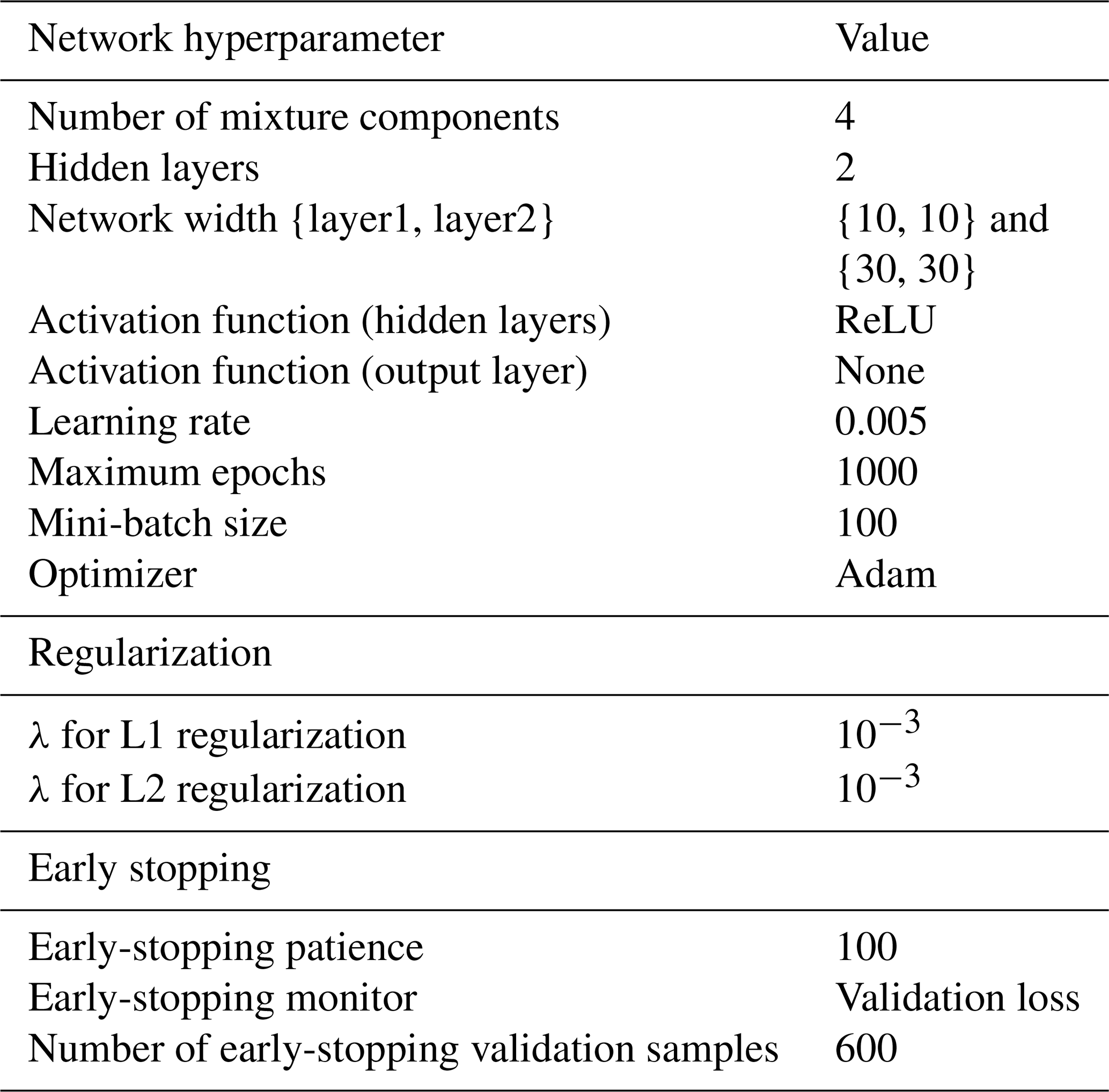
L2 regularization encourages the weights to be small. In both approaches, λ is the regularization parameter. It is a hyperparameter that controls the complexity of the model, and the optimal value can be chosen using a search algorithm. We found that heavy regularization with λ=0.1 for L1 and L2 regularization deteriorated the results by over-smoothing the conditional response. On the other hand, no L2 regularization also resulted in relatively smaller R² values for the standard deviation prediction, likely due to some degree of overfitting. On the basis of this hyperparameter study on one channel, we decided on a conservative λ value of 1e−3 for both L1 and L2 regularization.

The main hyperparameters used in this study to train the models to obtain the results in Sect. 4 are summarized in Table 1. In subsequent sections, we test the performance of the MDN model with two two-layer network architectures – the first with a width of 10 nodes per layer and the second with 30 nodes per layer. The features and targets are scaled with the standard scaler before training.

Table 1 Summary of the network hyperparameters.

3 Setup of the OpenFAST engineering model

3.1 OpenFAST modeling approach

The surrogate is modeled on the responses of an aero-hydro-servo-elastic code, OpenFAST, which is used as ground truth in this study. It is a state-of-the-art, multiphysics numerical tool for modeling wind turbines. It combines analytical and empirical formulations with conservative assumptions to simplify the code and limit the computational cost. It can model environmental conditions like stochastic waves, currents, and a frozen wind turbulence field with randomized coherent turbulent structures superimposed on the random, homogeneous, background turbulence.

OpenFAST is used for setting up a numerical model of the real-world environment and system dynamics to produce the training data for the surrogate. All simulations are performed on the IEA 10 MW (Bortolotti et al., 2019) offshore reference wind turbine. TurbSim (Jonkman and Buhl, 2007) simulations for inflow turbulence generation are performed with the Kaimal turbulence spectrum(Kaimal et al., 1972), a grid resolution of 40 points in a 1.16 D×1.16 D domain, with D being the rotor diameter. The spatial coherence is dictated by the IEC coherence function in the streamwise direction and no coherence in the plane orthogonal to the streamwise direction. The gradient Richardson number is set to 0. The total simulation duration is 900 s, out of which the first 300 s is discarded to exclude the initial transient. Based on the literature stated in Sect. 1.1, 10 min simulations on their own are insufficient for fatigue load estimations. However, the statistical variations in loads that one would expect over longer periods or multiple seed repetitions can be potentially inferred indirectly via probabilistic surrogates based on the variation in the quantities of interest at neighboring training samples. Therefore, 10 min statistics are sufficient for a complete description of the load response as long as unique turbulence and wave seeds are used for each training simulation.

The loads are calculated with the ElastoDyn module in OpenFAST, which uses the Euler–Bernoulli beam theory to calculate the bending moments by assuming the structure to be straight and isotropic. The ServoDyn module is used to control the wind turbine. The controller settings differ from the DTU Wind Energy controller used in the HAWC2 simulations of the IEA 10 MW reference document (Bortolotti et al., 2019). The main difference appears at low wind speeds, where the rotor rpm is not restricted to 6, and the collective blade pitch is zero until the rated wind speed. The OpenFAST simulation output with these controller settings at low wind speeds may interfere with the tower's natural frequencies; however, modification of the controller is beyond the scope of this study. The simulations are performed with single precision to limit file size and simulation times without any significant impact on the accuracy of the loads.

The implementation of the IEA 10 MW reference wind turbine (IEA-10MW-RWT) in OpenFAST is relatively new (Bortolotti et al., 2019). As such, there continue to be constant updates to the public model based on user feedback. This study uses the IEA-10MW-RWT as ground truth for the surrogate modeling study. For that purpose, it need not be perfectly accurate but representative of the expected load response class. The machine learning methodology is expected to be easily transferable to different wind turbine types.

3.2 Definition and sampling of the input features

The IEA-10MW-RWT is designed for offshore conditions. However, in this study, we simulate it on both onshore (CASE-ONSHORE) and offshore (CASE-OFFSHORE) sites to be able to evaluate the additional training requirements in the offshore case against an onshore reference.

3.2.1 CASE-ONSHORE

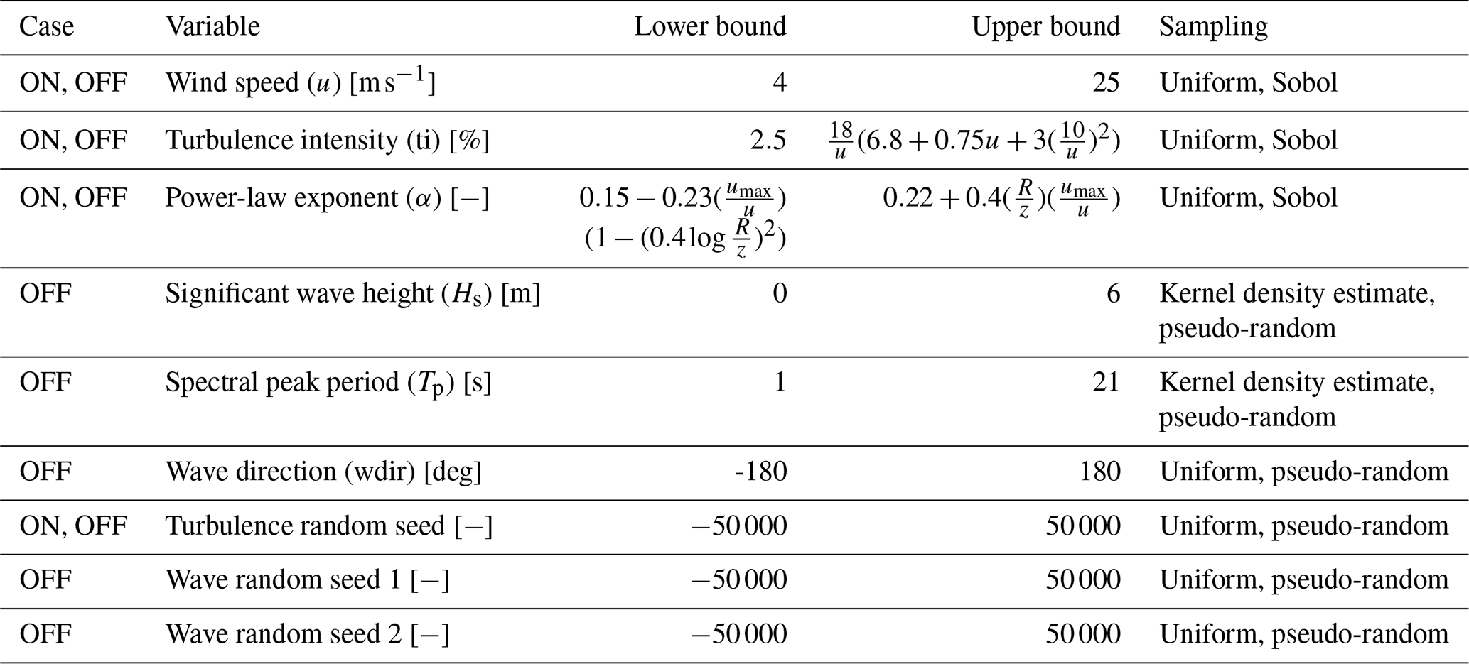
Aero-servo-elastic. The wind turbine is subjected only to aerodynamic loading. Wind speed, power-law exponent, and turbulence intensity are selected as the input parameters for the aerodynamic simulations as they have been shown to have the highest impact on the load response in previous studies (Dimitrov et al., 2018). The variable bounds are also the same as the ones defined in Dimitrov et al. (2018), listed in Table 2. The power-law exponent and turbulence intensity are functions of the wind speed. R and z are the rotor radius and the hub height, respectively. The samples are drawn from a three-dimensional Sobol sequence (Sobol, 1967) to ensure an even spread of points in the sample space. The random seed for turbulence generation is not included as a training variable. Each sample is therefore associated with a unique random seed; there are no repetitions.

Figure 3 Pair plot of the input features for CASE-OFFSHORE showing the training samples along with the test datasets. The marginal distributions are shown along the diagonal for the training dataset.

Table 2 List of input variables and the corresponding variable bounds for CASE-ONSHORE (ON) and CASE-OFFSHORE (OFF).

3.2.2 CASE-OFFSHORE

Aero-servo-hydro-elastic. The offshore wind turbine is placed on a monopile foundation at 30 m water depth and is subject to both aerodynamic and hydrodynamic loading. Along with the aerodynamic parameters of CASE-ONSHORE, there are additional wave parameters in this case as listed in Table 2. For designing load surrogates suitable for multiple sites, ideally the H_s–T_p diagrams from several sites should be combined to define conservative ranges for the two variables. In this study, as an example, we sample the values from a joint H_s–T_p kernel from a representative distribution. Additionally, the minimum and maximum range of H_s may also be defined as a function of wind speed in order to sample from the joint u–H_s–T_p distribution. The first-order waves are modeled using the JONSWAP spectrum in HydroDyn. The values of the aerodynamic variables are the same as in CASE-ONSHORE. In particular, the TurbSim solution files are therefore shared between CASE-ONSHORE and CASE-OFFSHORE. Similar to CASE-ONSHORE, the wave and turbulence seeds are not included in training the model. Each sample is therefore associated with a unique set of random seeds; there are no repetitions.

3.3 Responses

In this paper, we model the 10 min load statistics at the tower top and tower bottom in the fore–aft direction and at the blade root in the edgewise and flapwise directions. The statistics include the moment signal's 10 min standard deviation and DEL^ST. The modeled load channels are listed with their notation in Table 3. The model weights for each channel are calibrated separately.

Table 3 List of response channels modeled by the data-driven surrogate models.

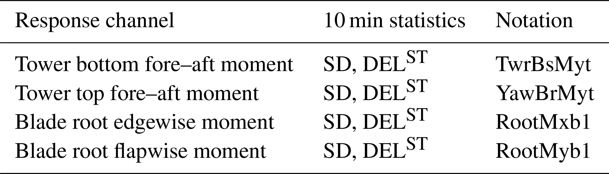
Since the direction of the incoming flow is always aligned with the rotor, the fore–aft direction at the tower base is defined in the local coordinate system of the inflow wind. The tower bottom loads must be projected appropriately in the global coordinate system of the wind turbine before integrating to calculate the lifetime fatigue damage in the global coordinate system. In this study, we only calculate the short-term damage in the local coordinate system. The 10 min fatigue is calculated using DEL^ST. DEL^ST converts the irregular load time series to a constant amplitude and frequency signal that produces an equivalent amount of fatigue damage loads. The rainflow-counting (Matsuishi and Endo, 1968) algorithm is used to obtain the load ranges S_i and the number of load cycles n_i needed to calculate the DEL^ST as

$$\begin{array}{}\text{(17)}& {\mathrm{DEL}}^{\mathrm{ST}}:={\left({\displaystyle \frac{n_i{S}_i^m}{n_{\mathrm{ref}}}}\right)}^{\mathrm{1}/m},\end{array}$$

where n_ref is 600 for 1 Hz DELs over 10 min. m is the Wöhler coefficient with values of 3.5 for the tower, 10 for blade flapwise, and 8 for blade edgewise moments.

3.4 Test datasets

The prediction accuracy of the conditional pdf by MDNs is tested on two independently sampled test datasets that have not been used in the training procedure, referred to as TEST1 and TEST2.

TEST1 consists of 50 pseudo-randomly selected points spanning the entire sampling domain, with parameter bounds the same as in Table 2. At each test point, engineering simulations with OpenFAST are repeated 300 times to get a reference pdf by keeping the input features constant but changing the turbulence and wave random seeds, resulting in a total of 15 000 TurbSim and OpenFAST simulations. In TEST2, we alter only the wind speed and turbulence intensity, keeping the other inflow parameters constant. TEST2 consists of 24 cases, each similarly repeated with 300 turbulence and wave seeds. The purpose of building a separate TEST2 dataset was to be able to visualize the performance of the model through 2-D heat maps in addition to analyzing the integrated quantities derived from TEST1. The values of the parameters are listed in Table 4.

Table 4 Variables and their corresponding values in the TEST2 dataset. Δ indicates the discretization step.

The test and training points for CASE-OFFSHORE are shown in Fig. 3. The marginal distributions are shown for the training dataset. The test points for CASE-ONSHORE are identical but only for the turbulence inflow features, namely, u, ti, and α.

Figure 4 shows, as an example, the 10 min average tower bottom fore–aft moment as a function of wind speed, along with the conditional distributions at two wind speeds from the TEST1 dataset. The surrogate models aim to predict this kind of conditional variation in the loads due to the stochastic inflow without the need for seed repetitions during training.

Figure 4 The left plot (a) shows the 10 min average tower bottom fore–aft moment as a function of wind speed. The samples belong to the training database of CASE-OFFSHORE. On the right (b–c), two examples of reference histograms generated using 300 turbulence seed repetitions in OpenFAST at wind speeds of 9.38 and 22.7 m s⁻¹ are shown from the TEST1 dataset.

3.5 Accuracy metric

The qualitative assessment of the performance of the surrogate model is based on two criteria: the coefficient of determination and the Wasserstein distance, as further described hereafter.

3.5.1 Coefficient of determination R²

The coefficient of determination, also known as the R², is a common measure of the goodness of fit of a model. It is defined as

$$\begin{array}{}\text{(18)}& R^{\mathrm{2}}=\mathrm{1}-{\displaystyle \frac{\sum (y_i-{\widehat{y}}_i)}{\sum (y_i-\overline{y})}},\end{array}$$

where $\widehat{y_i}$ is the predicted output, y_i is the observed value, and $\overline{y}$ is the mean of the observed values. R² is interpreted as the linear correlation between the predicted and observed values of the output vector. To assess the accuracy of the predicted conditional distribution of the response compared to the OpenFAST reference (Fig. 4), we calculate the R² value for the conditional pdf's mean, standard deviation, and 0.05 and 0.95 quantiles. These four quantities are derived empirically by obtaining 5000 samples from the surrogate-predicted conditional distribution and 300 turbulence seed repetitions per test case.

3.5.2 Wasserstein distance

The Wasserstein metric is a distance function to compare the difference between the pdfs of any two random variables. It is symmetric, non-negative, and satisfies the triangle inequality, making it a proper distance metric. In the case of 1-D distributions, the Wasserstein-2 distance between a reference empirical measure Y and predicted measure $\widehat{Y}$ is defined as (Villani, 2009; Peyré and Cuturi, 2019; Ramdas et al., 2015)

$$\begin{array}{}\text{(19)}& W_{\mathrm{2}}(Y,\widehat{Y})={\left(\underset{\mathrm{0}}{\overset{\mathrm{1}}{\int }}\left|F^{-\mathrm{1}}\right(t)-G^{-\mathrm{1}}(t){|}^{\mathrm{2}}\mathrm{d}t\right)}^{\mathrm{1}/\mathrm{2}},\end{array}$$

where F⁻¹ and G⁻¹ are the quantile functions of Y and $\widehat{Y}$, respectively. The individual quantile functions are obtained from the samples of the empirical distributions and then integrated. In this paper, we calculate the Wasserstein distance between the conditional distribution predicted for each sample ($\widehat{Y}$) and the conditional distribution obtained as a reference through seed repetitions in OpenFAST (Y). $\widehat{Y}$ consists of 5000 samples, and Y is obtained from 300 turbulence seed repetitions. The distance metric is normalized by the standard deviation of the reference conditional distribution, Y. Therefore, a value of $\frac{W_{\mathrm{2}}}{\mathit{\sigma }\left(Y\right)}=\mathrm{1}$ is the distance between a distribution with mean μ(Y), scale σ(Y), and a degenerate distribution with the same mean. We calculate the global performance of the model by averaging the normalized Wasserstein distance over N_test test samples as

$$\begin{array}{}\text{(20)}& d_{W\mathrm{2}}={\mathbb{E}}_{N_{\mathrm{test}}}\left({\displaystyle \frac{W_{\mathrm{2}}}{\mathit{\sigma }\left(Y\right)}}\right).\end{array}$$

Figure 5 CASE-ONSHORE: panels showing the change in the normalized 2-Wasserstein distance, R² value of the mean, 0.05 quantile, and 0.95 quantile of the predicted pdf as a function of the training samples. The study is performed on the tower base fore–aft moment standard deviation (TwrBsMyt SD). The numbers in the square bracket [x,x] denote the widths of the first and second layer of the two-layer neural networks.

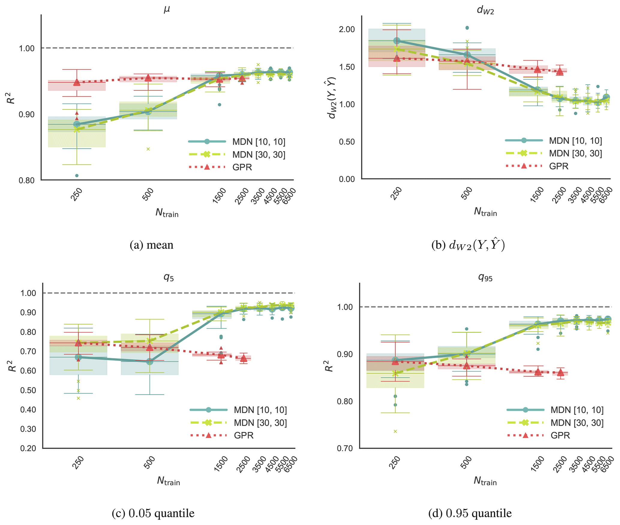
Figure 6 CASE-OFFSHORE: panels showing the change in the normalized 2-Wasserstein distance, R² value of the mean, 0.05 quantile, and 0.95 quantile of the predicted pdf as a function of the training samples. The study is performed on the tower base fore–aft moment standard deviation (TwrBsMyt SD). The numbers in the square bracket [x,x] denote the widths of the first and second layer of the two-layer neural networks.

4 Results and discussion

In this section, we assess how well the surrogate models predict the conditional load distribution on the TEST1 and TEST2 datasets mentioned in Sect. 3.4. The first part focuses on convergence studies, specifically the impact of training data size on the prediction of the average 10 min standard deviation of the tower bottom fore–aft moment. The goal is to measure how the accuracy of the predictions varies based on the hyperparameters and initialization of the optimization algorithm. Once the network architecture and training sample size are fixed, we do a rigorous analysis of the model's performance in Sect. 4.2.

4.1 Convergence

Generally speaking, more data translate to better accuracy. However, an increase in data after a certain point gives diminishing returns in accuracy. Given the computational cost of generating the training database, we want to ensure a good model fit with as few training data as possible.

In this section, we look at the convergence of the model with respect to the number of training samples in two two-layer networks with 10 ([10,10]) and 30 ([30,30]) units in each layer. Two different networks are chosen to comment on the robustness of the approach with respect to the network architecture. The convergence study is performed both on CASE-ONSHORE in Fig. 5 and on CASE-OFFSHORE in Fig. 6. The boxes in Figs. 5 and 6 extend between the first (Q1) and third (Q3) quartile of the data, and the horizontal line across the box indicates the median. The difference between Q1 and Q3 defines the interquartile range (IQR). The upper whisker extends to the largest data values that are within 1.5 IQR above Q3. The lower whisker, similarly, extends to the lowest data point within 1.5 IQR below Q1. Outliers are visible as dots beyond the whisker boundaries.

The network is trained on the tower bottom fore–aft moment standard deviation (TwrBsMyt [kN m] SD). In principle, the convergence study could be performed on any or all of the load channels mentioned in Sect. 3.3. However, TwrBsMyt [kN m] SD was chosen because it is found to have relatively the highest average d_W2 value amongst all channels. Models are data-dependent, and each channel would ideally need a separate sensitivity study in terms of the number of training samples needed for convergence, the model architecture, and the model hyperparameters. However, for practical purposes, we assume that if a model can perform well on the channel with the poorest metrics, then it should also perform well, if not optimally, on the other load channels with the same network architecture. Care is taken to prevent overfitting by comparing the evolution of the negative log likelihood on the training and test datasets during training. At every N_train, the model training is repeated on 25 uniquely sampled subsets of the data with 10-fold cross-validation. The plots in Fig. 6 show the convergence of the model in terms of predicting the normalized 2-Wasserstein distance and statistics, including the response pdf's mean, 0.05 quantile, and 0.95 quantile. The metrics are averaged over the validation dataset formed by combining TEST1 and TEST2.

Figures 5 and 6 also show the Gaussian process regression predictions with 25 repetitions. We expect GPR to only predict the right estimate of the mean of the response. Since it is based on Bayesian inference, which is very different from the back-propagation mechanism used in MDNs, it can infer the response estimate with a much smaller training dataset. The GPR model is not trained on datasets larger than 2500 samples because it scales poorly and the training expense grows exponentially as mentioned in Sect. 2.1.

Figure 7 Training and validation losses for the [10, 10] MDN with 500 (a) and 4500 (b) training samples, CASE-ONSHORE.

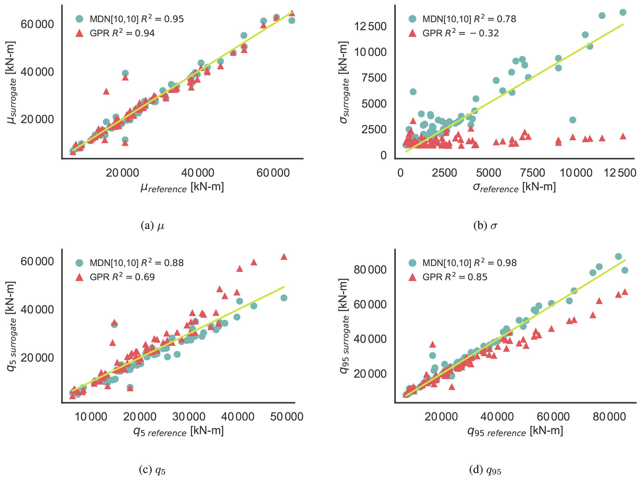
Figure 8 CASE-OFFSHORE: prediction of the statistics of the response pdf of the 10 min damage equivalent loads for the tower base fore–aft moment.

In both CASE-ONSHORE and CASE-OFFSHORE, the difference between the predictions of the two MDN architectures [10,10] and [30,30] is negligible for μ, q₅ and q₉₅. An improvement of roughly 15 % in terms of d_W2 is seen in CASE-ONSHORE, whereas a negligible difference is observed in CASE-OFFSHORE. As we do not have an infinite pool of data, the uncertainty bounds concerning the choice of the training samples are progressively reduced as we approach the total available training samples. At smaller N_train values, the uncertainty is also driven by the missing information in the training data and the choice of the initial conditions used by the stochastic gradient descent optimizer. Significantly better GPR estimates of the response mean for less than 1500 training samples can be attributed to the Bayesian formulation. Beyond that point, however, MDNs and GPR are comparable, with R²>0.99 in CASE-ONSHORE and R²>0.95 in CASE-OFFSHORE. MDN shows significantly better predictions of all other quantities.

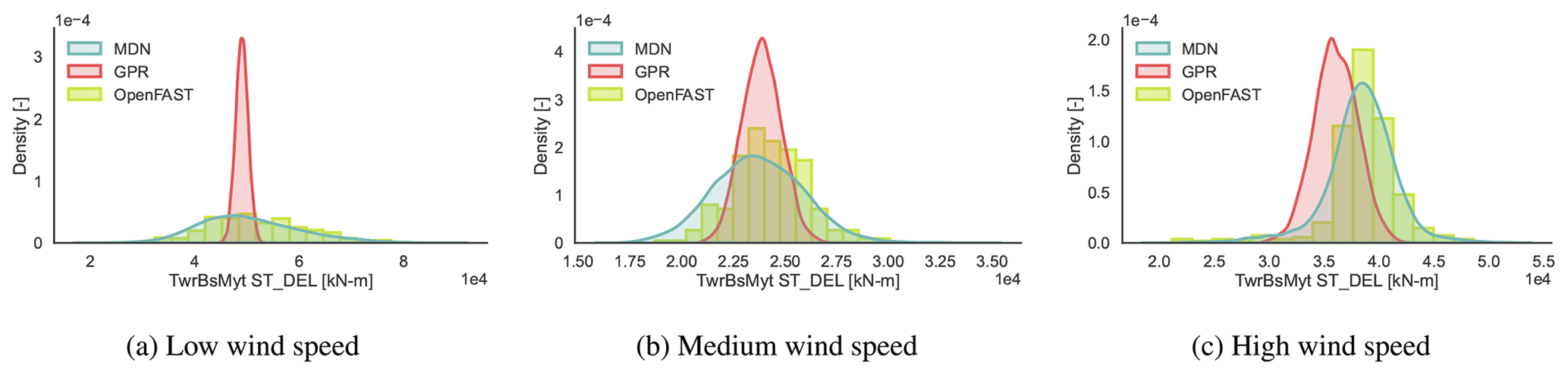
Figure 9 CASE-OFFSHORE: predicted and reference (OpenFAST) conditional pdf for the tower base fore–aft moment DEL^ST.

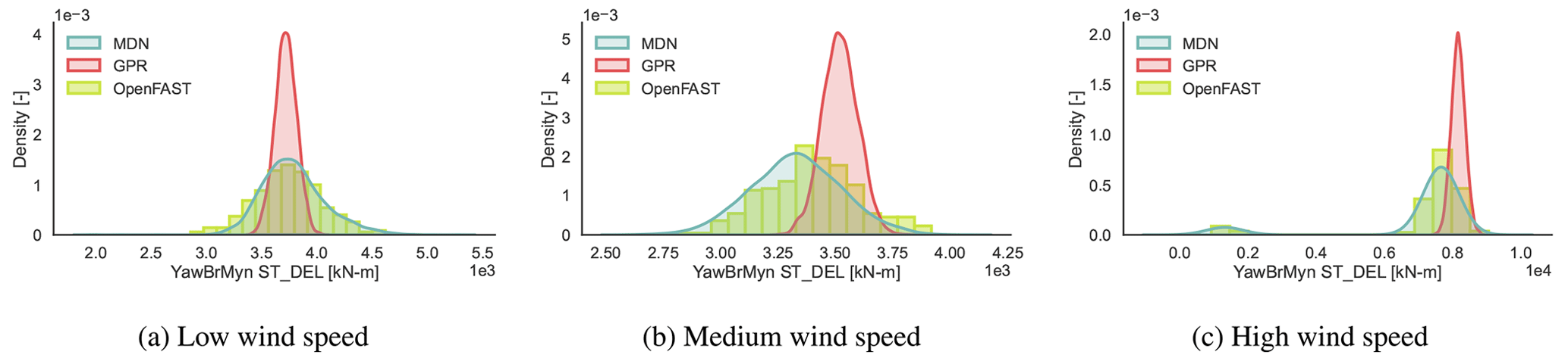
Figure 10 CASE-OFFSHORE: predicted and reference (OpenFAST) conditional pdf for the tower top fore–aft moment DEL^ST.

Table 5 Comparison of the prediction of the statistical properties of the response pdf for the tower base fore–aft loads. The table lists the R² values observed for the statistics of the tower bottom fore–aft load channel for the onshore and offshore test cases.

The estimates of the tails of the pdf, quantified by the lower 0.05 quantile, are well captured by MDN in both onshore and offshore case studies. Overall, the model's accuracy in terms of the statistical quantities is approximately 5 % better in CASE-ONSHORE for the same number of training points. However, d_W2 is 50 % smaller in CASE-ONSHORE than in CASE-OFFSHORE, signifying, overall, a much better inference of the latent pdf in the onshore conditions than offshore. This is expected, as the larger the degrees of freedom, the larger the space between the neighboring points. The goodness of fit of the model in terms of d_W2 depends on the rate of change of the statistics of the underlying distributions. The gradient of the standard deviation, in particular, is much harder to infer from a cloud of points than the gradient of the mean. The convergence plots for CASE-OFFSHORE could indicate either that this is the best estimate of d_W2 achievable, given the information the model has, or that the number of samples needed to capture the variation in the standard deviation are much larger than the maximum training sample size that we tested.

Figure 7 shows the training and validation losses plotted against the number of epochs for CASE-ONSHORE. MDN overfits the data at N_train=500 because as the training loss decreases, the validation loss increases, indicating that the model cannot handle previously unseen data. Figure 7b is well fitted as the training and validation losses decrease at the same rate. The plot also shows the auto-stop algorithm at work, which halts training after 100 epochs of approximately zero-gradient loss to avoid overfitting.

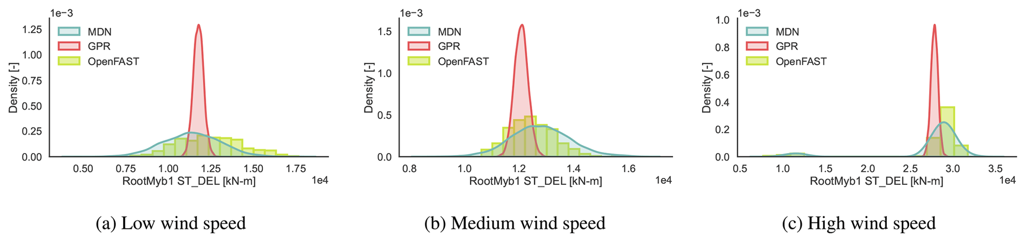
Figure 11 CASE-OFFSHORE: predicted and reference (OpenFAST) conditional pdf for the blade root flapwise moment DEL^ST.

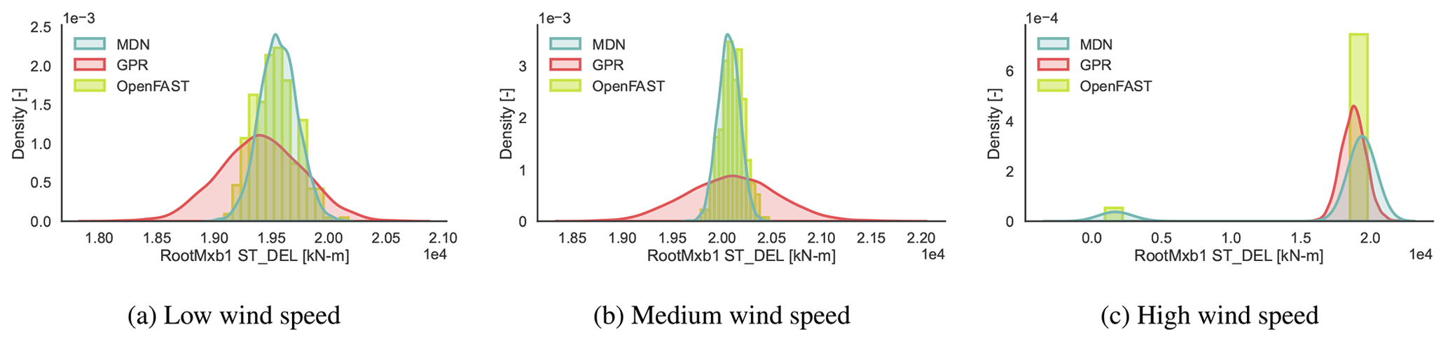
Figure 12 CASE-OFFSHORE: predicted and reference (OpenFAST) conditional pdf for the blade root edgewise moment DEL^ST.

Table 6 CASE-OFFSHORE: comparison of the channel-wise prediction of the R² values of the mean and standard deviation using MDN and GPR.

For the remainder of this study, we will use a two-layer MDN with 10 activation units in each layer trained on 4500 samples. It offers a good balance between training time, model complexity, and accuracy. For GPR, a training set of 500 samples will be used as it is found to be sufficiently accurate.

4.2 Load prediction

In this section, we evaluate the prediction of the 10 min damage equivalent loads on the wind turbine for CASE-ONSHORE and CASE-OFFSHORE. Table 5 summarizes the predictions of various statistical properties of the response pdf for both cases in terms of the R² values. R² values reflect the proportion of variance in the output that is predictable from the surrogate models. The absolute magnitude of R² is sensitive to the optimization initialization, the choice of the test samples, and the choice of the training subset as seen in Fig. 6. It is, therefore, important to note that the absolute R² values do not carry much objective meaning on their own. They are only used here for comparing the performance of models relative to one another. Figure 8 shows the corresponding plots for CASE-OFFSHORE.

Overall, MDN performs better than GPR across all the metrics listed in Table 5 for CASE-ONSHORE and CASE-OFFSHORE. The conditional average, μ, is well estimated by both models. The standard deviation, σ, is constant in the case of the GPR model, as it is a homoscedastic formulation. This, as expected, is reflected through the negative values of R², indicating no correlation between the σ estimated from the GPR model and the reference σ values. The minor variations in Fig. 8b in σ_surrogate can be attributed to a combination of model uncertainty and Monte Carlo sampling. Estimates of the standard deviation by MDN are excellent in CASE-ONSHORE, but the performance drops in CASE-OFFSHORE. However, the results are encouraging compared to GPR and show that MDN can handle heteroscedastic datasets. The 0.05 and 0.95 quantiles, which are essential for design considerations, are exceptionally well predicted by MDN. In Fig. 8c and d, GPR shows a bias in the quantile estimate, increasing with the quantity's magnitude, which can be directly ascribed to the underestimation of the standard deviation of the response.

The R² values show that the model fit for CASE-ONSHORE is relatively better than for CASE-OFFSHORE. As noted in the previous section, it appears to be much easier to train a case with only aerodynamic features for the same number of training samples and network architecture.

Table 6 compares the R² values calculated for DEL^ST of various load channels on CASE-OFFSHORE by MDN and GPR. Both MDN and GPR show relatively high accuracy in estimating the mean DEL^ST for the tower channels. Specifically, the tower bottom and top fore–aft channels have R² values above 0.94 for MDN, indicating strong predictive performance. However, a notable discrepancy is observed in the GPR predictions for the mean blade root edgewise DEL^ST. We noted that the GPR predictions were especially sensitive to the value of the initial length-scale vector used for training this channel. Further investigations show that up to 18 m s⁻¹, the GPR is able to correctly estimate the mean blade root edgewise DEL^ST. However, between 18 and 20 m s⁻¹, the values are overestimated, and above 20 m s⁻¹, they are underpredicted, leading to a smaller R². This behavior could be attributed to large gradients in the response surface and insufficient data samples at high wind speeds. The conditional response at high wind speed in Fig. 12c also shows the potential for this bias due to the presence of a few data samples with very low fatigue values at high wind speed and high turbulence intensity, as the wind turbine switches to the idling regime in some cases.

Figure 13 Normalized 2-Wasserstein distance computed on the CASE-OFFSHORE validation dataset for the MDN model. The performance is plotted on a turbulence intensity and wind speed grid.

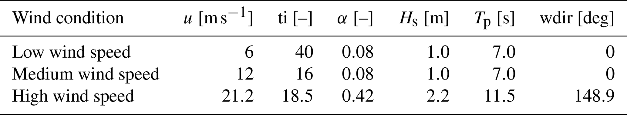
The DEL^ST for the tower base fore–aft moment (Fig. 9), tower top fore–aft moment (Fig. 10), blade root flapwise moment (Fig. 11), and blade root edgewise moment (Fig. 12) is plotted at three operational conditions falling in low-, medium-, and high-wind-speed blocks. The values of the input features are noted in Table 7.

Table 7 Values of the input features for the pdfs in Figs. 9, 10, 11, and 12.

Clearly, the responses are not always normally distributed. The variance of the response is not constant across wind speeds. Near the cut-out wind speed, we also notice a multi-modal response, as the wind turbine switches between idling and power production, depending on the local variations in the inflow wind patterns. Here, MDN is shown to leverage the flexibility of learning complex noise patterns to then approximate the full picture of the response that deterministic models could otherwise miss.

In Fig. 13, d_W2 is plotted on the TEST2 dataset. We notice that there are certain test samples where neither MDN nor GPR is successful in inferring the underlying function. From the figure, it appears that the model is consistently unable to detect the correct patterns at very low turbulence intensities across different wind speeds and load channels. Figure 14 shows the conditional pdf plots for the tower base fore–aft DEL^ST at 4 % turbulence intensity, corresponding to the high-d_W2 regions in the heatmap in Fig. 13a. The figures correspond to wind speeds of 12, 15, and 18 m s⁻¹. The other input parameters are fixed at the values indicated in Table 4. Both GPR and MDN overpredict the standard deviation of the response in this regime, resulting in the relatively high d_W2 values. Since we do not see a similar decline in performance at the tower top, fatigue driven mainly by hydrodynamic load variation at low turbulence intensities may be difficult for the model to capture. Increased training sample density in this region could benefit performance, but this has yet to be investigated. Application-wise, these regions are not the most critical, as fatigue is primarily driven by larger turbulent disturbances.

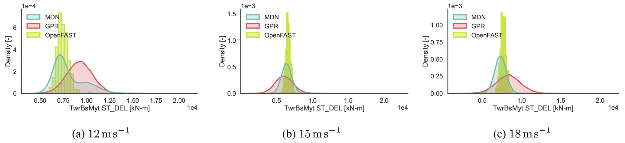
Figure 14 CASE-OFFSHORE: predicted and reference (OpenFAST) conditional pdf for the tower base fore–aft DEL^ST at low turbulence intensity (4 %) values at wind speed of 12, 15, and 18 m s⁻¹.

5 Conclusions

This paper presents a novel probabilistic approach based on mixture density networks to make efficient and flexible load surrogates for offshore siting. The data-driven surrogate uses aero-servo-hydro-elastic OpenFAST simulations of the 10 MW reference wind turbine for training. We compare the performance of MDN to the widely used Gaussian process regression model and show an improvement in the estimation of the load uncertainty associated with the stochastic representation of inflow turbulence and waves.

The surrogate is trained on a wind turbine subject to aerodynamic (CASE-ONSHORE) and aero-hydrodynamic (CASE-OFFSHORE) loading with the intent of comparing the difficulty in designing load surrogates for the two cases. The reference conditional pdfs for validating the models' performance are produced using 300 random seeds at each of the test operating conditions. A convergence study is performed to assess the accuracy of the surrogate as a function of the number of training samples. Two different MDN architectures and the standard Gaussian process regression are evaluated. It is shown that the surrogate is more accurate for the same number of training samples in CASE-ONSHORE (three features) as opposed to CASE-OFFSHORE (six features), based on the 2-Wasserstein distance between the predicted and the reference conditional pdf of the response. A minimum of 2500 samples are required by MDN to surpass an R² value of 0.95 for the prediction of the mean and quantiles in CASE-OFFSHORE. The GPR model is shown to be more accurate in predicting the mean of the response even with a small dataset of 250 samples. In applications where the surrogate must be trained frequently on new cases, say, for new geometries of the blade or tower, GPR provides a big advantage in limiting the computational cost of training. Beyond 1500 samples, MDN predictions are consistently better. The quantiles are well captured by MDN in both cases.

The conditional pdfs from the validation dataset are evaluated for low-, medium-, and high-wind-speed cases to demonstrate the ability of MDN to capture heteroscedastic, multi-modal responses with high accuracy, even with limited training data. We note a poor performance of the MDN model at low-turbulence-intensity conditions across all load channels, indicating either the need for a higher sampling rate in those regions in the training dataset or the presence of a sharp gradient in the response surface that the model could not appropriately capture.

This work shows promising results for using MDN and GPR as surrogates in site assessment of onshore and offshore wind turbines. The MDN model probabilistic modeling of the loads, although shown to have a slight improvement in the prediction of the expectation of the response compared to the state-of-the-art Gaussian process regression, can capture the variances and quantiles of the response far better. With the added benefit of not needing seed repetitions prior to training, we show that both approaches cut down significantly on the computational cost associated with generating the training database without compromising on the accuracy of prediction. Work is currently in progress to determine how the information on the uncertainty in the short-term load response can be propagated to the lifetime loads to help inform engineering decisions.

Appendix A: Machine learning framework

Figure A1 shows the basic framework used for model calibration and load estimation. All data generated from OpenFAST are included in the training base without any repetition or pre-filtering step involved.

Figure A1 Schematic of the machine learning framework.