On the robustness of a blade-load-based wind speed estimator to dynamic pitch control strategies

In the context of wind turbine pitch control for load alleviation or active wake mixing, it is relevant to provide the time- and space-varying wind conditions as an input to the controller. Apart from classical wind measurement techniques, blade-load-based estimators can also be used to sense the incoming wind. These consider blades to be sensors of the flow and rely on having access to the operating parameters and measuring the blade loads. In this paper, we wish to verify how robust such estimators are to the control strategy active on the turbine, as it impacts both operating parameters and loads. We use an extended Kalman filter (EKF) to estimate the incoming wind conditions based on the blade bending moments. The internal model in the EKF relies on the blade element momentum (BEM) theory in which we propose accounting for delays between pitch action and blade loads by including dynamic effects. Using large-eddy simulations (LESs) to test the estimator, we show that accounting for the dynamic effects in the BEM formulation is needed to maintain the estimator accuracy when dynamic wake mixing control is active.

1 Introduction

With their 2030 Agenda for Sustainable Development, the United Nations (2015) set 17 goals to ensure the sustainable development of our planet. Sustainable Development Goal number 7 aims at ensuring access to affordable, reliable, sustainable, and modern energy for all. In that perspective, reducing the levelized cost of energy (LCoE) coming from wind is essential. Two factors contributing to this effort are considered here: increasing wind farm power capture and reducing the occurrence of turbine failures. Wind turbine and wind farm flow control can contribute to these two objectives.

Individual pitch control (IPC) has shown its potential to reduce structural loads, from numerical studies (Bossanyi, 2003) to experimental demonstrations (Bossanyi et al., 2013). In the meantime, several wind farm flow control strategies have been considered to mitigate wake effects and maximize power production in wind farms. Static flow control was originally proposed, mostly wake redirection using yaw control (Fleming et al., 2014; Wagenaar et al., 2012). Dynamic flow control has also been investigated, mostly the pulse approach and the helix approach. The first one, the pulse approach, relies on collective pitch control (CPC) to periodically vary the thrust force of the turbine at a frequency that is typically 1 order of magnitude smaller than the turbine rotation frequency (Yilmaz and Meyers, 2018; Munters and Meyers, 2018). The resulting changes in induction generate pulsating patterns in the wake, which help it destabilize faster. When it comes to the helix approach, IPC is used to generate sinusoidal variations of the tilt and yaw moments in quadrature phase (Frederik et al., 2020). As a consequence, the wake propagates downstream following the shape of a helix, and its recovery is enhanced (Korb et al., 2023). Both strategies come with additional loading and pitch-bearing activity (Frederik and van Wingerden, 2022; van Vondelen et al., 2023b).

Let us focus the remainder of this review on pitch-actuation-based control strategies, for which wind condition awareness is often very limited. In the case of load alleviation using IPC, some studies have proposed controllers including explicit information about the incoming wind, such as the rotor-effective wind speed measured by a lidar in Russell et al. (2024). Still, for most IPC controllers, the measurements used to determine the control actions are the blade loads (Bossanyi, 2003; Lu et al., 2015). When it comes to dynamic wake mixing, the pulse and helix strategies act in an open-loop manner. In previous experimental and numerical contributions (van der Hoek et al., 2024; Korb et al., 2023; Taschner et al., 2023), the pitch actuation frequency is fixed for a studied configuration. It is computed based on the mean infinite upstream wind speed to match a chosen Strouhal number.

Yet refined wind condition awareness could be essential to developing more efficient controllers (Meyers et al., 2022). When it comes to load alleviation, Selvam et al. (2009) showed that including a feedforward loop based on wind disturbance estimation in the IPC scheme further reduces structural loads. Russell et al. (2024) additionally demonstrated how lidar-assisted feedforward IPC was improving load alleviation results for turbines operating in freestream conditions. Coquelet et al. (2022) investigated the case of waked turbines and concluded that it created challenges, calling for new IPC schemes accounting for partial or total wake impingement. When it comes to wake mixing, the controllers act in a dynamic way. How the actuation is phased with respect to turbulent structures in the incoming flow therefore influences their efficiency in alleviating wake effects. Munters and Meyers (2018), for instance, showed, using an optimal control framework for dynamic induction control, that the vortex rings generated by the optimal controller coincide with bulges that are naturally present in the wake of the reference case. The turbine actuation thus phases itself with the incoming turbulent flow structures. The studies of van Vondelen et al. (2023a) and Korb et al. (2023) also showed, in the context of a line of three turbines, that the pitch phase offset between the first and the second turbine influences the power leveraged for the third turbine.

Though these examples highlight the potential of wind condition awareness in the context of wind turbine and wind farm flow control, they still lack practical implementation due to sensing limitations. Anemometers have been present on nacelles for many years (Smith et al., 2002). Yet, they only provide information on the wind at the measurement point, making turbines unaware of wake impingement, shear, or turbulent gusts. Their measurements additionally suffer from a number of disturbances, resulting in unreliable measurements (Bottasso et al., 2018). Consequently, nacelle-mounted lidars have received growing attention, as they provide solutions to these limitations. They offer remote sensing and are able to provide a great characterization of the incoming flow. Most importantly, lidars are able to measure the incoming flow further upstream from the turbine, hence allowing the controller to prepare for future flow variations. For this reason, lidars are good candidates for feedforward control approaches (Letizia et al., 2023; Scholbrock et al., 2016). They are not a standard yet for modern turbines, likely due to their cost, complexity of installation, or need for synchronization with the SCADA (supervisory control and data acquisition) system. However, their industrial use has been reported (Raach, 2021) and is likely to be generalized in the future.

Alternative methods to characterize the inflow have also been investigated. They are based on the principle that any change in the wind is reflected in the load response of the rotor and that load sensors are now typically available for modern turbines (Cooperman and Martinez, 2015; Bottasso et al., 2018). This is referred to as the rotor-as-a-sensor approach, for which the structural response of the turbine is used to determine the wind conditions. Conversely to lidars, such approaches do not offer a preview of the future incoming wind, and the estimation is limited to the current wind conditions. Several contributions on the topic rely on estimators derived from Kalman filters. Simley and Pao (2016) present a linear Kalman-filter-based estimator for estimation of hub-height wind speed and wind shear components. Interestingly, the authors show that the estimator performances degrade when blade pitch actuation occurs due to the nonlinearities appearing in the turbine response. Bottasso et al. (2018) introduce an extended Kalman filter (EKF) formulation to estimate blade-effective wind speeds. These are then transformed into sector-effective wind speeds for wake detection application. In Bertelè et al. (2017), this approach is extended to the estimation of inflow misalignment and shear angles through the identification of the blade load harmonics. The EKF approach is also reported in Lejeune et al. (2022), where the sensing is used to infer flow information to a meandering-capturing wake model developed for operational wind farm flow prediction. In Brandetti et al. (2023), it is an unscented Kalman filter that is used for blade-effective wind speed estimation on vertical-axis wind turbines. Other types of estimators have also been reported, such as a subspace predictive repetitive estimator in Liu et al. (2021) and both a proportional integral notch estimator and a Coleman-based estimator in Liu et al. (2022).

This work investigates the ability of these blade-load-based estimators to infer the characteristics of the incoming wind when the turbine is operated with several advanced control strategies. Indeed, the underlying principle of load-alleviation IPC, the pulse approach, and the helix approach is to use pitch actuation to modify blade loads. We wonder whether a blade-load-based estimator can still be accurate in that context and therefore be used for closed-loop control applications. To answer this question, we deploy an EKF using the blade out-of-plane bending moments to estimate wind speed at both the rotor scale and more local scales, building upon the work of Bottasso et al. (2018). Kalman-filter-based estimators rely on an internal model of the turbine relating the measurements and the estimations. Linearized models cover only a small range of turbine operation and lead to inaccuracies out of that range (Simley and Pao, 2016; van Vondelen et al., 2023a), while nonlinear look-up tables (Bottasso et al., 2018; Liu et al., 2021) cannot account for dynamic effects between actuation and loads. Regarding the dynamic pitching context into which this paper falls, we propose the use of a dynamic BEM formulation, covering the whole range of operation of the turbine and accounting for potential delays between pitch actuation and blade loads. We demonstrate the performance of the estimator using large-eddy simulations (LESs). The simulated blade bending moments and turbine operating parameters are fed to the estimator, and the wind speed estimates are validated against the actual velocity field retrieved from the LES. We then verify the accuracy of the estimator in cases where pitch control strategies are active for load alleviation and for wake mixing.

The contributions are thus threefold.

1. Formulate a blade-load-based estimator using a BEM as the internal model in the EKF.

2. Include dynamics in the BEM to account for delays between pitch action and blade loads in the context of dynamic pitch control.

3. Verify the robustness of this estimator to load alleviation and wake mixing control strategies in LES.

The remainder of the paper is organized as follows. Section 2 introduces the EKF and the testing environment. The performances of the estimator on a single turbine immersed in turbulent wind are assessed in Sect. 3. The robustness of the blade-load-based estimator is evaluated for turbines using load alleviation and wake mixing control in Sect. 4. Eventually, conclusions are drawn alongside perspectives in Sect. 5.

2 Methodology

This section presents the structure of the blade-load-based estimator and briefly describes the LES environment in which it is tested.

2.1 Extended Kalman filter for wind speed estimation

The general procedure of the EKF theory is recalled before being applied to the estimation of blade-effective wind speeds. How the latter are then used to reconstruct several characteristics of the wind speed impinging on the rotor is then presented.

2.1.1 Extended Kalman filter

Consider the discrete-time state-space representation of a nonlinear system:

$$\begin{array}{}\text{(1)}& {\displaystyle }{\mathit{x}}_k=\mathit{f}\left({\mathit{x}}_{k-\mathrm{1}},{\mathit{u}}_{k-\mathrm{1}}\right)+{\mathit{w}}_{k-\mathrm{1}},\text{(2)}& {\displaystyle }{\mathit{y}}_k=\mathit{h}\left({\mathit{x}}_k,{\mathit{u}}_k\right)+{\mathit{v}}_k,\end{array}$$

with x_k the state vector at time instant k, y_k the output or measurement vector, and u_k the control input vector. $\mathit{f}\left({\mathit{x}}_{k-\mathrm{1}},{\mathit{u}}_{k-\mathrm{1}}\right)$ is the nonlinear state function and h(x_k,u_k) is the measurement function. w_k is the process noise vector and v_k is the measurement noise vector. In EKF theory, they are assumed to be zero-mean Gaussian white noise with covariance matrices Q and R, respectively (Chui and Chen, 2017).

The purpose of the EKF is to compute an estimate of the unknown states x based on the system model and input–output signals. It is an extension of the linear Kalman filter in the sense that it generalizes the formulation to nonlinear systems. To do so, it relies on the Jacobian matrices of the state and measurement functions for the prediction and correction step, respectively (Chui and Chen, 2017).

The prediction step at time k consists of computing the a priori error covariance estimate ${\mathbf{P}}_k^{-}$ and the a priori state estimate ${\widehat{\mathit{x}}}_k^{-}$ based on the previous estimates of the covariance matrix ${\mathbf{P}}_{k-\mathrm{1}}^{+}$ and the state ${\widehat{\mathit{x}}}_{k-\mathrm{1}}^{+}$, and the Jacobian matrix of the state function F_k−1. The computation is as follows.

$$\begin{array}{}\text{(3)}& {\displaystyle }{\mathbf{F}}_{k-\mathrm{1}}={\left.{\displaystyle \frac{\partial \mathit{f}}{\partial \mathit{x}}}\right|}_{{\widehat{\mathit{x}}}_{k-\mathrm{1}}^{+},{\mathit{u}}_{k-\mathrm{1}}}\text{(4)}& {\displaystyle }{\mathbf{P}}_k^{-}={\mathbf{F}}_{k-\mathrm{1}}{\mathbf{P}}_{k-\mathrm{1}}^{+}{\mathbf{F}}_{k-\mathrm{1}}^T+\mathit{Q}\text{(5)}& {\displaystyle }{\widehat{\mathit{x}}}_k^{-}=\mathit{f}\left({\widehat{\mathit{x}}}_{k-\mathrm{1}}^{+},{\mathit{u}}_{k-\mathrm{1}}\right)\end{array}$$

The correction step then makes use of the measurement z_k to compute the a posteriori state estimate ${\widehat{\mathit{x}}}_k^{+}$ and the a posteriori error covariance matrix ${\mathbf{P}}_k^{+}$ based on the Jacobian matrix of the measurement function H_k, the measurement residual ${\stackrel{\mathrm{̃}}{\mathit{y}}}_k$ and the Kalman gain K_k. The procedure is as follows.

$$\begin{array}{}\text{(6)}& {\displaystyle }{\mathbf{H}}_k={\left.{\displaystyle \frac{\partial \mathit{h}}{\partial \mathit{x}}}\right|}_{{\widehat{\mathit{x}}}_k^{-},{\mathit{u}}_k}\text{(7)}& {\displaystyle }{\mathbf{K}}_k={\mathbf{P}}_k^{-}{\mathbf{H}}_k^T{\left(\mathbf{R}+{\mathbf{H}}_k{\mathbf{P}}_k^{-}{\mathbf{H}}_k^T\right)}^{-\mathrm{1}}\text{(8)}& {\displaystyle }{\mathbf{P}}_k^{+}=\left(\mathbf{I}-{\mathbf{K}}_k{\mathbf{H}}_k\right){\mathbf{P}}_k^{-}\text{(9)}& {\displaystyle }{\stackrel{\mathrm{̃}}{\mathit{y}}}_k={\mathit{z}}_k-\mathit{h}\left({\widehat{\mathit{x}}}_k^{-},{\mathit{u}}_k\right)\text{(10)}& {\displaystyle }{\widehat{\mathit{x}}}_k^{+}={\widehat{\mathit{x}}}_k^{-}+{\mathbf{K}}_k{\stackrel{\mathrm{̃}}{\mathit{y}}}_k\end{array}$$

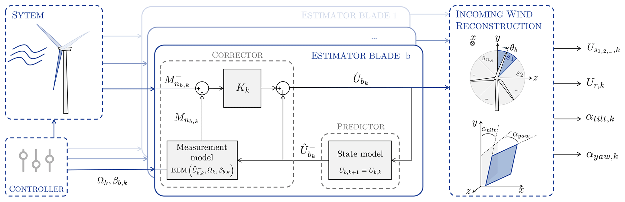
Figure 1 Block diagram of the blade-load-based estimator relying on the BEM as an internal model and on an extended Kalman filter as an estimator; each blade has its own estimator. The blade-effective wind speeds are mapped to the fixed frame in the wind reconstruction block.

2.1.2 Estimation of blade-effective wind speeds

We apply the EKF theory to the estimation of blade-effective wind speeds, considering blades to be rotating sensors whose bending moments are measured. One estimation is performed for each blade b, as shown in the block diagram of Fig. 1.

Control input. The control input vector u consists of the rotation speed of the turbine and the blade pitch angle,

$$\begin{array}{}\text{(11)}& {\mathit{u}}_k=[{\mathrm{\Omega }}_k,{\mathit{\beta }}_{\mathrm{b},k}].\end{array}$$

State. The variable to be estimated is the blade-effective wind speed, U_b, which is an input to the wind turbine blade system. To match the EKF formalism, we model this input as a state and do not explicitly model the internal states of the system. The one-dimensional state vector is therefore

$$\begin{array}{}\text{(12)}& x_k=U_{\mathrm{b},k}.\end{array}$$

State function. The state evolution is modeled as a random walk with process noise w:

$$\begin{array}{}\text{(13)}& U_{\mathrm{b},k}=f\left(U_{\mathrm{b},k-\mathrm{1}}\right)+w_{k-\mathrm{1}}=U_{\mathrm{b},k-\mathrm{1}}+w_{k-\mathrm{1}}.\end{array}$$

Considering a random walk is equivalent to assuming that the estimated state is a bias because the expected value is a constant. Using a random walk to model the evolution of the state is thus a simplification in this case, as the blade-effective wind speed is expected to be periodic with a 1P component. A model representation accounting for the 1P periodicity of the blade-effective wind speed as the one proposed in van Vondelen et al. (2023a) would better represent the system dynamics. Yet, the random walk was successfully used in the context of blade-effective wind speed estimation in Bottasso et al. (2018) and Brandetti et al. (2023) because the 1P variations are slow compared to the estimation time step and can thus be captured.

Measurement function. The state is estimated based on the measurements of the blade out-of-plane bending moments, $M_{n_{\mathrm{b}}}$. We model the system using the BEM theory, and hence the nonlinear output equation is

$$\begin{array}{}\text{(14)}& {\displaystyle }{M}_{n_{\mathrm{b},k}}=h\left(U_{\mathrm{b},k},[{\mathrm{\Omega }}_k,{\mathit{\beta }}_{\mathrm{b},k}]\right)+v_k,\text{(15)}& {\displaystyle }=\mathrm{BEM}\left(U_{\mathrm{b},k},[{\mathrm{\Omega }}_k,{\mathit{\beta }}_{\mathrm{b},k}]\right)+v_k.\end{array}$$

Note that the original version of the BEM theory is based on the conservation of momentum in a stream tube flowing through the rotor (Hansen, 2015). Therefore, it runs under the assumption of rotor-effective quantities. Appendix A shows how the BEM is used to return individual blade loads from blade-effective velocities. Another key assumption of the classical BEM theory, which we further refer to as static BEM, is that the wake is fully developed and that the induction of the rotor is then (quasi-)steady (Hansen, 2015). In Sect. 4.3.2, we will show how this BEM model can be modified to account for the induction changes generated by the pitch control strategies considered in this paper.

Noise covariance matrices. Several combinations of process noise covariance and measurement noise covariance are tested to determine the best configuration. The values leading to the smallest estimation errors and avoiding excessive filtering are $Q^{*}=Q/(U^{*}{)}^{\mathrm{2}}=\mathrm{0.1}$ and $R^{*}=R/(M_n^{*}{)}^{\mathrm{2}}=\mathrm{0.0001}$, where U^* and $M_n^{*}$ represent the order of magnitude of the incoming wind speed and bending moments, respectively.

Jacobian matrices. The expression of the Jacobian matrix for the state function is trivial: F_k=1.

As the BEM is an iterative method (see Appendix A), an analytical expression of the Jacobian matrix for the measurement function cannot be provided. We therefore numerically compute it using central finite differences, with ΔU a constant value tuned manually, following

$$\begin{array}{}\text{(16)}& H_k={\displaystyle \frac{h({\widehat{U}}_{\mathrm{b},k}^{+}+\mathrm{\Delta }U,[{\mathrm{\Omega }}_k,{\mathit{\beta }}_{\mathrm{b},k}\left]\right)-h({\widehat{U}}_{\mathrm{b},k}^{+}-\mathrm{\Delta }U,[{\mathrm{\Omega }}_k,{\mathit{\beta }}_{\mathrm{b},k}\left]\right)}{\mathrm{2}\mathrm{\Delta }U}}.\end{array}$$

Note that this procedure requires two more BEM evaluations. Opting for forward finite differences, for example, could save one evaluation if computational time was to become an issue.

2.1.3 Reconstruction of the incoming wind

The procedure described above considers the estimation of the blade-effective wind speeds that are naturally expressed in the blade rotating frame. They are further manipulated to provide information about the incoming flow in the fixed frame. We also want the information to be provided at a local scale in order to capture turbulent and shear patterns in the wind. The rotor is then divided into a chosen number of sectors, n_S, and we map the blade-effective wind speeds to the sector-effective wind speeds (see Fig. 1). A sector-effective wind speed U_s is the mean blade-effective wind speed seen by the blade as it travels across a sector s. A sector-effective wind speed is updated every time a blade leaves that sector, i.e., at a 3P frequency. The update procedure is formally given in Appendix B. At every instant, the rotor-effective wind speed is computed as the average velocity of the n_S sectors.

The wind field can also be synthesized as a sheared plane (see Fig. 1). This provides a representation of the shear present in the atmospheric boundary layer through a tilting shear coefficient α_tilt, but also gust- or wake-generated shear in the yaw direction α_yaw. The least-square approximation is used to find the expression of the plane best fitting the sector-effective wind speeds. Following derivations in Bottasso et al. (2018), sector-effective wind speeds are assumed to account for the wind speed at $r=\mathrm{2}R/\mathrm{3}$. The target expression for the velocity field is

$$\begin{array}{}\text{(17)}& U(y,z)=U_r+{\mathit{\alpha }}_{\mathrm{tilt}}y+{\mathit{\alpha }}_{\mathrm{yaw}}z,\end{array}$$

with y the vertical direction and z the transverse one.

2.2 Simulation environment

The estimator is verified numerically. Simulations are performed with an in-house LES environment (Chatelain et al., 2017; Balty et al., 2020; Coquelet et al., 2022). The Navier–Stokes equations are solved by a vortex particle mesh (VPM) method (Chatelain et al., 2013) and wind turbine blades are modeled by immersed lifting lines (Caprace et al., 2019). The code is coupled to the multi-body-system solver ROBOTRAN that handles the dynamics of the rigid rotor (Docquier et al., 2013). Turbulence is injected at the inflow using Mann boxes (Mann, 1998). Wind shear can be modeled at the inflow through the following power law:

$$\begin{array}{}\text{(18)}& {\displaystyle \frac{U\left(y\right)}{U_{\mathrm{hub}}}}={\left({\displaystyle \frac{y}{H_{\mathrm{hub}}}}\right)}^{\mathit{\alpha }},\end{array}$$

where y is the vertical elevation from the ground, H_hub and U_hub are the hub height and velocity, respectively, and α is the shear coefficient.

3 Validation of the estimator for a single turbine in turbulent flows with no shear

In this section, the estimator is validated for an isolated turbine operating in turbulent wind. The numerical setup is first presented, and the results are then discussed.

3.1 Numerical setup

The estimator is validated using the NREL 5 MW (Jonkman et al., 2009) wind turbine, characterized by a rotor diameter D=126 m, a rated wind speed of 11.4 m s⁻¹, and a rated rotor speed of 12.1 rpm. For this validation study, we consider three mean infinite upstream wind speeds U_ref: 5, 9, and 14 m s⁻¹. For each wind speed, we consider three turbulence intensity (TI) levels: 6 %, 10 %, and 15 %. Shear is not present in these simulations and no controller is active: the turbine operates at a prescribed rotation speed and collective pitch angle following Jonkman et al. (2009).

The boundary conditions are inflow–outflow in the streamwise direction, x, and unbounded in the vertical, y, and transverse, z, directions. The extent of the computational domain is $\mathrm{8}D\times \mathrm{4}D\times \mathrm{4}D$ with a $D/\mathrm{64}$ spatial resolution. The LES time step is adaptive and the operating parameters of the turbine are sampled at a 10 Hz frequency to feed the EKF.

An adjunct LES in which no turbine is present is also performed for each wind case. The quantities estimated by the EKF can then be assessed by comparing them to the “ground truth”, as the additional simulations provide an unambiguous definition of the freestream quantities. The rotor-effective wind speeds are computed as the average, over a disk located at the position of the rotor in the original simulation, of the streamwise velocity extracted from the adjunct LES. This is formally computed as

$$\begin{array}{}\text{(19)}& U_{r,k}^{\mathrm{LES}}={\displaystyle \frac{\mathrm{1}}{\mathit{\pi }{R}^{\mathrm{2}}}}\underset{\mathrm{disk}}{\iint }{u}_{x,k}(x=x_{\mathrm{WT}},y,z)\mathrm{d}S,\end{array}$$

where u_x,k is the streamwise velocity field at time k, x_WT is the location of the wind turbine in the original simulation, and the spatial integral is performed over the disk area swept by the rotor blades. The formulation for the sector-effective wind speeds is similar, except for the fact that the spatial integral is performed over each sector area such that

$$\begin{array}{}\text{(20)}& U_{\mathrm{s},k}^{\mathrm{LES}}={\displaystyle \frac{n_S}{\mathit{\pi }{R}^{\mathrm{2}}}}\underset{\mathrm{sector}}{\iint }{u}_{x,k}(x=x_{\mathrm{WT}},y,z)\mathrm{d}S.\end{array}$$

The tilt and yaw shear coefficients, ${\mathit{\alpha }}_{\mathrm{tilt},k}^{\mathrm{LES}}$ and ${\mathit{\alpha }}_{\mathrm{yaw},k}^{\mathrm{LES}}$, are retrieved from the sector-effective wind speeds using the least-square fit approach as described in Eq. (17).

3.2 Results

The rotor is discretized into eight sectors, providing an intermediate spatial resolution in the wind speed estimates. Figure 2 shows the estimation of the sector-effective wind speed (only one sector is shown for the sake of conciseness), the rotor-effective wind speed, and the tilt and yaw shear coefficients.

The temporal evolution of the sector-effective and rotor-effective wind speeds appears to be well captured across all simulations. The same remark holds for the shear coefficients. As expected, the estimated signals present steps, as a sector velocity is only updated when a blade leaves a sector, i.e., at a 3P frequency (see Appendix B). This update procedure is also partly responsible for the delay between the estimated velocities and the reference velocities. One can also notice that the estimates tend to deteriorate as the mean upstream wind speed decreases, and this is discussed hereunder.

The estimator performances are quantified using the following indicators, with N_k the number of time steps:

$$\begin{array}{}\text{(21)}& {\displaystyle }{\mathit{ϵ}}_{U_r}^{\mathrm{abs}}\left[\mathit{\%}\right]={\displaystyle \frac{\mathrm{1}}{N_k}}\sum _k{\displaystyle \frac{\mathrm{|}{U}_{r,k}-U_{r,k}^{\mathrm{LES}}\mathrm{|}}{U_{\mathrm{ref}}}},\text{(22)}& {\displaystyle }{\mathit{ϵ}}_{U_{\mathrm{s}}}^{\mathrm{abs}}\left[\mathit{\%}\right]={\displaystyle \frac{\mathrm{1}}{n_S{N}_k}}\sum _{s,k}{\displaystyle \frac{\mathrm{|}{U}_{\mathrm{s},k}-U_{s,k}^{\mathrm{LES}}\mathrm{|}}{U_{\mathrm{ref}}}},\text{(23)}& {\displaystyle }{\mathit{ϵ}}_{U_{\mathrm{s}}}\left[\mathit{\%}\right]={\displaystyle \frac{\mathrm{1}}{n_S{N}_k}}\sum _{s,k}{\displaystyle \frac{U_{\mathrm{s},k}-U_{s,k}^{\mathrm{LES}}}{U_{\mathrm{ref}}}},\text{(24)}& {\displaystyle }{\mathit{ϵ}}_{{\mathit{\alpha }}_{\mathrm{yaw}}}\left[\mathit{\%}\right]={\displaystyle \frac{\mathrm{1}}{N_k}}\sum _k{\displaystyle \frac{\mathrm{|}{\mathit{\alpha }}_{\mathrm{yaw},k}-{\mathit{\alpha }}_{\mathrm{yaw},k}^{\mathrm{LES}}\mathrm{|}}{\frac{\mathrm{1}}{\mathrm{2}}\left({max}_k{\mathit{\alpha }}_{\mathrm{yaw},k}^{\mathrm{LES}}-{min}_k{\mathit{\alpha }}_{\mathrm{yaw},k}^{\mathrm{LES}}\right)}},\text{(25)}& {\displaystyle }{\mathit{ϵ}}_{{\mathit{\alpha }}_{\mathrm{tilt}}}\left[\mathit{\%}\right]={\displaystyle \frac{\mathrm{1}}{N_k}}\sum _k{\displaystyle \frac{\mathrm{|}{\mathit{\alpha }}_{\mathrm{tilt},k}-{\mathit{\alpha }}_{\mathrm{tilt},k}^{\mathrm{LES}}\mathrm{|}}{\frac{\mathrm{1}}{\mathrm{2}}\left({max}_k{\mathit{\alpha }}_{\mathrm{tilt},k}^{\mathrm{LES}}-{min}_k{\mathit{\alpha }}_{\mathrm{tilt},k}^{\mathrm{LES}}\right)}}.\end{array}$$

Regarding the estimation of the rotor-effective velocity, the relative absolute errors reported in Table 1 remain under 4 %, while for the sector-effective velocities, they remain under 5 %. This is similar to the errors in Bottasso et al. (2018).

Table 1 Relative errors for the estimation of the rotor-effective wind speed, the sector-effective wind speed, and the shear coefficients for the nine validation cases.

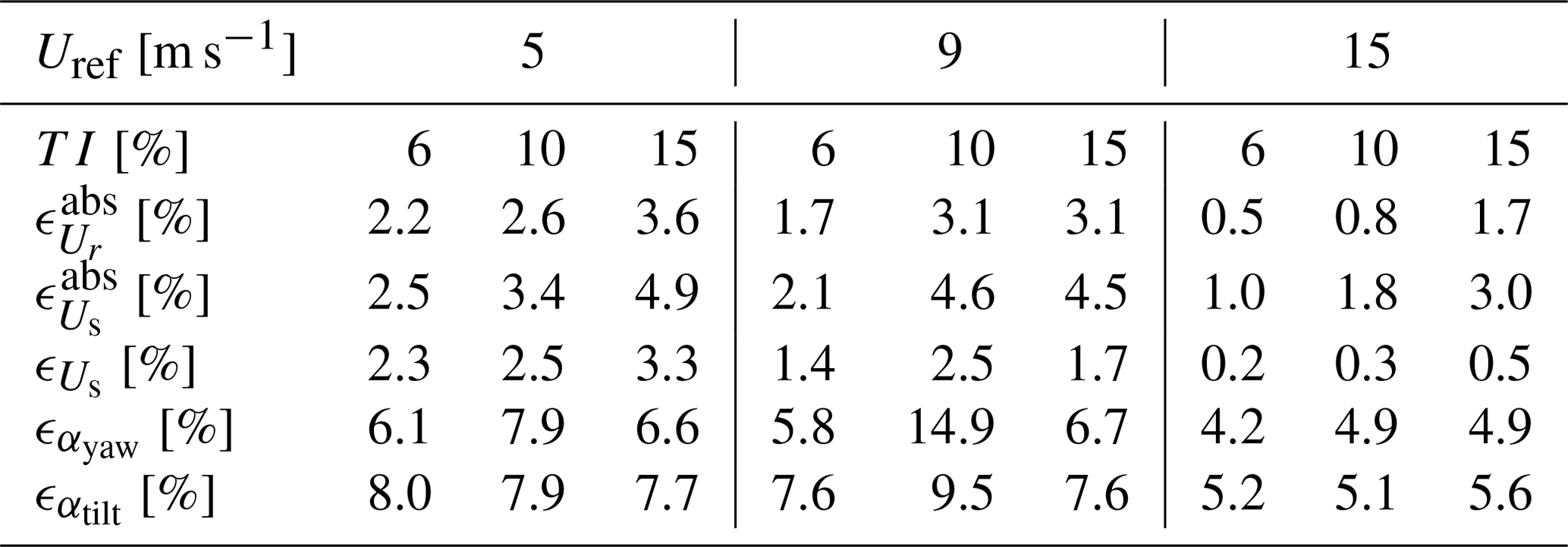
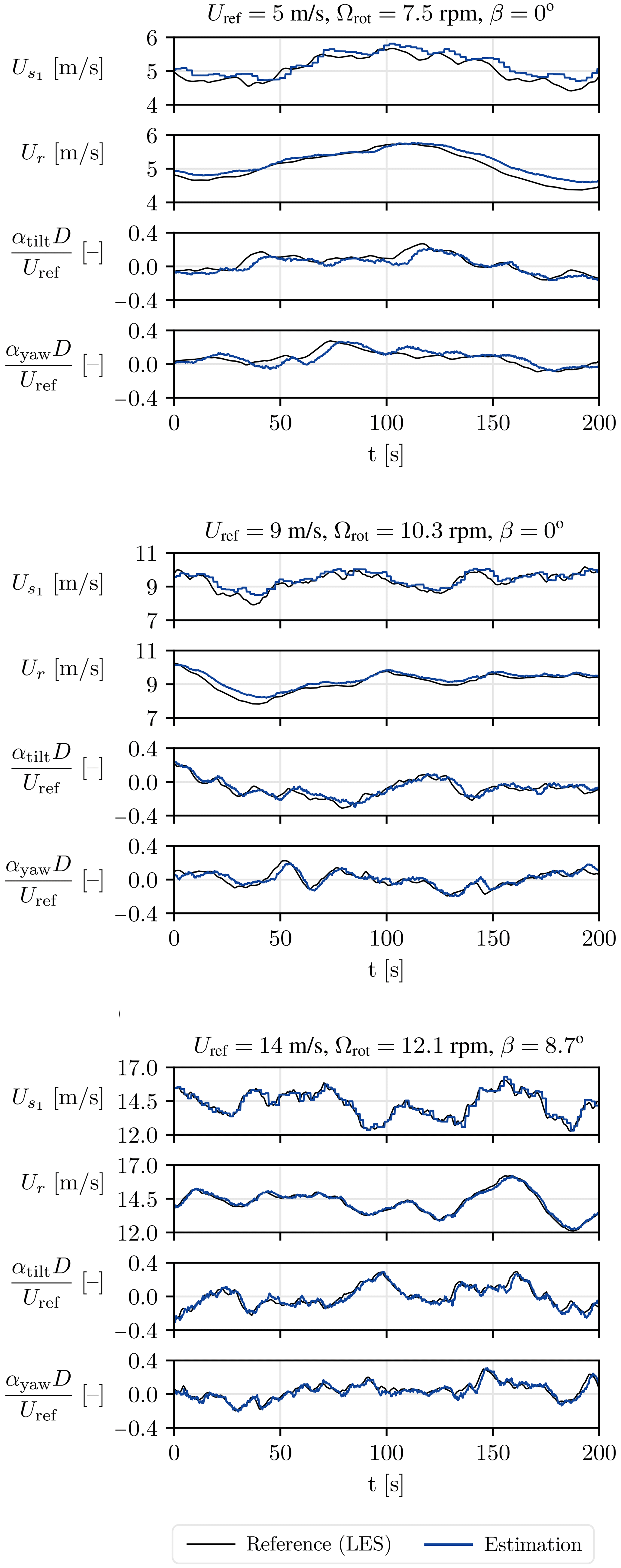
Figure 2 Estimated wind characteristics (sector-effective wind speed, rotor-effective wind speed, shear coefficients) at three wind speeds with TI=10 %: LES-recovered references (black) and estimated values (blue).

We also verify whether a bias is present in the estimation by computing ${\mathit{ϵ}}_{U_{\mathrm{s}}}$. Table 1 shows that a bias around 0.3% is present for U_ref=15 m s⁻¹ and it increases to become of the order of 2 %–2.5 % for U_ref=5 m s⁻¹. This reveals that a mismatch appears between the internal model of the estimator (the BEM) and the actual system (the LES) as the wind speed decreases. It is known from the literature that the 1D momentum theory from which the BEM is derived breaks down at low wind speeds as the rotor is heavily loaded (Hansen, 2015). As the EKF procedure consists of comparing the real output of the system to the expected output computed by the model, a bias in the model leads to a bias in the estimation.

While the absolute level of the forces is higher in the LES than in the BEM, hence the positive bias in the estimation, the dynamic changes of the system state are well captured (see Fig. 2). The estimator thus entails a great perception of the temporal and local changes in wind speed, which is what is of most interest for the control purposes targeted in this paper. If the bias was still an issue, a bias-aware EKF could be used, as suggested by Drécourt et al. (2006). A common practice is to augment the state vector of the original problem with the bias (Friedland, 1969). The EKF therefore estimates both the state and the bias, as done in the work of Pamososuryo et al. (2023) in the context of wind turbine control.

Table 1 also reveals a degradation of the error metrics as TI increases. We relate this to the spatiotemporal averaging underlying the estimation process. The reference sector-effective wind speed is the unweighted average of the flow field in the radial and azimuthal directions. The sector-effective wind speed estimated by the EKF is also the result of an averaging, but performed differently. First, the radial averaging is materialized by the blade-effective wind speed. The latter is computed by the EKF to minimize the difference between the measured bending moment (here extracted from LES) and the modeled bending moment (here obtained from the BEM). So the EKF uses the BEM to synthesize a turbulent wind speed distribution into a single blade-effective wind speed. Yet a wind turbine blade, and as a consequence the BEM, is nonlinear. Therefore the radial averaging is not simply an unweighted average. Second, the azimuthal averaging is performed by the transformation from blade-effective wind speed to sector-effective wind speed. All azimuthal information considered to get the sector average corresponds to a different instant and the estimated sector-effective wind speed is only updated at a 3P frequency. This is the limitation of using discrete blades as sensors. To summarize, the reference sector-effective wind speed at time t is a linear combination of local wind speeds at time t, while the estimated sector-effective wind speed at time t is a nonlinear combination of local wind speeds from time $t-T_{\mathrm{rot}}/\mathrm{3}$ to t. If the flow field was uniform, the averaging performed by the estimator would be equivalent to the reference averaging. But as turbulence increases, the output of the spatiotemporal averaging associated with the estimator diverges from the reference one.

4 Robustness of the estimator to active pitch control strategies

While the previous section has focused on validating the estimator, this section aims to test it in more realistic wind conditions and when controllers are active on the turbine. The choice of the study cases is motivated as described hereunder.

4.1 Controllers

The estimator presented here relies on blade loads and operating parameters. Both are influenced by the controller that is active on the wind turbine. In this section, we verify that the estimator is robust to the chosen control strategy. To do so, we propose simulations in which the three following pitch control strategies are considered: individual pitch control for load alleviation, individual pitch control for wake mixing, and collective pitch control for wake mixing. The implementation of these controllers is presented hereafter.

A baseline controller is active in all cases and serves as a comparison for the other cases. It is a classical implementation of a variable-speed, variable-pitch controller (Jonkman et al., 2009). It relies on generator torque control, maximizing the power captured below the rated wind speed, and CPC, regulating the collective pitch angle β_coll to maintain nominal power production above the rated wind speed.

For the controllers relying on individual pitch actions, the Coleman transform is used to map fixed-frame pitch commands to rotating-frame ones (Bossanyi, 2003). The individual blade pitch angles ${\mathit{\beta }}_{\mathrm{1},\mathrm{2},\mathrm{3}}$ are retrieved from the fixed-frame pitch angles, β_tilt and β_yaw, and the collective pitch angle β_coll based on the inverse Coleman transform:

$$\left[\begin{array}{c}{\mathit{\beta }}_{\mathrm{1}}\\ {\mathit{\beta }}_{\mathrm{2}}\\ {\mathit{\beta }}_{\mathrm{3}}\end{array}\right]=\left[\begin{array}{ccc}\mathrm{1}& \cos \mathit{\theta }& \sin \mathit{\theta }\\ \mathrm{1}& \cos \left(\mathit{\theta }-\frac{\mathrm{2}\mathit{\pi }}{\mathrm{3}}\right)& \sin \left(\mathit{\theta }-\frac{\mathrm{2}\mathit{\pi }}{\mathrm{3}}\right)\\ \mathrm{1}& \cos \left(\mathit{\theta }+\frac{\mathrm{2}\mathit{\pi }}{\mathrm{3}}\right)& \sin \left(\mathit{\theta }+\frac{\mathrm{2}\mathit{\pi }}{\mathrm{3}}\right)\end{array}\right]\left[\begin{array}{c}{\mathit{\beta }}_{\mathrm{coll}}\\ {\mathit{\beta }}_{\mathrm{tilt}}\\ {\mathit{\beta }}_{\mathrm{yaw}}\end{array}\right],$$

where θ is the azimuthal position of the first blade (θ=0 when the blade is pointing upward).

The IPC-based load alleviation controller, further referred to as IPC, consists of two PI controllers, one for the yaw axis and one for the tilt axis. They compute the fixed-frame pitch commands β_tilt,yaw, bringing the fixed-frame loads M_tilt,yaw to zero, in the fashion of Bossanyi (2003). More details on this specific implementation can be found in Coquelet et al. (2022).

The IPC-based wake mixing controller, further referred to as Helix, is implemented as an open-loop control strategy (Frederik et al., 2020). It imposes sinusoidal variations of the fixed-frame pitch angles, namely β_tilt=Asin (2πf_p t) and β_yaw=Acos (2πf_p t). The frequency f_p is defined by the Strouhal number $St=f_{\mathrm{p}}D/U_{\mathrm{ref}}$ based on the rotor diameter D and the wind speed U_ref. The pitch actuation generates variations of the tilt and yaw moments, eventually forcing the wake to displace laterally and vertically (see Fig. 3) and to propagate downstream as a helix, hence the name.

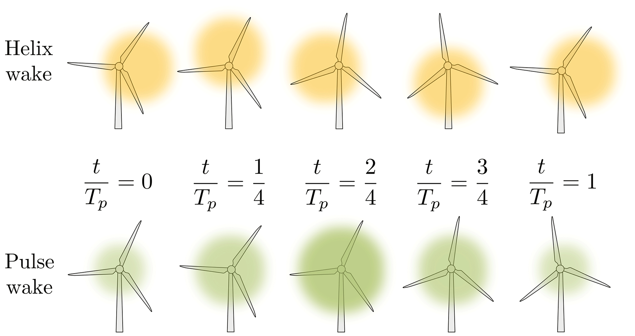
Figure 3 Simplified representation and description, over a period T_p, of the helix (yellow) and pulse (green) wakes impinging on a downstream wind turbine. The colored zone schematically represents the wake deficit and the opacity reflects its intensity, while the radius reflects its expansion.

The CPC-based wake mixing controller generates a pulsing pattern in the wake (see Fig. 3) by periodically changing the thrust force of the rotor. The position of the wake is not impacted, but its intensity and expansion change over time as a result of the changes in induction. We further refer to this strategy as the Pulse. It is implemented as a superimposition of low-frequency harmonic oscillations onto the collective pitch angle β_coll computed by the baseline controller. The pitch angle evolution is thus dictated by

$$\begin{array}{}\text{(26)}& {\mathit{\beta }}_{\mathrm{1}}={\mathit{\beta }}_{\mathrm{2}}={\mathit{\beta }}_{\mathrm{3}}={\mathit{\beta }}_{\mathrm{coll}}+A\sin \left(\mathrm{2}\mathit{\pi }St{\displaystyle \frac{U_{\mathrm{ref}}t}{D}}\right).\end{array}$$

4.2 Numerical setups

We perform the LES of a pair of in-line NREL 5 MW turbines with a 5 D spacing (Fig. 4a) such that the estimator can be tested on a freestream turbine but also on a waked turbine. The boundary conditions are inflow–outflow in the streamwise direction x, slip wall in the vertical direction y, and periodic in the transverse direction z. The numerical domain extent is $\mathrm{12}D\times \mathrm{3}D\times \mathrm{8}D$, and the spatial resolution is $D/\mathrm{32}$.

Figure 4 Horizontal and vertical slices of the instantaneous streamwise velocity field used to retrieve bending moments to feed the estimator (a) and simulations used as a reference to verify the wind speed estimates for the first (b) and second (c) turbines. Only the 9 m s⁻¹ baseline control case is shown.

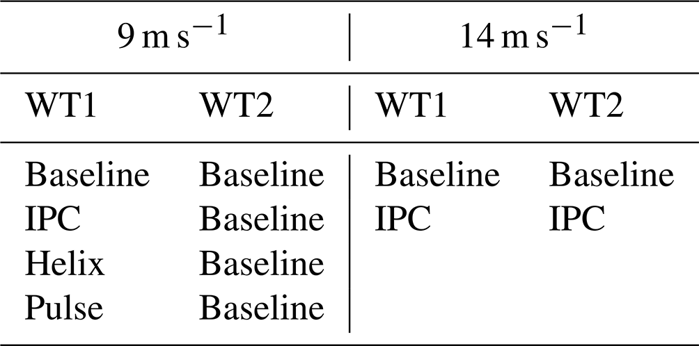
The inflow wind is sheared (α=0.2) and turbulent (TI =6 %) in order to represent atmospheric boundary layer flows. Two wind speeds are considered: 9 and 14 m s⁻¹. For the 9 m s⁻¹ cases, both turbines operate in under-rated conditions: this is representative of a configuration in which wake mixing control would be applied. On the first turbine, we therefore test the baseline controller, the Pulse, the Helix, and IPC for the sake of completeness, even though it is usually not used at below-rated wind speeds. The downstream turbine is always operated using the baseline controller. We opt for commonly used parameters for both the Helix and the Pulse (Frederik et al., 2020; Munters and Meyers, 2018): St=0.25 and A=2.5°. Note that, as both turbines operate at under-rated wind speed, only the generator torque control is active for the baseline controller such that the collective pitch control is β_coll=0. For the 14 m s⁻¹ cases, both turbines operate in above-rated conditions. There would be no point in using wake mixing control in that case, and hence it is not tested. Conversely, this is a configuration in which both the upstream and downstream turbines would use load alleviation control. We therefore consider two cases: baseline controller on both turbines and IPC on both turbines. In both cases, collective pitch control is used by the baseline controller for power regulation. When load alleviation control is switched on, the individual pitch commands are added on top of the collective pitch command, following the Coleman transform. Table 2 summarizes the abovementioned cases.

Table 2 Summary of the configurations tested to investigate the robustness of blade-load-based estimator to active pitch control.

The wind speed estimation for both the upstream and the downstream turbine is performed at a 10 Hz frequency. For the upstream one, the reference velocities are defined as the velocity from a slice located at the rotor position when the rotor is not present (Fig. 4b). When it comes to the downstream turbine, the reference velocities are accordingly retrieved from simulations of each control case in which only the first turbine is present (Fig. 4c). The reference velocities are computed following Eqs. (19) and (20).

4.3 Under-rated conditions: 9 m s⁻¹

The under-rated condition cases are discussed in this section. The impact of the control strategy is first highlighted, and then an adaptation of the BEM accounting for dynamic pitch actuation is proposed. Results for the upstream and downstream turbines are presented.

4.3.1 Impact of the control strategy on operating parameters and measured loads

Figure 5 shows the impact of the controller on the operating parameters and the out-of-plane moments. The baseline case shows that, if the pitch is equal for all blades, the effect of shear and turbulence generates 1P oscillations (period T_rot) on the blade bending moments.

When IPC is used, the changes in wind speed perceived by the blade as it rotates are compensated for by the pitch actuation. These vary individually at the 1P frequency, and the amplitude of the actuation varies with time as the controller is closed-loop.

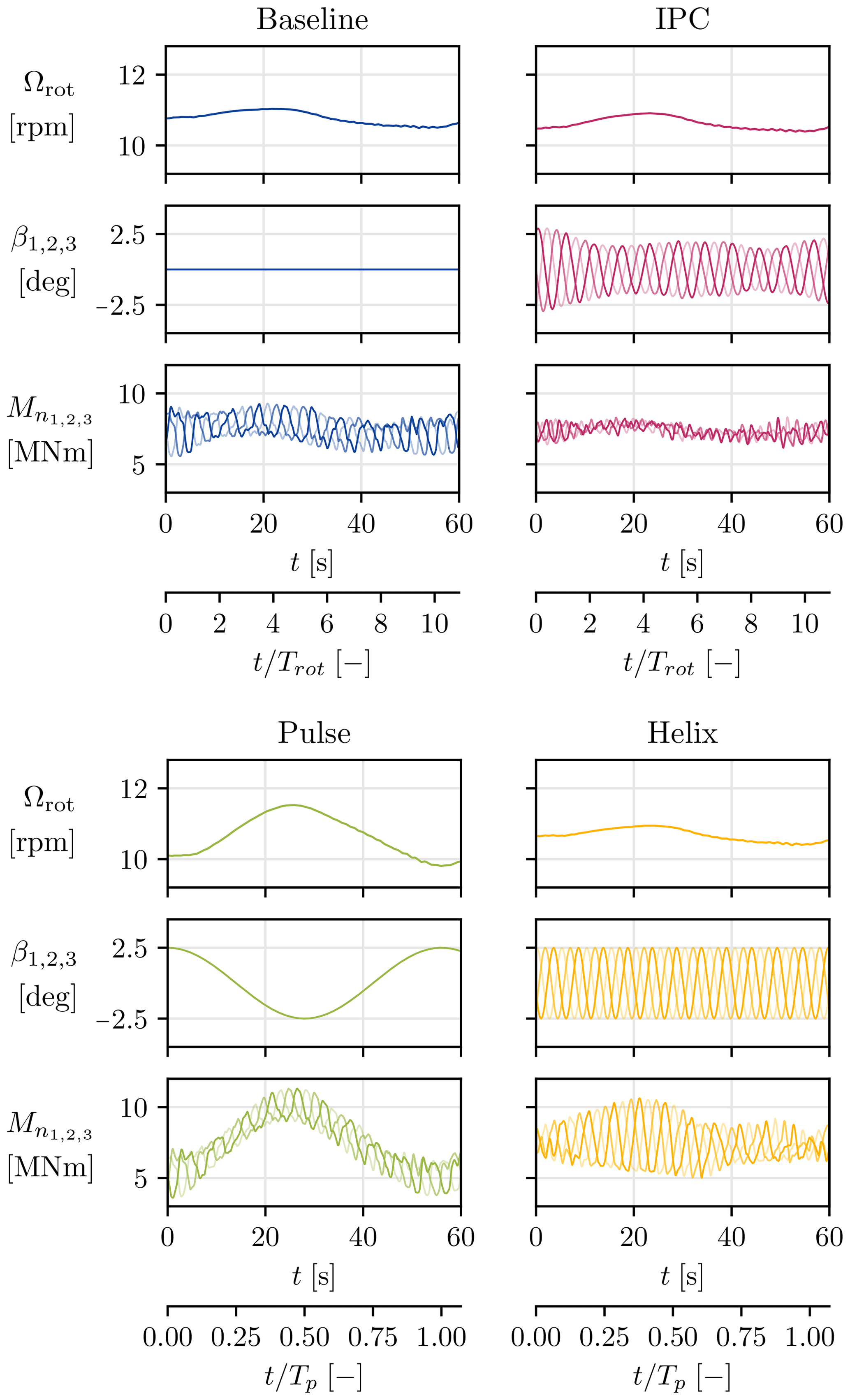
Figure 5 Effect of the control strategy on rotation speed, blade pitch angles, and out-of-plane bending moment. One color shade is used for each blade. The time axis is given in seconds and rotation periods T_rot for the baseline and IPC controllers as the dominant effects are observed at 1P in those cases. For the Pulse and Helix cases, time is made dimensionless using the actuation period T_p.

For the Pulse case, all blades are pitched at the same angle. Given the Strouhal number of 0.25, the actuation period T_p is about 10 times the rotation period. The amplitude of the pitch oscillations is constant as the strategy is open-loop. The mean value of the out-of-plane moments is marked by this periodicity and displays the changes in rotor induction.

For the Helix case, it comes from the Coleman transform that the pitching frequency is $\mathrm{1}/T_{\mathrm{rot}}+\mathrm{1}/T_{\mathrm{p}}$ (see Frederik et al., 2020, for derivation), while the pitching amplitude is constant. This does not impact the mean value of the bending moments, as the individual pitch action is performed in a three-phase manner, with a 120° offset between each blade. Rather, the effect is also visible in the amplitude of the bending moments, which is sometimes increased (around t=20 s in Fig. 5) and sometimes decreased (around t=50 s in Fig. 5). The effect is better understood looking at tilt and yaw moments, as those become quadrature-phase sinusoidal signals with a $\mathrm{1}/T_{\mathrm{p}}$ frequency.

This section has highlighted how the control strategies considered in this work impact the state of the turbine, i.e., its operating parameters and the loads it experiences. This further motivates the need to verify the robustness of the blade-load-based estimator to the pitch control strategy active on the turbine. It also points at verifying the accuracy of the BEM in scenarios that involve dynamic actuation.

4.3.2 Handling effects of dynamic actuation in the BEM

In the current formulation of the estimator, the internal model relies on the BEM theory. As discussed before, the standard BEM maps the operating parameters of the turbine and the wind speed to the forces exerted on the blades, and the mapping is static. This comes from the assumption of the BEM that the wake is fully developed, which underlies that the induction of the blades and thus the induced velocities around them are (quasi-)steady. Yet the Pulse and the Helix inherently generate periodic variations of the induction, and hence the wake is never fully developed. Through the collective pitch actuation, the Pulse changes the induction of the entire rotor. When it comes to the Helix, the individual pitch actuation changes the local induction of each blade. A time delay therefore exists before equilibrium is reached between the induction factors and the aerodynamic loads. In order to account for it, we propose making use of a dynamic formulation for the BEM based on the work of Snel and Schepers (1995). Appendix A presents how the quasi-steady normal, a, and tangential, a^′, induction factors are computed. From these induction factors, the quasi-steady induced velocities, normal w_n and tangential w_t, are recovered as ${\mathit{w}}_{\mathrm{qs}}=[w_{\mathrm{n}},w_{\mathrm{t}}]=[a{U}_{\mathrm{0}},a^{\prime }{\mathrm{\Omega }}_{\mathrm{rot}}r]$, where U₀ is the infinite upstream velocity and r is the local radius of the considered blade section (see Fig. A1).

Following Snel and Schepers (1995), the induced velocities are filtered with the following first-order differential equations:

$$\begin{array}{}\text{(27)}& {\displaystyle }{\mathit{w}}_{\mathrm{int}}+{\mathit{\tau }}_{\mathrm{1}}{\displaystyle \frac{\mathrm{d}{\mathit{w}}_{\mathrm{int}}}{\mathrm{d}t}}={\mathit{w}}_{\mathrm{qs}}+k_{\mathrm{1}}{\mathit{\tau }}_{\mathrm{1}}{\displaystyle \frac{\mathrm{d}{\mathit{w}}_{\mathrm{qs}}}{\mathrm{d}t}},\text{(28)}& {\displaystyle }\mathit{w}+{\mathit{\tau }}_{\mathrm{2}}{\displaystyle \frac{\mathrm{d}\mathit{w}}{\mathrm{d}t}}={\mathit{w}}_{\mathrm{int}},\end{array}$$

where w_int is a working variable, k₁=0.6 is a constant, and τ₁ and τ₂ are time constants.

The corrected induction factors are retrieved from the corrected induced velocities $\mathit{w}=[w_{\mathrm{n}},w_{\mathrm{t}}]$ following

$$\begin{array}{}\text{(29)}& [a,a^{\prime }]=[w_{\mathrm{n}}/U_{\mathrm{0}},w_{\mathrm{t}}/({\mathrm{\Omega }}_{\mathrm{rot}}r\left)\right].\end{array}$$

We further refer to the BEM without dynamic effects as the static BEM and to the one enhanced with dynamic effects as the dynamic BEM. The tunable time constants τ₁ and τ₂ for the dynamic BEM are calibrated against LES data. To do so, we perform the simulation of the NREL 5 MW in uniform inflow with no shear at U_ref=9 m s⁻¹ when the Pulse and the Helix are active. The turbine rotation speed and blade pitch angles determined by the controller in the LES framework are retrieved and fed to the static and dynamic BEM. We recall that the immersed lifting line method used to compute aerodynamic forces in the LES intrinsically accounts for dynamic effects in the induction and is thus the reference.

Figure 6 compares, over one period T_p, the BEM values with those provided by the LES for the local induction and the out-of-plane bending moment.

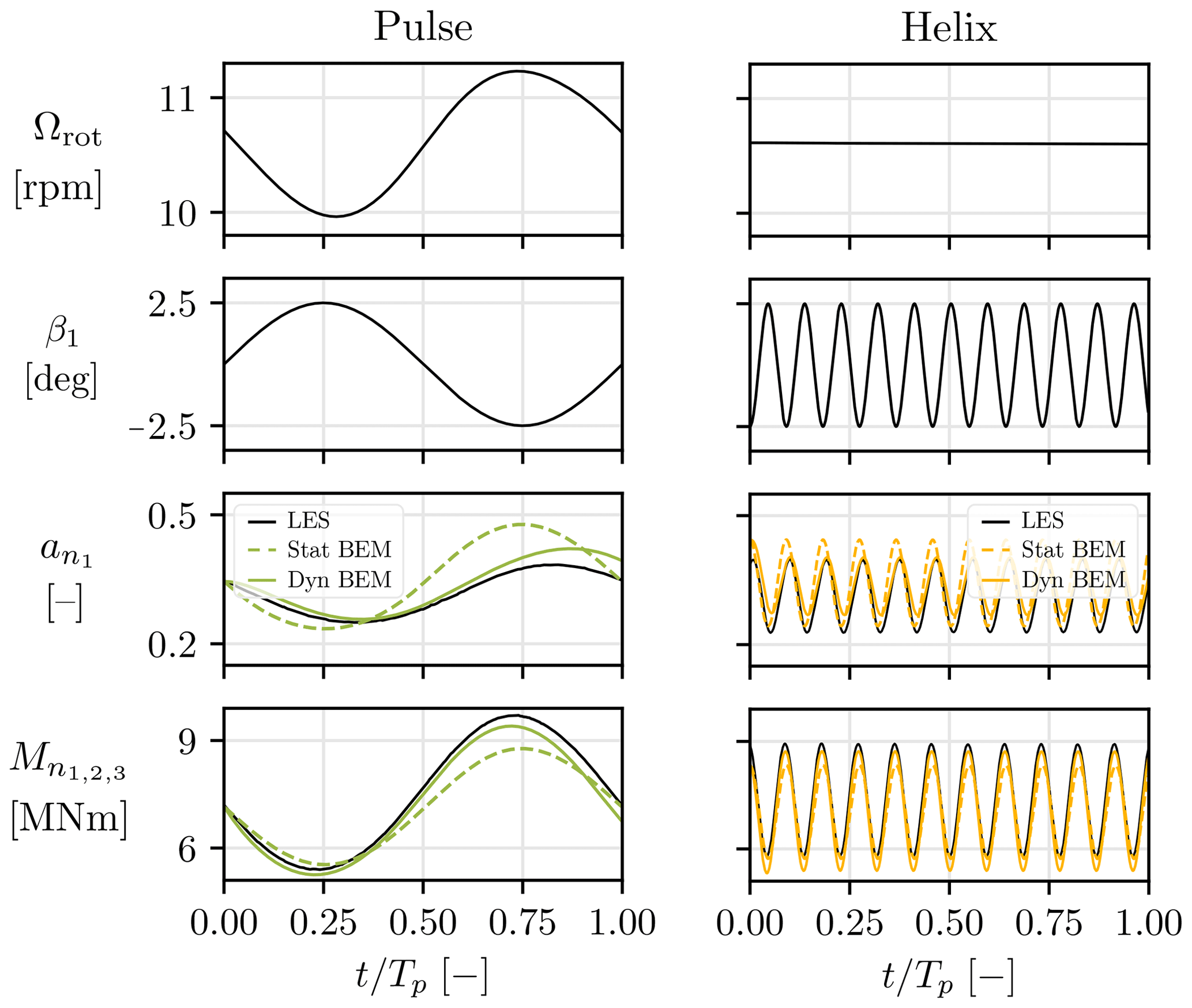
Figure 6 Comparison of LES (solid black), static BEM (dashed colored), and dynamic BEM (solid colored) in the evaluation of the local forces acting on the airfoil located at $r/R=\mathrm{3}/\mathrm{4}$ for the NREL 5 MW operated in uniform flow with U_ref=9 m s⁻¹.

It shows that, with the static BEM, the axial induction is in direct phase opposition with the pitch angle. It behaves as if, as soon as the pitch angle increases, the induced velocities are reduced. When considering the dynamic effects, a certain delay appears, which is different for the Pulse and the Helix.

Based on the analytical expression provided in Hansen (2015), we propose the following tuning of the time constants:

$$\begin{array}{}\text{(30)}& {\displaystyle }{\mathit{\tau }}_{\mathrm{1}}& {\displaystyle }={\displaystyle \frac{\mathrm{1}}{\mathrm{7}(\mathrm{1}-\mathrm{1.3}a)}}{\displaystyle \frac{\mathrm{1}}{f_{\mathrm{pitch}}}},\text{(31)}& {\displaystyle }{\mathit{\tau }}_{\mathrm{2}}& {\displaystyle }=\left(\mathrm{0.39}-\mathrm{0.26}{\left({\displaystyle \frac{r}{R}}\right)}^{\mathrm{2}}\right){\mathit{\tau }}_{\mathrm{1}},\end{array}$$

with R the rotor radius.

TSR being the tip speed ratio, we recall that the pitching frequency of the blade f_pitch is

$$\begin{array}{}\text{(32)}& {\displaystyle }{f}_{\mathrm{pitch}}^{\mathrm{Pulse}}=f_{\mathrm{p}}=St{\displaystyle \frac{U_{\mathrm{ref}}}{D}},\text{(33)}& {\displaystyle }{f}_{\mathrm{pitch}}^{\mathrm{Helix}}=f_{\mathrm{rot}}+f_{\mathrm{p}}=\left({\displaystyle \frac{\mathrm{TSR}}{\mathit{\pi }}}+St\right){\displaystyle \frac{U_{\mathrm{ref}}}{D}}.\end{array}$$

This section therefore shows that ignoring the delays leads to poor evaluation of the angle of attack, which eventually leads to inaccurate loads. Including dynamic effects in the BEM therefore increases the accuracy of the internal model of the estimator, which should improve the quality of the estimate provided by the EKF.

4.3.3 Results for the upstream turbine

We divide the rotor into four sectors (n_S=4) placed as a cross, which leads to a top, right, bottom, and left sector. This allows us to capture the effects of shear thanks to the top–bottom differences and the effects of gust or wake impingement through the left–right imbalances. We first comment on the results of the estimator in its original formulation, i.e., using the static BEM. Time series of the rotor-effective and sector-effective wind speeds are provided in Fig. 7, along with their power spectral density (PSD).

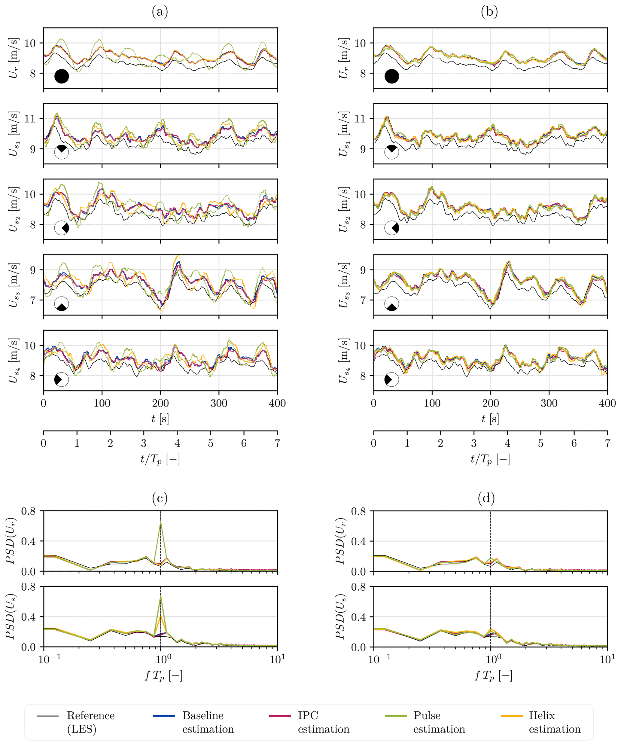
Figure 7 9 m s⁻¹ case: wind speed estimation on the upstream turbine (WT1) using a static (a, c) and dynamic (b, d) BEM as the internal model in the EKF. Time series of the estimated wind speeds (a, b) and their power spectral density (c, d) are presented. Reference velocities (black) are extracted from the LES. The wind speeds are estimated by the upstream turbine, which is operated with four different control strategies: baseline (blue), IPC (red), Pulse (green), and Helix (yellow).

When it comes to the rotor-effective wind speed, the estimations are almost identical for the baseline, IPC, and Helix cases. When the Pulse is active on the turbine, oscillations appear in the wind speed estimate at the Pulse frequency. For the sector-effective wind speed, these oscillations are present not only for Pulse but also for Helix.

This highlights that neglecting the dynamic effects in the internal model of the system, as is done with the look-up table approaches in Bottasso et al. (2018), Liu et al. (2021), and Liu et al. (2022), is inadequate for the considered application. When the static BEM is used, the expected measurement provided by the internal model in the EKF is not accurate. There is a mismatch with the actual measurement, and the wind speed estimate is wrongfully corrected in the correction step. For the Pulse, this leads to periodic oscillations of both the rotor-effective wind speed and the sector-effective wind speed at the actuation frequency $\mathrm{1}/T_{\mathrm{p}}$. With the Helix control, the changes in induction are performed individually at each blade in a three-phase manner, with a 120° offset between each blade. The inaccurate oscillations therefore appear on the blade-effective wind speeds, but they cancel out at the rotor scale.

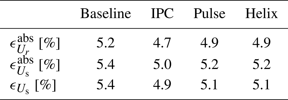
Figure 7 presents the result of the estimators once dynamics are taken into account in the internal BEM model. The estimates are now identical whatever the control strategy active on the turbine: the adapted estimator is robust to the control strategy. The capacities of the estimator described in Sect. 3 and demonstrated by several studies in the literature are then retrieved. The estimator is able to recover the higher velocities in the top sector, the intermediate ones in the left and right sectors, and the lower ones in the bottom sector. It is thus able to capture turbulence, shear, and gusts. The estimation errors are reported in Table 3 and are close to 5 %.

Figure 8 9 m s⁻¹ case: wind speed estimation on the downstream turbine (WT2), operated with baseline control, using a static BEM as an internal model in the EKF. Time series of the estimated wind speeds (a, b, c) and their power spectral density (d, e, f) are presented. Reference velocities (black) are extracted from the LES with the sole upstream turbine operated with several control strategies: baseline (blue), Pulse (green), and Helix (yellow).

Table 3 9 m s⁻¹ case: wind speed estimation errors for the upstream turbine (WT1).

The overestimation bias discussed in Sect. 3 is also observed, yet it is around 5 % here, while it was around 1.5 %–2 % in the validation case at the same 9 m s⁻¹ wind speed. We attribute this increase in bias to the setup used for the simulations. Indeed, to maintain affordable computational costs, the spatial resolution used for the LES is coarsened to $D/\mathrm{32}$, while the resolution was 2 times finer in Sect. 3. It is known that the forces computed by the LES increase when the resolution decreases due to poor capture of the tip losses (Moens et al., 2018). The mismatches between the internal model (BEM) and the actual system (LES) are higher with the simulations in this section than with those from Sect. 3. In the correction step, the EKF therefore corrects the velocity to a higher value than it should. As suggested before, this could be corrected with bias estimation (Friedland, 1969).

4.3.4 Results for the downstream turbine

The Pulse and the Helix are wake mixing control strategies, which means that their purpose is to modify the wake. Namely, the Pulse is expected to generate a pulsing sequence in the wake, with alternating zones of lower and higher velocities, while the Helix laterally and vertically displaces the wake as it propagates downstream (see Fig. 3). In this section, we want to verify the performances of the estimator in waked flows and its ability to capture the frequency content added to the wake by the Pulse and the Helix.

Figure 8a shows that the estimator performs reasonably well in waked conditions, capturing the large-scale changes in the wind. Yet, the estimation somewhat deteriorates compared to the upstream turbine case, as Table 4 reports. Two reasons can be mentioned to support the bigger discrepancies and stem from the inherent characteristics of a wind turbine wake: reduced velocity and higher turbulence. On the one hand, the flow dynamics are harder to capture due to the complexity and randomness of turbulence. On the other hand, the BEM loses accuracy at lower velocity, hence the bigger bias present in the estimation (6 % on average against the 5 % for the freestream turbine).

Table 4 9 m s⁻¹ case: wind speed estimation errors for the downstream turbine (WT2). The controller refers to the controller that is active on the upstream turbine. The downstream turbine is always operated with baseline control.

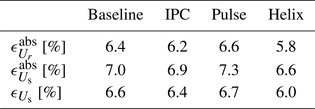
Figure 8b shows that the estimator is able to capture the frequency content added to the wake by the Pulse and the Helix control strategies. Looking back at the time series, it is also interesting to notice that the phase at which higher- and lower-velocity flow parcels are impacting a sector, or the rotor, is properly captured. This is an interesting result from the perspective of applying the Helix or the Pulse to deeper lines of turbines. The downstream turbine could therefore also be actuated with the Helix or the Pulse. To do so in an optimal way, it should synchronize its action with the periodic perturbations already present in the wake, as proposed in van Vondelen et al. (2023a) and Korb et al. (2023).

Figure 9 14 m s⁻¹ case: time series of estimated wind speeds and shear coefficients; both turbines are operated with either baseline control (blue) or IPC (red). (a) WT1 estimates for the baseline and IPC cases, (b) WT2 estimates for the baseline case, and (c) WT2 estimates for the IPC case. Reference velocities (black) are extracted from the LES.

4.4 Above-rated conditions: 14 m s⁻¹

This final section discusses the above-rated wind speed cases. The impact of using IPC on the pitch angle and blade loads is highlighted in Fig. 5 and is not shown here. Note, however, that CPC is active in these wind conditions. Figure 9 shows the time series of the wind speed estimates for the two turbines. The static BEM is used as the internal model. Separate panels are used for the downstream turbine as the wake is somewhat different depending on whether IPC is used on the upstream turbine or not (Wang et al., 2020). The reference wind speed is thus slightly different for the two cases, as can be observed when carefully looking at Fig. 9. Instead of showing all sector-effective wind speeds as in the previous sections, Fig. 9 rather presents the horizontal and vertical shear coefficient (Eq. 17), as these quantities are specifically insightful for load alleviation control using IPC.

First, results show that the static BEM is sufficient in these cases. CPC for power regulation is active in the baseline case and additional individual pitching is added on top of it in the IPC case. Still, no rapid changes in induction are associated with the two control cases; hence the static BEM is accurate in modeling the link between operating parameters, wind speed, and blade bending moments. Figure 9 also shows that the bias of the estimator is reduced for both the freestream and the waked turbine. This is quantitatively confirmed by Table 5, which shows that errors remain under 3 % for the estimated wind speeds. It is a direct consequence of the higher wind speed: the BEM is more accurate at reduced thrust coefficients and the estimation is better.

Table 5 14 m s⁻¹ case: wind speed and shear coefficient estimation errors for the two turbines (WT1 and WT2). The latter are both operated with either baseline control or IPC.

Time series also show a good capture of the shear coefficients. The vertical wind shear of the inflow is sensed (α_tilt is nonzero on average), while the horizontal shear generated by turbulent gusts is also seen (α_yaw varies around a zero mean).

5 Conclusions

This work assesses the ability of a blade-load-based wind speed estimator to accurately sense the characteristics of the incoming wind when both collective and individual pitch control is active at the turbine.

The proposed estimator relies on an extended Kalman filter, whose internal model of the system is based on the BEM theory. When power regulation CPC and load alleviation IPC are used, a state-of-the-art static BEM ensures accurate wind speed estimations by the EKF. What this paper highlights is that, when wake mixing control is used, accounting for dynamic changes in blade induction is needed. Indeed, the static BEM is not an accurate model when the Pulse or the Helix is active on the turbine, as the static BEM considers an immediate reaction of the blade loads to the pitch actuation. It ignores the unsteady effects in the wake related to the changes in induction. Including an unsteady correction in the model is the solution we propose to make the EKF robust to the controller active on the turbine. This contribution is essential if the EKF is to be used for state-feedback control, the application targeted for this tool.

Indeed, using IPC for load alleviation in complex wind conditions is still challenging and could benefit from explicit information on local wind speeds and global shear coefficients provided by the estimator. For the Pulse and the Helix controllers, sensing the incoming flow is needed for them to be used in a closed-loop manner. This would allow them to optimally phase their dynamic actuation with the dynamics of the incoming flow structures. When talking about an upstream turbine, this refers to the gusts and shear of the atmospheric boundary layer. When talking about a waked turbine, this also refers to synchronization with the added periodic content in the Helix and Pulse wakes. A direct follow-up to this work then consists of determining if the precision provided by this estimator is sufficient for these control applications, which might lead to having to deal with the bias of the estimator. This also comes along with finding a control formulation including the wind speed estimates.

Another perspective is to investigate the effects of blade flexibility on the proposed estimator. The structural dynamics of the rotor are indeed not considered in this study, as both the EKF estimator and the LESs assume a rigid rotor. Accounting for blade flexibility modifies the blade root moments in three ways: mean value, amplitude of the fluctuations, and phase of the fluctuations (Trigaux et al., 2024b). And these effects increase as the rotor diameter increases (Trigaux et al., 2024a). Further investigations are thus needed in that field, especially when the estimator is used for larger rotors.

Appendix A: Blade element momentum theory

The BEM used in this work was implemented in-house following Hansen (2015) and validated against FAST. Rotor tilt and blade cone angle are not taken into account, and the rotor is considered to be a flat disk perpendicular to the inflow. Algorithm A1 highlights the key steps of the BEM computation. The latter is performed in an iterative manner until the value of the flow angle ϕ [rad] is converged with a tolerance of $\mathrm{tol}={\mathrm{10}}^{-\mathrm{6}}$ in this case. Flow angle and other quantities of interest for the BEM are illustrated in Fig. A1. The Glauert correction is used for high induction, and, when needed, dynamic effects can be taken into account (see Sect. 4.3.2). We refer to Hansen (2015) for more details.

Algorithm A1 BEM

for Each blade section do

Radial position r, chord c

Initialize induction factors and flow angle

  a=0.5, $a^{\prime }=\mathrm{0.005}$, ${\mathit{\varphi }}_{\mathrm{new}}=\mathit{\pi }/\mathrm{2}$, ${\mathit{\varphi }}_{\mathrm{old}}=\mathit{\pi }/\mathrm{2}+\mathrm{1}$

while ${\mathit{\varphi }}_{\mathrm{new}}-{\mathit{\varphi }}_{\mathrm{old}}>\mathrm{tol}$ do

  ϕ_old=ϕ_new

Compute angle of attack and relative velocity

  $U_n=\left(\mathrm{1}-a\right)u_{\mathrm{0}}$, $U_t=\left(\mathrm{1}+a^{\prime }\right){\mathrm{\Omega }}_{\mathrm{rot}}r$

  $\mathit{\varphi }={\tan }^{-\mathrm{1}}\left(U_n/U_t\right)$

  $\mathit{\alpha }=\mathit{\varphi }-(\mathit{\beta }+\mathit{\gamma })$

  $U_{\mathrm{rel}}=\sqrt{U_n^{\mathrm{2}}+U_t^{\mathrm{2}}}$

Retrieve lift and drag coefficients from polar

  C_L=C_L(α),  C_D=C_D(α)

Compute normal and tangential force coefficients

  $C_{\mathrm{n}}=C_L\cos \mathit{\varphi }+C_{\mathrm{D}}\sin \mathit{\varphi },$ $C_{\mathrm{t}}=C_L\sin \mathit{\varphi }-C_{\mathrm{D}}\cos \mathit{\varphi }$

Compute new induction factors

  $F_{\mathrm{tip}}=\frac{\mathrm{2}}{\mathit{\pi }}\arccos \left(\exp \left(-n_B\frac{R-r}{\mathrm{2}r\sin \mathit{\varphi }}\right)\right)$

  $F_{\mathrm{hub}}=\frac{\mathrm{2}}{\mathit{\pi }}\arccos \left(\exp \left(-n_B\frac{r-R_{\mathrm{hub}}}{\mathrm{2}r\sin \mathit{\varphi }}\right)\right)$

  $\mathit{\sigma }=\frac{n_{B}c}{\mathrm{2}\mathit{\pi }r}$

  $a=\frac{\mathrm{1}}{\frac{\mathrm{4}F{\sin }^{\mathrm{2}}\mathit{\varphi }}{\mathit{\sigma }{C}_{\mathrm{n}}}+\mathrm{1}}$

  $a^{\prime }=\frac{\mathrm{1}}{\frac{\mathrm{4}F\sin \mathit{\varphi }\cos \mathit{\varphi }}{\mathit{\sigma }{C}_{\mathrm{t}}}-\mathrm{1}}$

Update flow angle

  ϕ_new=ϕ

end while

Compute local tangential and normal force

  $f_n=\frac{\mathrm{1}}{\mathrm{2}}\mathit{\rho }{U}_{\mathrm{rel}}^{\mathrm{2}}c{C}_{\mathrm{n}}$,   $f_t=\frac{\mathrm{1}}{\mathrm{2}}\mathit{\rho }{U}_{\mathrm{rel}}^{\mathrm{2}}c{C}_{\mathrm{t}}$

end for

Integrate over span to compute out-of-plane bending moment of blade b

  $M_{n,b}={\int }_{R_{\mathrm{hub}}}^{R_{\mathrm{tip}}}\left(r-R_{\mathrm{hub}}\right)f_{n,b}\mathrm{d}r$

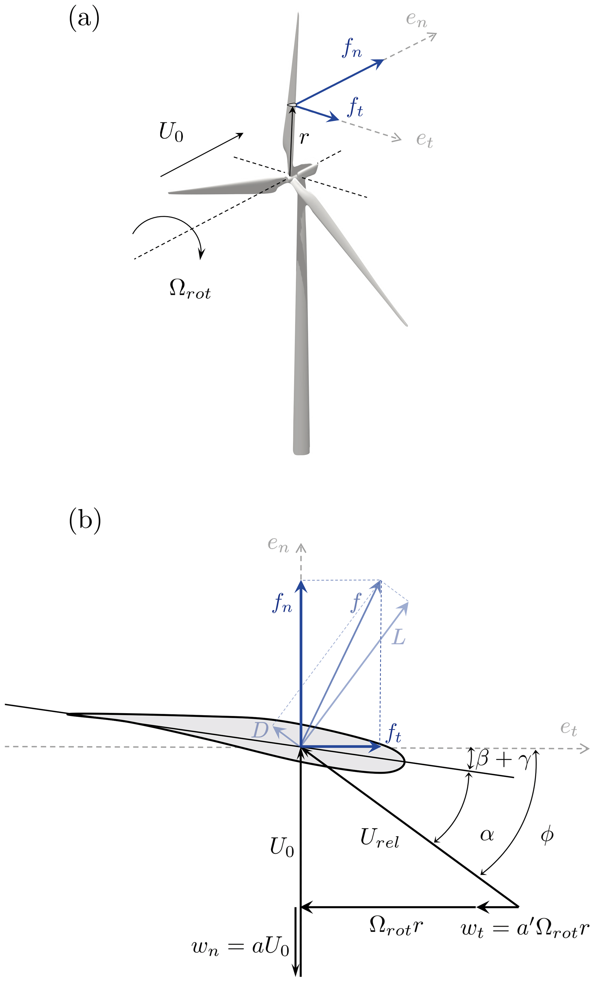
Figure A1 Reference frame for the blade forces (a) and velocity triangle at a cross-section of the blade used in the BEM (b).

Appendix B: From blade-effective wind speed to sector-effective wind speed

The rotor swept area is divided into n_S sectors of azimuthal span $\mathrm{\Delta }\mathit{\theta }=\mathrm{2}\mathit{\pi }/n_S$. Algorithm B1 formalizes the conversion from blade-effective wind speed (U_b,k) to sector-effective wind-speed (U_s,k) for a rotor with n_B blades. The second subscript stands for the time index k. The process is initiated at k=1 for each blade b by determining the sector $s_{\mathrm{b},k=\mathrm{1}}$ in which the blade is located based on its azimuthal position ${\mathit{\theta }}_{\mathrm{b},k=\mathrm{1}}$. The time history of the blade-effective wind speed is then accumulated as the blade passes through the sector using the counting variable nit_b. The wind speed of sector s is eventually updated when the blade leaves the sector s_b=s. While the blade-effective wind speeds are updated at every time index k, i.e., at the EKF estimation frequency (0.1 s in this work), the sector-effective wind speeds are only updated at a 3P frequency (around 2 s) in this context.

Algorithm B1 Transforming blade-effective wind speeds to sector-effective wind speeds.

initialization at time instant k=1

$U_{\mathrm{s},k=\mathrm{1}}=\mathrm{0}\forall s$

${\mathrm{nit}}_{\mathrm{b}}=\mathrm{1}\forall b$

$s_{\mathrm{b},k=\mathrm{1}}=\mathrm{integer}\left({\mathit{\theta }}_{\mathrm{b},k=\mathrm{1}}/\mathrm{\Delta }\mathit{\theta }\right)\forall b$

while estimation is ongoing do

$U_{\mathrm{s},k}\leftarrow U_{\mathrm{s},k-\mathrm{1}}\forall s$

for b in n_B do

$s_{\mathrm{b},k}=\mathrm{integer}\left({\mathit{\theta }}_{\mathrm{b},k}/\mathrm{\Delta }\mathit{\theta }\right)$

if $s_{\mathrm{b},k}\ne s_{\mathrm{b},k-\mathrm{1}}$ then

$s^{*}=s_{\mathrm{b},k-\mathrm{1}}$

$U_{{\mathrm{s}}^{*},k}\leftarrow \frac{\mathrm{1}}{{\mathrm{nit}}_{\mathrm{b}}}{\sum }_{\mathit{\kappa }=k-{\mathrm{nit}}_{\mathrm{b}}}^{k-\mathrm{1}}{U}_{\mathrm{b},\mathit{\kappa }}$

nit_b←1

else

${\mathrm{nit}}_{\mathrm{b}}\leftarrow {\mathrm{nit}}_{\mathrm{b}}+\mathrm{1}$

end if

end for

end while