the Creative Commons Attribution 4.0 License.
the Creative Commons Attribution 4.0 License.
 | 01 Mar 2024
Multi-objective calibration of vertical-axis wind turbine controllers: balancing aero-servo-elastic performance and noise
Sebastiaan Paul Mulders
Roberto Merino-Martinez
Simon Watson
Jan-Willem van Wingerden
Vertical-axis wind turbines (VAWTs) are considered promising solutions for urban wind energy generation due to their design, low maintenance costs, and reduced noise and visual impact compared to horizontal-axis wind turbines (HAWTs). However, deploying these turbines close to densely populated urban areas often triggers considerable local opposition to wind energy projects. Among the primary concerns raised by communities is the issue of noise emissions. Noise annoyance should be considered in the design and decision-making process to foster the social acceptance of VAWTs in urban environments. At the same time, maximising the operational efficiency of VAWTs in terms of power generation and actuation effort is equally important. This paper balances noise and aero-servo-elastic performance by formulating and solving a multi-objective optimisation problem from a controller calibration perspective. Psychoacoustic annoyance is taken as a novel indicator for the noise objective by providing a more reliable estimate of the human perception of wind turbine noise than conventional sound metrics. The computation of the psychoacoustic annoyance metric is made feasible by integrating it with an accurate and computationally efficient low-fidelity noise prediction model. For optimisation, an advanced partial-load control scheme – often used in industrial turbines – is considered, with the Kω2 controller as a baseline for comparison. Optimal solutions balancing the defined objectives are identified using a multi-criteria decision-making method (MCDM) and are subsequently assessed using a frequency-domain controller analysis framework and mid-fidelity time-domain aero-servo-elastic simulations. The MCDM results indicate the potential application of this controller in small-scale urban VAWTs to attain power gains of up to 39 % on one side and to trade off a reduction in actuation effort of up to 25 % at the cost of only a 2 % power decrease and a 6 % increase in psychoacoustic annoyance on the other side compared to the baseline. These findings confirm the flexible structure of the optimally calibrated wind speed estimator and tip-speed ratio (WSE–TSR) tracking controller, effectively balancing aero-servo-elastic performance with noise emissions and marking the first instance of integrating residential concerns into the decision-making process.
- Article
(3553 KB) - Full-text XML
- BibTeX
- EndNote


The transition from fossil fuels to sustainable energy sources is motivated by the escalating demand for energy and the imperative to curtail greenhouse gas emissions. In this context, wind energy is vital, accounting for 906 GW of global installed capacity as of 2022, with an annual growth rate of 9 % (Hutchinson and Zhao, 2023). Projections for the next 5 years anticipate 680 GW of new installed capacity with an annual growth rate of 13 %, considering both onshore and offshore locations. The offshore wind sector has garnered significant attention, primarily due to its abundant wind resources, which can be harnessed by large-scale wind turbines with an average rated output of around 8 MW connected to the grid (Ramirez, 2023). However, it is worth noting that offshore wind installation is often associated with high costs in both construction and grid connection, hindering its rapid expansion compared to onshore wind projects (Veers et al., 2019).
Onshore wind sites remain critical for the exploitation of wind energy (Watson et al., 2019). While most of this energy is generated from large-scale turbines (Veers et al., 2019), there is a growing interest in small-scale turbines due to their potential applications in urban environments (Bianchini et al., 2022). Potential integration of small rotors on tall buildings might address local renewable energy demands, complementing the push for sustainable building design (Balduzzi et al., 2012). Moreover, the importance of small-scale wind turbines extends to future distributed energy networks, especially when effectively combined with energy storage systems (Papi et al., 2021).
In this context, vertical-axis wind turbines (VAWTs) present an attractive opportunity to harness urban wind conditions, characterised by low average wind speeds and high turbulence levels, because of their ability to receive wind from any direction without requiring a yaw mechanism (Mertens et al., 2003), their simple blade design leading to cost-effective maintenance (Howell et al., 2010), and their reduced visual impact (Dayan, 2006; Khan et al., 2017) compared to the horizontal-axis wind turbines (HAWTs) dominating the urban wind energy market.
However, three main challenges remain for the urban deployment of small-scale VAWTs. The first revolves around the need to foster community engagement and social acceptance (Watson et al., 2019; Bianchini et al., 2022). Noise annoyance significantly contributes to the local opposition against urban wind energy projects (Klok et al., 2023). Measures taken to mitigate such concerns result in reduced power capture efficiency, adversely impacting revenue generation, particularly if the turbines are required to cease operation during nighttime hours (Merino-Martínez et al., 2021). To reduce the impact of such measures on the VAWT performance, an accurate prediction of the wind turbine noise impact on nearby residents is essential. This task is complex due to the influence of various factors, such as wind speed, direction, distance, and background noise (Poulsen et al., 2019). Commonly used time-averaged metrics, such as the A-weighted sound pressure level or the day–evening–night level (Lden), may not fully capture the sound properties responsible for noise annoyance (Pieren et al., 2019). Therefore, recent efforts have focused on the auralisation of environmental acoustic scenarios. Similar to its visual counterpart, this technique allows for the artificial reproduction of audible situations using numerical data (Vorländer, 2008). A notable contribution to this topic comes from the work of Merino-Martínez et al. (2021), who proposed a novel holistic approach based on synthetic sound auralisation and psychoacoustic sound quality metrics to evaluate the annoyance caused by wind turbine noise.
Turning to the second and the third challenges, optimising the controller to ensure an optimal and reliable estimation of the performance of small-scale VAWTs in turbulent and fluctuating wind conditions is paramount (Eriksson et al., 2008; Watson et al., 2019; Bianchini et al., 2022). The combined wind speed estimator and tip-speed ratio (WSE–TSR) tracking controller (Bossanyi, 2000) has been successfully applied to maximise the energy capture of VAWTs (Eriksson et al., 2013; Bonaccorso et al., 2011), demonstrating good dynamic performance in tracking the optimal operating point in turbulent wind conditions and in predicting the turbine performance. This control scheme ensures that the wind turbine operates at the maximum power coefficient associated with a particular tip-speed ratio and pitch angle (Burton et al., 2001). To track the optimal operating point and extract the maximum power, the estimated rotor-effective wind speed (REWS) (Østergaard et al., 2007; Soltani et al., 2013) is used to compute the desired rotor speed reference.
However, the optimal calibration of the WSE–TSR tracking controller is a crucial and nontrivial task due to the controller's non-linearity and high dependence on a priori model information. The first effort in providing insights into the complex dynamic of the scheme is the derivation of a linear frequency-domain framework in Brandetti et al. (2022). The work also reveals that the system is ill-conditioned, meaning that the scheme is unable to uniquely provide a wind speed estimate from the product with other internal model parameters. While the frequency-domain framework provides insights for analysing turbine controllers in terms of bandwidth, relating the linear framework to practically meaningful performance metrics (e.g. energy capture and actuation effort) remains an intricate task.
To this end, a recent study by the same authors (Brandetti et al., 2023b) focused on finding the optimal calibration of the WSE–TSR tracking controller in a multi-objective setting (Odgaard et al., 2016; Moustakis et al., 2019; Lara et al., 2023a) with power maximisation and actuation effort minimisation as conflicting objectives. The set of Pareto optimal solutions is then evaluated with a frequency-domain framework to relate performance metrics to controller insights. Results obtained using the NREL 5 MW reference HAWT (Jonkman et al., 2009) under realistic turbulent wind conditions show that when compared to the baseline Kω2 controller, an optimally calibrated WSE–TSR tracking control strategy does not enhance power capture; however, it does enable the reduction of torque actuation effort with a minor decrease in power production. This finding contradicts the expectations from the existing literature, which claimed energy capture benefits of 1 % to 3 % when applying a manually calibrated WSE–TSR tracking controller (Holley et al., 1999; Bossanyi, 2000). It should be noted that these conclusions were made more than 2 decades back and were based on the application of wind turbines that are much smaller than the NREL 5 MW turbine.
Hence, validating the above-mentioned hypothesis on a small-scale wind turbine, like an urban VAWT, holds significant interest. In the existing body of literature, numerous studies have investigated the multi-faceted aspects of small-scale turbine optimisation, particularly concerning the trade-off between minimising noise emissions and maximising power performance on HAWTs (Clifton-Smith, 2010; Sessarego and Wood, 2015; Pourrajabian et al., 2023). Despite this interest, there is a distinct lack of corresponding studies addressing these aspects in the context of VAWTs. Therefore, this paper tackles the multi-objective optimisation problem from a control perspective by balancing aero-servo-elastic turbine performance (power capture and actuation effort) with noise (psychoacoustic annoyance) for an urban VAWT. Finding a balance between these objectives will further promote the application of VAWTs in urban environments.
The 1.5 m two-bladed H-Darrieus VAWT (LeBlanc and Simão Ferreira, 2021) is chosen as a case study in the current work. The selection of this specific turbine is motivated by the availability of experimental aerodynamic data and its suitability for rooftop integration (Balduzzi et al., 2012). The psychoacoustic annoyance value needed for the optimal controller calibration is computed by coupling the perception-based approach proposed by Merino-Martínez et al. (2021) and the low-fidelity noise prediction model developed and validated against high-fidelity simulations by Brandetti et al. (2023a). As experimental acoustic VAWT data are unavailable, the aforementioned model is applied, providing the estimated noise spectra for the small-scale VAWT. These signals are subsequently auralised and assessed with psychoacoustic sound quality metrics to estimate the psychoacoustic noise annoyance.
The optimisation process explores the parameter space of the considered WSE–TSR tracking controller through a guided search procedure. Optimal solutions are identified to form the Pareto front, balancing power maximisation, actuation effort minimisation, and psychoacoustic annoyance minimisation. These optimal results are then evaluated by a linear frequency-domain system and controller analysis framework (Brandetti et al., 2023b) for comparison to the baseline Kω2 controller. Therefore, the main contributions of this paper are as follows:
-
integrating perception-based psychoacoustic sound quality metrics with a low-fidelity noise prediction model to accurately predict and characterise the acoustic emissions of a small-scale VAWT in terms of psychoacoustic annoyance
-
presenting an architecture for implementing torque control strategies in small-scale VAWTs with the mid-fidelity software QBlade (Marten, 2020) to conduct realistic aero-servo-elastic simulations of an urban VAWT
-
formulating and solving a multi-objective optimisation problem for finding the optimal calibration of the WSE–TSR tracking controller as a trade-off between acoustic and aero-servo-elastic performance for an urban VAWT and for the first time taking into account residential concerns in the decision-making process.
The paper is structured as follows: Sect. 2 derives the model for the wind turbine under study. Section 3 presents the two considered torque control strategies, namely the WSE–TSR tracking controller and the baseline Kω2 controller. Section 4 describes the combined noise prediction model and psychoacoustic annoyance model. The architecture for implementing the considered torque control strategies in QBlade and their calibration by means of multi-objective optimisation are provided in Sect. 5. The optimally calibrated WSE–TSR tracking control scheme is compared to the baseline for its performance in Sect. 6 using both the frequency-domain framework and the time-domain simulations performed with QBlade. Section 7 offers a summary of the key findings and proposes directions for future work.
This section outlines the notations used in the paper. The notations and indicate estimated quantities and time derivatives, respectively. The symbol represents values corresponding to a specific operating point but also a mean value, whereas denotes values indicating the intended optimal or reference parameters.
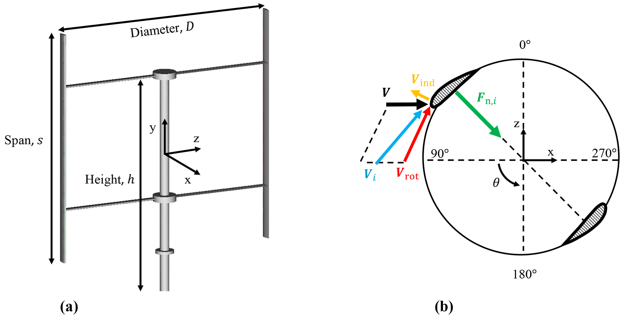
Figure 1(a) Vertical-axis wind turbine (VAWT) geometry and dimensions. The turbine is a two-bladed H-Darrieus VAWT, with diameter D, span s, and height h of dimensions equal to 1.5 m. (b) Coordinate system and definition of the rotor-effective wind speed (REWS) V, the blade-effective wind speed (BEWS) Vi, and the normal load acting on the blade per unit span Fn,i vectors adapted from De Tavernier (2021). The coordinate system is Cartesian, with the origin at the turbine centre. The blade azimuthal position θ is defined with respect to blade 1 and is considered positive in the counterclockwise direction. The vector of the BEWS Vi for the blade i results from the summation of three vector components: the REWS V, the rotational velocity Vrot of the turbine, and the induced velocity Vind. The normal force Fn,i per unit span has a positive sign when the vector points inwards.
In this section, the model for the VAWT is presented. Specifically, a two-bladed H-Darrieus turbine is considered, for which experimental aerodynamic data are available, as shown in Fig. 1a. To minimise blade deflection, two horizontal struts are used for each blade, located at approximately 25 % and 75 % of the blade length. The blades have a NACA 0021 profile with a chord length m, while the struts have a NACA 0018 profile with a chord length m. The diameter of the VAWT is D=1.5 m, with a span s and a height h, both equal to 1.5 m. These specifications are summarised in Table 1, and more detailed information about the VAWT design can be found in previous work (LeBlanc and Simão Ferreira, 2021), where the turbine was experimentally investigated.
Table 1PitchVAWT design specifications (LeBlanc and Simão Ferreira, 2021).
Figure 1b shows the turbine Cartesian coordinate system with the origin at the turbine centre. To aid in the interpretation of the results, the blade rotation is divided into two regions: the upwind region, where , and the downwind region, where . The blade azimuthal position θ is defined with respect to blade 1, and θ=90° and θ=270° represent the most upwind and downwind positions, respectively. Blade 2 lags behind blade 1 by θ=180°.
By examining the two-dimensional blade element depicted in Fig. 1b, the vector of the blade-effective wind speed (BEWS) is defined for each blade as follows:
where is the blade index for the VAWT under study; V denotes the vector for the REWS; Vrot represents the vector of the tangential velocity of the rotor, resulting from the cross-product of the vectors of the rotational speed and the radius of the turbine; and Vind is the vector of the induced velocity, caused by the force field that the turbine generates during the rotation. A detailed derivation of the BEWS can be found in De Tavernier (2021) for interested readers. In the following, the italicised notations V and Vi denote the scalar representation for the REWS and BEWS vector quantities V and Vi, respectively.
The wind turbine rotor dynamics are given by
where J is the effective low-speed shaft inertia and is derived from the relation , in which Jr and Jg are the inertia of the rotor and generator, respectively; Tg is the generator torque; and represents the gearbox ratio of the transmission, with ωg and ωr being the generator and the rotor speed, respectively. Assuming a pitch angle β constant at an angle of 0°, a value that maximises the aerodynamic efficiency for the below-rated region, the aerodynamic rotor torque can be formulated as
with ρ and Arot being the air density and the rotor area, respectively. In contrast to a HAWT, the power coefficient Cp for a VAWT is a non-linear mapping in terms of azimuth angle and tip-speed ratio,
where R represents the rotor radius. This dependency arises from the VAWT operation as the BEWS, and the angle of attack varies with the azimuth rotation angle, resulting in intrinsic three-dimensional aerodynamics (Simão Ferreira et al., 2009). These periodic and non-linear system characteristics are reflected in the dynamics of the VAWT, as illustrated in Eq. (3) and Fig. 2, where the Cp curves of the VAWT under study are plotted. The power coefficient mapping exhibits a periodicity of twice per revolution (2P) due to the turbine having two blades (Lao et al., 2022).
For a VAWT, the normal load acting on the blade per unit span, shown in Fig. 1, is defined as follows:
where Vi represents the magnitude of the BEWS for each blade. The normal load coefficient, denoted as Cn,i, is a non-linear function that depends on the tip-speed ratio and azimuthal position of blade i. It should be noted that Cn,i also varies with the blade pitch angle βi. However, βi is considered constant throughout this study, maintaining a value of 0°. Figure 3 illustrates the Cn,1 curve for the VAWT. Notably, a maximum normal load occurs at approximately θ=90°, corresponding to blade 1 being upwind. Blade 2 exhibits similar behaviour, although with a 180° shift. The variations in load dynamics throughout the rotation demonstrate the presence of a once-per-revolution periodicity (1P) in Cn,i.
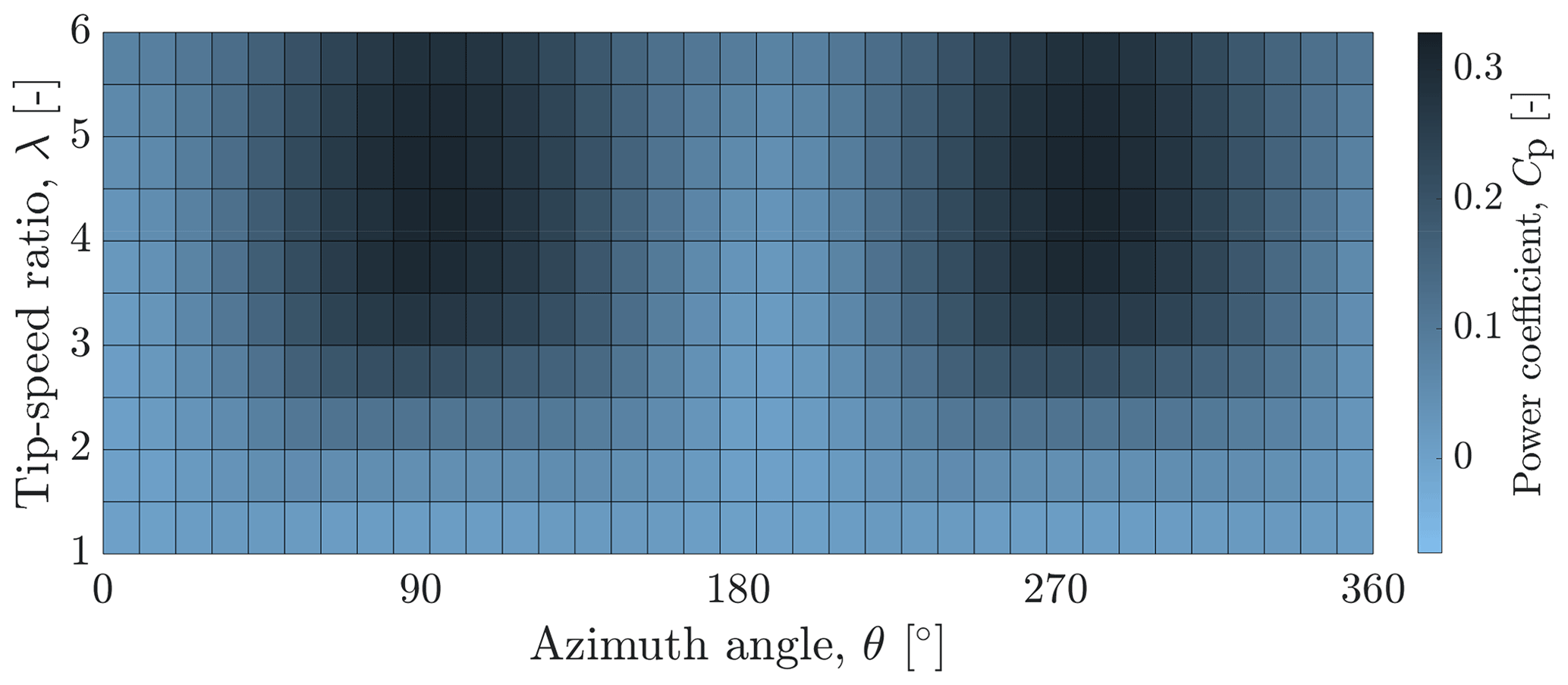
Figure 2Power coefficient Cp, as a function of the tip-speed ratio λ and azimuth angle θ, for the two-bladed H-Darrieus VAWT. The maximum values for the Cp are observed at θ=90° and θ=270°, as they correspond to the most upwind locations for blade 1 and blade 2, respectively. Due to the presence of these two blades, the twice-per-revolution (2P) periodicity of Cp is evident, especially at high values of λ.
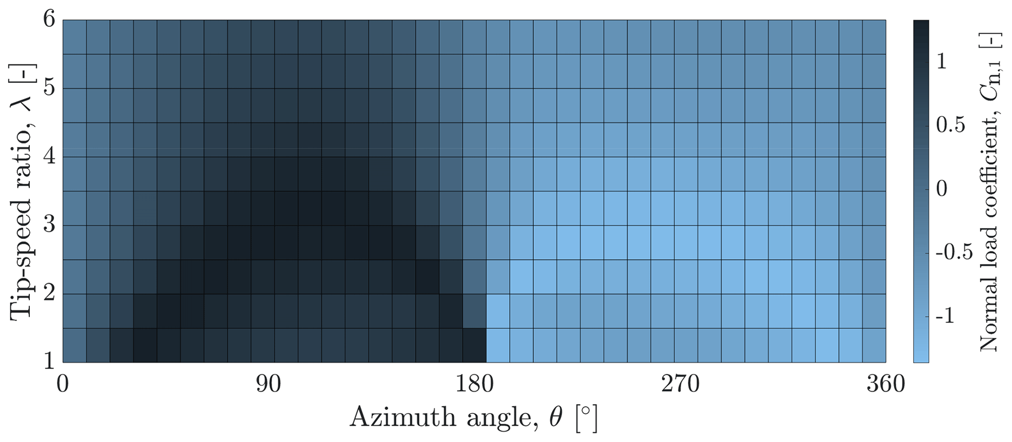
Figure 3Normal load coefficient mapping Cn,1, as a function of the tip-speed ratio λ and azimuth angle θ, for blade 1 of the H-Darrieus VAWT. It is evident that the normal blade force varies over the rotation, being positive upwind () and negative downwind (), with its maximum value at an azimuth angle θ=90°. These dynamics demonstrate the presence of a once-per-revolution periodicity (1P) on the Cn,1.
The wind turbine can be linearised around a specific operating point with the definition of the rotor and blade dynamics at hand. Firstly, the non-linear formulation of the aerodynamic rotor torque from Eq. (4) is combined with Eq. (2). The resultant expression is then linearised concerning the rotor speed state, wind speed disturbance input, and generator torque control input. The outcome is represented by
The original variables express the values perturbed around their operating points to ensure conciseness, while G(V),H(V), and E represent partial derivatives defined as
The variable V is introduced to conveniently define estimator-based expressions for G and H in a subsequent section, but it is excluded in the following terms.
The time-domain form of Eq. (7) is then Laplace transformed to give the transfer functions from wind speed and generator torque inputs to rotor speed as output:
where s represents the Laplace operator. The variables Ωr,𝒱, and 𝒯g indicate the frequency-domain representation of the rotational speed, wind speed, and generator torque, respectively.
The Kω2 controller is an effective and widely used approach for maximising energy capture in partial-load operation. However, the control strategy is limited in balancing power and actuation effort objectives for large-scale wind turbines. To address this issue, the more advanced WSE–TSR tracking scheme offers greater control flexibility. The current study aims to evaluate these findings for small-scale wind turbines, particularly VAWTs, which are promising solutions for urban environments.
This section derives the complete and non-linear representations of both the WSE–TSR tracking controller and the baseline Kω2 used for comparison. This process involves identifying the essential component building blocks for each scheme. Subsequently, a linear frequency-domain framework is formulated to analyse the controllers and closed-loop systems. This framework was derived in Brandetti et al. (2023b), and the main results are given here; the interested reader is referred to the referenced work for a detailed derivation. The subscripts (⋅)K and (⋅)TSR differentiate between the transfer functions for the Kω2 and WSE–TSR control schemes, respectively.
The two torque control strategies applied to the VAWT are formalised in the following based on the defined wind turbine dynamics. First, the complete and non-linear formulation of the Kω2 controller is obtained, followed by the derivation of the WSE–TSR tracking controller. An overview of the control frameworks is provided in Fig. 4 to facilitate the comparison between the two schemes. As can be observed, both controllers aim to maximise the power production of the urban VAWT by using the reference tip-speed ratio λ* and the measured rotor speed ωr as inputs. A more detailed description of each block diagram is given in the sub-sections below.
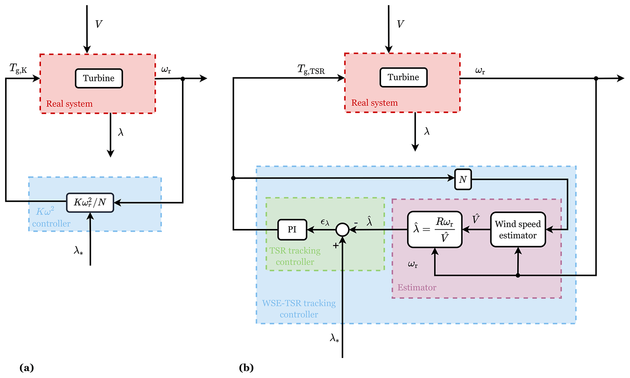
Figure 4Block diagram for (a) the Kω2 and (b) the WSE–TSR tracking control frameworks. In both schemes, the wind turbine system, highlighted in the red box, has two inputs (the wind speed, V, and the generator torque, Tg,K and Tg,TSR, respectively, if the Kω2 or the WSE–TSR tracking controller is applied) and two outputs (the tip-speed ratio, λ, and the rotational speed, ωr). In (a) the Kω2 block diagram, the controller (cyan box) uses the measured ωr and the optimal tip-speed ratio, λ*, as inputs to compute Tg,K. On the other hand, for (b) the WSE–TSR tracking controller, the cyan box encompasses the estimator (purple box) and the TSR tracker controller (green box). The estimator block applies the measured Tg,TSR and ωr to estimate the rotor-effective wind speed and to calculate an estimate of the tip-speed ratio, . The controller operates on the difference between and the optimal tip-speed ratio, λ*, to determine the torque control signal Tg,TSR.
3.1 Baseline Kω2 controller
The Kω2 controller is widely used for the operation of a small-scale VAWT. As Haque et al. (2008) demonstrated, this controller effectively maximises turbine power production by measuring the rotor speed and determining the reference torque. However, no comparison with a more advanced controller is provided. This study employs the Kω2 control law as a baseline, deriving the equations characterising its performance. The block diagram of the controller, shown in Fig. 4a, includes the wind turbine and the controller. It becomes evident that the controller operates as a static non-linear function, generating the control signal for the generator torque using the rotor speed. The control signal is given by
where the torque gain K (Bossanyi, 2000) is determined at the low-speed shaft side of the drivetrain as
The optimal power coefficient for maximum energy extraction and the associated optimal tip-speed ratio are and λ*, respectively.
3.2 WSE–TSR tracking controller
The WSE–TSR tracking control scheme illustrated in Fig. 4b comprises an estimator and a tip-speed ratio tracking controller and has been shown to optimise the turbine performance of VAWTs in turbulent wind conditions (Eriksson et al., 2008; Bonaccorso et al., 2011). The estimator employs the measured output of the real system, control signal, and a non-linear wind turbine model to compute an estimate of the REWS using the immersion and invariance (I&I) estimator (Ortega et al., 2013) with an augmented integral correction term (Liu et al., 2022). Assuming the measurement of the generator torque control input and the turbine's rotational speed and considering the REWS to be an unknown positive disturbance input to the plant, the formulation of the estimator is as follows:
where represents the estimated REWS; Kp,w and Ki,w are the proportional and integral estimator gains, respectively; t denotes the current time step; and τ is the integration variable. The estimated aerodynamic torque is defined as
with being the estimated power coefficient, a non-linear mapping of the estimated tip-speed ratio . Also, in this case, the pitch angle β is constant and equals 0°.
Then, the proportional and integral (PI) controller in the WSE–TSR tracking scheme operates on the difference between the estimated and reference tip-speed ratio λ*. The resulting error is utilised to determine Tg,TSR, being the generator torque demand, forcing the turbine to track the reference as
in which ϵλ is the tip-speed ratio error, Kp,c is the proportional controller gain, and Ki,c is the integral controller gain.
3.3 Analysis framework
The universal analysis framework proposed in Brandetti et al. (2023b) is used to evaluate the characteristics of the described control strategies and closed-loop systems. Only the main results are given in this section; the reader is referred to the referenced work for a more extensive derivation and explanation of the framework. The framework is depicted in Fig. 5, where the controllers are represented as one block with the rotor speed and the reference tip-speed ratio as inputs and the generator torque control signal as output. Each control scheme is formalised in the linear and frequency-domain formulation as
in which and represent the feedback and the reference shaping terms, respectively, and Λ* indicates the reference tip-speed ratio signal in the frequency domain.
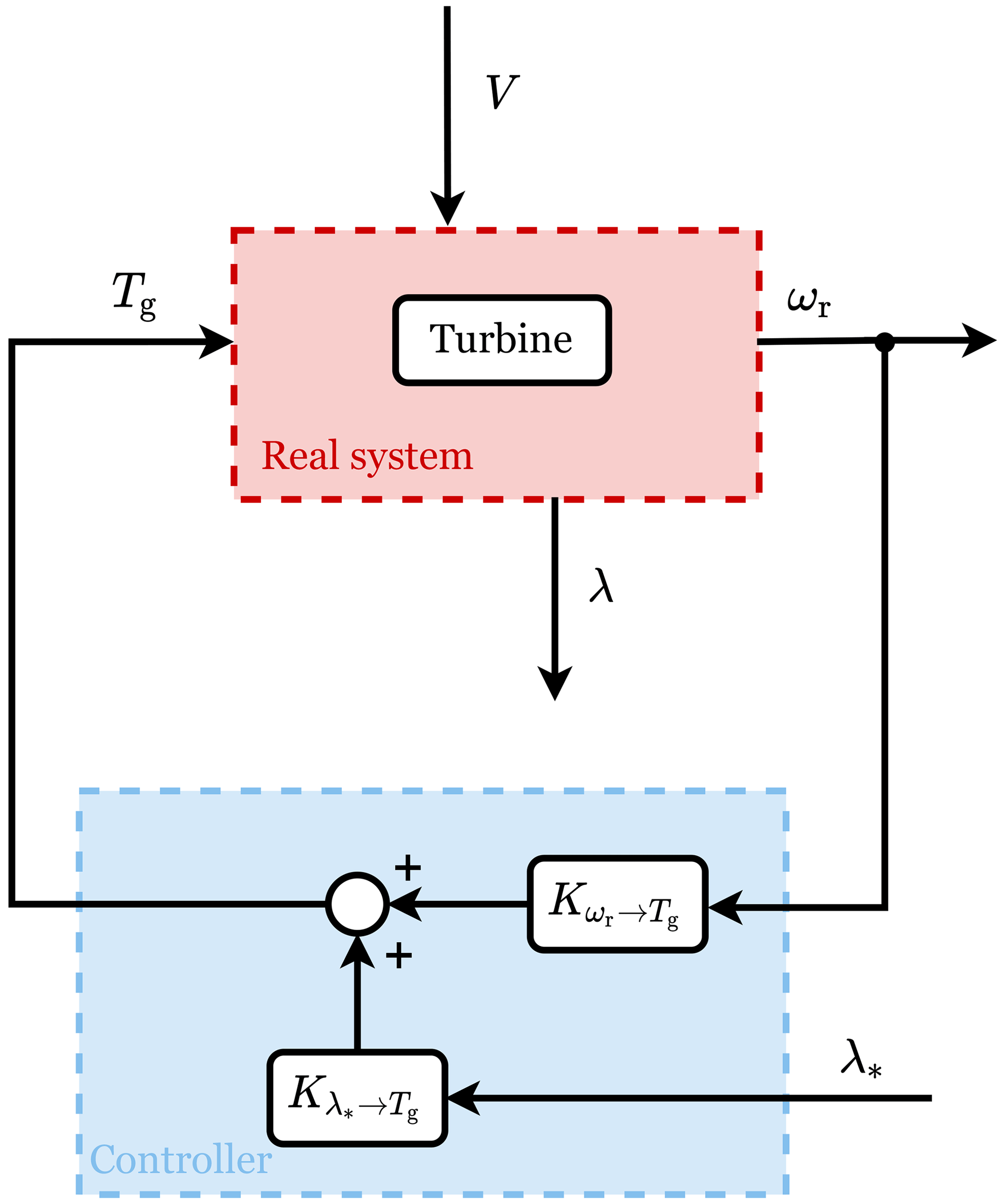
Figure 5Block diagram illustrating the universal framework employed for the controller analysis (Brandetti et al., 2023b). The wind turbine system is represented with the red box having the generator torque, Tg, and the wind speed, V, as inputs and the rotational speed, ωr, and the tip-speed ratio, λ, as outputs. The feedback term, , and the reference shaping term, , used in the analysis framework are included in the cyan box, symbolising the controller with two inputs (ωr and the tip-speed ratio set point, λ*) and one output (Tg).
Combining Eq. (16) with Eq. (10) and after manipulation, it is possible to derive the closed-loop transfer functions. As the scheme intends to regulate the tip-speed ratio to its reference value, the closed-loop transfer functions are expressed as a function of the turbine's actual tip-speed ratio λ. It follows that the two transfer functions representing the closed-loop system reference tracking and disturbance attenuation capabilities are defined as
Specifically, the term is the complementary sensitivity function, indicating the controller performance in tracking the commanded reference (i.e. ); the sensitivity function T𝒱→Λ(s) represents the controller performance in rejecting wind speed disturbances (Brandetti et al., 2023b). The represents values corresponding to a specific operating point in the analysis framework.
3.3.1 Baseline Kω2 controller
To determine the Kω2 controller dynamics, Eq. (11) can be linearised and combined with Eq. (10), representing the linearised wind turbine dynamics. It follows the feedback and the reference shaping terms defined according to the universal controller framework (Brandetti et al., 2023b) as
It can be observed from Eqs. (18) and (19) that the transfer functions of the controller are frequency-independent gains for the baseline controller.
3.3.2 WSE–TSR tracking controller
The WSE–TSR tracking controller dynamics are obtained through the initial linear derivation of the individual estimator and controller in the frequency domain. Subsequently, coupling between the estimator and the controller is performed to achieve the dynamics of the overall scheme. The interested reader is referred to Brandetti et al. (2023b) for the complete derivation. For conciseness, only the controller transfer functions are reported here as
and
characterising, on the one hand, the transfer function from the rotational speed to the generator torque output and, on the other hand, the transfer function from the tip-speed ratio reference to the generator torque output. To simplify Eqs. (20) and (21), the unspecified variables in the preceding formulations are denoted as
As the considered WSE–TSR tracking control scheme incorporates turbine model information that accurately reflects the characteristics of the wind turbine system without explicitly addressing inherent uncertainties present in real-world turbine dynamics, the variables and represent the estimated partial derivatives as formulated in Eqs. (8) and (9).
This section outlines the methodology for estimating the noise generated by the VAWT under investigation and assessing the subsequent expected psychoacoustic annoyance. Figure 6 shows the subsequent steps required to determine the psychoacoustic annoyance metric. First, the acoustic emissions of the VAWT are modelled using the noise prediction method, which was introduced and validated against high-fidelity simulations in Brandetti et al. (2023a). The estimated wind turbine noise spectra over time are then auralised to make the signal audible and then evaluated with a perception-based approach (Merino-Martínez et al., 2021) to determine the expected psychoacoustic annoyance.
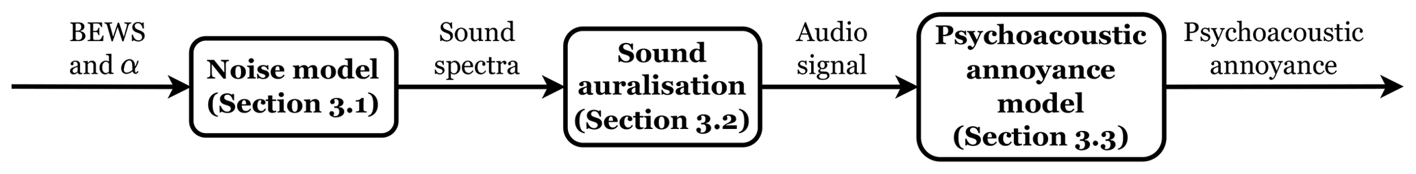
Figure 6Block diagram illustrating the integrated low-fidelity noise model and the psychoacoustic annoyance model based on perception-based psychoacoustic sound quality metrics. The first step is loading the blade-effective wind speed (BEWS) and the angle of attack (α), retrieved from the aero-servo-elastic simulations of the VAWT in QBlade (Marten, 2020), into the noise model. Then, the estimated sound spectra are auralised, generating realistic audio signals. These audio files are then evaluated using psychoacoustic sound quality metrics to estimate the psychoacoustic annoyance.
4.1 Noise prediction model
This section provides an overview of the model used to estimate the aeroacoustic performance of the VAWT. Interested readers are referred to Brandetti et al. (2023a) for more comprehensive details. The noise model exclusively accounts for aerodynamic sources, excluding any influence from mechanical or electrical components, as aerodynamic noise is deemed dominant for these turbines. The model evaluates three distinct aerodynamic noise generation mechanisms that are considered dominant for the two-bladed 1.5 m H-Darrieus VAWT:
-
laminar boundary layer–vortex shedding (LBL–VS) noise
-
turbulent boundary layer–trailing edge (TBL–TE) noise
-
turbulence–interaction (T–I) noise.
Among these sources, LBL–VS and TBL–TE are self-generated by the airfoil interacting with a steady flow (Brooks et al., 1989), whereas the T–I noise occurs from the interaction between the blade leading edge and inflow turbulence (Rogers et al., 2006; Kim et al., 2016). Note that the noise prediction model does not consider blade–blade interaction, as the blades are treated as isolated entities, and it assumes steady, free-stream conditions with quasi-steady time dependence.
The estimation of these noise sources involves several steps. Firstly, each blade is discretised in a three-dimensional space, dividing it into sequential strips. These strips possess identical airfoil chords and finite spans. Then, the computational domain is discretised in time, enabling the blade to progress along its rotational trajectory for a complete revolution (Botha et al., 2017). Consequently, for each blade element and azimuthal position, the airfoil self-noise and T–I noise are estimated using the methodologies presented by Brooks et al. (1989) and Buck et al. (2016), respectively. The relevant equations to implement these models are provided in Appendices A and B and rely on flow input parameters, including the angle of attack α and the BEWS. In the work conducted by Brandetti et al. (2023a), these parameters were estimated with the two-dimensional actuator cylinder model (Madsen, 1982). This study aims to enhance the accuracy of acoustic predictions by solving the flow over the blade using three-dimensional lifting-line free vortex wake simulations performed in the aero-servo-elastic software QBlade (Marten, 2020). After determining the sound pressure levels from these semi-empirical models, a Doppler correction factor is computed for the considered noise sources to account for the relative motion between the blade and the stationary observer (Ruijgrok, 1993). The total noise emissions along the blades and throughout a single rotation are finally calculated employing the approach Brooks and Burley (2004) developed.
The resulting sound pressure levels for the three noise sources are then used as inputs to perform the sound auralisation to make the signals audible and assessable with the perception-based approach to determine the corresponding psychoacoustic annoyance.
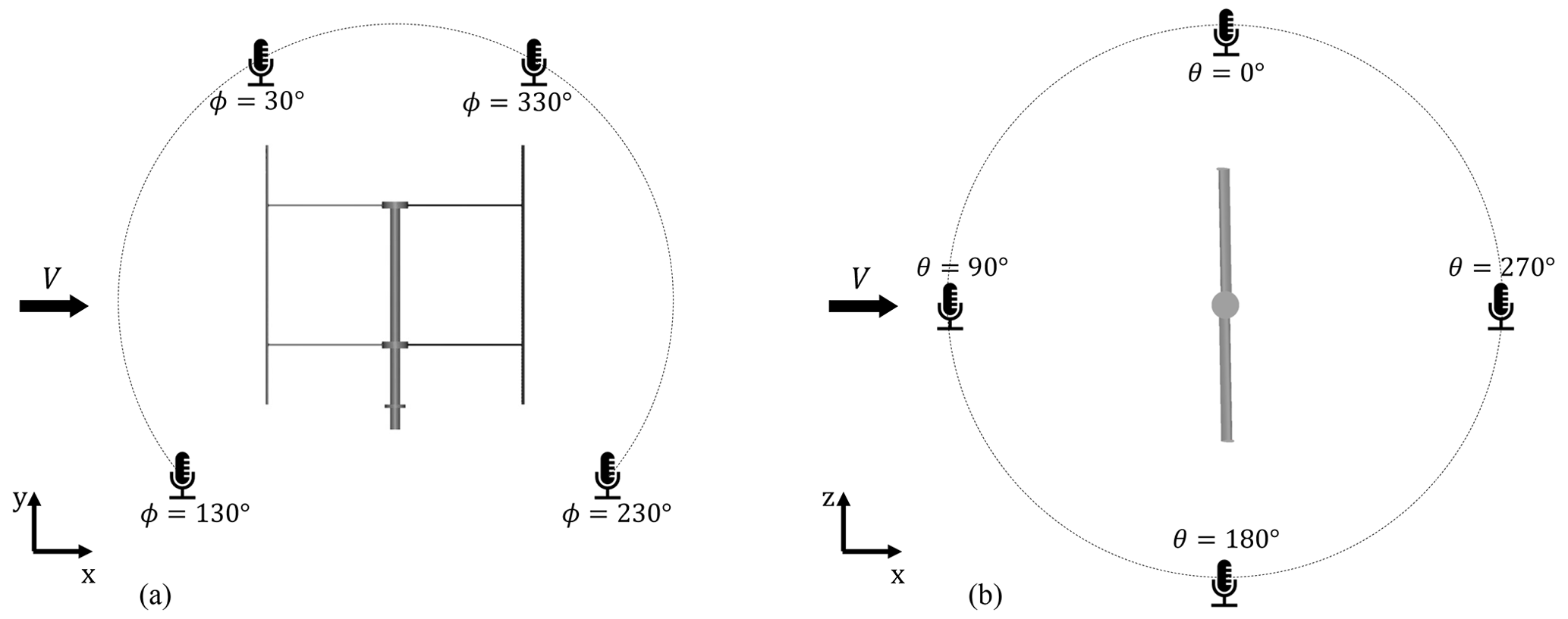
Figure 7Two circular arrays of virtual microphones are positioned at a distance of 2.6 D from the centre of the VAWT. Array (a) comprises four microphones located in the x–y plane, while array (b) consists of four microphones positioned in the x–z plane. These locations are considered relevant for characterising the psychoacoustic annoyance of the sound source.
4.1.1 Observer location
In the proposed low-fidelity noise model, eight virtual microphones are considered. As shown in Fig. 7, there are two circular arrays in the y–z and x–z planes, consisting of four virtual microphones, each positioned at 2.6D from the centre of the VAWT. This setup is chosen to cover the three-dimensional sound field of the turbine. The noise model is able to estimate the sound spectra at each of these observer locations. For every case study, a single observer location is chosen in the next section, describing the sound auralisation procedure.
4.2 Sound auralisation
The propagated sound spectra estimated in Sect. 4.1 are then auralised to obtain the audio signal in the time domain that a virtual observer at a specific location would perceive. Auralisation is a technique that enables artificially making an acoustic situation audible from numerical (simulated, measured, or synthesised) data (Vorländer, 2008). It can be considered the acoustic counterpart to visualisation.
To achieve more realistic auralised audio waves, each propagated one-third octave band spectrum per time step was interpolated to obtain an equivalent narrow-band spectrum with a frequency step of 1 Hz while maintaining the same sound pressure level per one-third octave band. This practice is common when auralizing the output of noise prediction models, which typically provide outputs as one-third octave band spectra (Pieren et al., 2019; Maillard et al., 2023). The narrow-band spectrum corresponding to each time block is then converted to the time domain using an inverse short-time Fourier transform, following the guidelines explained in Vorländer (2008) and Merino-Martínez et al. (2021). Each time block was windowed using a Hanning weighting function with 50 % data overlap. A similar approach has recently been applied to the auralisation of HAWT noise (Pieren et al., 2014; Maillard et al., 2023). The interested reader is referred to the aforementioned publications for a more detailed explanation.
The resulting audio files were then fed into the psychoacoustic annoyance model (see Sect. 4.3) to estimate the psychoacoustic annoyance of each sound, which is described in the next section.
4.3 Psychoacoustic annoyance model
This section introduces the psychoacoustic annoyance model employed for estimating the perceived annoyance due to the noise emitted by a VAWT in an urban environment. The audio files determined with the auralisation of the sound spectra in Sect. 4.2 are assessed using a combination of perception-based sound quality metrics (SQMs) (Fastl and Zwicker, 2007; Di et al., 2016) to estimate the psychoacoustic annoyance.
Unlike the SPL metric, which quantifies the purely physical magnitude of sound based on the measured acoustic pressure, SQMs describe the subjective perception of sound by human hearing. Therefore, these metrics have been shown to better capture the auditory behaviour of the human ear compared to the conventional sound metrics typically employed in wind turbine noise assessments (Merino-Martínez et al., 2021, 2022). The psychoacoustic annoyance model considers the five most common SQMs (Greco et al., 2023a):
-
Loudness (𝒩). This is the subjective perception of sound magnitude corresponding to the overall sound intensity. The model proposed by the International Organization for Standardization (2017) and standardised in the ISO 532-1 norm was employed in this work. The unit of this metric is the sone (on a linear scale) or the phone (on a logarithmic scale).
-
Tonality (𝒦). This is the measurement of the perceived strength of unmasked tonal energy within a complex sound following the model by Aures (1985). This metric is measured in tonality units (t.u.) and its values range from 0 (purely broadband) to 1 t.u. (purely tonal).
-
Sharpness (𝒮). This is a representation of the high-frequency sound content (especially frequencies higher than 3000 Hz), as described by von Bismarck (1974) and the German norm DIN 45692:2009. The unit of this metric is the acum.
-
Roughness (ℛ). This is the hearing sensation caused by sounds with fast amplitude modulations with modulation frequencies between 15 and 300 Hz. The model by Daniel and Webber (1997) was considered in this study, and the unit of this metric is the asper.
-
Fluctuation strength (ℱs). This is an assessment of slow fluctuations in loudness with modulation frequencies up to 20 Hz, with maximum sensitivity for modulation frequencies around 4 Hz. This work employs the model proposed by Osses Vecchi et al. (2016). The unit of this metric is the vacil.
All SQMs were computed using the open-source MATLAB sound quality analysis toolbox (SQAT) (Greco et al., 2023b), and the 5 % percentiles were considered, representing the threshold value of each SQM that is exceeded for 5 % of the total signal time. Following the formulation of Di et al. (2016), these SQMs can be combined to compute the psychoacoustic annoyance (PA) as
The variables υ𝒮(𝒩,𝒮), υ𝒦(𝒩,𝒦), and denote the contributions of the sharpness, tonality, roughness, and fluctuation strength, respectively. As can be observed, the loudness contribution is considered in all three terms as it exerts the strongest influence on psychoacoustic annoyance. For the sake of conciseness, the formulation for these three terms is omitted, but the interested reader is referred to Di et al. (2016) and Fastl and Zwicker (2007) for additional information on the field of psychoacoustics and to Greco et al. (2023b, a) for the implementation of the SQMs considered.
This section presents the architecture for implementing and optimally calibrating torque control strategies in small-scale VAWTs using the mid-fidelity wind turbine simulation software QBlade (Marten, 2020).
In the following, Sect. 5.1 formally defines the multi-objective optimisation problem. Section 5.2 explains the multi-criteria decision-making method selected to find the trade-off on the resulting Pareto front. Section 5.3 describes its implementation as a systematic search and guided exploration of the calibration variables for the considered controller, aiming to assess the performance space across all objectives.
5.1 Multi-objective optimisation
The present study investigates a multi-objective optimisation problem characterised by a cluster of continuous input variables 𝒳⊂ℝd, referred to as the design space (Lukovic et al., 2020). The objective is to minimise an objective function vector, denoted as , where m≥2. In this context, x∈𝒳 represents the input variable vector, and f(𝒳)⊂ℝm denotes the m-dimensional image representing the performance space. Thus, the objective is to solve the following minimisation problem, subject to the operating conditions governing the multi-objective optimisation process:
Since there is an inherent conflict among the objective functions, a single optimal solution may not always exist. Instead, it is necessary to identify optimal solutions, known as the Pareto set 𝒫s⊆𝒳 in the design space and the Pareto front in the performance space (Lukovic et al., 2020). In this study, the Pareto front is approximated by considering a point , as Pareto is optimal if there is no other point x∈𝒳 such that for all j and for at least one j, where (Miettinen, 1999).
5.2 Multi-criteria decision-making method
From the description of the multi-objective optimisation, it is clear that all points within the Pareto front represent equally optimal solutions. No solution is better than others in satisfying all conflicting objectives, as enhancing objective function inevitably compromises others (Gambier, 2022; Lara et al., 2023a, b). Once the Pareto front is approximated, the decision-maker can assess various options and select the most favourable one. This collection of potential solutions underscores the adaptability of the design-making process, wherein the designer's role is to identify the optimal solution tailored to specific circumstances (Santín et al., 2017).
To facilitate the decision-making stage, this paper aims to provide designers with a solution to the optimal calibration of the WSE–TSR tracking controller. Therefore, a multi-criteria decision-making (MCDM) method is proposed to select an appropriate trade-off of the considered objective functions. An MCDM method typically involves p alternatives () and q criteria () , structured as a decision matrix and weight vector , in which yc,k is the performance of the cth alternative with respect to the kth criterion, and wk is the weight of the kth criterion (Wang et al., 2016).
Simple additive weighting (SAW) is applied to each point along the Pareto front, as it is considered the most intuitive and straightforward MCDM approach (Afshari et al., 2010; Bagočius et al., 2014). In the SAW method, the final score of a candidate solution is determined by summing the weighted values of its attributes, accomplished through three sequential steps (Wang et al., 2016). Firstly, the decision matrix Y is normalised to enable fair comparison across the different criteria, using the sum method, which is widely applied in the literature (Lee and Chang, 2018). This normalisation yields the normalised decision matrix . Subsequently, weight values are assigned to each criterion Cq within the weight vector W (Wang et al., 2016). The next step involves the calculation of the ranking score Sc for each alternative as
The alternative with the highest Sc value is considered the most satisfactory solution (Lara et al., 2023a), and the associated calibration parameters are deemed the most effective trade-off settings for calibrating the WSE–TSR tracking controller.
5.3 Implementation of the controller and optimisation framework
In this section, first, the objective functions employed for the multi-objective optimisation of the WSE–TSR tracking controller are defined, followed by a detailed description of the simulation implementation.
5.3.1 Definition of the objective function
The approach employed to calibrate the design variables of the WSE–TSR tracking control scheme conforms to the previously described multi-objective optimisation problem and MCDM method. In this case, a three-dimensional vector captures the objective functions and is expressed as follows:
The first objective, f1(Γd), relates to the variance of the torque control signal, representing the controller's reactivity and serving as an indicator of the actuation effort on the turbine. This is defined as
The second objective, f2(Γd), encompasses the mean of the wind-turbine-generated power and is defined as
Note that the negative sign preceding the power term is inherent in the context of the minimisation problem defined in the multi-objective optimisation (Eq. 23).
The third objective, f3(Γd), concerns psychoacoustic annoyance, quantifying the perceived noise emitted by the wind turbine as
These objectives are expected to be conflicting in the sense that a highly responsive controller tends to increase power generation, actuation effort, and noise annoyance. Conversely, a more conservative controller calibration would decrease power production while being beneficial regarding the actuation and noise objectives.
In the aforementioned equations, the variables are defined as follows: L denotes the entire dataset size; represents the generator torque mean value; Tg,l and Pg,l indicate individual values of generator torque and power within the recorded data, respectively; and PA is the psychoacoustic annoyance computed using α and BEWS.
It is evident that the resulting signals Tg, Pg, and PA are dependent on , which corresponds to the d-dimensional input variable vector. The current study investigates the input vector dimensionality to evaluate the controller performance under two levels of complexity. The considered input vectors are denoted as
where the subscript (⋅)d indicates the dimension of each design space and is used to differentiate between the input vectors throughout the paper. It should be noted that the WSE–TSR tracking controller is originally formulated by setting d=5 and by denoting the corresponding calibration variables as . The selection of a subset from the original formulation is based on the findings reported by Brandetti et al. (2023b), where it is indicated that the inclusion of an integral term in the estimator (i.e. Ki,w) leads to minimal or no enhancement in the operation of the WSE–TSR tracking control scheme. On the other hand, Γ1 represents the Kω2 controller design space being one-dimensional as the variation in λ* results in corresponding changes in the gain K, described in Eq. (12).
5.3.2 Simulation implementation
Figure 8 provides an overview of the overall implementation and optimal controller calibration, which enables the execution of various simulations to explore the parameter space of the considered controllers through a guided search procedure. This process yields a set of optimal solutions that form the Pareto fronts, representing a trade-off between f1(Γd), f2(Γd), and f3(Γd). The workflow consists of several steps. First, the input parameters, such as the turbine geometry, operating conditions, and torque control strategy, are defined. Then, mid-fidelity simulations are conducted employing the aero-servo-elastic software QBlade (Marten, 2020), loaded as a dynamic link library in MATLAB; the interested reader is referred to the tutorial by Brandetti and van den Berg (2023) for further details about this interface and to Appendix C for a detailed description of the QBlade turbine model. This interface allows for the parallelisation of the original simulation case, referred to as ORIGIN in Fig. 8, up to a specified index t=T, significantly reducing the computational time for the multi-objective controller optimisation. Per simulation, t, the controller settings are randomly varied and adhere to the constraints imposed by the design space. In this way, a range of optimal solutions is explored through a guided search within the constrained design space approximating the Pareto front .
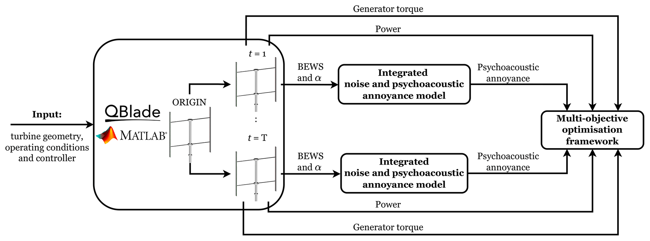
Figure 8Block diagram illustrating the implementation and optimal calibration of controllers applied to the two-bladed 1.5 m H-Darrieus VAWT. The process involves the following: defining input parameters, parallelising the ORIGIN simulation case in cases, running simulation t with varied controller gains, extracting aero-servo-elastic information, loading the blade-effective wind speed (BEWS) and the angle of attack (α) into the integrated noise and psychoacoustic annoyance model to retrieve the corresponding psychoacoustic annoyance, and using the information within a multi-objective optimisation framework to determine the optimal calibration for the selected controller.
The VAWT operates in a turbulent wind profile characterised by a mean wind speed of m s−1 and a turbulence intensity of 15 %. The simulation is set over a specific duration; however, for the analysis, only an average of 680 complete turbine revolutions is considered to eliminate any transient start-up effects from influencing the results. Subsequently, the obtained time series data are used to calculate f1(Γd) and f2(Γd).
For the computation of the third objective (noise annoyance), α and BEWS are extracted from these time series and employed as inputs for the noise prediction model (Sect. 4.1). The SPLs for the three noise generation mechanisms described in Sect. 4.1 are calculated for each time step within one full blade revolution period. Due to the different rotational speeds considered, the rotational period was different for different operational conditions. To consider the total noise emissions of the VAWT, the contributions of the three noise generation mechanisms (LBL–VS, TBL–TE, and T–I) were summed logarithmically for every time step and propagated to the selected observer position. The resulting sound spectra are then auralised, as explained in Sect. 4.2, to achieve realistic audio files, which are fed into the psychoacoustic annoyance model (Sect. 4.3), determining f3(Γd). Note that for the considered case study, it was found that ℛ and ℱs did not vary significantly. Therefore, a modified version of the PA model, employed in Merino-Martínez et al. (2022), is applied where these two metrics are not considered, equivalent to setting υℱℛ=0. In the following, f3(Γd) is defined as PAmod to denote the modified version.
The last step is to use the computed objective functions f1(Γd), f2(Γd), and f3(Γd) within the multi-objective optimisation framework to determine the optimal calibration for the considered controller.
This section presents the multi-objective optimisation results. The exploration of the performance space is conducted through a guided search procedure for the group of design variables Γ1 and Γ4, corresponding to the Kω2 controller and the WSE–TSR tracking controller, respectively. The approximation of the Pareto fronts is based on the minimisation of a weighted linear combination of the objectives f1(Γd), f2(Γd), and f3(Γd), leveraging the data obtained during the exploration process.
The MCDM approach provides a trade-off between the considered objectives, leading to the optimal calibration for both the WSE–TSR tracking controller and the Kω2 controller. Subsequently, a comparative analysis of the resulting optimal controllers is conducted from two distinct perspectives: the wind turbine performance and the controller performance. Regarding the former perspective, time-domain results are used to evaluate the turbine from an aero-servo-elastic point of view. Additionally, the sound spectra averaged over a rotation are presented in the frequency domain to characterise the acoustic emissions of the VAWT in an urban environment. By extending the analysis beyond conventional performance metrics like power and torque, this study emphasises the critical importance of addressing the impact of noise emissions on psychoacoustic annoyance and its subsequent influence on public perception of VAWTs in urban environments. Lastly, the section uses the frequency-domain framework outlined in Sect. 3.3 to draw conclusions about controller bandwidth and disturbance rejection performance.
Notably, the analysis focused exclusively on the results obtained from the microphone at θ=90°, as Brandetti et al. (2023a) demonstrated the VAWT's almost-omnidirectional behaviour in terms of overall sound pressure level when averaging all noise sources.
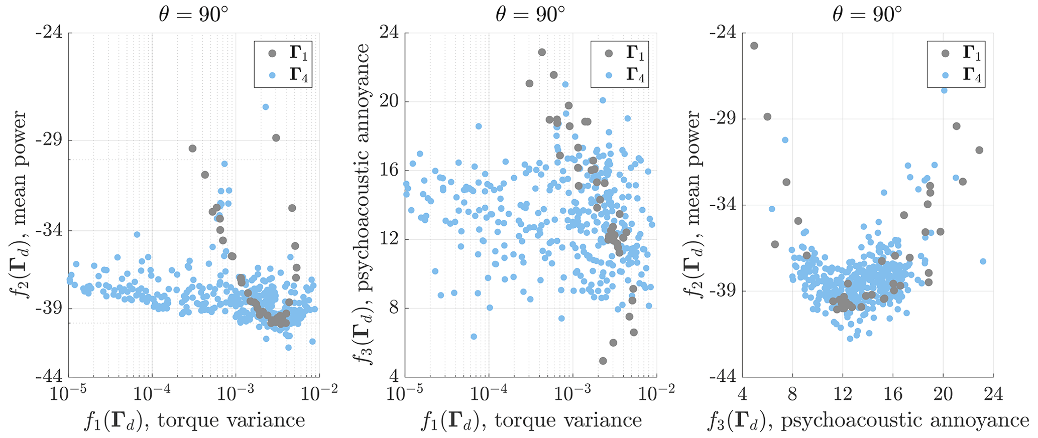
Figure 9Results of the WSE–TSR tracking control scheme's performance in turbulent wind conditions attained by an exploratory search of two estimator-controller calibration variables: Γ1 and Γ4. The controller performance space is defined by the three objective functions f(Γd). For the calculation of the psychoacoustic annoyance, the microphone in the x–z plane at θ=90° is selected.
6.1 Pareto front and case study definitions
The Pareto front construction begins with systematically exploring the performance space, guided by an investigation of the input variables Γ. Figure 9 visually presents the data points obtained from the mid-fidelity simulation scenario. For the higher-dimensional design space Γ4, a more extensive dataset is collected to reconstruct the performance space of the WSE–TSR tracking controller. To facilitate comparative analysis, the Kω2 controller is used as a benchmark.
Significantly, within the Γ1 set, data points demonstrate a clustering pattern with a convex configuration, revealing a distinct global minimum for the objective functions f1(Γd) and f2(Γd). However, when f1(Γd) and f3(Γd) are considered to be objectives, a different pattern emerges. It becomes apparent that the psychoacoustic annoyance does not show a discernible trend with the torque variance, acting as a proxy for the controller actuation effort. Conversely, a clear correlation is observed between psychoacoustic annoyance and mean power production for both the Γ1 and the Γ4 sets, indicating that higher power extraction levels do not necessarily lead to increased psychoacoustic annoyance.
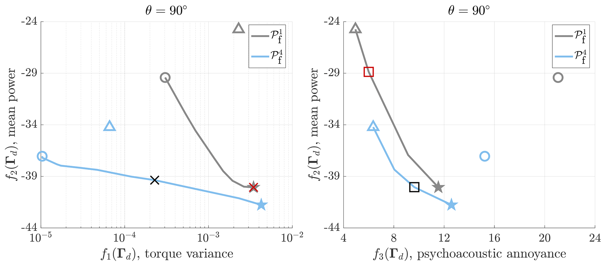
Figure 10Pareto fronts and derived for the Kω2 and the WSE–TSR tracking controllers under turbulent wind conditions, respectively. For the calculation of the psychoacoustic annoyance, the microphone θ=90° is selected in the x–z plane. The optimal solutions for f1(Γd), f2(Γd), and f3(Γd) are indicated using circles (◦), stars (⋆), and triangles (△), respectively. The trade-off solutions for the two controllers are shown with a cross (×) when f1(Γd) and f2(Γd) are considered to be objectives and with a square (□) when f2(Γd) and f3(Γd) are considered. In contrast to the baseline controller, the WSE–TSR tracking controller achieves improved power maximisation while reducing torque fluctuations and psychoacoustic annoyance, albeit with a slight compromise on power extraction.
From the available exploration data, the Pareto front is estimated. Figure 10 illustrates the derived Pareto fronts ( and ) for two distinct dimensionalities of the input vector Γd, facilitating a comparative analysis between the baseline and the WSE–TSR tracking controller performance, respectively. The circles (◦), stars (⋆), and triangles (△) in the plot represent the optimal solutions corresponding to each objective function, namely f1(Γd), f2(Γd), and f3(Γd), respectively. Based on the above-mentioned consideration, no Pareto front is constructed between f1(Γd) and f3(Γd) as the exploration points violate the Pareto optimality definition, described in Sect. 5.1. The trade-offs between f1(Γd) and f2(Γd) and f2(Γd) and f3(Γd) are computed applying the MCDM method defined in Sect. 5.2 and indicated with crosses (×) and squares (□), respectively.
The figure depicts that the higher-dimensional controller front (d=4) covers the performance space the most extensively, confirming the effectiveness of the WSE–TSR tracking control scheme in improving the Pareto optimal solutions. Specifically, the controller is capable of minimising psychoacoustic annoyance and torque fluctuations while exerting minimal influence on power extraction performance. In addition, the application of the WSE–TSR tracking controller to small-scale wind turbines, such as VAWTs in urban environments, leads to attainable power gains. The role of wind turbine inertia in the controller performance is evident, as a higher parameter value enhances resilience against deviations from the optimal operating point, causing no improvement in power production when applied to large-scale wind turbines (Brandetti et al., 2023b). However, the observed improved power production for the VAWT under study may result in a lower bandwidth than the baseline controller. This aspect will be investigated in the following by applying the frequency-domain framework described in Sect. 3.3.
The data derived from the Pareto front reveal key insights, as presented in Table 2. This table provides a comprehensive quantitative analysis of the impact of optimal calibration points on system parameters. Specifically, the percentage increase is computed for each objective function, showcasing the change in the WSE–TSR tracking controller concerning the baseline Kω2. When comparing the optimal solution ◦, the WSE–TSR tracking controller demonstrates a remarkable reduction in actuation effort, up to 97 %. This reduction corresponds to a power production increase of 26 % and a psychoacoustic annoyance decrease of 28 %. As observed, the optimal solution △ also facilitates a reduction in torque fluctuations of up to 97 %, accompanied by a 38 % increase in mean power and a 28 % increase in psychoacoustic annoyance compared to the baseline.
Table 2Quantitative assessments of the Kω2 (Γ1) and the WSE–TSR tracking control scheme (Γ4) for different optimal solutions: ◦, ⋆, △, ×, and □. The percentage increase is computed for each objective function to show the percentage change in the WSE–TSR tracking controller with respect to the baseline Kω2. Optimal solutions, such as ◦ and △, demonstrate a substantial reduction in actuation effort alongside increased power production and psychoacoustic changes. However, in some cases like ⋆, the controller impact on f2(Γd) and f3(Γd) remains small. At the same time, trade-off solutions × and □ exhibit interplayed effects on various performance metrics, emphasising the multi-faceted nature of controller optimisation.
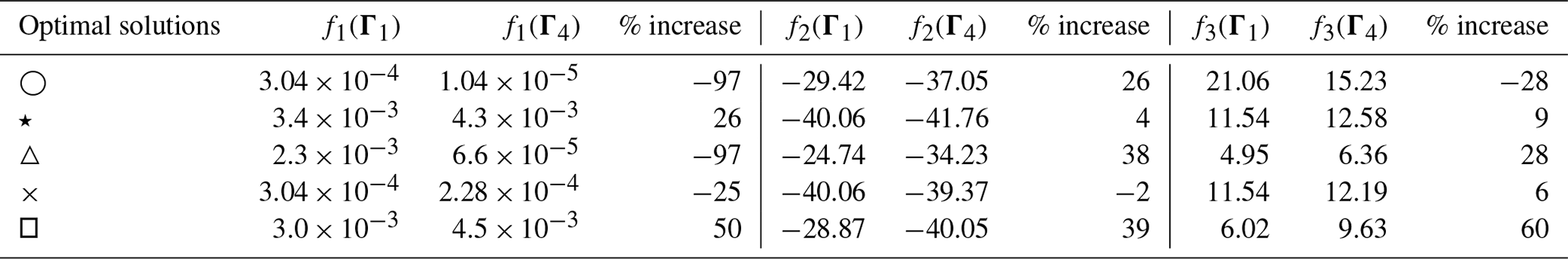
On the other hand, in the case of ⋆, the WSE–TSR tracking controller only marginally increases power production by 4 %, with a significant increase of 26 % in the torque variance and 9 % in the psychoacoustic annoyance. A closer examination of the trade-off optimal solution × indicates that the WSE–TSR tracking controller reduces actuation effort by 25 %, with a minor impact on power production (only a 2 % decrease) and psychoacoustic annoyance (only a 6 % increase). Conversely, for the □ case, the significant 39 % increase in power production is offset by an increase in the psychoacoustic annoyance of 60 % and an increase in torque fluctuations of 50 %. The results for the trade-off solutions highlight the complexities of the WSE–TSR tracking controller optimisation.
The following analysis only focuses on the trade-off results × and □ derived from the MCDM approach for the Kω2 and WSE–TSR tracking controllers. This selective approach aids the decision-making process by providing a clear representation of how these optimal solutions affect wind turbine and controller performance, offering calibration guidelines for the WSE–TSR tracking control scheme.
6.2 Wind turbine results
This section validates the insights obtained from the exploratory search and Pareto fronts by presenting the wind turbine performance results, focusing on aero-servo-elastic performance and acoustic emissions.
6.2.1 Aero-servo-elastic performance
The mid-fidelity simulations are conducted in QBlade using the VAWT turbine, as outlined in Sect. 2, under turbulent wind conditions for an urban environment, with a mean wind speed of m s−1, a turbulence intensity of 15 %, and a total simulation duration of 800 s. Figure 11 provides a comprehensive representation of the simulation results, encompassing the operating wind speed, tip-speed ratio, generator torque, generator power, tip-speed ratio tracking error, and rotor speed. A condensed representation of the results is included to highlight essential characteristics in the time-domain analysis.
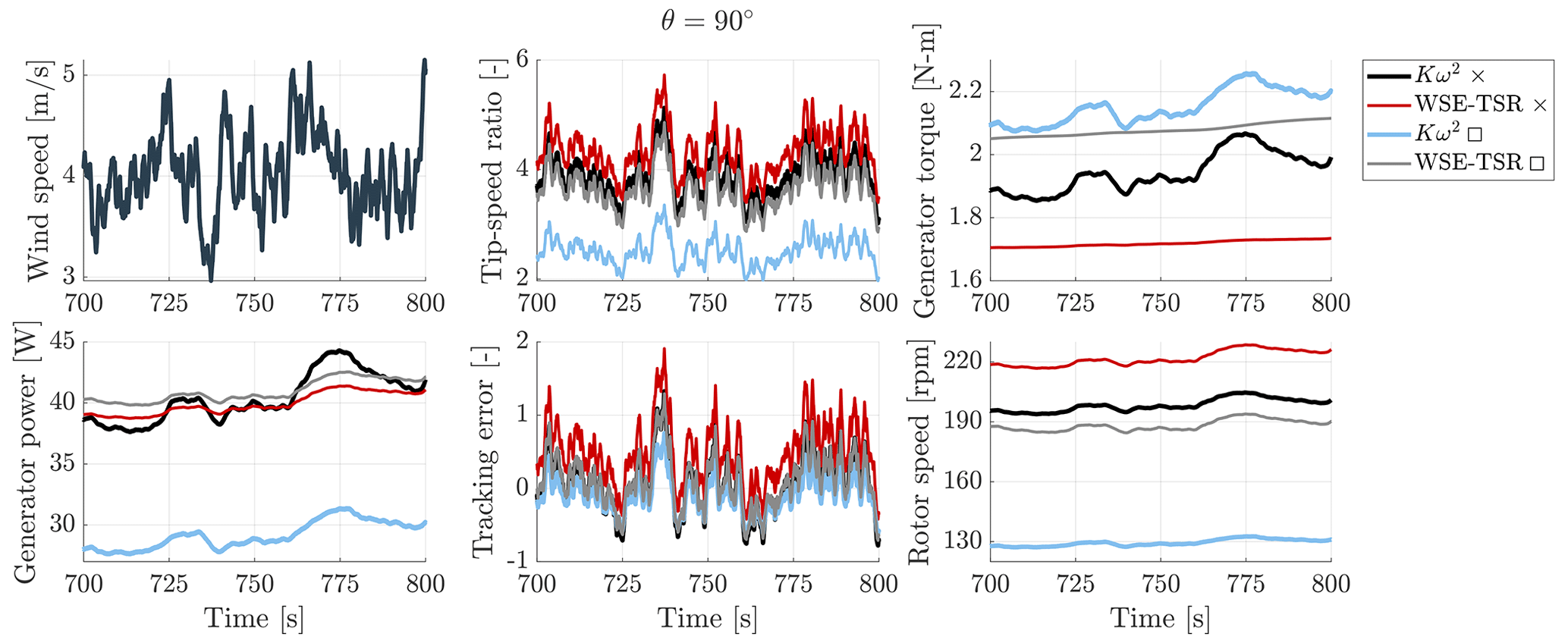
Figure 11Simulation results for the Kω2 and WSE–TSR tracking control schemes subject to a turbulent wind speed with a mean of 4 m s−1 and a turbulence intensity of 15 %. The WSE–TSR tracking controller demonstrates smoother generator curves compared to the fluctuating behaviour of the Kω2 controller. The Kω2 trade-off □ case displays a 25 % mean power reduction due to suboptimal operation at a reference tip-speed ratio . Overall, the WSE–TSR tracking controller achieves an optimal balance between reducing psychoacoustic annoyance and maintaining a power output comparable to the maximum power extraction of the baseline control scheme.
For both of the selected trade-off case studies of the WSE–TSR tracking controller, the simulations reveal smoother generator torque curves, demonstrating remarkable stability even under turbulent wind conditions. Conversely, the Kω2 controller exhibits sporadic fluctuations in the generator torque, potentially causing elevated actuation effort and compromising the turbine integrity over prolonged periods of operation. In particular, the trade-off □ case for the Kω2 controller exhibits a lower mean power than the other three cases, indicating a reduction of over 25 %. This difference arises from the controller operating at a non-optimal reference tip-speed ratio λ* of 2.6 for the power production of the studied VAWT, as illustrated in the power curve of Fig. 2. Consequently, the WSE–TSR tracking controller achieves a superior balance between minimising psychoacoustic annoyance and maximising mean production power, enabling comparable power output to the baseline calibrated for maximum power extraction while simultaneously reducing noise levels.
6.2.2 Acoustic emissions
The following investigation outlines the different noise generation mechanisms characterising a VAWT in an urban environment by comparing the selected optimal trade-off solutions for the WSE–TSR tracking controller against the baseline control scheme. Given that the psychoacoustic annoyance yields a numerical output, the analysis of noise spectra averaged over a rotation aids in establishing a link between psychoacoustic annoyance and the conventional sound pressure level, thereby effectively characterising the acoustic emissions of a VAWT. In particular, the A-weighted sound pressure level (SPLA) is employed to account for the relative loudness perceived by human hearing, albeit acknowledging that the insights provided are general and highly averaged (Merino-Martínez et al., 2021). The SPLA is measured in dBA and computed with the noise model of Sect. 4.1 at a radial distance of 2.6 D from the centre of the VAWT in the x–z plane, specifically at θ=90°.
By looking at the different SPLA spectra in Fig. 12 for the considered trade-offs, it is clear that the most dominant noise source is the T–I noise. The SPLA spectra further support the previous observations derived from the exploratory search and the construction of the Pareto front. Specifically, for the × case, the minimal difference in psychoacoustic annoyance is recognised in almost-overlapping spectra. Conversely, in the ⋆ case, the optimal WSE–TSR tracking controller shows higher psychoacoustic annoyance, reflected in higher SPLA levels across all three sources. For both cases, the differences between the controllers are most pronounced for the LBL–VS noise source. This is because the controllers lead to different trends in the angle of attack assumed by the wind turbine, which then leads to different alpha-dependent functions (Eq. A1) employed in the noise model to estimate this source.
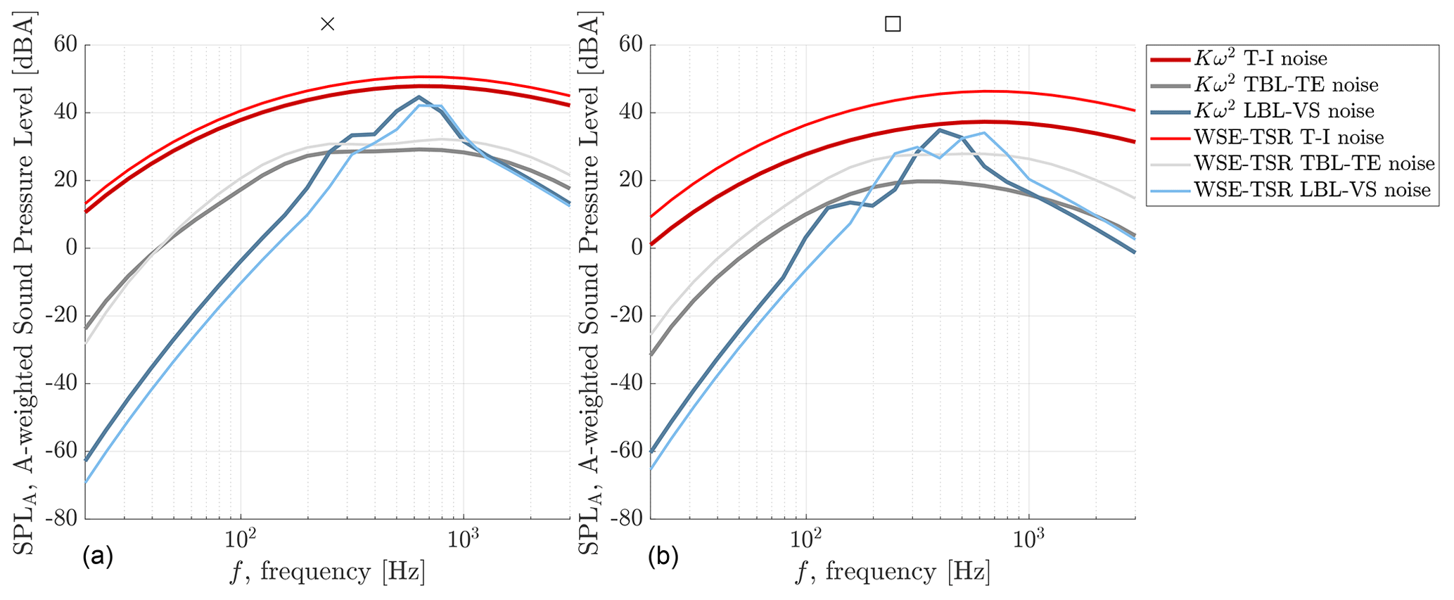
Figure 12A-weighted sound pressure level (SPLA) versus frequency (f) obtained from a microphone in the x–z plane at θ=90°. The Kω2 controller and the WSE–TSR tracking controller are calibrated to obtain a trade-off between mean power and torque variance, × (a), and a trade-off between mean power and psychoacoustic annoyance, □ (b). Overall, the most dominant noise source is the T–I noise.
6.3 Analysis of the controller performance
The current section presents the frequency-domain characteristics of the designated cases, employing the linear analysis framework defined in Sect. 3.3 (Brandetti et al., 2023b). The analysis presents the frequency responses of the transfer functions and T𝒱→Λ(s), indicating the performance of the closed-loop system in terms of reference tracking (complementary sensitivity) and disturbance rejection (sensitivity), respectively. Bode plots are illustrated in Fig. 13 for the MCDM solutions.
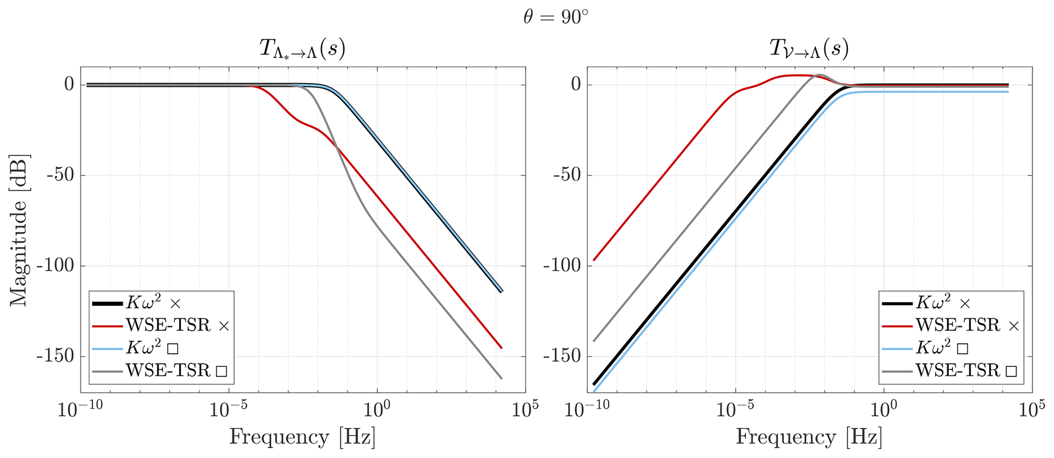
Figure 13Bode plots of the closed-loop transfer functions and T𝒱→Λ(s) for the baseline Kω2 and the WSE–TSR tracking controllers. The MCDM solutions for the WSE–TSR tracking controller reveal that the reference tip-speed ratio tracking and disturbance rejection capabilities have to be offset to achieve a 39 % increase in power production, for the × case, and a 25 % reduction in actuation effort, at the cost of 2 % power decrease and 6 % increase in psychoacoustic annoyance, for the □ case, compared to the Kω2 controller.
In the case of the trade-off Kω2 ×, the steady-state gain diverges with respect to the baseline gains due to the reference tip-speed ratio λ* calibrated at a lower and non-optimal value of 2.6. On the other hand, the two optimally calibrated WSE–TSR tracking controllers do not exhibit an improvement in control bandwidth but do demonstrate enhanced disturbance-rejection capabilities with respect to the baseline controller. This outcome aligns with the anticipated behaviour, as these optimal calibrations represent a balance between competing objectives, prioritising an integrated decision-making approach over mere power performance maximisation.
Furthermore, the results underscore the complex trade-offs inherent in the multi-objective calibration of the WSE–TSR tracking controller. As illustrated in Table 2, the improvements in reference tracking and disturbance rejection performance must be offset to achieve advancements in the considered performance metrics. For instance, the □ case demonstrates a remarkable 39 % increase in power production, while the × solution allows a significant 25 % reduction in torque actuation effort, albeit at the cost of a mere 2 % power decrease and a 6 % increase in psychoacoustic annoyance.
This study tackles crucial barriers to the acceptance of small-scale VAWTs in urban environments. Recognising the promising potential of VAWTs for urban wind energy generation, owing to their simple design, low maintenance costs, and reduced visual impact compared to HAWTs, the study emphasises the need to mitigate noise emissions to overcome local opposition. Specifically, the research explores the issue of noise annoyance, highlighting the need to incorporate psychoacoustic annoyance in the design and decision-making process to enhance community acceptance of VAWTs. Simultaneously, it underscores the importance of optimising VAWT torque control strategies to maximise the aero-servo-elastic performance of the turbine. By solving a multi-objective optimisation problem, an advanced control strategy is calibrated to achieve the trade-off between the considered operational performance and noise emissions.
In this study, the combined WSE–TSR tracking controller is employed, renowned for achieving flexible trade-offs in terms of power maximisation and load minimisation. This advanced controller is compared to the baseline Kω2 control strategy. By employing a multi-objective optimisation approach based on Pareto front approximation and a multi-criteria decision-making method, this paper identifies optimal solutions for the WSE–TSR tracking controller to effectively address the balance between power extraction, actuation effort, and psychoacoustic annoyance. By analysing these optimal solutions using a frequency-domain framework and mid-fidelity time-domain simulations, the study reveals the significant potential of the optimally calibrated WSE–TSR tracking controller. The controller can decrease the actuation effort with up to 25 % at the expense of only a 2 % decrease in power and a 6 % increase in psychoacoustic annoyance in the small-scale urban VAWT under study compared to the baseline. Moreover, the findings underscore the flexible structure of the calibrated controller to balance the aero-servo-elastic performance with noise emissions effectively.
As regards the noise impact, the T–I noise source is shown to be the dominant noise source for a VAWT in an urban environment. Characterisation of the noise spectra enables a comprehensive understanding of the noise sources contributing to high levels of psychoacoustic annoyance, revealing that increased power extraction levels do not necessarily translate to increased psychoacoustic annoyance. While the current noise model focuses solely on aerodynamic sources, omitting consideration of mechanical and electrical noise, future iterations of this study hold the potential for extension to encompass these components. Such an expansion would facilitate a comprehensive controller calibration of urban VAWTs in addressing the broader spectrum of noise sources.
The findings demonstrate the potential of the proposed methodology, integrating a novel metric for psychoacoustic annoyance into a multi-objective controller optimisation. This comprehensive framework allows multi-faceted challenges associated with VAWT deployment in urban environments to be addressed, thereby promoting their acceptance and effective implementation. Future research will be focused on further refining the estimation of psychoacoustic annoyance by performing listening experiments and experimental acoustic measurements on the turbine under study.
Only two of five airfoil self-noise mechanisms are considered to be relevant for a VAWT in an urban environment: the LBL–VS noise and the TBL–TE noise. These noise sources are modelled with the Brooks, Pope, and Marcolini (BPM) approach (Brooks et al., 1989) and distinguished according to the flow conditions.
LBL–VS noise is dominant at low Reynolds numbers (i.e. ) when Tollmien–Schlichting (T–S) waves develop, leading to the generation of vortex shedding and, consequently, tonal noise through a feedback loop (Brooks et al., 1989). The sound pressure level in one-third octave bands for this noise generation mechanism (SPLLBL–VS) is calculated as
where δp is the boundary layer thickness at the pressure side, d is the spanwise size of the blade element, is the directivity function for the high-frequency limit, re is the absolute distance to the receiver, and (Re)0 is the chord-based Reynolds number at α=0°. A detailed description of the Strouhal contributions, St′ and , and the empirical functions, Q1, Q2, and Q3, can be found in Brooks et al. (1989).
The boundary layer developing over the airfoil for higher Reynolds numbers (i.e. ) becomes turbulent. These turbulent pressure fluctuations are scattered as TBL–TE noise when convecting over the sharp trailing edge. To estimate the SPL of this noise source, three contributions are taken into account in the BPM model: one from the attached TBL on the pressure side (SPLp), one from the attached TBL on the suction side (SPLs), and a third component accounting for separation and stall at high angles of attack (SPLα). The SPL in one-third octave bands for the TBL–TE noise (SPLTBL–TE) is defined as
with and being the boundary layer displacement thickness at the pressure side and at the suction side, respectively; being the directivity function for the low-frequency limit; and M being the free-stream Mach number. For details on the Strouhal contributions, Stp, Sts, St1, and St2; the empirical functions, , and U; and the amplitude correction factors, Z1, Z2, and ΔZ1, the reader can refer to Brooks et al. (1989).
Note that the boundary layer parameters in the BPM model are computed analytically using the BEWS and the angle of attack extracted from QBlade as inputs. For a detailed description of the equations involved, interested readers are directed to Brooks et al. (1989).
Aerodynamic noise caused by the interaction between the incoming turbulent inflow and the leading edge of the blades is commonly referred to as T–I noise (Rogers et al., 2006). In the noise prediction model, this source is modelled with the approach of Buck et al. (2016). The SPL of the T–I noise (SPLT–I) is computed in one-third octave bands as the sum of the high-frequency and low-frequency components of the noise:
In the above expression, LFC is the blending function introduced by Lowson and Ollerhead (1969) and Moriarty and Migliore (2003), and is the high-frequency component defined as
where c0 is the sound speed, k is the wavenumber , and is the directivity function accounting for the motion between the leading edge and the stationary observer.
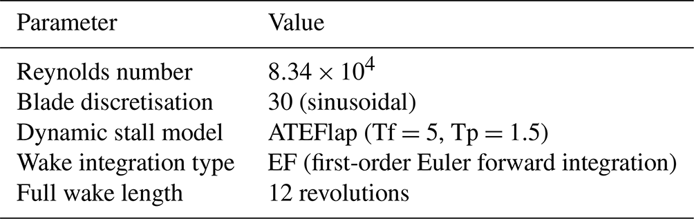
This section details the turbine model (Sect. 2) implementation in QBlade. Note that a rigorous validation procedure has been conducted, encompassing comparison of the actuator cylinder model with the Beddoes–Leishman dynamic stall model (Leishman and Beddoes, 1989) and referenced experimental data (LeBlanc and Simão Ferreira, 2021; LeBlanc and Simão Ferreira, 2022). However, validation results are not explicitly presented in this paper due to scope constraints. To account for the flow curvature effect, a virtual airfoil geometry was computed for the NACA 0021 blade geometry using the transformation technique based on the chord-to-radius ratio available in QBlade (Bianchini et al., 2015). Lift and drag polars for the blades and the struts are computed at a Reynolds number of 8.34×10⁴ with Ncrit=7 and free transition. The polars are then extrapolated with the Montgomerie method (Montgomerie, 2004). In order to enhance the accuracy of the aerodynamic estimation, the ATEFlap model (Bergami and Gauanaa, 2012) has been selected as a dynamic stall model with a boundary layer pressure lag time constant (Tf) of 5 and a peak pressure lag time constant (Tp) of 1.5. The main settings for the QBlade turbine model are summarised in Table C1. The interested reader is referred to Marten et al. (2021) for further explanations of the listed quantities.
Code and data are available at https://doi.org/10.4121/34b8d260-049a-4f7c-b3cd-60f1f4019696 (Brandetti, 2024).
LB: conceptualisation, methodology, software, validation, investigation, visualisation, writing (original draft). SPM: conceptualisation, methodology, supervision, investigation, writing (review and editing). RMM: conceptualisation, methodology, supervision, investigation, writing (review and editing). SW: resources, supervision, writing (review). JWvW: conceptualisation, methodology, supervision, resources, writing (review).
At least one of the (co-)authors is a member of the editorial board of Wind Energy Science. The peer-review process was guided by an independent editor, and the authors also have no other competing interests to declare.
Publisher's note: Copernicus Publications remains neutral with regard to jurisdictional claims made in the text, published maps, institutional affiliations, or any other geographical representation in this paper. While Copernicus Publications makes every effort to include appropriate place names, the final responsibility lies with the authors.
This paper was edited by Alessandro Bianchini and reviewed by David Wood and one anonymous referee.
Afshari, A., Mojahed, M., and Yusuff, R.: Simple Additive Weighting Approach to Personnel Selection Problem, International Journal of Innovation, Management and Technology, 1, 511–515, 2010. a
Aures, W.: Procedure for calculating the sensory euphony of arbitrary sound signal [Berechnungsverfahren für den sensorischen Wohlklang beliebiger Schallsignale], Acustica, 59, 130–141, 1985. a
Bagočius, V., Zavadskas, E. K., and Turskis, Z.: Multi-person selection of the best wind turbine based on the multi-criteria integrated additive-multiplicative utility function, J. Civ. Eng. Manag., 20, 590–599, https://doi.org/10.3846/13923730.2014.932836, 2014. a
Balduzzi, F., Bianchini, A., Carnevale, E. A., Ferrari, L., and Magnani, S.: Feasibility analysis of a Darrieus vertical-axis wind turbine installation in the rooftop of a building, Appl. Energ., 97, 921–929, https://doi.org/10.1016/j.apenergy.2011.12.008, 2012. a, b
Bergami, L. and Gauanaa, M.: ATEFlap Aerodynamic Model: A Dynamic Stall Model Including the Effects of Trailing Edge Flap Deflection, Tech. rep., Technical University of Denmark, https://backend.orbit.dtu.dk/ws/portalfiles/portal/6599679/ris-r-1792.pdf (last access: 10 January 2024), 2012. a
Bianchini, A., Balduzzi, F., Rainbird, J. M., Peiro, J., Graham, J. M. R., Ferrara, G., and Ferrari, L.: An Experimental and Numerical Assessment of Airfoil Polars for Use in Darrieus Wind Turbines–Part I: Flow Curvature Effects, J. Eng. Gas Turb. Power, 138, 032602, https://doi.org/10.1115/1.4031269, 2015. a
Bianchini, A., Bangga, G., Baring-Gould, I., Croce, A., Cruz, J. I., Damiani, R., Erfort, G., Simao Ferreira, C., Infield, D., Nayeri, C. N., Pechlivanoglou, G., Runacres, M., Schepers, G., Summerville, B., Wood, D., and Orrell, A.: Current status and grand challenges for small wind turbine technology, Wind Energ. Sci., 7, 2003–2037, https://doi.org/10.5194/wes-7-2003-2022, 2022. a, b, c
Bonaccorso, F., Scelba, G., Consoli, A., and Muscato, G.: EKF – based MPPT control for vertical axis wind turbines, in: IECON 2011 – 37th Annual Conference of the IEEE Industrial Electronics Society, 7–10 November 2011, Melbourne, VIC, Australia, 3614–3619, https://doi.org/10.1109/IECON.2011.6119896, 2011. a, b
Bossanyi, E. A.: The design of closed-loop controllers for wind turbines, Wind Energy, 3, 149–163, https://doi.org/10.1002/we.34, 2000. a, b, c
Botha, J. D. M., Shahroki, A., and Rice, H.: An implementation of an aeroacoustic prediction model for broadband noise from a vertical axis wind turbine using a CFD informed methodology, J. Sound Vib., 410, 389–415, https://doi.org/10.1016/j.jsv.2017.08.038, 2017. a
Brandetti, L.: Codes, data and plots underlying the publication: Multi-objective calibration of vertical-axis wind turbine controllers: balancing aero-servo-elastic performance and noise, Version 1, 4TU.ResearchData [code and data set], https://doi.org/10.4121/34b8d260-049a-4f7c-b3cd-60f1f4019696, 2024. a
Brandetti, L. and van den Berg, D.: QBlade 2.0.5.2 Matlab Tutorial, Tech. rep., https://doi.org/10.4121/22134710, 2023. a
Brandetti, L., Liu, Y., Mulders, S. P., Ferreira, C., Watson, S., and van Wingerden, J. W.: On the ill-conditioning of the combined wind speed estimator and tip-speed ratio tracking control scheme, J. Phys. Conf. Ser., 2265, 032085, https://doi.org/10.1088/1742-6596/2265/3/032085, 2022. a
Brandetti, L., Avallone, F., De Tavernier, D., LeBlanc, B., Simão Ferreira, C., and Casalino, D.: Assessment through high-fidelity simulations of a low-fidelity noise prediction tool for a vertical-axis wind turbine, J. Sound Vib., 547, 117486, https://doi.org/10.1016/j.jsv.2022.117486, 2023a. a, b, c, d, e
Brandetti, L., Mulders, S. P., Liu, Y., Watson, S., and van Wingerden, J.-W.: Analysis and multi-objective optimisation of wind turbine torque control strategies, Wind Energ. Sci., 8, 1553–1573, https://doi.org/10.5194/wes-8-1553-2023, 2023b. a, b, c, d, e, f, g, h, i, j, k
Brooks, T. F. and Burley, C. L.: Rotor broadband noise prediction with comparison to model data, J. Am. Helicopter Soc., 49, 28–42, 2004. a
Brooks, T. F., Pope, S., and Marcolini, M. A.: Airfoil Self-Noise and Prediction, NASA Reference Publication 1218, 1–142, https://doi.org/10.1080/09524622.2008.9753825, 1989. a, b, c, d, e, f, g
Buck, S., Oerlemans, S., and Palo, S.: Experimental characterization of turbulent inflow noise on a full-scale wind turbine, J. Sound Vib., 385, 219–238, 2016. a, b
Burton, T., Jenkings, N., Sharpe, D., and Bossanyi, E. A.: Wind Energy Handbook, John Wiley & Sons, Ltd, ISBN 9781119992714, https://doi.org/10.1002/9781119992714, 2001. a
Clifton-Smith, M. J.: Aerodynamic Noise Reduction for Small Wind Turbine Rotors, Wind Eng., 34, 403–420, https://doi.org/10.1260/0309-524X.3.4.403, 2010. a
Daniel, P. and Webber, R.: Psychoacoustical Roughness: Implementation of an Optimized Model, Acustica, 83, 113–23, 1997. a
Dayan, E.: Wind energy in buildings: Power generation from wind in the urban environment – where it is needed most, Refocus, 7, 33–38, https://doi.org/10.1016/S1471-0846(06)70545-5, 2006. a
De Tavernier, D. M. A.: Aerodynamic advances in vertical-axis wind turbines, PhD thesis, TU Delft, Delft, https://doi.org/10.4233/uuid:7086f01f-28e7-4e1b-bf97-bb3e38dd22b9, 2021. a, b
Di, G. Q., Chen, X. W., Song, K., Zhou, B., and Pei, C. M.: Improvement of Zwicker's psychoacoustic annoyance model aiming at tonal noises, Appl. Acoust., 105, 164–170, https://doi.org/10.1016/j.apacoust.2015.12.006, 2016. a, b, c
Eriksson, S., Bernhoff, H., and Leijon, M.: Evaluation of different turbine concepts for wind power, Renew. Sust. Energ. Rev., 12, 1419–1434, https://doi.org/10.1016/j.rser.2006.05.017, 2008. a, b
Eriksson, S., Kjellin, J., and Bernhoff, H.: Tip speed ratio control of a 200 kW VAWT with synchronous generator and variable DC voltage, Energy Sci. Eng., 1, 135–143, https://doi.org/10.1002/ese3.23, 2013. a
Fastl, H. and Zwicker, E.: Psychoacoustics – Facts and models, Springer, Berlin, Heidelberg, https://doi.org/10.1007/978-3-540-68888-4, 2007. a, b
Gambier, A.: Multiobjective Optimal Control of Wind Turbines: A Survey on Methods and Recommendations for the Implementation, Energies, 15, 567, https://doi.org/10.3390/en15020567, 2022. a
Greco, G. F., Merino-Martínez, R., and Osses, A.: SQAT: a MATLAB-based toolbox for quantitative sound quality analysis, in: Inter-Noise 2023: 52nd International Congress and Exposition on Noise Control Engineering Location of Conference, 20—23 August 2023, Chiba, Japan, 12 pp., https://doi.org/10.3397/IN_2023_1075, 2023a. a, b
Greco, G. F., Merino-Martínez, R., and Osses, A.: SQAT: a sound quality analysis toolbox for MATLAB, https://doi.org/10.5281/zenodo.7934709, 2023b. a, b
Haque, M. E., Negnevitsky, M., and Muttaqi, K. M.: A Novel Control Strategy for a Variable Speed Wind Turbine with a Permanent Magnet Synchronous Generator, in: 2008 IEEE Industry Applications Society Annual Meeting, 5–9 October 2008, Edmonton, AB, Canada, 1–8, https://doi.org/10.1109/08IAS.2008.374, 2008. a
Holley, W., Rock, S., and Chaney, K.: Control of variable speed wind turbines below-rated wind speed, Proceedings of the 3rd ASME/JSME Conference, ASME/JSME, 18–23 July 1999, San Francisco, California, USA, https://search.worldcat.org/title/42269277 2023 (last access: 15 September 2023), 1999. a
Howell, R., Qin, N., Edwards, J., and Durrani, N.: Wind tunnel and numerical study of a small vertical axis wind turbine, Renew. Energ., 35, 412–422, https://doi.org/10.1016/j.renene.2009.07.025, 2010. a
Hutchinson, M. and Zhao, F.: Global Wind Report 2023, Tech. rep., https://gwec.net/wp-content/uploads/2023/03/GWR-2023_interactive_v2_compressed.pdf (last access: 15 June 2023), 2023. a
International Organization for Standardization: ISO norm 532–1 – Acoustics – Method for calculating loudness – Zwicker method, Tech. rep., https://www.iso.org/obp/ui/en/#iso:std:iso:532:-1:ed-1:v2:en (last access: 28 December 2023), 2017. a
Jonkman, J., Butterfield, S., Musial, W., and Scott, G.: Definition of a 5 MW Reference Wind Turbine for Offshore System Development, Tech. rep., NREL/TP-500-38060, NREL, https://www.nrel.gov/docs/fy09osti/38060.pdf (last access: 18 May 2023), 2009. a
Khan, M., Alavi, M., Mohan, N., Azeez, A., Shanif, A., and Javed, B.: Wind Turbine design and fabrication to power street lights, in: vol. 108, 25–27 February 2017, Malacca, Malaysia, https://doi.org/10.1051/matecconf/201710808010, 2017. a
Kim, J. W., Haeri, S., and Joseph, P. F.: On the reduction of aerofoil-turbulence interaction noise associated with wavy leading edges, J. Fluid Mech., 792, 526–552, https://doi.org/10.1017/jfm.2016.95, 2016. a
Klok, C. W., Kirkels, A. F., and Alkemade, F.: Impacts, procedural processes, and local context: Rethinking the social acceptance of wind energy projects in the Netherlands, Energy Research & Social Science, 99, 103044, https://doi.org/10.1016/j.erss.2023.103044, 2023. a
Lao, Y., Rotea, M. A., Koeln, J. P., Sakib, M. S., and Griffith, D. T.: Economic Nonlinear Model Predictive Control of Offshore Vertical-Axis Wind Turbines, 2022 American Control Conference (ACC), 8–10 June 2022, Atlanta, GA, USA, 3518–3525, https://doi.org/10.23919/ACC53348.2022.9867846, 2022. a
Lara, M., Garrido, J., Ruz, M. L., and Vázquez, F.: Multi-objective optimization for simultaneously designing active control of tower vibrations and power control in wind turbines, Energy Reports, 9, 1637–1650, https://doi.org/10.1016/j.egyr.2022.12.141, 2023a. a, b, c
Lara, M., Garrido, J., van Wingerden, J. W., Mulders, S. P., and Vázquez, F.: Optimization with genetic algorithms of individual pitch control design with and without azimuth offset for wind turbines in the full load region, in: 22nd IFAC World Congress, 9–14 July 2023, Yokohama, Japan, 375–380, https://doi.org/10.1016/j.ifacol.2023.10.1591, 2023b. a
LeBlanc, B. and Simão Ferreira, C.: Estimation of blade loads for a variable pitch vertical axis wind turbine from particle image velocimetry, Wind Energy, 25, 313–332, https://doi.org/10.1002/we.2674, 2021. a, b, c, d
LeBlanc, B. and Simão Ferreira, C.: Estimation of blade loads for a variable pitch Vertical Axis Wind Turbine with strain gage measurements, Wind Energy, 25, 1030–1045, https://doi.org/10.1002/we.2713, 2022. a
Lee, H.-C. and Chang, C.-T.: Comparative analysis of MCDM methods for ranking renewable energy sources in Taiwan, Renew. Sust. Energ. Rev., 92, 883–896, https://doi.org/10.1016/j.rser.2018.05.007, 2018. a
Leishman, J. and Beddoes, T.: A Semi-Empirical Model for Dynamic Stall, J. Am. Helicopter Soc., 34, 3–17, https://doi.org/10.4050/JAHS.34.3.3, 1989. a
Liu, Y., Pamososuryo, A. K., Ferrari, R. M. G., and van Wingerden, J. W.: The Immersion and Invariance Wind Speed Estimator Revisited and New Results, IEEE Control Systems Letters, 6, 361–366, https://doi.org/10.1109/LCSYS.2021.3076040, 2022. a
Lowson, M. V. and Ollerhead, J. B.: A theoretical study of helicopter noise, J. Sound Vib., 9, 197–222, 1969. a
Lukovic, M. K., Tian, Y., and Matusik, W.: Diversity-guided multi-objective Bayesian optimization with batch evaluations, in: 34th Conference on Neural Information Processing Systems, 6–12 December 2020, Vancouver, Canada, https://proceedings.neurips.cc/paper_files/paper/2020/file/cd3109c63bf4323e6b987a5923becb96-Paper.pdf (last access: 31 August 2023), 2020. a, b
Madsen, H. A.: The Actuator Cylinder – A Flow Model for Vertical Axis Wind Turbines, PhD thesis, https://doi.org/10.13140/RG.2.1.2512.3040, 1982. a
Maillard, J., Bresciani, A. P. C., and Finez, A.: Perceptual validation of wind turbine noise auralization, in: Proceedings of the 10th Convention of the European Acoustics Association (Forum Acusticum), 11–15 September 2023, Turin, Italy, https://doi.org/10.61782/fa.2023.0444, 2023. a, b
Marten, D.: QBlade: a modern tool for the aeroelastic simulation of wind turbines, PhD thesis, https://doi.org/10.14279/depositonce-10646, 2020. a, b, c, d, e
Marten, D., Saverin, J., Behrens de Luna, R., and Perez-Becker, S.: QBlade documentation, Tech. rep., https://docs.qblade.org/ (last access: 27 December 2023), 2021. a
Merino-Martínez, R., Pieren, R., and Schäffer, B.: Holistic approach to wind turbine noise: From blade trailing-edge modifications to annoyance estimation, Renew. Sust. Energ. Rev., 148, 111285, https://doi.org/10.1016/j.rser.2021.111285, 2021. a, b, c, d, e, f, g
Merino-Martínez, R., Pieren, R., Schäffer, B., and Simons, D.: Psychoacoustic model for predicting wind turbine noise annoyance, https://www.researchgate.net/publication/364996997_Psychoacoustic_model_for_predicting_wind_turbine_noise_annoyance (last access: 10 September 2023), 2022. a, b
Mertens, S., van Kuik, G., and van Bussel, G.: Performance of an H-Darrieus in the Skewed Flow on a Roof, J. Sol. Energ.-T. ASME, 125, 433–440, https://doi.org/10.1115/1.1629309, 2003. a
Miettinen, K.: Nonlinear multiobjective optimization, Springer, https://doi.org/10.1007/978-1-4615-5563-6, 1999. a
Montgomerie, B.: Methods for Root Effects, Tip Effects and Extending the Angle of Attack Range to 6180, With Application to Aerodynamics for Blades on Wind Turbines and Propellers, Tech. rep., Swedish Defence Research Agency, https://www.foi.se/rest-api/report/FOI-R--1305--SE (last access: 20 August 2023), 2004. a
Moriarty, P. and Migliore, P.: Semi-Empirical Aeroacoustic Noise Prediction Code for Wind Turbines, Tech. rep., NREL – National Renewable Energy Laboratory, https://www.nrel.gov/docs/fy04osti/34478.pdf (last access: 30 December 2023), 2003. a
Moustakis, N., Mulders, S. P., Kober, J., and van Wingerden, J. W.: A Practical Bayesian Optimization Approach for the Optimal Estimation of the Rotor Effective Wind Speed, in: 2019 American Control Conference (ACC), 10–12 July 2019, Philadelphia, PA, USA, 4179–4185, https://doi.org/10.23919/ACC.2019.8814622, 2019. a
Odgaard, P. F., Larsen, L. F. S., Wisniewski, R., and Hovgaard, T. G.: On using Pareto optimality to tune a linear model predictive controller for wind turbines, Renew. Energ., 87, 884–891, https://doi.org/10.1016/j.renene.2015.09.067, 2016. a
Ortega, R., Mancilla-David, F., and Jaramillo, F.: A globally convergent wind speed estimator for wind turbine systems, Int. J. Adapt. Control, 27, 413–425, https://doi.org/10.1002/acs.2319, 2013. a
Osses Vecchi, A., García León, R., and Kohlrausch, A.: Modelling the sensation of fluctuation strength, in: vol. 28 of Proceedings of Meetings on Acoustics, 5–9 September 2016, Buenos Aires, Brazil, https://doi.org/10.1121/2.0000410, 2016. a
Østergaard, K. Z., Brath, P., and Stoustrup, J.: Estimation of effective wind speed, J. Phys. Conf. Ser., 75, 012082, https://doi.org/10.1088/1742-6596/75/1/012082, 2007. a
Papi, F., Nocentini, A., Ferrara, G., and Bianchini, A.: On the Use of Modern Engineering Codes for Designing a Small Wind Turbine: An Annotated Case Study, Energies, 14, 1013, https://doi.org/10.3390/en14041013, 2021. a
Pieren, R., Heutschi, K., Müller, M., Manyoky, M., and Eggenschwiler, K.: Auralization of Wind Turbine Noise: Emission Synthesis, Acta Acust. United Ac., 100, 25–33, https://doi.org/10.3813/AAA.918683, 2014. a
Pieren, R., Bertsch, L., Lauper, D., and Schäffer, B.: Improving Future Low-noise Aircraft Technologies Using Experimental Perception-Based Evaluation of Synthetic Flyovers, Sci. Total Environ., 692, 68–81, https://doi.org/10.1016/j.scitotenv.2019.07.253, 2019. a, b
Poulsen, A. H., Raaschou-Nielsen, O., Peña, A., Hahmann, A. N., Nordsborg, R. B., Ketzel, M., Brandt, J., and Sørensen, M.: Impact of Long-Term Exposure to Wind Turbine Noise on Redemption of Sleep Medication and Antidepressants: A Nationwide Cohort Study, Environ. Health Persp., 127, 037005, https://doi.org/10.1289/EHP3909, 2019. a
Pourrajabian, A., Rahgozar, S., Dehghan, M., and Wood, D.: A comprehensive multi-objective optimization study for the aerodynamic noise mitigation of a small wind turbine, Eng. Anal. Bound. Elem., 155, 553–564, https://doi.org/10.1016/j.enganabound.2023.06.035, 2023. a
Ramirez, L.: Offshore wind energy: 2023 statistics, Tech. rep., https://windeurope.org/intelligence-platform/product/offshore-wind-in-europe-key-trends-and-statistics-2022/ (last access: 15 August 2023), 2023. a
Rogers, A. L., Manwell, J. F., and Wright, S.: Wind turbine acoustic noise, Tech. rep., https://doi.org/10.1260/0957456042872777, 2006. a, b
Ruijgrok, G. J. J.: Elements of Aviation Acoustics, Cambridge University Press, https://doi.org/10.1017/S0001924000027056, 1993. a
Santín, I., Pedret, C., and Vilanova, R.: Control and Decision Strategies in Wastewater Treatment Plants for Operation Improvement, Intelligent Systems, Springer, https://doi.org/10.1007/978-3-319-46367-4, 2017. a
Sessarego, M. and Wood, D.: Multi-dimensional optimization of small wind turbine blades, Renewables: Wind, Water, and Solar, 9, 9, https://doi.org/10.1186/s40807-015-0009-x, 2015. a
Simão Ferreira, C. J., van Kuik, G., van Bussel, G., and Scarano, F.: Visualization by PIV of dynamic stall on a vertical axis wind turbine, Exp. Fluids, 97–108, https://doi.org/10.1007/s00348-008-0543-z, 2009. a
Soltani, M. N., Knudsen, T., Svenstrup, M., Wisniewski, R., Brath, P., Ortega, R., and Johnson, K.: Estimation of rotor effective wind speed: A comparison, IEEE T. Contr. Syst. T., 21, 1155–1167, https://doi.org/10.1109/TCST.2013.2260751, 2013. a
Veers, P., Dykes, K., Lantz, E., Barth, S., Bottasso, C. L., Carlson, O., Clifton, A., Green, J., Green, P., Holttinen, H., Laird, D., Lehtomäki, V., Lundquist, J. K., Manwell, J., Marquis, M., Meneveau, C., Moriarty, P., Munduate, X., Muskulus, M., Naughton, J., Pao, L., Paquette, J., Peinke, J., Robertson, A., Rodrigo, J. S., Sempreviva, A. M., Smith, J. C., Tuohy, A., and Wiser, R.: Grand challenges in the science of wind energy, Science, 366, 6464, https://doi.org/10.1126/science.aau2027, 2019. a, b
von Bismarck, G.: Sharpness as an attribute of the timbre of steady sounds, Acustica, 30, 159–172, 1974. a
Vorländer, M.: Auralization – Fundamentals of Acoustics, Modelling, Simulation, Algorithms and Acoustic Virtual Reality, Springer, ISBN 978-3-540-48830-9, https://doi.org/10.1007/978-3-540-48830-9, 2008. a, b, c
Wang, P., Zhu, Z., and Wang, Y.: A novel hybrid MCDM model combining the SAW, TOPSIS and GRA methods based on experimental design, Inform. Sciences, 345, 27–45, https://doi.org/10.1016/j.ins.2016.01.076, 2016. a, b, c
Watson, S., Moro, A., Reis, V., Baniotopoulos, C., Barth, S., Bartoli, G., Bauer, F., Boelman, E., Bosse, D., Cherubini, A., Croce, A., Fagiano, L., Fontana, M., Gambier, A., Gkoumas, K., Golightly, C., Latour, M. I., Jamieson, P., Kaldellis, J., Macdonald, A., Murphy, J., Muskulus, M., Petrini, F., Pigolotti, L., Rasmussen, F., Schild, P., Schmehl, R., Stavridou, N., Tande, J., Taylor, N., Telsnig, T., and Wiser, R.: Future emerging technologies in the wind power sector: A European perspective, Renew. Sust. Energ. Rev., 113, 109270, https://doi.org/10.1016/j.rser.2019.109270, 2019. a, b, c
- Abstract
- Introduction
- Notations
- Vertical-axis wind turbine
- Theory and derivations of wind turbine controllers
- Methodology to assess the noise levels and psychoacoustic annoyance on a VAWT
- Multi-objective optimisation and implementation of the WSE–TSR tracking controller
- Results
- Conclusions
- Appendix A: Airfoil self-noise model
- Appendix B: Turbulence–interaction noise model
- Appendix C: QBlade turbine model
- Code and data availability
- Author contributions
- Competing interests
- Disclaimer
- Review statement
- References