the Creative Commons Attribution 4.0 License.
the Creative Commons Attribution 4.0 License.
 | 14 Mar 2024
Seasonal variability of wake impacts on US mid-Atlantic offshore wind plant power production
David Rosencrans
Julie K. Lundquist
Mike Optis
Alex Rybchuk
Nicola Bodini
Michael Rossol
The mid-Atlantic will experience rapid wind plant development due to its promising wind resource located near large population centers. Wind turbines and wind plants create wakes, or regions of reduced wind speed, that may negatively affect downwind turbines and plants. We evaluate wake variability and annual energy production with the first yearlong modeling assessment using the Weather Research and Forecasting model, deploying 12 MW turbines across the domain at a density of 3.14 MW km−2, matching the planned density of 3 MW km−2. Using a series of simulations with no wind plants, one wind plant, and complete build-out of lease areas, we calculate wake effects and distinguish the effect of wakes generated internally within one plant from those generated externally between plants. We also provide a first step towards uncertainty quantification by testing the amount of added turbulence kinetic energy (TKE) by 0 % and 100 %. We provide a sensitivity analysis by additionally comparing 25 % and 50 % for a short case study period. The strongest wakes, propagating 55 km, occur in summertime stable stratification, just when New England's grid demand peaks in summer. The seasonal variability of wakes in this offshore region is much stronger than the diurnal variability of wakes. Overall, yearlong simulated wake impacts reduce power output by a range between 38.2 % and 34.1 % (for 0 %–100 % added TKE). Internal wakes cause greater yearlong power losses, from 29.2 % to 25.7 %, compared to external wakes, from 14.7 % to 13.4 %. The overall impact is different from the linear sum of internal wakes and external wakes due to non-linear processes. Additional simulations quantify wake uncertainty by modifying the added amount of turbulent kinetic energy from wind turbines, introducing power output variability of 3.8 %. Finally, we compare annual energy production to New England grid demand and find that the lease areas can supply 58.8 % to 61.2 % of annual load. We note that the results of this assessment are not intended to make nor are they suitable to make commercial judgments about specific wind projects.
- Article
(10384 KB) - Full-text XML
- BibTeX
- EndNote


The US offshore wind industry is flourishing, with a target capacity of 30 GW by 2030 (FACT SHEET, 2023). New England features the highest population density in the United States and commensurate utility usage, making offshore wind an attractive regional electricity source. A total of 27 active lease areas now span the mid-Atlantic Outer Continental Shelf (OCS). The OCS features low turbulence (Bodini et al., 2019) and fast winds, with 100 m winds averaging 10 m s−1 (Musial et al., 2016). Consequently, large wind plants will be constructed to harness the ample wind resource.
Meteorological conditions and construction challenges constrain siting options for large wind plants. Because the average wind direction is southwesterly (Bodini et al., 2019), a southwest-to-northeast wind plant orientation mitigates external waking from neighboring plants. Further, preserving efficient vessel transit, upholding common fishery practices, and prioritizing safe Coast Guard search-and-rescue operations necessitate 1×1 nm corridors (W.F. Baird & Associates, 2019). Considering these constraints, wind plants will be densely packed into clusters.
Densely packed clusters produce wakes that adversely affect downwind turbines (Nygaard, 2014; Platis et al., 2018; Lundquist et al., 2019; Schneemann et al., 2020). Wakes are plumes downwind of turbines with slower wind speeds and increased turbulence. Mid-Atlantic wakes induced by large wind plants could impose wind speed deficits up to 2 m s−1 (Pryor et al., 2021; Golbazi et al., 2022). Wind speed deficits can be replenished by wake recovery in which turbulence entrains momentum from aloft into the waked zone (Stevens et al., 2016; Gupta and Baidya Roy, 2021). However, stably stratified conditions suppress mixing for wake recovery (Fitch et al., 2013; Vanderwende et al., 2016; Porté-Agel et al., 2020). Under certain conditions, mid-Atlantic wakes could propagate 100 km or more (Pryor et al., 2021; Golbazi et al., 2022; Stoelinga et al., 2022).
Wake characteristics have been evaluated using physics-based models of varying complexity. High-fidelity methods include computational fluid dynamics models solving Reynolds-averaged Navier–Stokes equations (Antonini et al., 2020); large-eddy simulations resolving the turbine rotor as an actuator disk (Mirocha et al., 2014; Aitken et al., 2014; Shapiro et al., 2019; Arthur et al., 2020); and mesoscale models parameterizing a hub-height momentum sink, sometimes including a turbulence source (Fitch et al., 2013; Volker et al., 2015; Archer et al., 2020; Gupta and Baidya Roy, 2021), as reviewed by Fischereit et al. (2022). Pryor et al. (2021) characterized mid-Atlantic wake impacts using mesoscale modeling of 55 simulation days. They examined modified wind plant layouts of 15 MW turbines under different flow scenarios, considering power densities between 2.1 and 4.34 MW km−2. Stoelinga et al. (2022) estimated wake impacts using 15 MW turbines and 16 simulation days under typical southwesterly flow. Golbazi et al. (2022) considered summertime wakes with three scales of turbines to consider surface impacts. Finally, Rybchuk et al. (2022) addressed the sensitivity to wake characteristics under idealized conditions by varying planetary boundary layer (PBL) schemes.
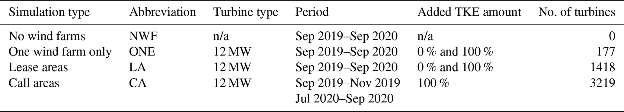
In this work, we assess intra-plant and inter-plant wakes throughout the mid-Atlantic OCS using a yearlong mesoscale modeling study. The results of this assessment are not intended to make nor are they suitable to make commercial judgments about specific wind projects. The simulations use the Weather Research and Forecasting (WRF) model version 4.2.1 (Skamarock et al., 2019). One set of simulations runs with no wind farms (NWF) as a control, validated with lidar measurements, while the others use the Fitch wind farm parameterization (WFP) (Fitch et al., 2012, with updates described by Archer et al., 2020) to incorporate turbine effects. Our simulations incorporate 12 MW turbines and a power density of 3.14 MW km−2. Simulations employ different wind plant layouts, including one representative lease area alone (ONE) within the Rhode Island–Massachusetts (RIMA) block, all lease areas (LA), and the lease areas plus the call areas (CA), to assess different waking scenarios (Table 1). WFP simulations run separately by added turbulent kinetic energy (TKE) amount, including 0 % added TKE (TKE_0) and 100 % added TKE (TKE_100) to quantify the full range of uncertainty. NWF, ONE, and LA simulations run from 1 September 2019 to 1 September 2020 to capture a full year with available lidar measurement data. Due to computational costs, CA simulations focus on the summertime stable period from 1 September to 31 October 2019 and 1 July to 31 August 2020 (Table 1). This time period highlights wake impacts during months with presumed frequent stable stratification and high electricity demands (Livingston and Lundquist, 2020) as a worst-case scenario.
The remainder of this article is structured as follows. Section 2 introduces the model setup and configuration, model validation, and the analysis methods. Section 3 discusses variability in stratification, wakes, and power production. Section 4 concludes the work and offers recommendations for future work.
2.1 WRF modeling setup
We assess the effects of wakes and power production across the mid-Atlantic OCS using numerical weather prediction simulations with WRF version 4.2.1 and the WFP (Fitch et al., 2012). Version 4.2.1 allows for modifying the amount of TKE produced by wind turbines and ensures turbulence advection (Archer et al., 2020). Two nested domains comprise 6 and 2 km horizontal resolutions (Pronk et al., 2022; Xia et al., 2022; Bodini et al., 2023; Redfern et al., 2023), respectively, and the inner nest begins 20 grid cells into the parent domain (Fig. 1). This same domain and period of study have been used to explore interactions between power production and sea breezes (Xia et al., 2022). Fine vertical resolution (10 m) near the surface stretches aloft, with 17 levels within the lowest 200 m as recommended by Tomaszewski and Lundquist (2020). We choose an 18 s time step in the outer domain, 54 vertical levels, a 5000 Pa top, simple diffusion, and damping 6000 m below the model top to prevent gravity wave reflection. Hourly 30 km initial and boundary conditions are provided by the European Centre for Medium-Range Weather Forecasts (ECMWF) fifth-generation reanalysis (ERA5) data set (Hersbach et al., 2020). Sea surface temperature is provided by the UK Met Office Operational Sea Surface Temperature and Sea Ice Analysis (OSTIA) data set (Donlon et al., 2012). We choose the Noah land surface model (Niu et al., 2011), the Mellor–Yamada–Nakanishi and Niino level 2.5 PBL and surface layer (Nakanishi and Niino, 2006), new Thompson microphysics (Thompson et al., 2008), and the rapid radiative transfer model longwave and shortwave radiative transfer (Iacono et al., 2008) schemes. The Kain–Fritsch cumulus scheme parameterizes cloud microphysics in the outer domain only (Kain, 2004).
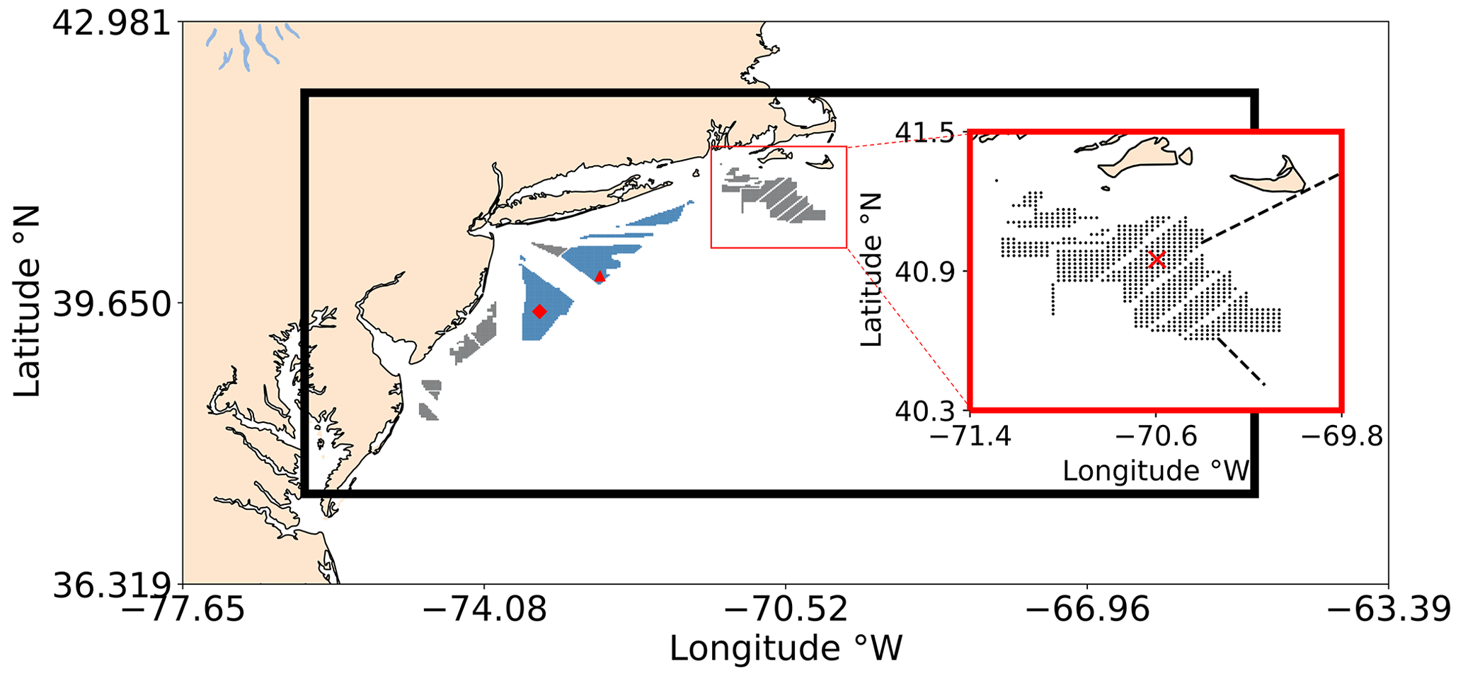
Figure 1Simulation Domain 1 includes the entire region, and Simulation Domain 2 is outlined by the black rectangle. Each dot represents a wind turbine. Wind energy lease areas are shown in gray and call areas in blue. The red square zooms in on the Rhode Island–Massachusetts block of lease areas. The E05 (triangle) and E06 (diamond) floating lidars are shown in red. Atmospheric stratification is assessed at the red X. Wake propagation distances are assessed along the dashed black lines.
2.2 Wind turbine layouts
Wind turbines are sited within lease areas offshore of the US East Coast (Fig. 1) as defined by the Bureau of Ocean Energy Management (Bureau of Ocean Energy Management, 2023). Following realistic deployment strategies, we site individual turbines 1 nm, or 8.6 rotor diameters, apart and an additional 0.5 nm from lease area boundaries (W.F. Baird & Associates, 2019; Beiter et al., 2020; Walter Musial, personal communication, September 2020). This layout provides a power density of 3.14 MW km−2. Lower power densities in US waters reflect wake concerns in Europe and the need to increase turbine spacing for wake replenishment. Areas that had already been approved for development are denoted as the lease areas. Areas where competitive interest was yet to be determined are denoted as the call areas. Both lease areas and call areas are filled to spatial capacity with turbines (Fig. 1), recognizing renewable energy targets (218th Legislature, 2018).
2.3 Wind turbine characteristics
For our simulations, we parameterize 12 MW turbines which are scaled by Beiter et al. (2020) from a 15 MW reference turbine with a 138 m hub height and 215 m rotor diameter. The power and thrust coefficient curves were held constant from the 15 MW machine. The rotor diameter was scaled to maintain a specific power of 332 W m−2, which is the same as the reference 15 MW turbine. Then, the hub height was determined such that a 30 m gap was maintained between the lower bound of the rotor tip and the sea surface. No power is produced in region 1 of the power curve, from 0 m s−1 to cut-in wind speed (3 m s−1). In region 2 of the power curve, power production increases between cut-in wind speed and rated speed (11 m s−1). In region 3, between rated and cut-out wind speed (30 m s−1), an increase in wind speed no longer yields additional power production (Beiter et al., 2020) (Fig. 2a).
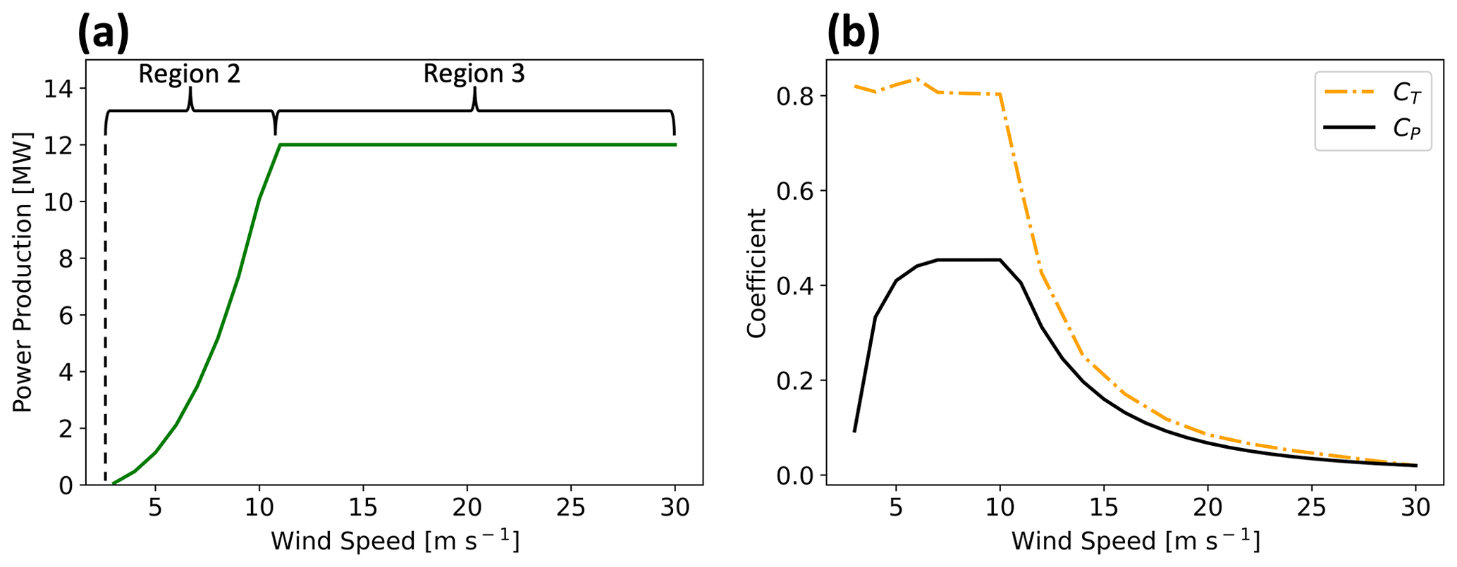
Figure 2Characteristics of the 12 MW scaled turbine used herein. (a) The power curve and (b) curves showing the thrust coefficients (CT; dashed orange) and the power coefficients (CP; solid black) with wind speed across the x axis.
2.4 Wind farm parameterization
We use the WFP (Fitch et al., 2012) to incorporate the effects of wind turbines on the 2 km grid. Horizontal wind speed reduction from turbine drag (Eq. 1), power production (Eq. 2), and turbulence generation (Fitch et al., 2012; Archer et al., 2020) (Eq. 3) are calculated in the WFP from the following:
where i, j, and k represent Cartesian model coordinates; CT(|V|ijk) is the wind-speed-dependent thrust coefficient; |V| is the wind speed at turbine hub height; ρ is the air density; Aijk is the rotor-swept area; Nij is the number density of turbines in grid cell ij; CP(|V|ijk) is the wind-speed-dependent power coefficient; zk is the height of vertical model level k; and CTKE is the fraction of energy converted to TKE (Fitch et al., 2012). These values are calculated at each model level, as the use of a rotor-equivalent wind speed generally exerts a minor effect (Redfern et al., 2019).
The thrust and power coefficients (CT and CP, respectively) vary with wind speed as defined by wind turbine manufacturers (Fig. 2b). The thrust coefficient CT is the non-dimensionalized thrust force exerted by wind on the rotor-swept plane (Burton et al., 2011).
The power coefficient, CP, governs the fraction of rotor kinetic energy converted into electrical power. This conversion is not perfectly efficient due to electrical and mechanical losses (Fitch et al., 2012; Archer et al., 2020). The leftover fraction of energy (Eq. 4) from the difference between CT and Cp is transformed into turbulence, CTKE.
Because electromechanical losses are not represented by the WFP, all leftover energy converts to TKE, so the TKE may be overestimated (Fitch et al., 2012; Archer et al., 2020). Some researchers suggest this TKE term is unnecessary (Volker et al., 2015), although comparisons to large-eddy simulations (Vanderwende et al., 2016) and observations (Siedersleben et al., 2020) suggest the turbine-produced TKE is critical to include. Any overestimation of TKE would enhance turbulent mixing, thereby exaggerating turbulent transport of momentum that causes wake recovery and overestimating power production. Therefore, Archer et al. (2020) propose reducing CTKE to 25 %. For these simulations, we bound this uncertainty by carrying out simulations with 100 % and 0 % added TKE (Fig. A1). TKE advection is turned on.
2.5 Observations
We compared the NWF simulation to observations of offshore wind profiles. Two buoy-mounted meteorological ocean observing systems, denoted E05 and E06, are located within the Hudson North and Hudson South call areas of the New York Bight (Fig. 3). Each buoy system samples line-of-sight boundary layer wind speed and wind direction using the ZephIR ZX300M light detection and ranging (lidar) instrument. The lidars are mounted 2 m above the sea surface and take measurements at 20 m intervals up to 200 m, providing 10 min averages of wind speed and direction, which the New York State Energy Research and Development Authority (NYSERDA) has made publicly available (DNV, 2019). We use floating lidar data to validate simulations for 1 September 2019 to 1 September 2020.
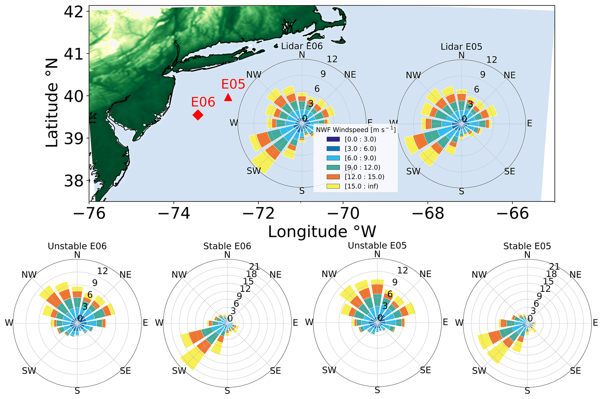
Figure 3Hub-height wind roses for the NYSERDA Hudson North (E05) and Hudson South (E06) floating lidars during the 1 September 2019 to 1 September 2020 period. The location of E06 is shown as the red diamond and E05 as the red triangle. The bottom row shows wind roses segregated by atmospheric stratification.
2.6 Stability classification
Different methods can be used to identify stratification, or atmospheric stability. Stable stratification can occur in coastal regions when warm air advects over a cooler sea surface, thereby suppressing buoyancy and turbulent mixing. Likewise, unstable stratification can occur when cool air advects over a warmer sea surface. Some observations suggest more frequent unstable stratification, based on the Obukhov length (Archer et al., 2016). The sign of the Obukhov length depends on the sign of heat flux and can be a useful metric for determining stability conditions. Other observations suggest that minimal turbulence and strong veer can be characteristic of stable conditions (Bodini et al., 2019). Wind veer increases in stable stratification as the influence of buoyant-turbulence-induced friction decreases. Thus, winds turn to approach quasi-geostrophic flow at a quicker rate, which can be further exaggerated by the presence of a low-level jet.
We calculate the Obukhov length (Monin and Obukhov, 1954) (L), representative of the height at which buoyant production of turbulence first dominates mechanical shear production of turbulence:
where u∗ is the friction velocity (UST from WRF output), θv is the virtual potential temperature, κ is the von Karman constant of 0.4, g is gravitational acceleration, and is the vertical turbulent heat flux (HFX from WRF output). Lengths between 0 and −500 m are characterized as unstable stratification, and lengths between 0 and 500 m are categorized as stable stratification (Muñoz-Esparza et al., 2012). Lengths approaching negative or positive infinity are neutral. Each timestamp from the NWF run is assigned a stability for the 1 September 2019 to 1 September 2020 period at a grid point centered on the RIMA block (Fig. 1).
2.7 Model validation
We validate the NWF model by comparing wind speed estimated by the turbine-free simulations with observations from E05 and E06 lidars. Model output is obtained from the grid cells containing the lidars in 20 m intervals from 60 to 200 m following Pronk et al. (2022). Wind speeds and directions are compared using a suite of metrics recommended by Optis et al. (2020) for wind resource assessment, including the correlation coefficient (r), centered root-mean-square error (cRMSE), and bias:
where V is the wind speed, N is the total number of values, σ is the standard deviation, and subscripts “W” and “L” indicate WRF and lidar, respectively. Earth mover's distance (EMD), or the Wasserstein metric, is calculated with a SciPy function (Virtanen et al., 2020) as in other wind resource evaluations (Hahmann et al., 2020). Each of these metrics provides different insights into the performance of the model. For instance, the correlation coefficient illuminates how well the model captures the timing of weather systems and diurnal variability. EMD emphasizes the difference between distributions but not the timing. Bias captures the difference between measured and modeled values. Finally, cRMSE describes the random component of error.
The circularity of wind direction must be accounted for in statistical calculations. For example, computing the average between 359 and 1°, using a typical arithmetic mean, would result in 180°. However, the mean wind direction between those two values should be 360°. The SciPy (Virtanen et al., 2020) and Astropy (Price-Whelan et al., 2022) Python packages offer convenient functions which allow the user to calculate statistics for a circular variable by passing in the lower and upper bounds, in this case 0 and 360°. We calculate the mean and standard deviation of wind direction using the SciPy circmean and circstd functions, respectively, and the correlation coefficient using the Astropy circcorrcoef function. The cRMSE for wind direction is then calculated following
where D is wind direction, and is the circular mean of wind direction. Bias is calculated similarly to Eq. (8), except that differences between NWF and lidar values that are less than −180° have 360° added and differences greater than 180° have 360° subtracted:
where x is the () difference.
Table 2Percentage of data removed at 140 m due to not-a-number (NaN) values.
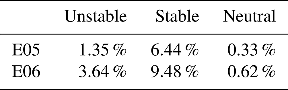
Time stamps in which the lidar returns NaN values are removed from WRF data sets during comparison (Table 2). Doing so removes 8.1 % of wind speed data at 140 m at E05, made up by 1.22 %, 5.76 %, and 1.13 % in unstable, stable, and neutral stratification, respectively. Similarly, 13.7 % of wind speed data are removed at E06 and are made up by 3.20 %, 9.38 %, and 1.15 % in unstable, stable, and neutral stratification, respectively. An r2 value of 1 indicates a perfect correlation between NWF and lidar values. A value of 0 for cRMSE indicates that all values, with model bias removed, lie on the 1:1 regression line. A cRMSE value greater than 0 indicates the distance of residual points from the regression line. Negative biases indicate an underestimation from WRF, while positive biases indicate overestimation. A value of 0 for EMD indicates that probability density functions from each data source are equivalent. A positive EMD indicates that the NWF wind speed distribution must shift towards lower values to match the lidar distribution.
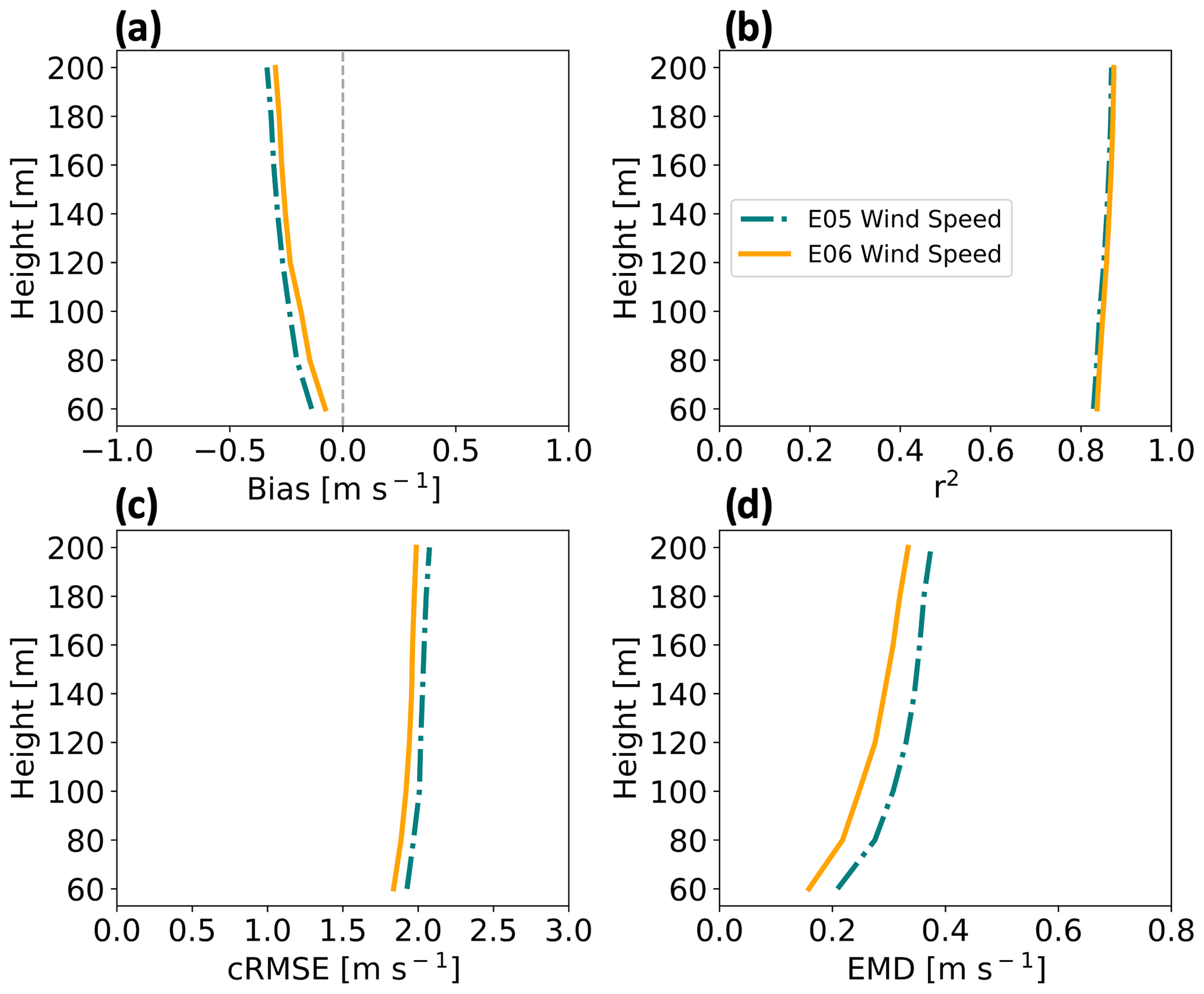
Figure 4Vertical profiles for wind speed comparative metrics at the E05 (teal) and E06 (orange) lidars from 1 September 2019 to 1 September 2020. Shown are (a) bias, (b) correlation, (c) cRMSE, and (d) EMD.
NWF wind speed profiles are compared with lidar observations for the 1 September 2019 to 1 September 2020 period to assess model skill (Fig. 4). Note that Pronk et al. (2022) provide validation metrics against the E05 lidar profile during the same period of study and find similar results. Negative biases (Eq. 8) increase in magnitude with height between 0 and −0.5 m s−1 (Fig. 4a), showing the model underestimates the wind speed. Strengths of variation (Eq. 6) among WRF output and the lidars range between 0.82 and 0.86 (Fig. 4b). Centered RMSE (Eq. 7) increases with height around 2 m s−1 (Fig. 4c). Finally, EMD values originate around 0.2 m s−1 at 60 m and increase with height (Fig. 4d). Comparing lidars E05 and E06, WRF performs better at E06 with a smaller bias by 0.04 m s−1, lower cRMSE by 0.08 m s−1, better correlation by 0.003, and smaller EMD by 0.05 m s−1.
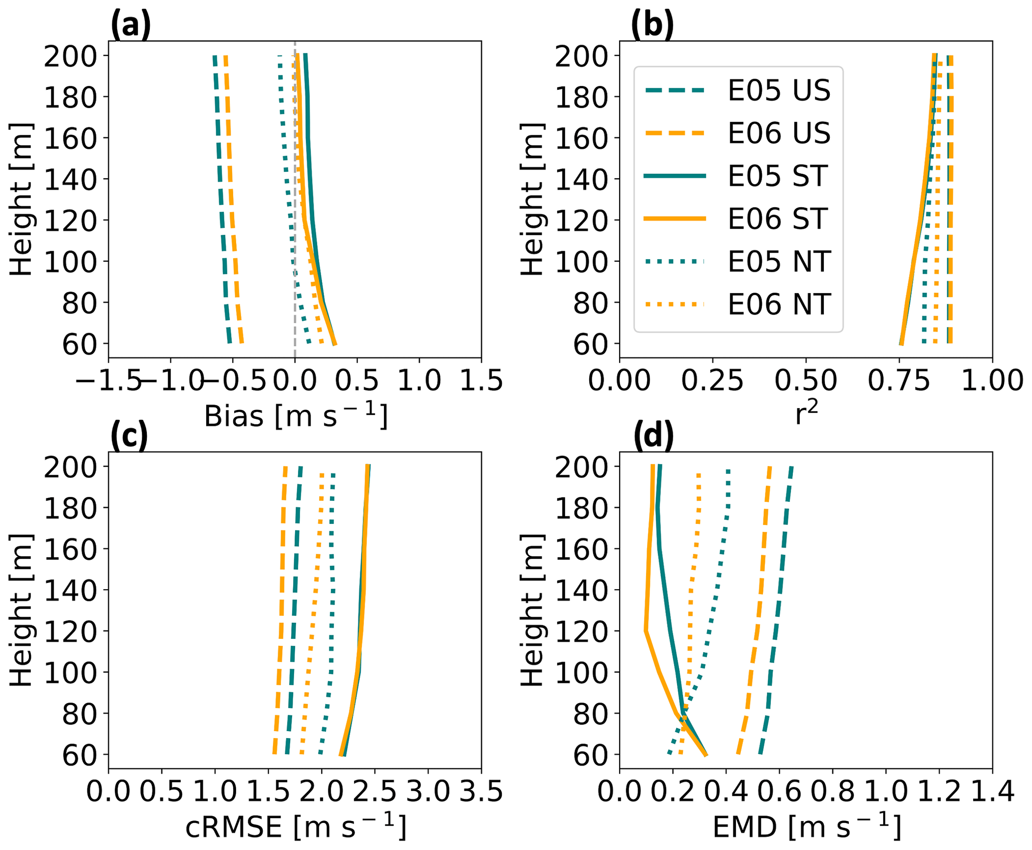
Figure 5Vertical profiles for wind speed comparative metrics at the E05 (teal) and E06 (orange) lidar locations subset by stratification (US – unstable, ST – stable, NT – neutral) from 1 September 2019 to 1 September 2020. Shown are (a) bias, (b) correlation, (c) cRMSE, and (d) EMD.
We further assess the NWF performance, partitioned by stability conditions. In unstable stratification, WRF wind speeds have a negative bias that gradually increases in magnitude with height from −0.5 m s−1 at 60 m (Fig. 5a). In stable conditions, WRF overestimates wind speeds by roughly 0.4 m s−1 at 60 m with biases approaching 0.0 m s−1 further aloft (Fig. 5a). In neutral conditions, WRF overestimates wind speeds by up to 0.3 m s−1 near the surface and underestimates wind speeds further aloft. Comparing between mean E05 and E06 profiles, WRF performs better at the E06 lidar location by 0.08 m s−1 in unstable conditions, 0.04 m s−1 in stable conditions, and 0.1 m s−1 in neutral conditions.
NWF and lidar wind speeds correlate well. Correlation remains the largest in unstable conditions for all heights (Fig. 5b). The worst strength of relationship occurs in stable stratification, although there is improvement aloft, and by 160 m, correlation between stable and neutral conditions is largely equivalent (Fig. 5b). On average, WRF performance between lidar locations is the same in unstable and stable conditions and better at E06 by 0.02 in neutral conditions.
Centered RMSE profiles change with stratification. In unstable conditions, cRMSE increases somewhat with height originating from greater than 1.5 m s−1 at 60 m (Fig. 5c). In stable stratification, the cRMSE profile begins at roughly 2.3 m s−1 at 60 m and increases with height. In neutral conditions, cRMSE increases with height from around 2 m s−1. As before, WRF performs better at E06. On average, cRMSE is lower at E06 by 0.1 m s−1 in unstable conditions, by a negligible amount in stable conditions, and by 0.1 m s−1 in neutral conditions.
Earth mover's distance has more variability with height. It is the largest in unstable stratification, increasing with height from roughly 0.5 m s−1 at 60 m (Fig. 5d). In stable conditions, EMD decreases with height and originates at around 0.35 m s−1 at 60 m. In neutral stratification, EMD decreases with height from about 0.2 m s−1. On average, WRF performs better at E06 by 0.07 m s−1 in unstable conditions, by 0.04 m s−1 in stable conditions, and by 0.06 m s−1 in neutral conditions.
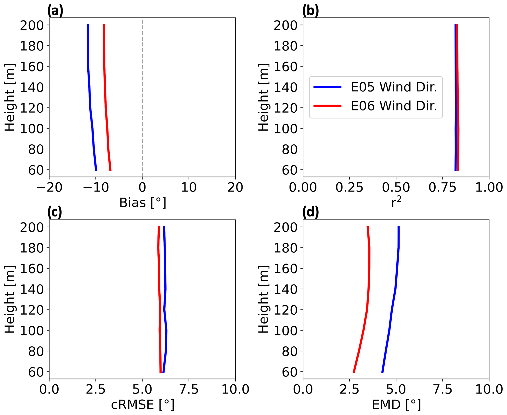
Figure 6Vertical profiles for wind direction comparative metrics at the E05 (blue) and E06 (red) lidar locations from 1 September 2019 to 1 September 2020. Shown are (a) bias, (b) correlation, (c) cRMSE, and (d) EMD.
Next, we show metrics to compare WRF output wind direction profiles with lidar measurements. Bias is negative, or counterclockwise, at both E05 and E06 lidar locations. NWF output resolves wind directions better at E06 with a mean bias of −7.8° with height as compared to −11.1° at E05 (Fig. 6a). Correlation coefficients at both locations are strong, at 0.83 and 0.82 for E06 and E05, respectively (Fig. 6b). Mean cRMSE (Eq. 9) is similar between lidar locations, at 5.9 and 6.2° for E06 and E05, respectively (Fig. 6c). Finally, EMD is lower at E06, increasing with height with an average of 3.3° (Fig. 6d). EMD is larger at E05, increasing with height with an average of 4.8° (Fig. 6d). Overall, WRF performs better at E06 with lower absolute bias by 3.3°, lower RMSE by 0.3°, higher correlation by 0.01, and lower EMD by 1.48°.
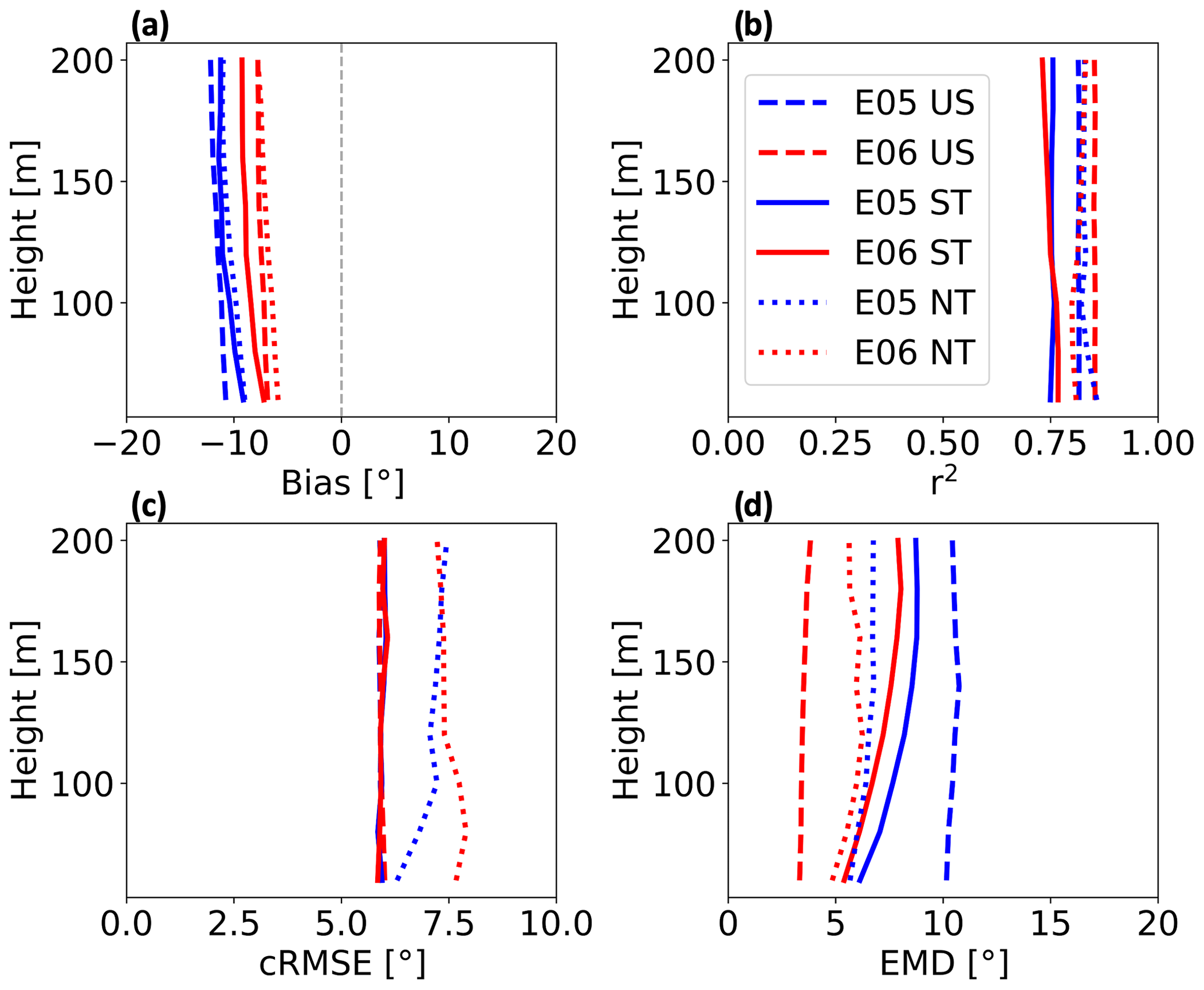
Figure 7Vertical profiles for wind direction comparative metrics at the E05 (blue) and E06 (red) lidar locations subset by stratification (US – unstable, ST – stable, NT – neutral) from 1 September 2019 to 1 September 2020. Shown are (a) bias, (b) correlation, (c) cRMSE, and (d) EMD.
We use the same metrics to validate WRF against lidar-reported wind directions by stratification and begin with bias (Fig. 7a). In unstable conditions, mean biases are −7.4° at E06 and −11.5° at E05. In stable stratification, bias profiles are more similar between lidar locations, reaching −8.6° at E06 and −10.7° at E05. Bias is the smallest in neutral conditions at both locations, with mean values of −6.8° at E06 and −10.2° at E05. Overall, WRF performs better at the E06 lidar location by 4.1° in unstable conditions and by 2.0° in stable conditions and better at the E05 lidar location by 3.4° in neutral conditions.
The correlation between WRF-derived lidar-measured wind directions is strong in all stability conditions at both lidar locations (Fig. 7b). The strength of relation in unstable conditions is 0.85 at E06 and 0.81 at E05. In stable conditions, the mean correlation is 0.75 at both E06 and E05. In neutral conditions, the strengths of relation are 0.81 at E06 and 0.83 at E05. Overall, WRF performs better at E06 by 0.03° in unstable conditions and by 0.003° in stable conditions and better at E05 by 0.01° in neutral conditions.
Profiles for cRMSE are similar in unstable and stable conditions, with worse performance in neutral conditions (Fig. 7c). In both unstable and stable conditions, mean cRMSE is 5.9° at both E05 and E06. In neutral conditions, mean cRMSE is 7.5° at E06 and 7.0° at E05. WRF performs the same at both lidar locations in unstable and stable conditions and is better at E05 by 0.4° in neutral conditions.
Large variability exists for EMD between lidar locations in WRF (Fig. 7d). Unstable stratification features the largest spread between lidar locations, with EMD values of 3.5° at E06 and 10.4° at E05. In stable conditions, EMD is 7.0° at E06 and 7.9° at E05. In neutral stratification, mean EMD values are 5.7° at E06 and 6.4° at E05. On average, WRF performs the best at the E06 lidar location: 6.9° in unstable conditions, 0.8° in stable conditions, and 0.7° in neutral conditions.
Wind speed time series are collected and averaged for the full yearlong period from the grid cells housing lidars E05 and E06 in NWF and from the lidar measurements. The shear exponent is calculated as
where V1 and V2 are the mean wind speeds at heights z1 and z2, respectively. We hold V1 and z1 constant at a reference height of 60 m and substitute V2 and z2 with values from 80 to 200 m at 20 m intervals.
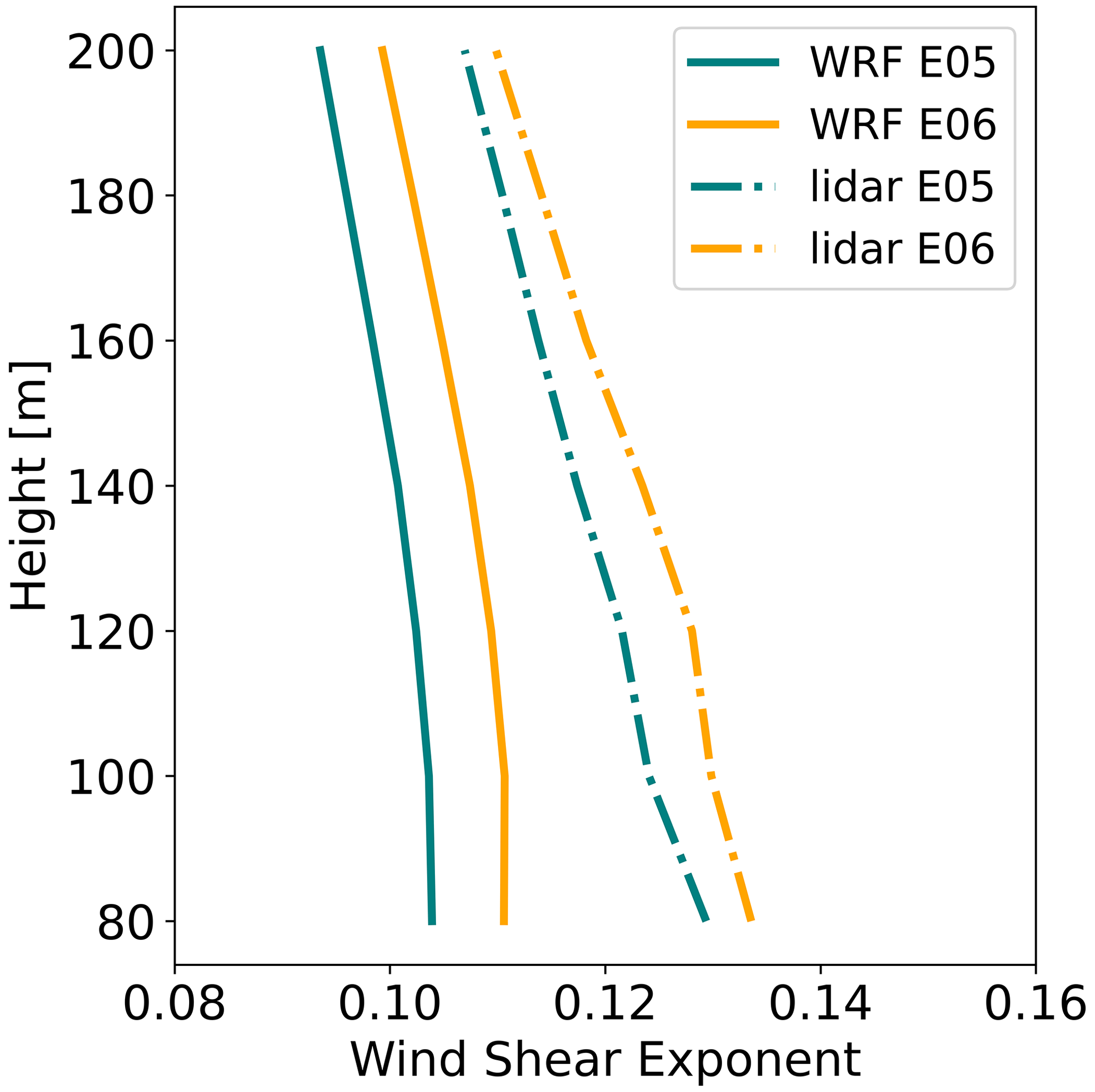
Figure 8Mean wind speed shear exponent by height from NWF (solid) and from lidar measurements (dashed) from 1 September 2019 to 1 September 2020. E05 is shown in blue, and E06 is shown in orange.
Wind speed shear exponents (Eq. 11) differ between NWF and the lidar measurements. The average exponents from lidars E05 and E06 are 0.117 and 0.122, respectively, and are in good agreement with the annual average of 0.12 for both measured and modeled results in the mid-Atlantic (Viselli et al., 2018). The average exponents from WRF at grid cells housing E05 and E06 are 0.099 and 0.106, respectively. NWF-derived exponents correctly capture a decrease with height and lower coefficients at the E05 lidar. However, the exponents are smaller than those calculated from lidar measurements by −0.018 and −0.016 at E05 and E06, respectively. Smaller exponents in NWF may result from overestimated mixing or misrepresentation of wave-induced roughness.
We calculate profiles of the Perkins skill score (PSS) (Perkins et al., 2007) between NWF and lidar wind speeds. Wind speeds are considered at 20 m height intervals from 20 to 200 m. Each wind speed time series is subset by all time stamps with unstable, stable, and neutral stratification. After subsetting, time stamps where lidar observations return NaN are removed from both lidar and NWF time series. At each height, the probability distribution functions of wind speeds are binned at 0.2 m s−1 intervals and normalized such that the frequencies add to unity. The minimum frequency between modeled and observed values for each bin is stored, and the resulting stored values are summed to calculate the following score:
where n is the number of bins, C is the count of normalized values in a bin, and z is the height. A PSS of 1.0 suggests perfect overlap of the two distributions.
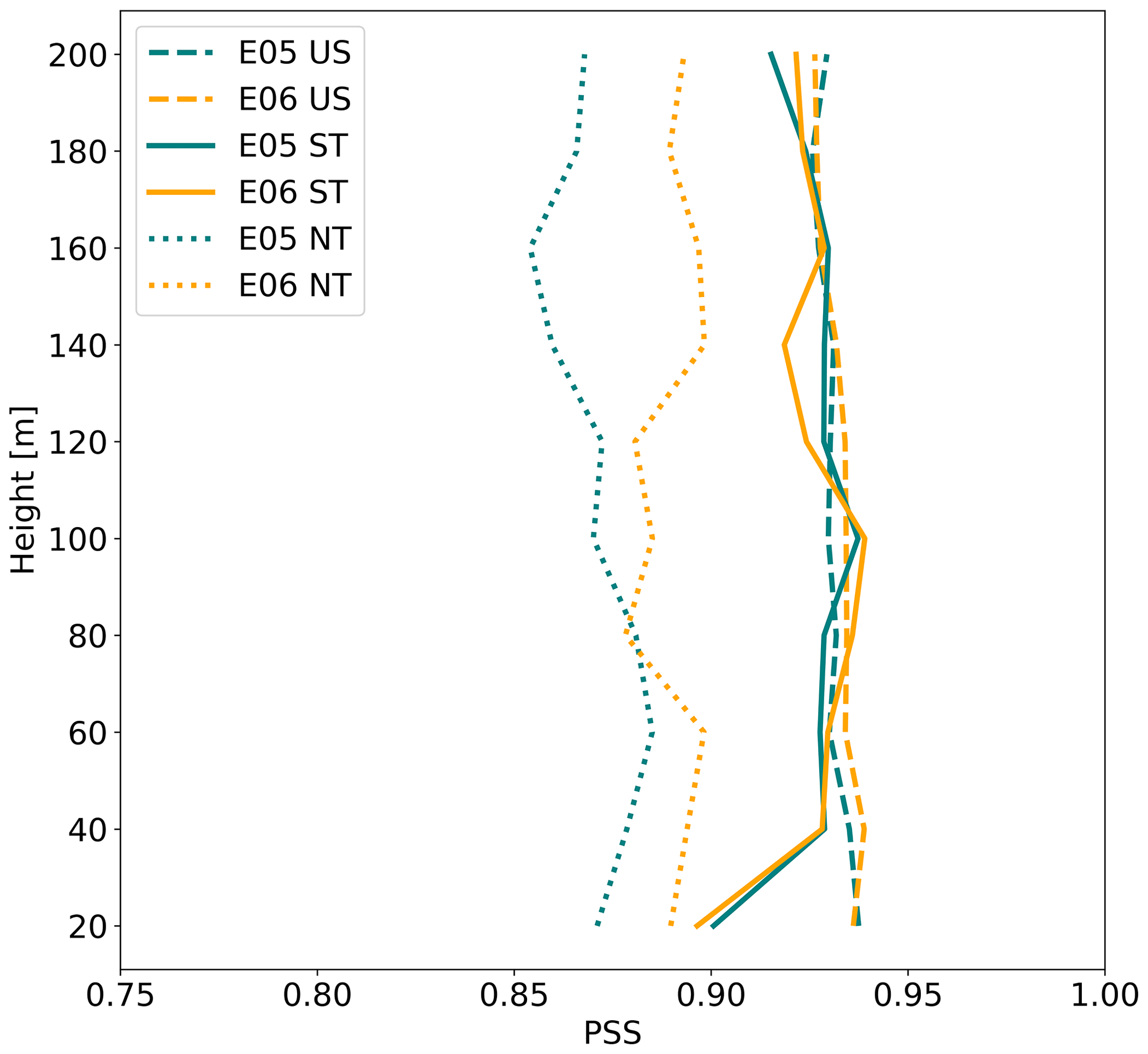
Figure 9Vertical profiles of the Perkins skill score by stratification at the E05 (teal) and E06 (orange) lidars subset by stratification (US – unstable, ST – stable, NT – neutral).
Profiles of PSS (Eq. 12) between NWF and lidar observations of wind speed vary by location and stratification. Performance is generally best in unstable conditions at both E05 and E06 lidar locations with a mean value of 0.93. Performance is the second best in stable conditions, starting around 0.90 at the surface and increasing to 0.93 at 120 m at E05. At E06 in stable conditions, PSS reaches a maximum value of 0.93 at 100 m. Neutral conditions exhibit worse PSS and larger spread by location. AT E05, PSS minimizes at 0.85 at 160 m and maximizes around 0.88 at 60 m. At E06, PSS scores minimize at 0.87 at 80 m and maximize at 0.89 at 140 m.
2.8 Wake identification
The wake delineates the region downwind of turbines with a velocity deficit and turbulence enhancement. We identify the wind speed wake deficit by subtracting NWF wind speeds from WFP wind speeds at the hub height. Averaging across all times during the 1 September 2019 to 1 September 2020 period identifies the overall mean wake wind speed. Because wakes typically propagate to the northeast during stable conditions (Fig. 3), we calculate the propagation distance of wakes along a line extending northeast of the RIMA block (Fig. 1) and report the distance along the line where wake wind speeds reach a threshold. In unstable conditions the prevailing wind direction is northwesterly (Fig. 3), so we assess the wake propagation distance to the southeast instead. The threshold of −0.5 m s−1 is chosen following Golbazi et al. (2022) and Rybchuk et al. (2022). Finally, we define the areal extent of wakes as the area with a wind speed deficit less than −0.5 m s−1.
2.9 Grid balancing
We compare model output energy production to New England grid demand. Demand data are provided hourly (NEISO, 2019). For comparison, we compute hourly averages of WFP power production from each set of simulations. We compare those averages to the national energy supply by acquiring the total from the U.S. Energy Information Administration (EIA, 2023).
2.10 Power variability
Assessing power variability is essential for addressing temporally changing grid demands. We assess the differences in electricity generation for each deployment scenario by separately collecting power output from grid cells containing wind turbines from ONE, LA, and CA simulations. Power is summed across grid cells containing turbines and averaged at 1, 7, and 30 d intervals for comparison. We address seasonal and diurnal variability by further separating and averaging power production totals at each time step into bins by month and hour of day. Power losses from the total, internal, and external wake effects are calculated from the following:
where PLA,CA is the power production at ONE grid cells in the presence of wakes by either the LA or the CA, PONE is the power production in the presence of internal wakes from ONE, and PNWF is the power production from coupling hub-height wind speeds to the power curve. These methods are performed separately by added TKE amount. We note that the upwind conditions change in a LA or CA scenario due to external wakes, which can modify the internal losses in the numerator of Eq. (15). Thus, we provide an alternative method for calculating the external power losses as the difference between the total losses and the internal losses in Eq. (16).
Cluster-induced power deficits at ONE occur due to external wakes from the upwind lease and call areas. Power output from ONE, LA, and CA simulations are averaged in hourly windows at grid cells containing ONE turbines to reduce the effects of numerical noise (Appendix F). The resulting power averages from LA and CA simulations are divided by the averages from ONE at each time stamp. The hour of day and month of year categorize each time stamp, and percentages are placed into bins accordingly. Within each bin the percentages are averaged. Only power production totals greater than 9.9 MW are considered when calculating power losses. This threshold represents the power production total when all turbines within ONE begin operating at the cut-in wind speed. For reference, the total power production for ONE at rated power is 2124 MW. This method is repeated separately for TKE_0 and TKE_100 runs.
Individual wind turbines generate internal wakes within the ONE plant that adversely affect power production. To quantify internal wake effects at ONE, we collect NWF wind speeds at the hub height in each cell containing ONE turbines. Wind speeds are convolved with the power curve and scaled by the number of turbines per cell at 0.01 m s−1 intervals. This method returns the amount of power that ONE would produce in the absence of wakes. Hourly power averages are obtained from both NWF and ONE runs and considered only if power production exceeds 9.9 MW. ONE power totals are divided by the NWF power estimations from the power curve. Again, each time stamp is categorized by hour of day and month of year, and percentages are binned for averaging. These steps are repeated for both TKE_0 and TKE_100 runs.
3.1 Year-round NWF stratification
The predominance of NWF stability conditions changes throughout the year (Figs. 10, 11) as assessed using the Obukhov length (Eq. 5) centered on the RIMA block.
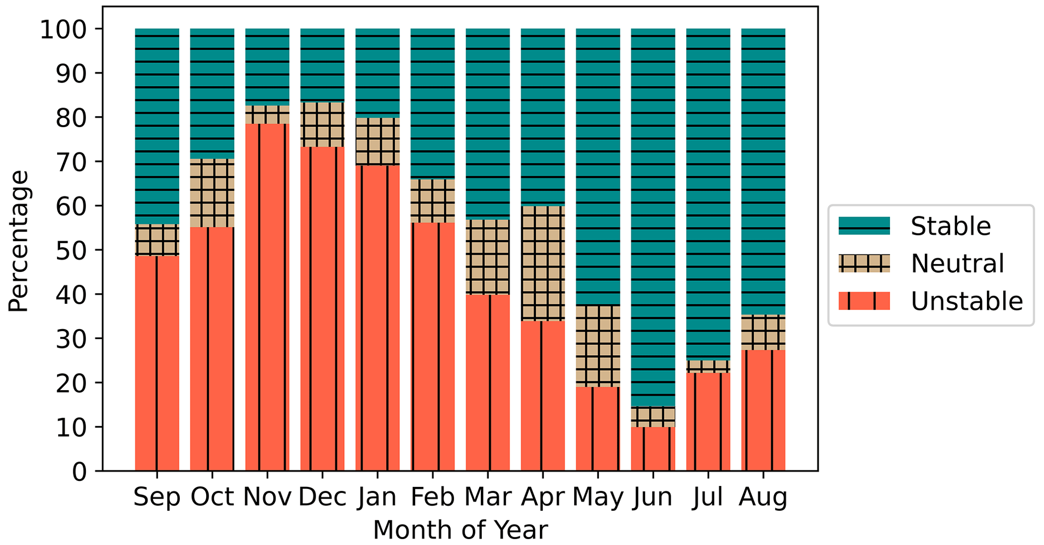
Figure 10Stability classification using the Obukhov length for the 1 September 2019 to 1 September 2020 period at the RIMA block from NWF. The tan crosshatch represents neutral stratification, teal horizontal lines are stable stratification, and red vertical lines are unstable stratification.
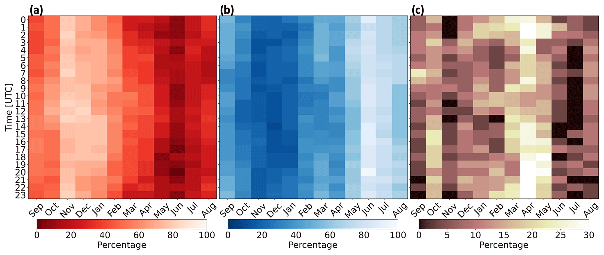
Figure 11Percentages of occurrence for (a) unstable stratification, (b) stable stratification, and (c) neutral stratification from 1 September 2019 to 1 September 2020.
The winter features predominant unstable stratification, whereas the summer features frequent stable stratification (Bodini et al., 2019; Optis et al., 2020) (Figs. 10, 11). The strong stability in summer is caused by nearby surface-heated air advecting over the colder OCS. These dynamics reverse during winter when cold air from land advects over warmer water. Overall, stratification is most frequently unstable during November and stable during June. April features the greatest percentage of neutral conditions as the springtime transition from cooler to warmer air reduces the air–sea temperature gradient. The same pattern occurs elsewhere throughout the OCS because diurnal variability in stratification is weaker than the seasonal cycle (Fig. 11). The mean unstable, stable, and neutral percentages of occurrence at the RIMA block are 44.3 %, 44.4 %, and 11.2 %, respectively, for the 1 September 2019 to 1 September 2020 period. Stability calculations from the model grid cells that house lidars E05 and E06 reveal similar results (Fig. B1). However, L may not always represent conditions aloft (Fig. C1).
3.2 Wake variability
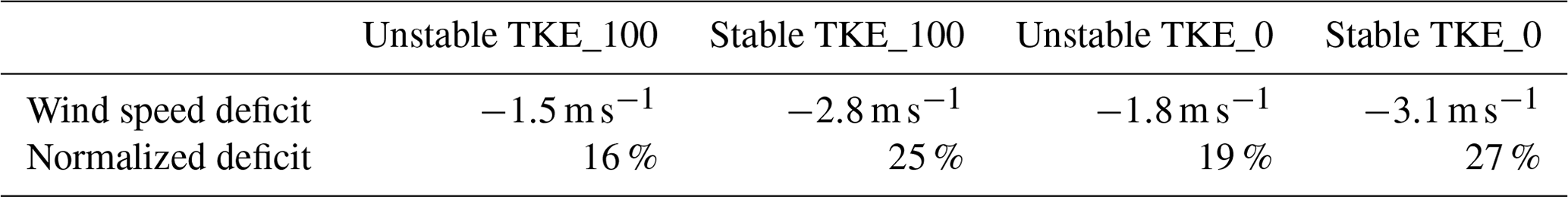
Here, we categorize wakes by the maximum wind speed deficit in space, the spatial extent, and the downwind propagation distance. While wakes remain relatively unchanged between TKE_0 and TKE_100, they drastically vary by stratification. The maximum average wake wind speed deficit occurs within the wind plant areas and intensifies from −1.5 to −2.8 m s−1, moving from unstable to stable conditions for TKE_100 (Fig. 12a, c). Normalized with mean NWF hub-height wind speeds of 9.2 m s−1 (unstable) and 11.2 m s−1 (stable), the corresponding mean wind speed deficits are 16 % and 25 %. Similarly, the maximum average wind speed deficit intensifies from −1.8 to −3.1 m s−1, a normalized reduction of 19 % and 27 %, moving from unstable to stable at TKE_0 (Fig. 12b, d). Thus, reducing TKE from 100 % to 0 % has a smaller impact on wake strength than increasing stability.
Table 3Wake wind speed reduction by stratification and TKE amount.
The areal extent of wakes changes by stability and added TKE. Wake deficits stronger than the −0.5 m s−1 cutoff in unstable stratification at TKE_100 (Fig. 12a) cover a total area of 7208 km2 and represent the best-case scenario where wakes impact the smallest area. In stable stratification at TKE_100 (Fig. 12c), wakes cover a larger area of 15 948 km2, or 2.2 times larger. A similar increase occurs using TKE_0, although areal coverage of the wake is larger due to weaker turbulence-induced wind speed replenishment from aloft. At TKE_0 in unstable conditions (Fig. 12b), wakes stronger than −0.5 m s−1 cover an area of 7780 km2. In stable stratification, the area increases to 15 636 km2 (Fig. 12d), a factor of 2. The spatial extent of strong wakes spreading furthest throughout the region, representing the worst-case scenario, occurs in stable conditions at TKE_100. Wakes interact between immediate wind plant neighbors for all scenarios.
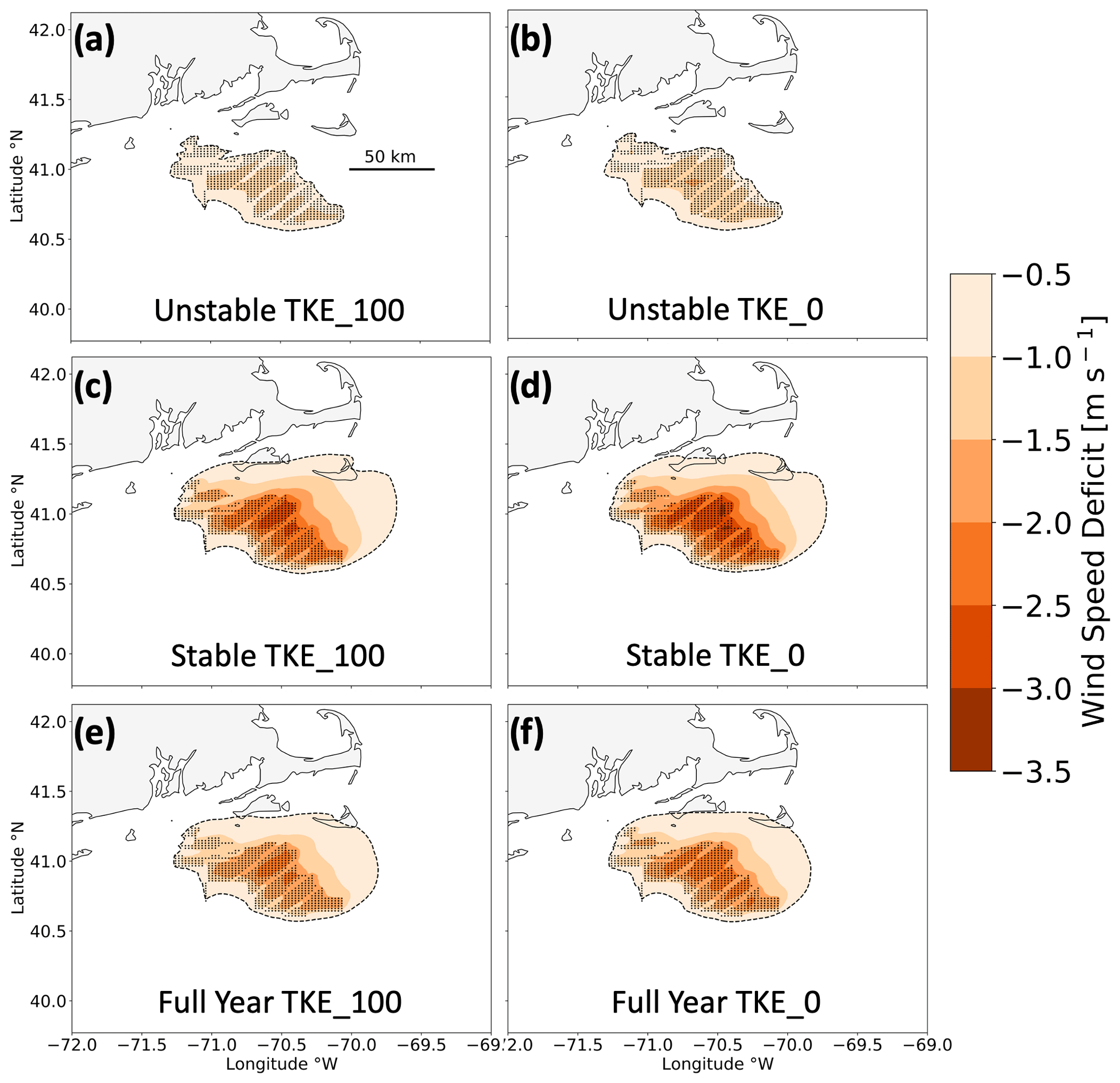
Figure 12Average wake wind speeds among the lease areas during (a, b) unstable stratification, (c, d) stable stratification, and (e, f) the full 1 September 2019 to 1 September 2020 period. Wakes are simulated with 100 % added TKE (a, c, e) or 0 % added TKE (b, d, f). Wind speed deficits are shown by the colored contouring, and turbines are shown as the black dots. The −0.5 m s−1 threshold is outlined by the dashed black line.
Stratification exerts a stronger effect on wake propagation distance than TKE does. For instance, wakes extending 3.7 km downwind in unstable conditions reach 55.4 km in stable conditions at TKE_100 (Fig. 12a, c), similar to the estimate of 50 km from Golbazi et al. (2022). Likewise, wake deficits reaching 5.9 km downwind in unstable stratification reach 55.4 km downwind in stable stratification at TKE_0 (Fig. 12b, d). The same pattern exists for CA wakes (Fig. D1). Overall, altering the added TKE amount has a small impact on the propagation distance of wakes relative to stratification, and combining stable stratification with TKE_0 results in the strongest wakes.
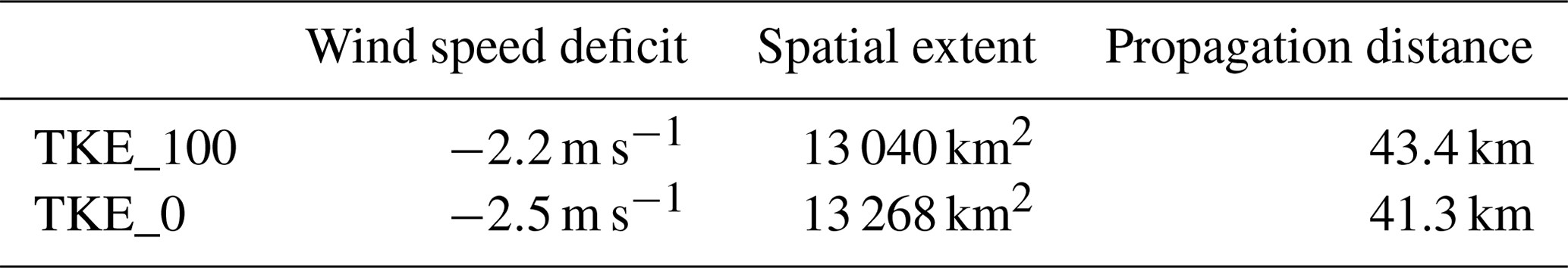
Yearly averaged wakes show similar trends with TKE and stability (Table 4). The maximum wake strength intensifies from −2.2 to −2.5 m s−1 moving from TKE_100 to TKE_0 (Fig. 12e, f). Reducing TKE also increases the spatial coverage of wakes from 13 040 km2 using TKE_100 (Fig. 12e) to 13 268 km2 using TKE_0 (Fig. 12f). Downwind propagation distances remain similar over the yearlong period with wakes reaching 43.4 km at TKE_100 and 41.3 km at TKE_0.
Table 4The wake wind speed deficit, spatial extent, and downwind propagation distance by added TKE amount.
Reduced TKE limits turbulence-induced momentum transport from aloft, thereby increasing wake strength. Counterintuitively, longer-lasting wakes in TKE_100 develop from a larger reduction in momentum from wake recovery above the turbines (Fitch et al., 2012; Siedersleben et al., 2020), leaving less momentum available for replenishment downwind.
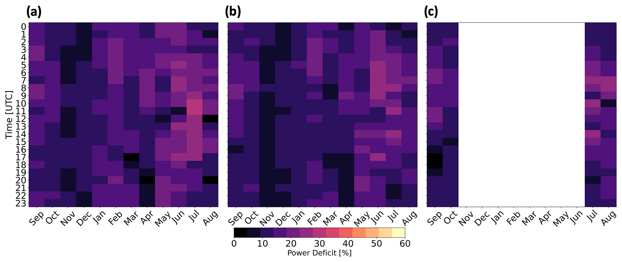
Figure 13The power deficit at ONE when waked by (a) the LA at TKE_0, (b) the LA at TKE_100, and (c) the CA at TKE_100. The white space reflects the simulation period. The color bar is broad to facilitate comparison with losses in Fig. 14.
3.3 Power deficits
3.3.1 External wake losses
ONE experiences power deficits due to external wakes from the LA and the CA. Considering external wakes from the LA at TKE_0 (Eq. 15), the average yearlong power deficit at ONE is 14.7 % (Fig. 13a) and increases to 15.7 % considering only the 4 stable CA months. When ONE is waked by the LA at TKE_100, the average yearlong power deficit reduces to 13.4 % (Fig. 13b) because increased turbulence supports faster replenishment. During the 4 months only, the deficit is 14.4 %. When incorporating wakes from the CA (at TKE_100), the mean ONE power deficit (over 4 months) is 14.3 % (Fig. 13c). By calculating the external power losses as the difference between total and internal losses (Eq. 16) instead, the deficits are 8.97 % and 8.43 % for the LA at TKE_0 and TKE_100, respectively. However, power losses vary as larger reductions from external wakes occur during summer, whereas smaller reductions occur during winter.
External wake-induced losses vary both diurnally and seasonally. Larger power deficits occur more often during summer due to stable stratification (Figs. 10, 11a). Smaller power deficits occur during winter (Fig. 13), with faster winds that exceed rated wind speed and unstable conditions that erode wakes faster. Larger power deficits correspond with stable stratification in June and July. Conversely, smaller power deficits occur with unstable stratification throughout November and December. These patterns occur because colder air advects over warmer water in winter, which causes unstable conditions that erode wakes faster. Conversely, warmer air advects over colder water during the summer, inducing stable conditions that limit turbulent wake recovery. While wake-induced losses vary somewhat across the diurnal cycle, there is no discernible pattern. The ocean's large heat capacity suppresses daytime heating, which limits changes in stratification and, by extension, the magnitude of changes in wake losses.
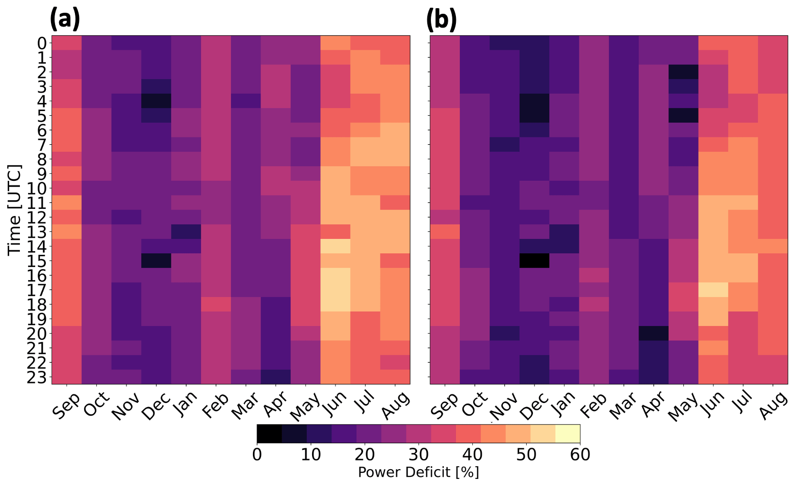
Figure 14The percentage of power loss at ONE from internal wakes at (a) TKE_0 and (b) TKE_100.
3.3.2 Internal wake losses
Internal power deficits (Eq. 14) at ONE are at least 25 % stronger than externally induced power deficits but experience similar variability with stability and TKE amount (Fig. 14). Internal waking induces weaker deficits during winter and stronger deficits during summer. As with external wakes, a clear diurnal pattern fails to emerge. Yearlong internal wakes from TKE_0 and TKE_100 induce power losses of 29.2 % and 25.7 %, respectively. During the 4 stable months only, the deficits increase to 36.9 % and 32.9 %, respectively. Using different PBL schemes with similar turbine spacing under steady-state idealized conditions, Rybchuk et al. (2022) find similar internal losses to capacity factor, up to 31.6 %.
The average yearlong power deficits (Eq. 13) at ONE considering internal wakes and external wakes from the LA range between 38.2 % (TKE_0) and 34.1 % (TKE_100). These results concur with wake-induced losses found by Pryor et al. (2021) of 35.3 % among the LA, based on 11 periods of different flow scenarios spanning 5 d. Observations of wake-induced power losses have large variability over the year, ranging from as low as 5 % to as high as 40 % (Lee and Fields, 2021). Overall, external wakes produce yearly averaged power losses of 14.1 %, whereas internal wakes induce larger losses of 27.4 %. Thus, we stress the importance of resolving region-specific and time-varying wakes for accurate energy prediction estimates.
3.4 Annual energy production
Predictions of energy supply are critical for planning, operations, and diversification of renewables. Without internal or external wake effects, ONE would produce 11.61 TW h and meet 10.02 % of New England's average demand. Annual energy production (AEP) from ONE, considering just internal wakes, reduces to 9.19 TW h (TKE_0) or 9.55 TW h (TKE_100), which could meet 7.94 % to 8.24 % of New England's demand. Including both internal and external wakes from the LA, ONE would produce 8.19 TW h (TKE_0) or 8.65 TW h (TKE_100), meeting 7.07 % to 7.47 % of demand.
Increasing the number of wind turbines increases the demand fulfilled; AEP from the LA is 68.12 TW h (TKE_0) or 70.9 TW h (TKE_100), supplying 58.82 % to 61.22 % of New England's demand. On an hourly basis, the LAs fulfill demand only 24.6 % (TKE_0) and 26.5 % (TKE_100) of the time, highlighting the necessity for resolving accurate wake losses across the OCS. Previous work (Livingston and Lundquist, 2020) assuming a constant 20 % wake loss, shown here to be underestimated, has suggested that 2000 turbines of 10 MW could meet New England's demand 37 % of the time. All in all, the LA, with 1418 turbines of 12 MW, supplies 68 and 71 TW h yr−1, or 1.72 % (TKE_0) to 1.65 % (TKE_100) of the nation's energy supply.
3.5 Power variability by TKE amount
3.5.1 Temporal power variability
While differences in wake strength between TKE amounts alter power production, wind speed exerts a larger influence. Maximum power is produced during spring with the least amount of power produced during summer (Fig. 15a) for both TKE_0 and TKE_100 because spring features faster wind speeds (Fig. 15b). Power production responds to hub-height wind speeds (Fig. 15) more than stability conditions (Figs. 10, 11). Reduced power production during summer may be problematic as New England's top-10 utility demand days since 1997 have all occurred in July or August (NEISO, 2023).
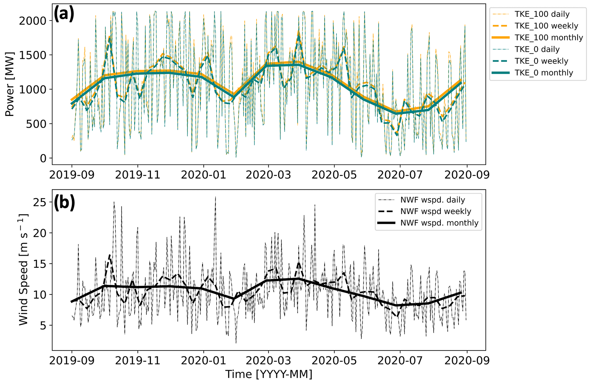
Figure 15(a) Total power production at ONE by TKE amount. TKE_100 power output is shown in orange and TKE_0 output in teal. (b) Hub-height NWF wind speed at a point centered on the RIMA block. The dotted lines represent the daily average, dashed lines the 7 d average, and solid lines the 30 d average.
Total power production varies slightly between TKE_100 and TKE_0. Due to weaker replenishment within the rotor-swept area, TKE_0 wakes are stronger, so TKE_0 produces less total power than TKE_100 (Fig. 15a). Over the year, TKE_0 runs produce 96.2 % (ONE) and 96.1 % (LA) of the power of TKE_100. This difference does not arise from extreme outliers, as TKE_0 runs produce less power more frequently, at 71.3 % (ONE) or 81.2 % (LA) of the time.
3.5.2 Power variability by wind speed
Differences in power production (TKE_100 − TKE_0) vary by NWF hub-height wind speed (Fig. 16). These differences are small at slow wind speeds because little momentum is available for wake recovery and at faster wind speeds within region 3 of the power curve (11–30 m s−1) where wind speed changes do not affect power production (Fig. 2a). Differences in wind speed within region 3 should have no effect on power production and are caused by numerical noise propagating through wind plant areas (Fig. F1). The largest differences in power production occur in region 2 and around rated wind speed where the power curve is steep (Figs. 2a, 16). Additionally, large differences in power production can occur in specific meteorological conditions such as frontal propagation.
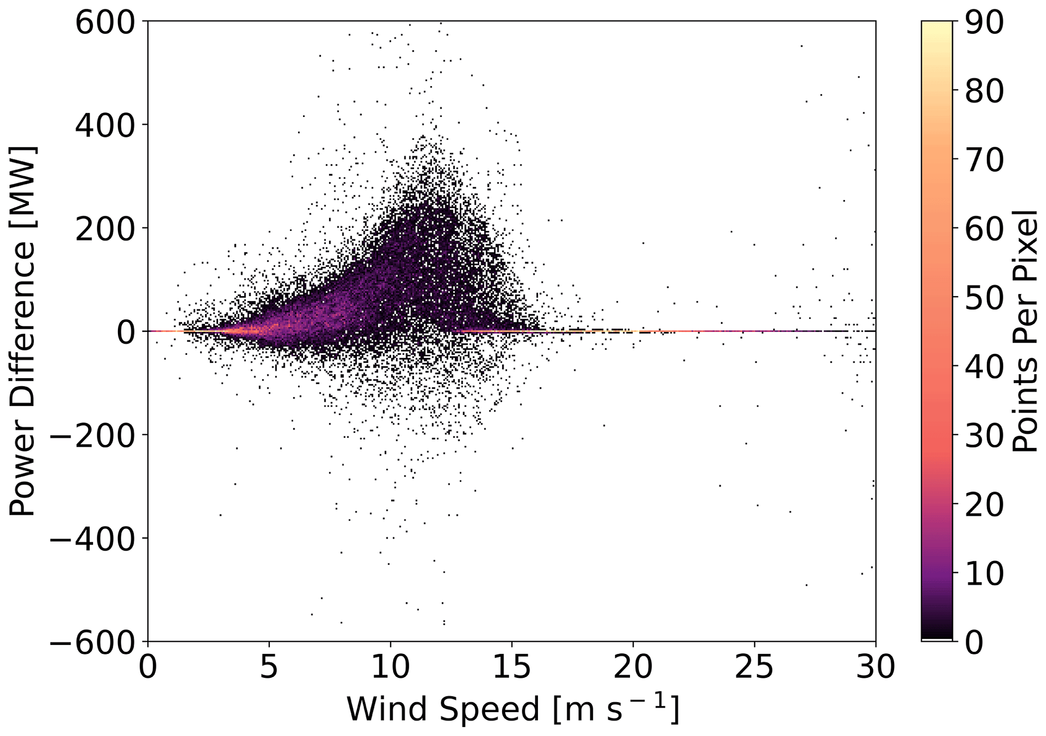
Figure 16The difference in power production (TKE_100-TKE_0) at ONE as a function of wind speed. The colored contouring depicts the density of scattered points per pixel. Wind speeds are obtained every 10 m from a point centered on ONE at hub height.
Comparison of power production between TKE amounts by other meteorological variables lacked significant trends. For example, we additionally analyzed differences in power production by wind direction, following the hypothesis that northerly wind directions could transport more turbulence offshore because land has a higher roughness length than the ocean. TKE_100 runs may harness this mechanical turbulence more for wake replenishment. Analysis of differences in power production by PBL height also failed to show significant patterns. We assumed that higher PBL heights indicated a greater reservoir of turbulence from which TKE_100 runs could replenish the wake, resulting in greater power production. Further analysis concluded by comparing power differences with the aforementioned variables' rates of change. However, we reached the same conclusions, as higher densities of scattered points existed around frequently occurring conditions such as southwesterly wind directions.
Wake strength varies spatiotemporally between TKE_0 and TKE_100 runs. While the mean difference in wind speed at hub height between TKE_100 and TKE_0 runs indicates that TKE_0 produces stronger wakes, this averaging may obscure the actual spatiotemporal variability. For example, a wind plant may have greater TKE_100 wake wind speeds, while its nearby neighbor has greater TKE_0 wake wind speeds at the same point in time. Additionally, a specific wind plant may not consistently produce stronger wakes under one TKE setting. A wind plant may fluctuate between producing stronger wakes in TKE_100 runs and TKE_0 runs throughout time. This finding suggests that other boundary layer dynamics play a role in wake strength, and the variability of power production must be explored.
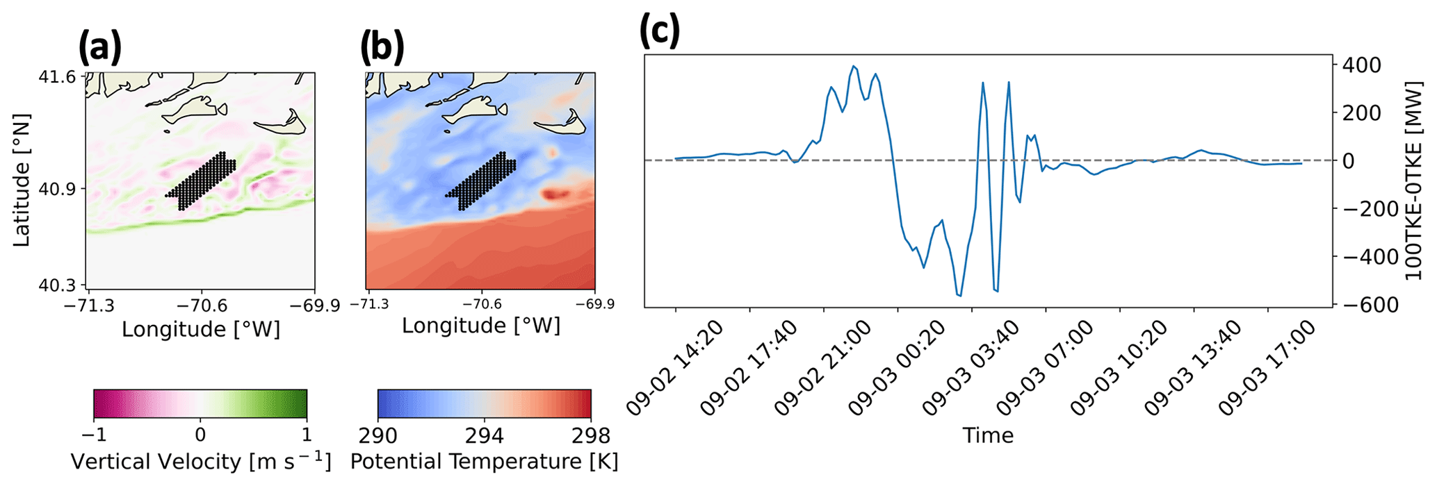
Figure 17Propagation of a cold front through the ONE wind plant. (a) NWF vertical wind speed is shown as the colored contour with upward vertical velocities in greens and downward vertical velocities in purples. (b) NWF potential temperature is shown with lower temperatures in blues and higher temperatures in reds. In both (a) and (b), the black dots indicate wind turbine locations in ONE TKE_0 and TKE_100. (c) The difference in power production between TKE_100 and TKE_0 is shown in MW, with positive values indicating that TKE_100 produces more power.
We note that wind speed and numerical noise are not the only contributors to power differences. One case study analysis shows that TKE_0 and TKE_100 separately produce more power within respective 99th percentiles over a short period of time in September (Fig. 17c). Investigation reveals that a cold front propagated through the ONE wind plant from the northwest to the southeast during this period. The cold front is identified by a lenticular band of upward vertical motion at the frontal head followed by turbulent vertical motion (Fig. 17a) in addition to advection of lower potential temperatures (Fig. 17c). As the cold front approaches, more power is produced by the TKE_100 simulation and is within the 99th percentile. When the frontal head first interacts with Vineyard Wind, more power is produced by the TKE_0 simulation and is within the 99th percentile. Conversely, TKE_100 produces more power following the frontal head. Frontal propagation can induce Kelvin–Helmholtz instabilities, the turbulence of which may aid wake recovery by vertically mixing momentum (Jiang, 2021). Increased turbulence in the TKE_100 simulation can harness more downward vertical transport of momentum from Kelvin–Helmholtz instabilities aft of the frontal head, increase wake replenishment, and produce more power.
This modeling study assesses the variability of wake effects across the mid-Atlantic OCS based on yearlong simulations, including a first step towards uncertainty quantification and approaches for distinguishing internal and external wake effects. In addition to a simulation without wind plants (NWF), validated by comparison to floating lidar observations, three wind plant layouts are explored, including a representative wind plant alone (ONE), all lease areas (LA), and the lease areas plus the call areas (CA). Modifying the added TKE amount (TKE_0 or TKE_100) by turbines provides uncertainty quantification in power production estimates.
The OCS is characterized by more frequent unstable stratification during winter and stable stratification during summer (Bodini et al., 2019; Optis et al., 2020; Debnath et al., 2021). In stable conditions, wakes are stronger and propagate further downwind, (Fitch et al., 2013; Vanderwende et al., 2016; Porté-Agel et al., 2020). In the worst-case scenario where downwind wake recovery diminishes during stable stratification, mean wakes propagate 55 km downwind. While wakes may not reach downwind clusters on average, inter-cluster waking occurs intermittently. While TKE_0 produces stronger wakes than TKE_100, the downwind propagation distances do not differ.
Reduced wake wind speeds, as compared to the NWF simulation, affect power production. Yearly averaged wake losses induce power deficits at ONE from 38.2 % (TKE_0) to 34.1 % (TKE_100). This deficit comprises both internal and external waking. External wakes induce yearly averaged power losses of 14.7 % (TKE_0) or 13.4 % (TKE_100), whereas wakes from the CA induce similar losses of 14.3 % over 4 months. Using an alternative method, external wakes induce losses of 8.97 % and 8.43 % for the LA at TKE_0 and TKE_100, respectively. Internal wakes at ONE promote larger power losses of 29.2 % (TKE_0) or 25.7 % (TKE_100). Wake-induced power losses vary seasonally with smaller diurnal variability. Larger power deficits occur during summer, where frequent stable conditions limit wake erosion. Although upwind clusters may generate strong external wakes among the LA, wind plant orientation with respect to prevailing winds can reduce adverse impacts from nearby neighbors. Ample distance for replenishment of external wakes by the CA moderates the negative effects. Internal wake losses remain larger due to shorter distances with limited wake recovery. Both external and internal wake-induced losses grow in summer stably stratified conditions. These losses similarly increase in strength for TKE_0 simulations from inhibited recovery.
Resolving precise wake losses and AEP are crucial for stakeholders and grid operators. In the absence of wakes, ONE could supply 10.02 % of New England's demand. Operating alone, ONE's supply reduces to 7.94 % (TKE_0) or 8.24 % (TKE_100). Adding external wakes from the LA, ONE's annual supply lessens to 7.07 % (TKE_0) or 7.47 % (TKE_100). Although wakes are stronger among the LA, the greater number of turbines can meet 58.82 % (TKE_0) and 61.22 % (TKE_100) of New England's demand, or roughly 1.72 % and 1.65 % of national demand. However, the LA only satisfies demand about 25 % of the time on an hourly basis. Overall, spring features maximum power production with the fastest hub-height wind speeds. Wind speeds are slower in summer, reducing power production during July and August, which have featured New England's top-10 utility demand days since 1997 (NEISO, 2023).
Variable TKE amounts marginally impact power generation. TKE_0 simulations average 3.8 % less production than TKE_100 throughout the year, as reduced turbulence in TKE_0 limits momentum transport into the waked zone. Although differences in power production are small, both simulations exhibit large variability at short temporal periods. Improving WFP accuracy by accounting for wind shear throughout the rotor-swept region (Redfern et al., 2019) and dynamic air density may increase the variability in power production further (Wu et al., 2022). Further, different sizes of turbines may be installed in some of these regions, and the size of the turbine can influence the impacts of the turbine (Golbazi et al., 2022).
Future wind resource assessments may neglect differences between TKE_0 and TKE_100 because the power production offset is minor, although we identify a strong outlier during a frontal passage when differences in power production between TKE_100 and TKE_0 are large. While power production differences are minor, effects on other atmospheric variables may be more significant (Fig. A1). Variability may be influenced by other meteorological conditions. Successive analyses should consider yearlong CA simulations to identify the full range of external wake impacts. Although we infer that the effects of CA wakes on ONE are small relative to LA wakes, yearlong estimates may show otherwise. Notably, we find that internal wakes have larger impacts on power production than those generated externally.
To assess the sensitivity of simulations to the amount of parameterized TKE, we conducted a set of 2 d test runs from 11 to 13 July 2017. This time period was chosen for its predominance of southwesterly winds, which represent typical conditions across the OCS, and for the availability of Air–Sea Interaction Tower lidar observations for wind profile validation of the NWF simulations. Test runs consist of 0 % (TKE_0), 25 % (TKE_25), 50 % (TKE_50), and 100 % (TKE_100) added TKE with the WFP.
Hub-height wind speeds vary by simulation type and added TKE amount (Fig. A1a). Mean WFP wind speeds are always slower than NWF wind speeds due to the momentum sink introduced by wind turbines, by 2.9 m s−1. Larger variations between wind speeds (Fig. A1a) correspond with larger spreads in power output by TKE amount (Fig. A1c). The sequencing of power production driven by TKE amount remains consistent, namely that the differences progress from TKE_0 to TKE_25, TKE_50, TKE_75, and TKE_100. Because power production totals for TKE_25 and TKE_50 are typically bounded by the totals for TKE_0 and TKE_100, production simulations incorporate TKE_0 and TKE_100 only to account for the full range of uncertainty throughout a full yearlong period from 1 September 2019 to 1 September 2020.
Although subtle, several important meteorological quantities from the model grid cell at the center of the RIMA block vary by the added TKE amount. For example, wind speeds are slower on 12 July between 12:00 and 16:00 UTC (Fig. A1a). The wind speed reduction during this time period causes a corresponding decrease in turbulent transport of moisture. The mean difference in moisture fluxes throughout the full period between TKE_100 and TKE_0 is kg m−2 s−1 (Fig. A1b). Note that the surface moisture flux remains negative throughout the period. While maritime moisture profiles typically exhibit a decrease in concentration with height, corresponding with a positive flux, mixing from the turbines reduces the near-surface concentration and reverses the gradient.
Heat flux exhibits large variability. The mean difference in heat flux throughout the full period between TKE_100 and TKE_0 is 3.61 W m−2 (Fig. A1d). The wind speed decrease between 12:00 and 16:00 UTC reduces surface stresses and turbulent transport of heat. The reduction in heat flux during this time period causes 2 m temperatures to decrease and exhibit less variability by TKE amount, with a mean difference of 0.26 K between TKE_100 and TKE_0 (Fig. A1f).
The reduction in turbulent mixing lowers the PBL, regardless of TKE amount, to shallow heights between 30 to 80 m at 13:00 UTC (Fig. A1e). The near-surface PBL height suppresses the small variations in turbulent mixing across test runs and causes fluxes to equalize. PBL heights differ the most by added TKE amount and may result from changes in weighting between two separate height determination methods present in the MYNN physics driver (Fig. A1c).
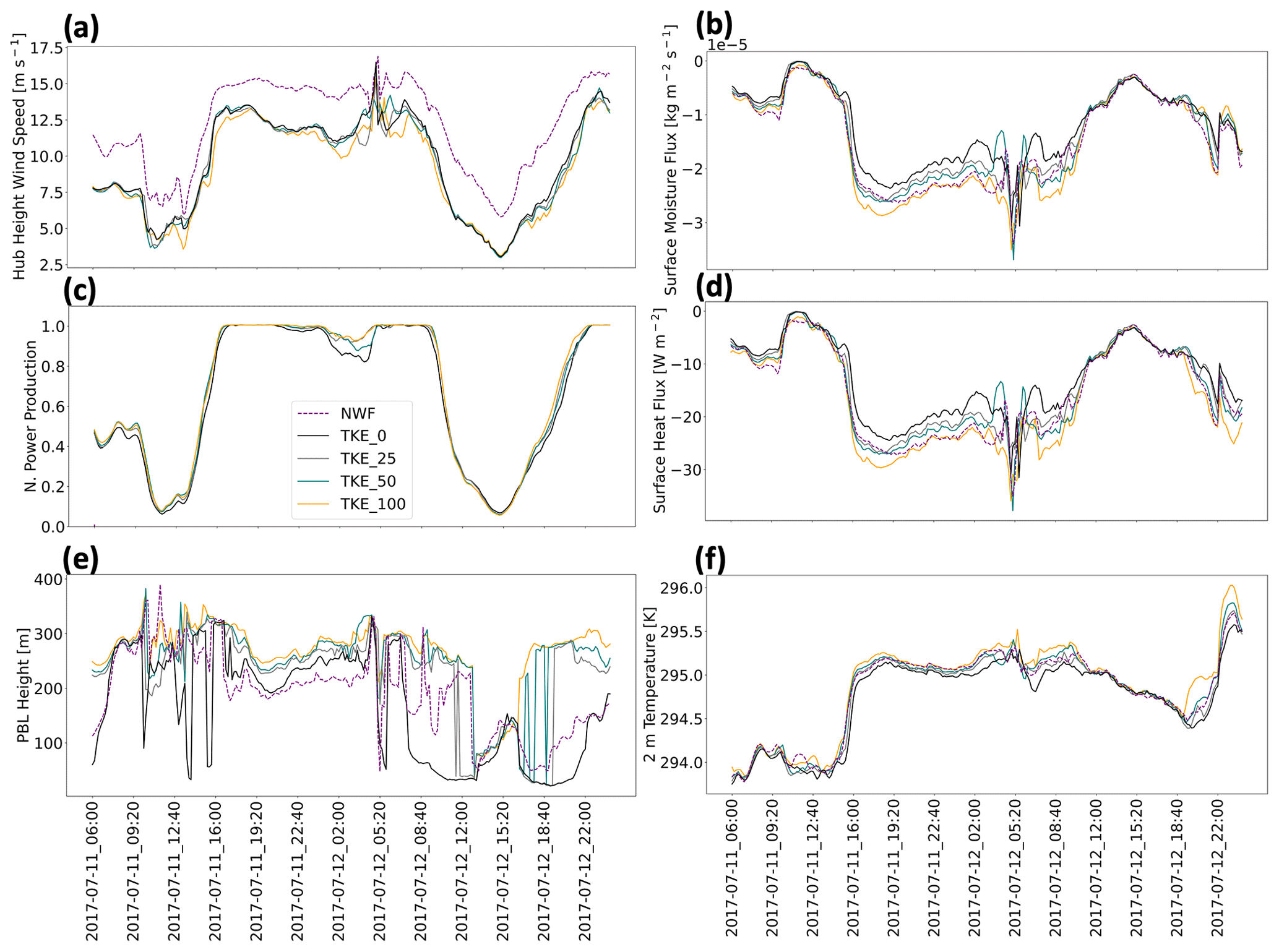
Figure A1The effects of modifying the amount of turbulent kinetic energy (TKE) during test runs. Panels show (a) hub-height wind speed, (b) surface moisture flux, (c) normalized power production, (d) surface heat flux, (e) planetary boundary layer (PBL) height, and (f) 2 m temperature. Values are collected from a point centered on the RIMA block. Power production is the sum of all cells containing wind turbines. TKE_100 is shown in orange, TKE_50 in blue, TKE_25 in gray, TKE_0 in black, and NWF in purple dashes.
Stratification at the E05 and E06 lidars (Fig. B1) exhibits similar seasonal variability to the RIMA block (Fig. 10). The winter months feature predominant unstable stratification caused by cold air advecting over a warm sea surface. In the spring and early summer, stratification transitions to more common stable conditions as warm air advects over a cooler sea surface. Stratification is most commonly unstable in November and stable in May.
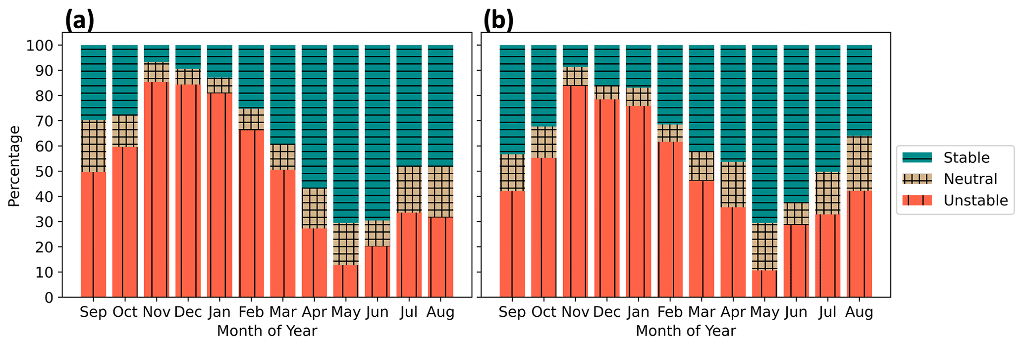
Figure B1Stability classification using the Obukhov length for the 1 September 2019 to 1 September 2020 period at the (a) E05 and (b) E06 lidars from NWF. The tan crosshatches are neutral stratification, blue horizontal bars are stable stratification, and red vertical bars are unstable stratification.
Surface estimates of L may not represent stability aloft (Fig. C1) and may overestimate unstable conditions. When considering monthly averaged potential temperature profiles through the rotor layer, only November and December appear unstably stratified. While September and October appear predominantly unstable based on surface estimates, potential temperature gradients within the rotor-swept area suggest slightly stable conditions, supporting inferences that offshore conditions are stable during late summer. Therefore, our limited set of CA simulations focus on 1 September to 31 October 2019 and 1 July to 31 August 2020 for its presumed abundance of stable stratification.
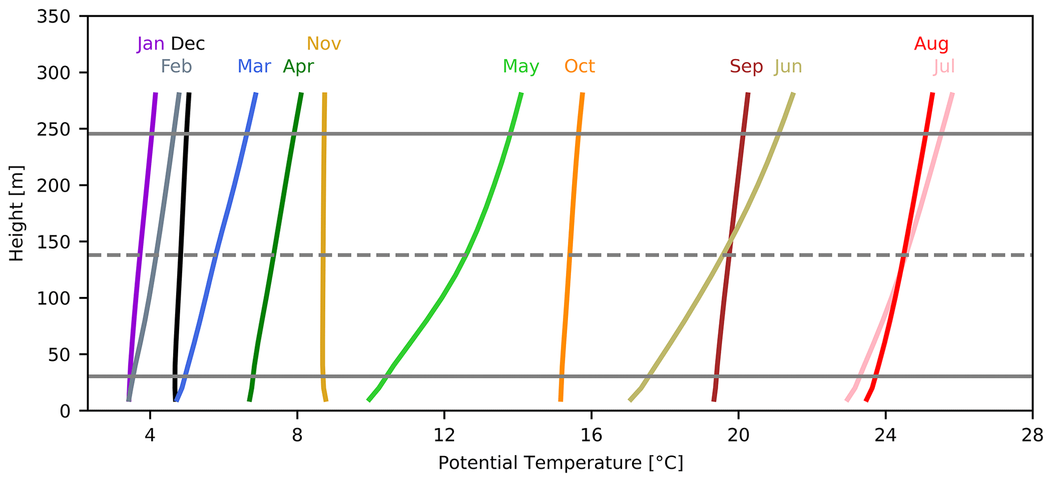
Figure C1Monthly averaged WRF-simulated potential temperature profiles at a point centered on the RIMA block. Horizontal gray lines indicate the levels of the hub height (dashed) and the rotor-swept area (solid).
Wakes in the simulations with CA show similar dependence on stratification (Fig. D1). Note that we simulate the CA for 4 months only (1 September to 31 October 2019 and 1 July to 31 August 2020) at one TKE level only (TKE_100) due to computational costs. The maximum wake strength intensifies from −1.6 to −3.2 m s−1 moving from unstable to stable stratification (Fig. D1b, c).
Wake propagation distance for the call area simulation is also affected by stratification. During the 4 months considered, unstable, stable, and neutral conditions occur 38.2 %, 53.4 %, and 8.3 % of the time, respectively. As such, there is essentially an even split between the percentage of occurrence of unstable and stable conditions. In unstable conditions, wakes from the two southernmost lease areas fail to reach neighboring downwind clusters on average, and no wakes stronger than this threshold reach the RIMA block (Fig. D1e). In stable stratification, wakes from each cluster reach downwind clusters, including the RIMA block (Fig. D1f). Averaged over all 4 months, wakes between LA and the CA along the New Jersey and New York bights affect each other, but no wakes reach the RIMA block. Wakes may still interact with downwind plants at individual times and affect power production.
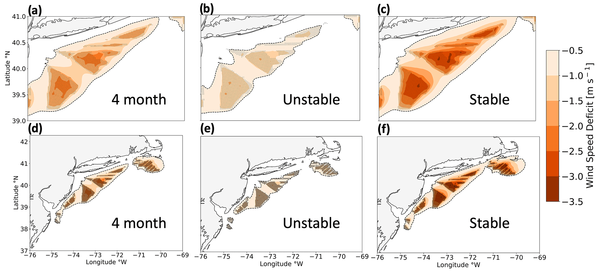
Figure D1Average wake wind speed deficits among the call areas (a, d) for the combined 4-month period, 1 September to 31 October 2019 and 1 July to 31 August 2020, (b, e) during unstable stratification and (c, f) during stable stratification. All panels show 100 % added TKE. Wake wind speed deficits are shown by the colored contour, and turbines are shown as black dots. The upper row is zoomed in to increase granularity.
Here, we characterize the (WFP-NWF) TKE differences by maximum value and by spatial extent. The maximum average TKE additions remain similar by stratification at TKE_100, reaching 1.00, 1.01, and 1.00 m2 s−2 during unstable conditions, stable conditions, and the full year, respectively (Fig. E1a, c, e). The amount of added TKE is not homogeneous across the wind plants in TKE_100, as the greatest contributions occur in grid cells containing more wind turbines. Some TKE is introduced in TKE_0 due to wind speed shear, although the amounts are over an order of magnitude smaller. The maximum average TKE amounts for TKE_0 are 0.05, 0.03, and 0.03 m2 s−2 during unstable conditions, stable conditions, and the full year, respectively. Being purely shear induced, regions experiencing the most TKE in TKE_0 correspond more with the maximum wake wind speed deficits (Fig. 12b, d, f).
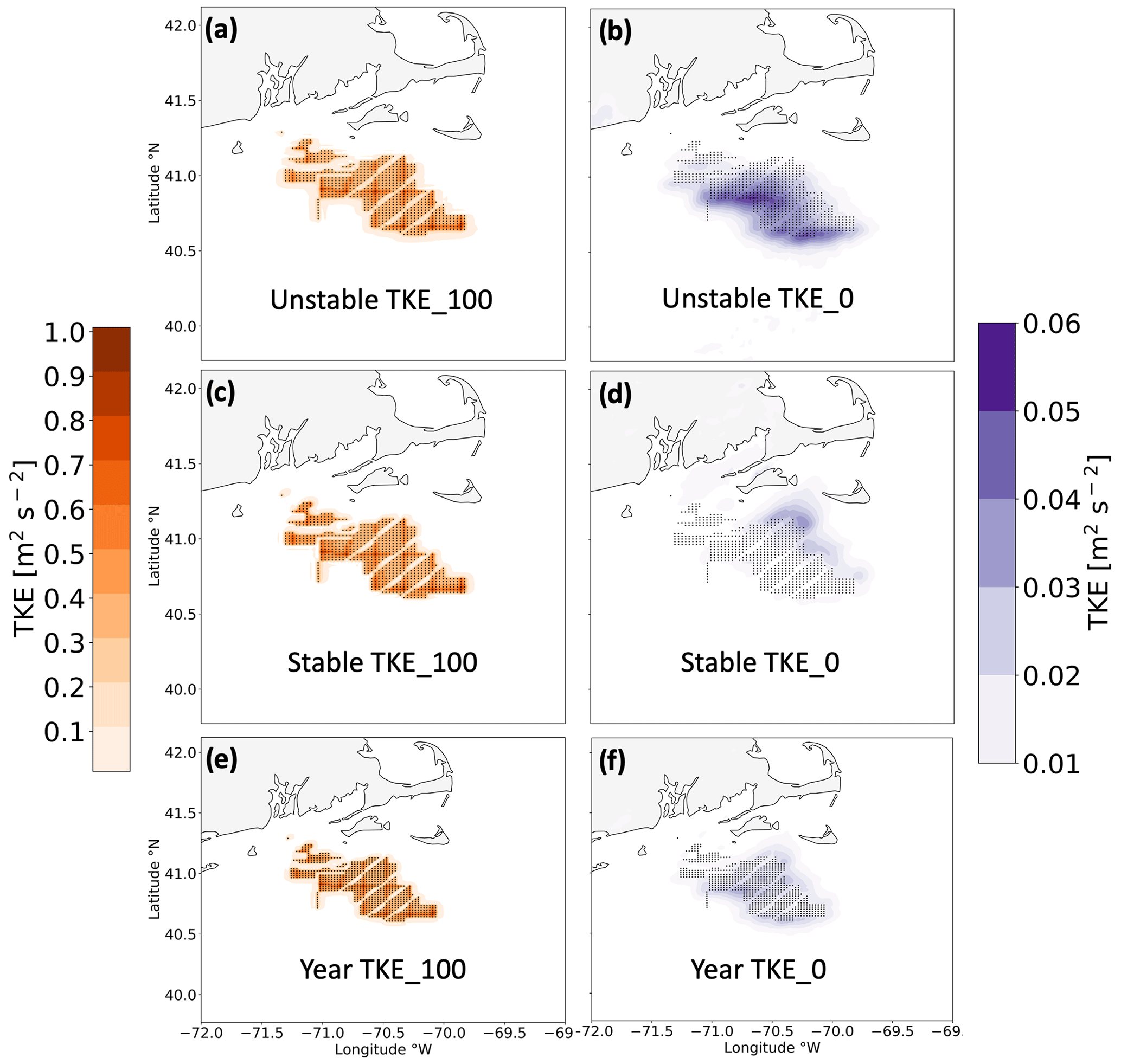
Figure E1Average hub-height (WFP-NWF) TKE difference among the lease areas during (a, b) unstable stratification, (c, d) stable stratification, and (e, f) the full 1 September 2019 to 1 September 2020 period. Panels show 100 % added TKE (a, c, e) or 0 % added TKE (b, d, f). The TKE amount is shown by the colored contouring, and turbines are shown as the black dots.
We further characterize added TKE amounts by their spatial extent. We report the area encompassed by added TKE amounts greater than a threshold of 0.005 m2 s−2 because a cutoff of 0 m2 s−2 includes noise throughout the domain (Fig. F1), and the spatial extent is not realistic. In TKE_100, the spatial extents are 10 724, 10 064, and 9608 km2 in unstable stratification, stable stratification, and for the full year, respectively (Fig. E1a, c, e). In TKE_0, the spatial extents are 13 888, 10 724, and 11 332 km2 in unstable stratification, stable stratification, and for the full year, respectively (Fig. E1b, d, f).
Results can show evidence of numerical noise, which emerges when simulations incorporate the WFP (Ancell et al., 2018; Lauridsen and Ancell, 2018). In our simulations, these brief periods of numerical noise emerge and decay, often coincident with precipitation. While we expect differences in wake wind speed immediately downwind of power plants, it is unlikely that these differences could advect to the southeast corner of the domain, roughly 600 km southeast of the RIMA block (Fig. F1a). If this numerical noise occurred in grid cells with turbines, then this noise would introduce error in power estimations.
We explored several approaches to mitigate the numerical noise, none of which succeeded. First, we increased the floating-point accuracy of numerical calculations by enabling double precision in WRF. Double precision limits the growth of rounding error to smaller magnitudes (Ancell et al., 2018). This attempt aimed to confine perturbations to smaller orders of magnitude that take longer periods of time to become substantial. To prevent “runaway” error growth after long periods of time, we submit simulation restarts each month.
In observing a spatial correlation of numerical noise with convective precipitation during test runs, we reran test simulations with a more complex microphysics scheme. The Thompson microphysics scheme, used throughout, is double moment with respect to cloud ice only. We substituted the Morrison microphysics scheme, which is fully double moment with respect to cloud droplets and rain, cloud ice, snow, and graupel (Morrison et al., 2009). The use of Morrison microphysics did not improve numerical noise, so its computational cost could not be justified.
Next, we introduced a filter for shortwave numerical noise by prohibiting upgradient diffusion. Doing so requires setting the parameter diff_6th_opt to 2 in the namelist, as certain combinations of advection and diffusion orders are conducive to mitigating noise around heavy precipitation (Kusaka et al., 2005). While Kusaka et al. (2005) found the combination of fifth-order advection and sixth-order diffusion to perform best, we had previously attempted this combination because default advection in WRF is fifth order. Thus, we attempted the next best recommendation – combining sixth-order advection and diffusion. Again, this combination did not improve results.
We made a final attempt at noise reduction by running an ensemble of three members using a stochastic kinetic energy backscatter scheme. Ensemble members contain seeds with variable time steps that randomly inject kinetic energy into grid cells (Berner, 2013). These stochastic supplements replenish the kinetic energy sink from unresolvable subgrid-scale processes. We followed recommendations to perturb the stream function and potential temperature backscatter rates by and , respectively. Again, while subtle differences emerged between the simulations, little improvement was found.
We saw little improvement from the aforementioned preprocessing efforts. Given this lack of improvement and a need to conserve computational resources, we employed averaging during postprocessing to alleviate the effects of noise. Modifying averaging periods impacts the range of numerical noise in the wind speed field (Fig. F1b). Noise occurring in grid cells containing turbines could undermine power estimation accuracy, and we observed noise occurring in the southeastern portion of the domain. Subtraction of wind speeds between simulations with variable TKE amounts should only show differences within the wake, and such differences are a result of noise. Averaging periods provide greater relief. While 2 and 4 h averaging periods deliver the best results, these temporal scales can hide important diurnal variability. Conversely, a 30 min averaging period can improve results, but local extrema occasionally reach magnitudes similar to the magnitudes of the raw noise. Thus, hourly averaging can mitigate noise without masking important variability. As a final note, other researchers have benefitted by employing grid nudging within this domain above the PBL (Maryam Golbazi, personal communication, September 2022).
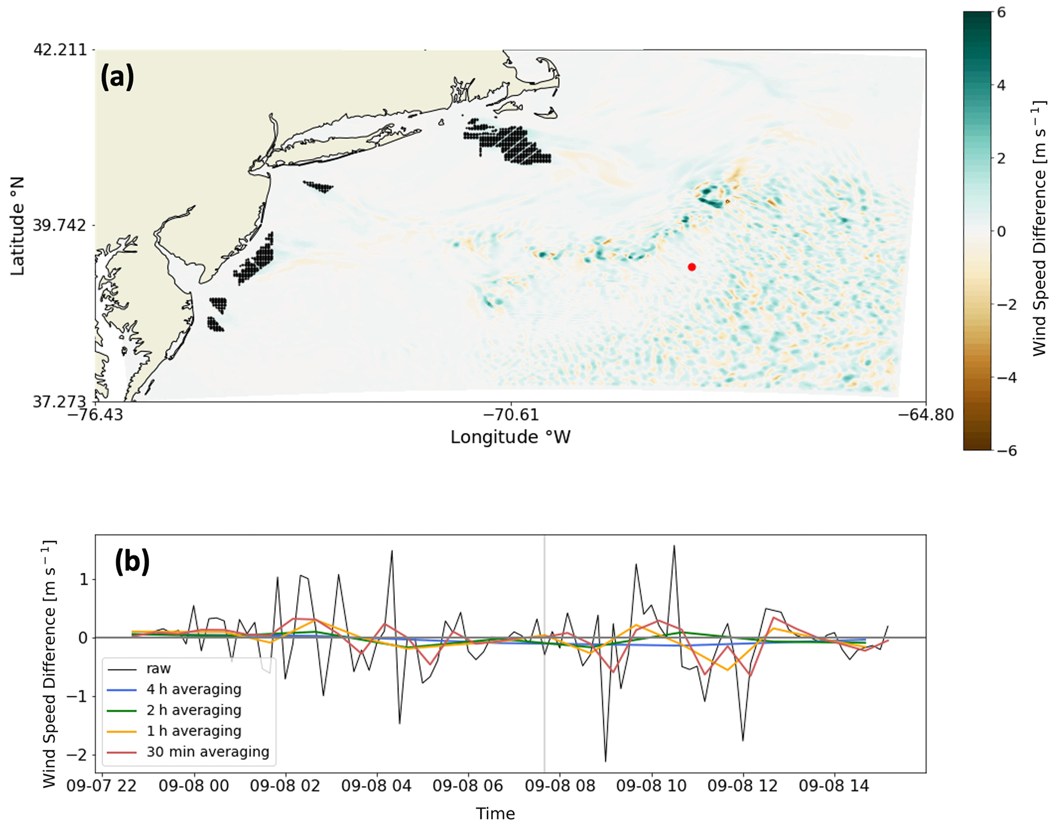
Figure F1(a) The wind speed difference between TKE_100 and TKE_0 at the hub height from LA runs. Wind turbines are shown as black dots. The blue contouring indicates TKE_100 produced faster wind speeds and vice versa. (b) Wind speeds obtained at the red circle in (a) are shown as a time series. The raw difference in wind speeds and averaging periods are shown as different line colors in the time series. The vertical gray line shows the time stamp of the map.
The data and files that support this work are publicly available. The ERA5 boundary conditions can be downloaded from the ECMWF Climate Data Store at https://doi.org/10.24381/cds.bd0915c6 (Hersbach et al., 2023). Shapefiles including the bounding extents of the lease and call areas are available at https://www.boem.gov/renewable-energy/mapping-and-data/renewable-energy-gis-data (Bureau of Ocean Energy Management, 2023). Individual turbine coordinates and their power and thrust curves are provided at https://doi.org/10.5281/zenodo.7374283 (Rosencrans, 2022). WRF namelists for NWF and WFP simulations can be obtained at https://doi.org/10.5281/zenodo.7374239 (Rosencrans, 2021). The simulation output data will be available in HDF5 format at https://doi.org/10.25984/1821404 (National Renewable Energy Laboratory, 2020).
Conceptualization: JKL and MO. Methodology: DR, JKL, and MO. Software: DR, AR, and MR. Validation: DR. Formal analysis: DR. Investigation: DR and JKL. Resources: MO and NB. Writing (original draft): DR and JKL. Writing (review and editing): all co-authors. Visualization: DR. Supervision: JKL, MO, and NB. Project administration: MO and NB. Funding acquisition: MO and NB.
At least one of the (co-)authors is a member of the editorial board of Wind Energy Science. The peer-review process was guided by an independent editor. Furthermore, Mike Optis co-authored the submitted manuscript while he was an employee of the National Renewable Energy Laboratory. He has since founded Veer Renewables, which recently released a wind modeling product, WakeMap, which is based on a similar numerical weather prediction modeling framework as the one described in this paper. Data from WakeMap are sold to wind energy stakeholders for profit. Public content on WakeMap include a website (https://veer.eco/wakemap/, last access: 18 March 2023), a white paper (https://veer.eco/wp-content/uploads/2023/02/WakeMap_White_Paper_Veer_Renewables.pdf, last access: 18 March 2023), and several LinkedIn posts promoting WakeMap. Mike Optis is the founder and president of Veer Renewables, a for-profit consulting company. Mike Optis is a shareholder of Veer Renewables and owns 92 % of its stock.
The views expressed in the article do not necessarily represent the views of the DOE or the U.S. Government. The U.S. Government and the publisher, by accepting the article for publication, acknowledge that the U.S. Government retains a nonexclusive, paid-up, irrevocable, worldwide license to publish or reproduce the published form of this work, or allow others to do so, for U.S. Government purposes. Neither NYSERDA nor OceanTech Services/DNV have reviewed the information contained herein and the opinions in this report do not necessarily reflect those of any of these parties.
Publisher's note: Copernicus Publications remains neutral with regard to jurisdictional claims made in the text, published maps, institutional affiliations, or any other geographical representation in this paper. While Copernicus Publications makes every effort to include appropriate place names, the final responsibility lies with the authors.
This work was supported by an agreement with NREL under APUP UGA-0-41026-125. This work was authored (in part) by the National Renewable Energy Laboratory, operated by the Alliance for Sustainable Energy, LLC, for the US Department of Energy (DOE) under contract no. DE-AC36-08GO28308. A portion of computation used the Blanca condo computing resource at the University of Colorado Boulder. Blanca is jointly funded by computing users and the University of Colorado Boulder. A portion of computation used the Summit supercomputer, which is supported by the National Science Foundation (awards ACI-1532235 and ACI-1532236), the University of Colorado Boulder, and Colorado State University. The Summit supercomputer is a joint effort of the University of Colorado Boulder and Colorado State University. A portion of this research was performed using computational resources sponsored by the DOE's Office of Energy Efficiency and Renewable Energy and located at NREL.
Funding was provided by the US Department of Energy's Office of Energy Efficiency and Renewable Energy and the Wind Energy Technologies Office and by the National Offshore Wind Research and Development Consortium (grant no. CRD-19-16351).
This paper was edited by Andrea Hahmann and reviewed by three anonymous referees.
218th Legislature: NJ Renewable Portfolio Standards, https://pub.njleg.gov/bills/2018/A4000/3723_I1.PDF (last access: 10 August 2022), 2018.
Aitken, M. L., Kosoviæ, B., Mirocha, J. D., and Lundquist, J. K.: Large eddy simulation of wind turbine wake dynamics in the stable boundary layer using the Weather Research and Forecasting Model, J. Renew. Sustain. Ener., 6, 033137, https://doi.org/10.1063/1.4885111, 2014.
Ancell, B. C., Bogusz, A., Lauridsen, M. J., and Nauert, C. J.: Seeding Chaos: The Dire Consequences of Numerical Noise in NWP Perturbation Experiments, B. Am. Meteorol. Soc., 99, 615–628, https://doi.org/10.1175/BAMS-D-17-0129.1, 2018.
Antonini, E. G. A., Romero, D. A., and Amon, C. H.: Optimal design of wind farms in complex terrains using computational fluid dynamics and adjoint methods, Appl. Energ., 261, 114426, https://doi.org/10.1016/j.apenergy.2019.114426, 2020.
Archer, C. L., Colle, B. A., Veron, D. L., Veron, F., and Sienkiewicz, M. J.: On the predominance of unstable atmospheric conditions in the marine boundary layer offshore of the U.S. northeastern coast, J. Geophys. Res.-Atmos., 121, 8869–8885, https://doi.org/10.1002/2016JD024896, 2016.
Archer, C. L., Wu, S., Ma, Y., and Jiménez, P. A.: Two Corrections for Turbulent Kinetic Energy Generated by Wind Farms in the WRF Model, Mon. Weather Rev., 148, 4823–4835, https://doi.org/10.1175/MWR-D-20-0097.1, 2020.
Arthur, R. S., Mirocha, J. D., Marjanovic, N., Hirth, B. D., Schroeder, J. L., Wharton, S., and Chow, F. K.: Multi-Scale Simulation of Wind Farm Performance during a Frontal Passage, Atmosphere, 11, 245, https://doi.org/10.3390/atmos11030245, 2020.
Beiter, P., Musial, W., Duffy, P., Cooperman, A., Shields, M., Heimiller, D., and Optis, M.: The Cost of Floating Offshore Wind Energy in California Between 2019 and 2032, NREL/TP-5000-77384, https://doi.org/10.2172/1710181, 2020.
Berner, J.: WRF Implementation Details and Version history of a Stochastic Kinetic-Energy Backscatter Scheme (SKEBS), National Center for Atmospheric Research Tech. Note, https://www2.mmm.ucar.edu/wrf/users/docs/skebs_in_wrf.pdf (last access: 22 July 2023), 2013.
Bodini, N., Lundquist, J. K., and Kirincich, A.: U.S. East Coast Lidar Measurements Show Offshore Wind Turbines Will Encounter Very Low Atmospheric Turbulence, Geophys. Res. Lett., 46, 5582–5591, https://doi.org/10.1029/2019GL082636, 2019.
Bodini, N., Optis, M., Redfern, S., Rosencrans, D., Rybchuk, A., Lundquist, J. K., Pronk, V., Castagneri, S., Purkayastha, A., Draxl, C., Krishnamurthy, R., Young, E., Roberts, B., Rosenlieb, E., and Musial, W.: The 2023 National Offshore Wind data set (NOW-23), Earth Syst. Sci. Data Discuss. [preprint], https://doi.org/10.5194/essd-2023-490, in review, 2023.
Bureau of Ocean Energy Management: Renewable Energy GIS Data, Bureau of Ocean Energy Management [data set], https://www.boem.gov/renewable-energy/mapping-and-data/renewable-energy-gis-data, last access: 4 April 2023.
Burton, T., Jenkins, N., Sharpe, D., and Bossanyi, E.: Wind Energy Handbook, John Wiley & Sons, 784 pp., 2011.
Debnath, M., Doubrawa, P., Optis, M., Hawbecker, P., and Bodini, N.: Extreme wind shear events in US offshore wind energy areas and the role of induced stratification, Wind Energ. Sci., 6, 1043–1059, https://doi.org/10.5194/wes-6-1043-2021, 2021.
DNV: NYSERDA Floating LiDAR Buoy Data, Resource Panorama Public Data [data set], https://oswbuoysny.resourcepanorama.dnv.com/download/f67d14ad-07ab-4652-16d2-08d71f257da1 (last access: 6 July 2021), 2019.
Donlon, C. J., Martin, M., Stark, J., Roberts-Jones, J., Fiedler, E., and Wimmer, W.: The Operational Sea Surface Temperature and Sea Ice Analysis (OSTIA) system, Remote Sens. Environ., 116, 140–158, https://doi.org/10.1016/j.rse.2010.10.017, 2012.
EIA: Frequently Asked Questions (FAQs) – U.S. Energy Information Administration (EIA), https://www.eia.gov/tools/faqs/faq.php (last access: 4 April 2023), 2023.
FACT SHEET: Biden Administration Jumpstarts Offshore Wind Energy Projects to Create Jobs, https://www.whitehouse.gov/briefing-room/statements-releases/2021/03/29/fact-sheet-biden-administration-jumpstarts-offshore-wind-energy-projects-to-create-jobs/, last access: 4 April 2023.
Fischereit, J., Brown, R., Larsén, X. G., Badger, J., and Hawkes, G.: Review of Mesoscale Wind-Farm Parametrizations and Their Applications, Bound.-Lay. Meteorol., 182, 175–224, https://doi.org/10.1007/s10546-021-00652-y, 2022.
Fitch, A. C., Olson, J. B., Lundquist, J. K., Dudhia, J., Gupta, A. K., Michalakes, J., and Barstad, I.: Local and Mesoscale Impacts of Wind Farms as Parameterized in a Mesoscale NWP Model, Mon. Weather. Rev., 140, 3017–3038, https://doi.org/10.1175/MWR-D-11-00352.1, 2012.
Fitch, A. C., Lundquist, J. K., and Olson, J. B.: Mesoscale Influences of Wind Farms throughout a Diurnal Cycle, Mon. Weather Rev., 141, 2173–2198, https://doi.org/10.1175/MWR-D-12-00185.1, 2013.
Golbazi, M., Archer, C. L., and Alessandrini, S.: Surface impacts of large offshore wind farms, Environ. Res. Lett., 17, 064021, https://doi.org/10.1088/1748-9326/ac6e49, 2022.
Gupta, T. and Baidya Roy, S.: Recovery processes in a large offshore wind farm, Wind Energ. Sci., 6, 1089–1106, https://doi.org/10.5194/wes-6-1089-2021, 2021.
Hahmann, A. N., Sīle, T., Witha, B., Davis, N. N., Dörenkämper, M., Ezber, Y., García-Bustamante, E., González-Rouco, J. F., Navarro, J., Olsen, B. T., and Söderberg, S.: The making of the New European Wind Atlas – Part 1: Model sensitivity, Geosci. Model Dev., 13, 5053–5078, https://doi.org/10.5194/gmd-13-5053-2020, 2020.
Hersbach, H., Bell, B., Berrisford, P., Hirahara, S., Horányi, A., Muñoz-Sabater, J., Nicolas, J., Peubey, C., Radu, R., Schepers, D., Simmons, A., Soci, C., Abdalla, S., Abellan, X., Balsamo, G., Bechtold, P., Biavati, G., Bidlot, J., Bonavita, M., De Chiara, G., Dahlgren, P., Dee, D., Diamantakis, M., Dragani, R., Flemming, J., Forbes, R., Fuentes, M., Geer, A., Haimberger, L., Healy, S., Hogan, R. J., Hólm, E., Janisková, M., Keeley, S., Laloyaux, P., Lopez, P., Lupu, C., Radnoti, G., de Rosnay, P., Rozum, I., Vamborg, F., Villaume, S., and Thépaut, J.-N.: The ERA5 global reanalysis, Q. J. Roy. Meteor. Soc., 146, 1999–2049, https://doi.org/10.1002/qj.3803, 2020.
Hersbach, H., Bell, B., Berrisford, P., Biavati, G., Horányi, A., Muñoz Sabater, J., Nicolas, J., Peubey, C., Radu, R., Rozum, I., Schepers, D., Simmons, A., Soci, C., Dee, D., and Thépaut, J.-N.: ERA5 hourly data on pressure levels from 1940 to present, Copernicus Climate Change Service (C3S) Climate Data Store (CDS) [data set], https://doi.org/10.24381/cds.bd0915c6, 2023.
Iacono, M. J., Delamere, J. S., Mlawer, E. J., Shephard, M. W., Clough, S. A., and Collins, W. D.: Radiative forcing by long-lived greenhouse gases: Calculations with the AER radiative transfer models, J. Geophys. Res.-Atmos., 113, D13103, https://doi.org/10.1029/2008JD009944, 2008.
Jiang, Q.: Impact of Elevated Kevin-Helmholtz Billows on the Atmospheric Boundary Layer, J. Atmos. Sci., 1, 3983–3999, https://doi.org/10.1175/JAS-D-21-0062.1, 2021.
Kain, J. S.: The Kain–Fritsch Convective Parameterization: An Update, J. Appl. Meteorol. Clim., 43, 170–181, https://doi.org/10.1175/1520-0450(2004)043<0170:TKCPAU>2.0.CO;2, 2004.
Kusaka, H., Crook, A., Knievel, J. C., and Dudhia, J.: Sensitivity of the WRF Model to Advection and Diffusion Schemes for Simulation of Heavy Rainfall along the Baiu Front, SOLA, 1, 177–180, https://doi.org/10.2151/sola.2005-046, 2005.
Lauridsen, M. J. and Ancell, B. C.: Nonlocal Inadvertent Weather Modification Associated with Wind Farms in the Central United States, Adv. Meteorol., 2018, e2469683, https://doi.org/10.1155/2018/2469683, 2018.
Lee, J. C. Y. and Fields, M. J.: An overview of wind-energy-production prediction bias, losses, and uncertainties, Wind Energ. Sci., 6, 311–365, https://doi.org/10.5194/wes-6-311-2021, 2021.
Livingston, H. G. and Lundquist, J. K.: How many offshore wind turbines does New England need?, Meteorol. Appl., 27, e1969, https://doi.org/10.1002/met.1969, 2020.
Lundquist, J. K., DuVivier, K. K., Kaffine, D., and Tomaszewski, J. M.: Costs and consequences of wind turbine wake effects arising from uncoordinated wind energy development, Nature Energy, 4, 26–34, https://doi.org/10.1038/s41560-018-0281-2, 2019.
Mirocha, J. D., Kosovic, B., Aitken, M. L., and Lundquist, J. K.: Implementation of a generalized actuator disk wind turbine model into the weather research and forecasting model for large-eddy simulation applications, J. Renew. Sustain. Ener., 6, 013104, https://doi.org/10.1063/1.4861061, 2014.
Monin, A. S. and Obukhov, A. M.: Basic laws of turbulent mixing in the surface layer of the atmosphere, Tr. Akad. Nauk SSSR Geophiz. Inst., 24, 30, https://gibbs.science/efd/handouts/monin_obukhov_1954.pdf (last access: 28 November 2022), 1954.
Morrison, H., Thompson, G., and Tatarskii, V.: Impact of Cloud Microphysics on the Development of Trailing Stratiform Precipitation in a Simulated Squall Line: Comparison of One- and Two-Moment Schemes, Mon. Weather Rev., 137, 991–1007, https://doi.org/10.1175/2008MWR2556.1, 2009.
Muñoz-Esparza, D., Cañadillas, B., Neumann, T., and van Beeck, J.: Turbulent fluxes, stability and shear in the offshore environment: Mesoscale modelling and field observations at FINO1, J. Renew. Sustain. Ener., 4, 063136, https://doi.org/10.1063/1.4769201, 2012.
Musial, W., Heimiller, D., Beiter, P., Scott, G., and Draxl, C.: 2016 Offshore Wind Energy Resource Assessment for the United States, NREL/TP-5000-66599, https://doi.org/10.2172/1324533, 2016.
Nakanishi, M. and Niino, H.: An Improved Mellor–Yamada Level-3 Model: Its Numerical Stability and Application to a Regional Prediction of Advection Fog, Bound.-Lay. Meteorol., 119, 397–407, https://doi.org/10.1007/s10546-005-9030-8, 2006.
National Renewable Energy Laboratory: 2023 National Offshore Wind data set (NOW-23), National Renewable Energy Laboratory [data set], https://doi.org/10.25984/1821404, 2020.
NEISO: Energy, Load, and Demand Reports, ISO New England [data set], https://www.iso-ne.com/isoexpress/web/reports/load-and-demand/-/tree/dmnd-rt-hourly-sys (last access: 24 October 2022), 2019.
NEISO: Reliable Electricity. Competitive Prices. Clean-Energy Transition, https://www.iso-ne.com (last access: 10 January 2023), 2023.
Niu, G.-Y., Yang, Z.-L., Mitchell, K. E., Chen, F., Ek, M. B., Barlage, M., Kumar, A., Manning, K., Niyogi, D., Rosero, E., Tewari, M., and Xia, Y.: The community Noah land surface model with multiparameterization options (Noah-MP): 1. Model description and evaluation with local-scale measurements, J. Geophys. Res.-Atmos., 116, D12110, https://doi.org/10.1029/2010JD015139, 2011.
Nygaard, N. G.: Wakes in very large wind farms and the effect of neighbouring wind farms, J. Phys. Conf. Ser., 524, 012162, https://doi.org/10.1088/1742-6596/524/1/012162, 2014.
Optis, M., Bodini, N., Debnath, M., and Doubrawa, P.: Best Practices for the Validation of U.S. Offshore Wind Resource Models, National Renewable Energy Lab. (NREL), Golden, CO (United States), NREL/TP-5000-78375, https://doi.org/10.2172/1755697, 2020.
Perkins, S. E., Pitman, A. J., Holbrook, N. J., and McAneney, J.: Evaluation of the AR4 Climate Models' Simulated Daily Maximum Temperature, Minimum Temperature, and Precipitation over Australia Using Probability Density Functions, J. Climate, 20, 4356–4376, https://doi.org/10.1175/JCLI4253.1, 2007.
Platis, A., Siedersleben, S. K., Bange, J., Lampert, A., Bärfuss, K., Hankers, R., Cañadillas, B., Foreman, R., Schulz-Stellenfleth, J., Djath, B., Neumann, T., and Emeis, S.: First in situ evidence of wakes in the far field behind offshore wind farms, Sci. Rep., 8, 2163, https://doi.org/10.1038/s41598-018-20389-y, 2018.
Porté-Agel, F., Bastankhah, M., and Shamsoddin, S.: Wind-Turbine and Wind-Farm Flows: A Review, Bound.-Lay. Meteorol, 174, 1–59, https://doi.org/10.1007/s10546-019-00473-0, 2020.
Price-Whelan, A. M., Lim, P. L., Earl, N., Starkman, N., Bradley, L., Shupe, D. L., Patil, A. A., Corrales, L., Brasseur, C. E., Nöthe, M., Donath, A., Tollerud, E., Morris, B. M., Ginsburg, A., Vaher, E., Weaver, B. A., Tocknell, J., Jamieson, W., Kerkwijk, M. H. van, Robitaille, T. P., Merry, B., Bachetti, M., Günther, H. M., Authors, P., Aldcroft, T. L., Alvarado-Montes, J. A., Archibald, A. M., Bódi, A., Bapat, S., Barentsen, G., Bazán, J., Biswas, M., Boquien, M., Burke, D. J., Cara, D., Cara, M., Conroy, K. E., Conseil, S., Craig, M. W., Cross, R. M., Cruz, K. L., D'Eugenio, F., Dencheva, N., Devillepoix, H. A. R., Dietrich, J. P., Eigenbrot, A. D., Erben, T., Ferreira, L., Foreman-Mackey, D., Fox, R., Freij, N., Garg, S., Geda, R., Glattly, L., Gondhalekar, Y., Gordon, K. D., Grant, D., Greenfield, P., Groener, A. M., Guest, S., Gurovich, S., Handberg, R., Hart, A., Hatfield-Dodds, Z., Homeier, D., Hosseinzadeh, G., Jenness, T., Jones, C. K., Joseph, P., Kalmbach, J. B., Karamehmetoglu, E., Kałuszyński, M., Kelley, M. S. P., Kern, N., Kerzendorf, W. E., Koch, E. W., Kulumani, S., Lee, A., Ly, C., Ma, Z., MacBride, C., Maljaars, J. M., Muna, D., Murphy, N. A., Norman, H., O’Steen, R., Oman, K. A., Pacifici, C., Pascual, S., Pascual-Granado, J., Patil, R. R., Perren, G. I., Pickering, T. E., Rastogi, T., Roulston, B. R., Ryan, D. F., Rykoff, E. S., Sabater, J., Sakurikar, P., Salgado, J., Sanghi, A., Saunders, N., Savchenko, V., Schwardt, L., Seifert-Eckert, M., Shih, A. Y., Jain, A. S., Shukla, G., Sick, J., Simpson, C., Singanamalla, S., Singer, L. P., Singhal, J., Sinha, M., Sipőcz, B. M., Spitler, L. R., Stansby, D., Streicher, O., Šumak, J., Swinbank, J. D., Taranu, D. S., Tewary, N., Tremblay, G. R., de Val-Borro, M., Kooten, S. J. V., Vasović, Z., Verma, S., Cardoso, J. V. de M., Williams, P. K. G., Wilson, T. J., Winkel, B., Wood-Vasey, W. M., Xue, R., Yoachim, P., Zhang, C., and Zonca, A.: The Astropy Project: Sustaining and Growing a Community-oriented Open-source Project and the Latest Major Release (v5.0) of the Core Package, Astrophys. J., 935, 167, https://doi.org/10.3847/1538-4357/ac7c74, 2022.
Pronk, V., Bodini, N., Optis, M., Lundquist, J. K., Moriarty, P., Draxl, C., Purkayastha, A., and Young, E.: Can reanalysis products outperform mesoscale numerical weather prediction models in modeling the wind resource in simple terrain?, Wind Energ. Sci., 7, 487–504, https://doi.org/10.5194/wes-7-487-2022, 2022.
Pryor, S. C., Barthelmie, R. J., and Shepherd, T. J.: Wind power production from very large offshore wind farms, Joule, 5, 2663–2686, https://doi.org/10.1016/j.joule.2021.09.002, 2021.
Redfern, S., Olson, J. B., Lundquist, J. K., and Clack, C. T. M.: Incorporation of the Rotor-Equivalent Wind Speed into the Weather Research and Forecasting Model's Wind Farm Parameterization, Mon. Weather Rev., 147, 1029–1046, https://doi.org/10.1175/MWR-D-18-0194.1, 2019.
Redfern, S., Optis, M., Xia, G., and Draxl, C.: Offshore wind energy forecasting sensitivity to sea surface temperature input in the Mid-Atlantic, Wind Energ. Sci., 8, 1–23, https://doi.org/10.5194/wes-8-1-2023, 2023.
Rosencrans, D.: mid-Atlantic_namelists, Zenodo [code], https://doi.org/10.5281/zenodo.7374239, 2021.
Rosencrans, D.: mid-Atlantic_turbines, Zenodo [code], https://doi.org/10.5281/zenodo.7374283, 2022.
Rybchuk, A., Juliano, T. W., Lundquist, J. K., Rosencrans, D., Bodini, N., and Optis, M.: The sensitivity of the Fitch wind farm parameterization to a three-dimensional planetary boundary layer scheme, Wind Energ. Sci., 7, 2085–2098, https://doi.org/10.5194/wes-7-2085-2022, 2022.
Schneemann, J., Rott, A., Dörenkämper, M., Steinfeld, G., and Kühn, M.: Cluster wakes impact on a far-distant offshore wind farm's power, Wind Energ. Sci., 5, 29–49, https://doi.org/10.5194/wes-5-29-2020, 2020.
Shapiro, C. R., Gayme, D. F., and Meneveau, C.: Filtered actuator disks: Theory and application to wind turbine models in large eddy simulation, Wind Energy, 22, 1414–1420, https://doi.org/10.1002/we.2376, 2019.
Siedersleben, S. K., Platis, A., Lundquist, J. K., Djath, B., Lampert, A., Bärfuss, K., Cañadillas, B., Schulz-Stellenfleth, J., Bange, J., Neumann, T., and Emeis, S.: Turbulent kinetic energy over large offshore wind farms observed and simulated by the mesoscale model WRF (3.8.1), Geosci. Model Dev., 13, 249–268, https://doi.org/10.5194/gmd-13-249-2020, 2020.
Skamarock, W. C., Klemp, J. B., Dudhia, J., Gill, D. O., Liu, Z., Berner, J., Wang, W., Powers, J. G., Duda, M. G., and Barker, D. M.: A description of the advanced research WRF model version 4, NCAR/TN–556+ STR, https://doi.org/10.5065/1dfh-6p97, 2019.
Stevens, R. J. A. M., Gayme, D. F., and Meneveau, C.: Effects of turbine spacing on the power output of extended wind-farms, Wind Energy, 19, 359–370, https://doi.org/10.1002/we.1835, 2016.
Stoelinga, M., Sanchez-Gomez, M., Poulos, G. S., and Crescenti, J.: Estimating Long-Range External Wake Losses in Energy Yield and Operational Performance Assessments Using the WRF Wind Farm Parameterization, 20, https://arcvera.com/wp-content/uploads/2022/08/ArcVera-White-Paper-Estimating-Long-Range-External-Wake-Losses-WRF-WFP-1.0.pdf (last access: 2 January 2022), 2022.
Thompson, G., Field, P. R., Rasmussen, R. M., and Hall, W. D.: Explicit Forecasts of Winter Precipitation Using an Improved Bulk Microphysics Scheme. Part II: Implementation of a New Snow Parameterization, Mon. Weather Rev., 136, 5095–5115, https://doi.org/10.1175/2008MWR2387.1, 2008.
Tomaszewski, J. M. and Lundquist, J. K.: Simulated wind farm wake sensitivity to configuration choices in the Weather Research and Forecasting model version 3.8.1, Geosci. Model Dev., 13, 2645–2662, https://doi.org/10.5194/gmd-13-2645-2020, 2020.
Vanderwende, B. J., Kosoviæ, B., Lundquist, J. K., and Mirocha, J. D.: Simulating effects of a wind-turbine array using LES and RANS, J. Adv. Model. Earth Sy., 8, 1376–1390, https://doi.org/10.1002/2016MS000652, 2016.
Virtanen, P., Gommers, R., Oliphant, T. E., Haberland, M., Reddy, T., Cournapeau, D., Burovski, E., Peterson, P., Weckesser, W., Bright, J., van der Walt, S. J., Brett, M., Wilson, J., Millman, K. J., Mayorov, N., Nelson, A. R. J., Jones, E., Kern, R., Larson, E., Carey, C. J., Polat, Ý., Feng, Y., Moore, E. W., VanderPlas, J., Laxalde, D., Perktold, J., Cimrman, R., Henriksen, I., Quintero, E. A., Harris, C. R., Archibald, A. M., Ribeiro, A. H., Pedregosa, F., and van Mulbregt, P.: SciPy 1.0: fundamental algorithms for scientific computing in Python, Nat. Methods, 17, 261–272, https://doi.org/10.1038/s41592-019-0686-2, 2020.
Viselli, A., Faessler, N., and Filippelli, M.: Analysis of Wind Speed Shear and Turbulence LiDAR Measurements to Support Offshore Wind in the Northeast United States, ASME 2018 1st International Offshore Wind Technical Conference, https://doi.org/10.1115/iowtc2018-1003, 2018.
Volker, P. J. H., Badger, J., Hahmann, A. N., and Ott, S.: The Explicit Wake Parametrisation V1.0: a wind farm parametrisation in the mesoscale model WRF, Geosci. Model Dev., 8, 3715–3731, https://doi.org/10.5194/gmd-8-3715-2015, 2015.
W.F. Baird & Associates: Vessel Navigation Through the Proposed Rhode Island/Massachusetts and Massachusetts Wind Energy Areas, https://static1.squarespace.com/static/5a2eae32be42d64ed467f9d1/t/5dd3d3e476d4226b2a83db25/1574163438896/Proposed+1x1+layout+from+RI-MA+Leaseholders+1+Nov+19+%281%29.pdf (last access: 5 April 2022), 2019.
Wu, C., Luo, K., Wang, Q., and Fan, J.: A refined wind farm parameterization for the weather research and forecasting model, Appl. Energ., 306, 118082, https://doi.org/10.1016/j.apenergy.2021.118082, 2022.
Xia, G., Draxl, C., Optis, M., and Redfern, S.: Detecting and characterizing simulated sea breezes over the US northeastern coast with implications for offshore wind energy, Wind Energ. Sci., 7, 815–829, https://doi.org/10.5194/wes-7-815-2022, 2022.