Mesoscale modelling of North Sea wind resources with COSMO-CLM: model evaluation and impact assessment of future wind farm characteristics on cluster-scale wake losses

As many coastal regions experience a rapid increase in offshore wind farm installations, inter-farm distances become smaller, with a tendency to install larger turbines at high capacity densities. It is, however, not clear how the wake losses in wind farm clusters depend on the characteristics and spacing of the individual wind farms. Here, we quantify this based on multiple COSMO-CLM simulations, each of which assumes a different, spatially invariant combination of the turbine type and capacity density in a projected, future wind farm layout in the North Sea. An evaluation of the modelled wind climate with mast and lidar data for the period 2008–2020 indicates that the frequency distributions of wind speed and wind direction at turbine hub height are skillfully modelled and the seasonal and inter-annual variations in wind speed are represented well. The wind farm simulations indicate that for a typical capacity density and for SW winds, inter-farm wakes can reduce the capacity factor at the inflow edge of wind farms from 59 % to between 54 % and 30 % depending on the proximity, size and number of the upwind farms. The efficiency losses due to intra- and inter-farm wakes become larger with increasing capacity density as the layout-integrated, annual capacity factor varies between 51.8 % and 38.2 % over the considered range of 3.5 to 10 MW km⁻². Also, the simulated efficiency of the wind farm layout is greatly impacted by switching from 5 MW turbines to next-generation, 15 MW turbines, as the annual energy production increases by over 27 % at the same capacity density. In conclusion, our results show that the wake losses in future wind farm clusters are highly sensitive to the inter-farm distances and the capacity densities of the individual wind farms and that the evolution of turbine technology plays a crucial role in offsetting these wake losses.

1 Introduction

The global capacity of offshore wind technologies has increased more than 10-fold over the previous decade as part of the urgent transition to low-emission energy systems (IPCC, 2022). In 2021, the unprecedented commissioning of over 17 GW of offshore wind capacity pushed the cumulative, global capacity past 50 GW (Musial et al., 2022). In Europe, hosting more than half of that global offshore capacity, annual growth rates are expected to surpass 4 GW per year in 2023 (Komusanac et al., 2021). At the same time, the size and capacity of individual turbines are increasing, with a global average rating of 7.4 MW (8.5 MW in Europe) in 2021 compared to 3.3 MW in 2011 (Komusanac et al., 2021; Musial et al., 2022). As wind turbines offshore are organized in arrays, the total efficiency is impacted by turbine-to-turbine wake effects which strongly depend on the inter-turbine spacing and the size of the wind farm (e.g. Meyers and Meneveau, 2012; Stevens et al., 2016; Antonini and Caldeira, 2021). Currently, limited space and the urgent decarbonization of electricity systems lead to the installation and planning of very dense wind farms (capacity density > 10 MW km⁻²) and exceptionally large wind farms (capacity > 1 GW) that are strongly impacted by these turbine interactions (Borrmann et al., 2018; Komusanac et al., 2020; EMODnet, 2022). On top of that, hotspots such as the North Sea are becoming more densely built (Matthijsen et al., 2018), which amplifies the risk of inter-farm interference through far-field wind farm wakes. These can extend several tens of kilometres (Platis et al., 2018; Schneemann et al., 2020) and can lead to considerable reductions in the wind resource (e.g. Lundquist et al., 2019; Akhtar et al., 2021; Munters et al., 2022). These developments raise questions on the magnitude of intra- and inter-farm wake losses in a future, densely clustered wind farm layout including large wind farms. Mesoscale models have been applied to illustrate the strongly reduced efficiency of very large wind farms (e.g. Volker et al., 2017; Antonini and Caldeira, 2021; Pryor et al., 2021) and how this depends on the turbine spacing (Volker et al., 2017), but also how wind farms can significantly alter the energy yield of neighbouring wind farms (e.g. Akhtar et al., 2021; Fischereit et al., 2022b). In this study, we aim to complement the existing work by quantifying how the long-term effect of wake losses in a hypothetical, future North Sea wind farm layout depends on the characteristics of the individual wind farms and on the inter-farm distances. Concretely, this is done based on a set of continuous simulations for one representative wind year, with each simulation including a different but spatially invariant combination of the turbine type and capacity density for the wind farms in a projected, future wind farm layout. Although the WRF model is the most commonly used mesoscale model for wind energy applications (Fischereit et al., 2022a), it is important to involve several mesoscale models to determine whether signals are robust, especially when going to climatological timescales. In this study, we make use of the regional climate model COSMO-CLM, which has previously been applied for mesoscale wind farm simulations (Chatterjee et al., 2016; Akhtar et al., 2021, 2022) and also for the modelling of wind and wind resources of the past (e.g. Reyers et al., 2015; Geyer et al., 2015; Li et al., 2016) and future (e.g. Nolan et al., 2014; Santos et al., 2015; Reyers et al., 2016). The quality of mesoscale wind farm simulations relies heavily on the accurate simulation of the background wind climate, which is why these models are typically evaluated with in situ, lidar and/or satellite data (e.g. Hahmann et al., 2015; van Stratum et al., 2022; Dirksen et al., 2022). The COSMO-CLM model has been shown to skilfully reproduce winds from LES (Chatterjee et al., 2016) and measurements by offshore masts (Geyer et al., 2015; Akhtar et al., 2021). However, these evaluations have only considered a limited number of datasets and time periods. Therefore, an additional objective of this study is to extend the evaluation of COSMO-CLM based on a large set of multi-year, spatially distributed mast and wind lidar data and a satellite product covering most of the North Sea. With the focus on the wind resource, the evaluation includes metrics of power production derived from the modelled and measured wind speed data.

2 Data and methods

2.1 Model description

The development of the regional climate model COSMO-CLM (COSMO version 5.0, CLM version 15) is a joint effort between the COnsortium for Small-scale MOdelling (COSMO) and the Climate Limited-area Modelling community (CLM-Community) (Rockel et al., 2008). The Runge–Kutta dynamical core solves the non-hydrostatic, compressible hydro-thermodynamical equations on a rotated latitude–longitude grid (Doms and Baldauf, 2013). Several coordinate systems are available in the vertical dimension, of which we used the height-based, terrain-following coordinate with grid stretching. Additional physical processes were represented with available parametrizations: for subgrid-scale turbulence the standard choice was adopted, which is the one-dimensional diagnostic closure scheme (level 2.5) which is based on a prognostic TKE equation after Mellor and Yamada (1982) as described in Raschendorfer (2001). Surface fluxes were also parametrized and are coupled to the included multi-layer soil model, TERRA-ML. In addition, parametrizations for grid-scale clouds and precipitation, moist convection, and radiative processes were included (Doms et al., 2013). An extensive description of the model system is available in the documentation (e.g. Doms and Baldauf, 2013).

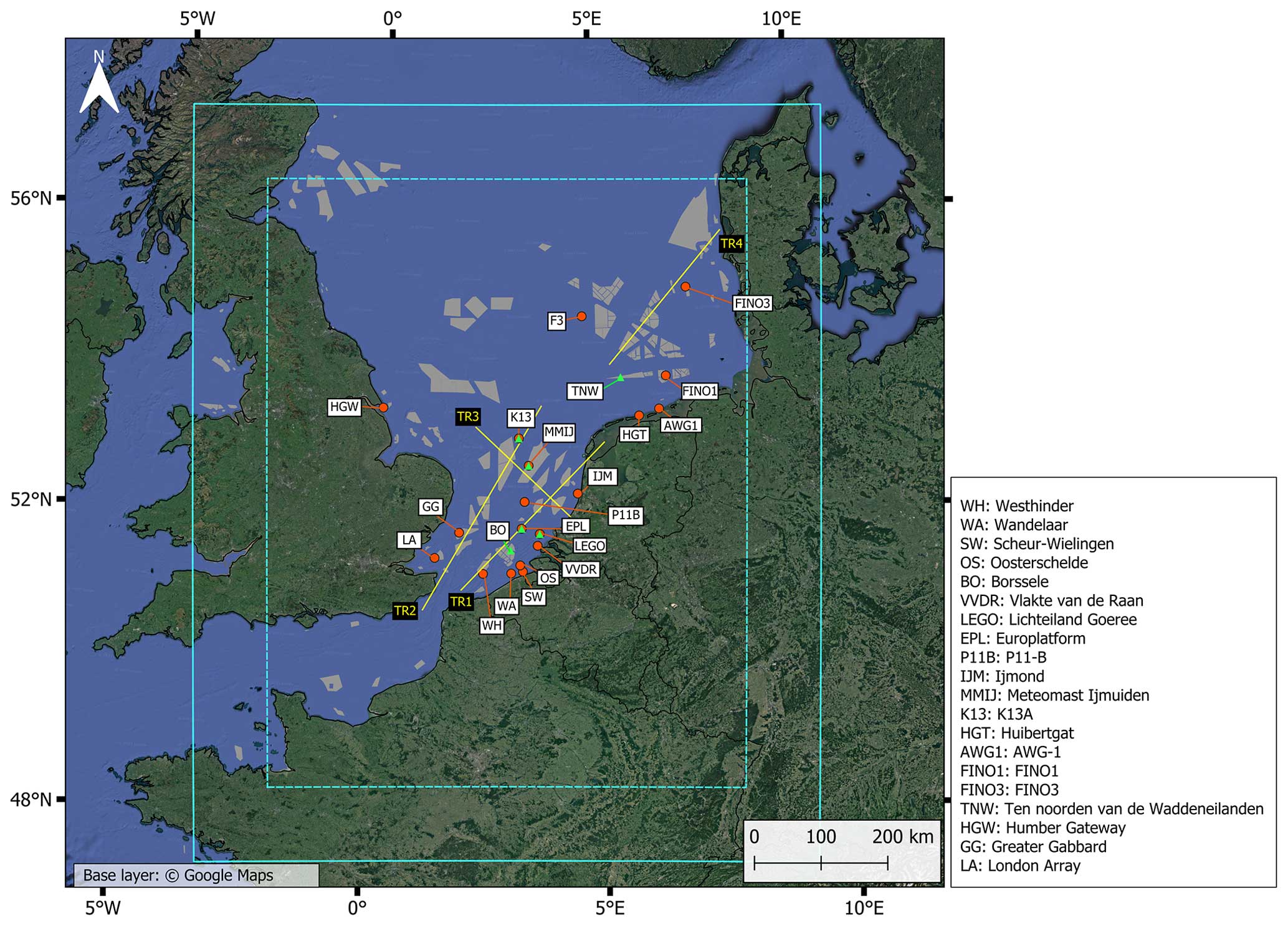
Figure 1 Map of the study area showing the simulation domain (cyan, solid line) and the evaluation domain (cyan, dashed line). The locations of the in situ measurement stations (orange dots) and lidar stations (green triangles) that are used for the model evaluation are also indicated, in addition to the hypothetical future wind farm layout (grey polygons) and the four analysis transects TR1–TR4 (yellow lines) used for the wind farm simulations. Created using QGIS3.4.

The simulation domain covered a large fraction of the North Sea with a horizontal grid spacing of 0.025° (∼2.8 km) (Fig. 1). In the vertical dimension, 61 levels were used up to an elevation of 22 km with a spacing of approximately 20 m near the surface and 30 m at turbine hub height. The relaxation zone at the lateral boundaries was set to a width of 40 km, whereas the spin-up zone was considered an additional 73 km wide, in agreement with the recommendations of Matte et al. (2017). The remaining inner part of the simulation domain was considered for the evaluation and analysis (Fig. 1). The ERA5 reanalysis (Hersbach et al., 2020) was used as forcing at the boundaries with updates every hour. No additional nesting stages were used, in line with results from Brisson et al. (2015). At the meso-γ scale, the model resolution partly allows the explicit development of deep convection so that only shallow convection was parametrized according to the scheme of Tiedtke (1989). Switching of the deep convection parametrization on this resolution has previously been shown not to degrade COSMO simulations (Vergara-Temprado et al., 2020). In COSMO5.0, the TKE advection term in the prognostic equation is only included for the experimental, LES-type turbulence schemes. With the focus on wind farm wake development in the second part of this study, we implemented the TKE advection term for the standard turbulence scheme in COSMO5.0 based on version 5.01.

Specific to this study, we also employed the Fitch wind farm parametrization (WFP; Fitch et al., 2012), which has been implemented in COSMO5-CLM15 (Chatterjee et al., 2016; Akhtar and Chatterjee, 2020). This additional module represents the wind farm forcing on the atmosphere as a sink of kinetic energy and a source of TKE. Although it has been suggested to reduce the TKE coefficient in the parametrization based on a comparison with large eddy simulations (LES) (Archer et al., 2020), the original value was retained in this study, as other studies did not find that this leads to better performance (Siedersleben et al., 2020; Larsén and Fischereit, 2021). Several other wind farm parametrizations exist (Fischereit et al., 2022a), and it has been shown that the modelled wind speed deficits inside and behind a wind farm can vary substantially from the Fitch WFP (Ali et al., 2023). However, validation of the Fitch WFP with offshore masts, lidars and airborne measurements in the wake of a wind farm has shown very good performance for HARMONIE-AROME as wind speed biases are strongly reduced (van Stratum et al., 2022; Dirksen et al., 2022). This good performance has also been determined in WRF by comparing to offshore masts (Garcia-Santiago et al., 2022) and in COSMO-CLM by comparing to LES (Chatterjee et al., 2016) and airborne measurements (Akhtar et al., 2021). Wind speed reductions inside of a wind farm have also been shown to agree well with airborne measurements (Ali et al., 2023), mast measurements (Dirksen et al., 2022) and RANS simulations (Fischereit et al., 2022c). Moreover, comparisons with other WFP schemes show that Fitch generally outperforms these other schemes, both inside a wind farm and in the farm wake (Fischereit et al., 2022c; Ali et al., 2023). For a detailed overview of the performance validation of this parametrization, we refer to the review of Fischereit et al. (2022a).

2.2 Evaluation run

To evaluate the model performance, a simulation was performed for a period of 13 years (2008–2020). Data from in situ, lidar and satellite measurements over the North Sea are abundant in both space and time for this period. Additionally, the length of the simulation ensures that a large variation in wind conditions, as described in e.g. Geyer et al. (2015) and Ronda et al. (2017), is sampled. The wind farm parametrization was excluded in this simulation because a time-static wind farm layout cannot represent the rapidly growing wind farm layout over this time period and most observations were representative for wind-farm-free conditions. Hence, only the undisturbed wind climate was evaluated, and the observations were filtered accordingly, which will be discussed in more detail in Sect. 2.4.1. The instantaneous wind field around hub height was written to output at a 10 min frequency following the standard for wind energy assessments (Menezes et al., 2020).

2.3 Wind farm simulations

The projected future wind farm layout used in the wind farm simulations was constructed from the EMODnet wind farm dataset (EMODnet, 2022) and GIS data from the Royal Belgian Institute for Natural Sciences (Vigin, 2022) (Fig. 1). Next to the operational wind farms today, this layout incorporates the concessions that are in different stages of the construction process, zones for which consent has been authorized and also large development zones. Because the wind farm parametrization assumes that turbines within a single grid cell never have any wake interactions, no additional information is required on the layout of the turbines in each wind farm. The turbines were assumed constantly operational, unless the wind speed was below the cut-in wind speed or above the cut-out wind speed. Considering the computational cost of these experiments, the time span was limited to one representative year in terms of the North Sea wind field. This year was determined in a procedure based on the one outlined in Tammelin et al. (2013). We used 31 years of hourly, hub-height wind fields from the ERA5 reanalysis (1990–2020) to compute a metric R for the representativeness per year and per grid cell:

$$\begin{array}{}\text{(1)}& R_{i,j,y}={\displaystyle \frac{\mathrm{S}{\mathrm{1}}_{i,j,y}}{{\mathit{\sigma }}_{\mathrm{S}\mathrm{1}}}}+{\displaystyle \frac{\mathrm{S}{\mathrm{2}}_{i,j,y}}{{\mathit{\sigma }}_{\mathrm{S}\mathrm{2}}}}+{\displaystyle \frac{\mathrm{S}{\mathrm{3}}_{i,j,y}}{{\mathit{\sigma }}_{\mathrm{S}\mathrm{3}}}},\end{array}$$

where the indices i, j and y refers to a specific grid cell and year. These R values were computed per year for each North Sea grid cell between 51 and 55.5° latitude. Higher values of R correspond to more representative years. The different scores (S1–S3) are based on the agreement between single-year and the long-term (31 year) histograms as computed by the Perkins skill score:

$$\begin{array}{}\text{(2)}& \mathrm{PSS}\left(H_{\mathrm{1}},H_{\mathrm{2}}\right)=\sum _{b=\mathrm{1}}^n\mathrm{MIN}\left(F_{H_{\mathrm{1}}}^{\mathrm{b}},F_{H_{\mathrm{2}}}^{\mathrm{b}}\right),\end{array}$$

where H₁ and H₂ represent the first and second histogram and F^b represents the normalized frequency for bin b. The PSS represents the fraction of overlap between the two histograms, so that a PSS of 1 (or 100 %) represents complete overlap. For one-dimensional histograms, this metric is connected to the Earth mover's distance (EMD) metric, which in contrast represents the area of mismatch between two histograms (Rabin et al., 2008). S1 is the PSS between a wind speed histogram for a single-year and the multi-year wind speed histogram, using a bin width of 0.5 m s⁻¹. S2 is the same as S1 but for wind direction, using a bin width of 30°. Finally, S3 represents the mean PSS between the single- and multi-year wind speed distributions over 12 wind direction sectors. The scores (S1–S3) are standardized by the standard deviation to give each term in the sum equal weight. Summation of R over all grid cells then yields a representativeness for a specific year. The different scores and the final score per year are summarized in Figs. S1 and S2 in the Supplement, respectively. Based on this procedure, the year 2016 was selected for the simulations, as the representativeness is high overall for this year (Fig. S1). In addition, the representativeness is especially high for wind direction (Fig. S2), which is particularly important for the study of inter-farm wake interactions.

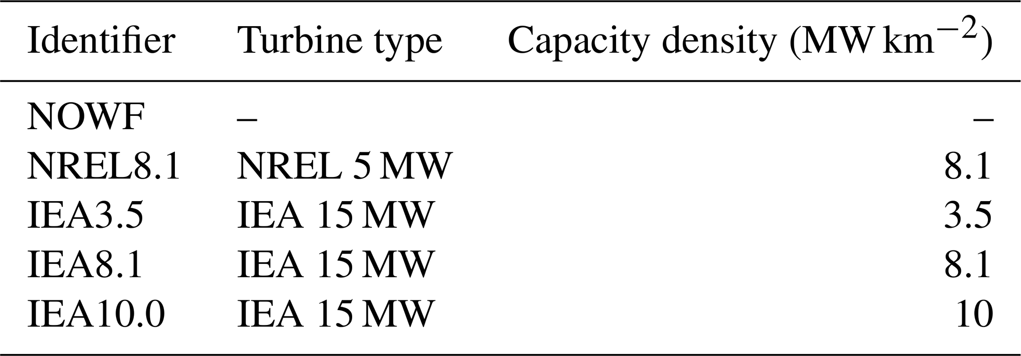
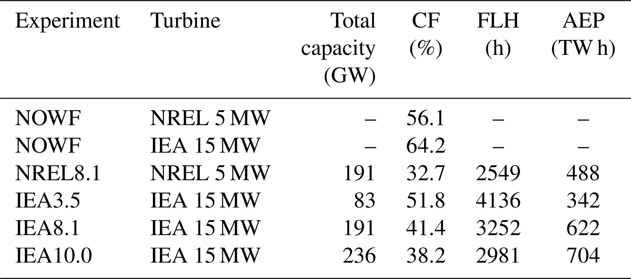
Five simulations were performed, consisting of one simulation without wind farms (NOWF) and four simulations using a fixed wind farm layout with the same turbine type and capacity density for all wind farms (Table 1). Based on the number of turbines, the total capacity and the surface area of operational wind farms in the North Sea, a median turbine capacity of 4.85 MW and a representative capacity density of 8.1 MW km⁻² were determined. The 5 MW reference wind turbine of the National Renewable Energy Laboratory (NREL) (Jonkman et al., 2009)) with a hub height of 90 m and a rotor diameter of 126 m was therefore used in conjunction with the aforementioned capacity density in one of the wind farm simulations (NREL8.1). Three additional cases were simulated in which the NREL 5 MW was replaced by the 15 MW reference wind turbine of the International Energy Agency (IEA) (Gaertner et al., 2020) with a hub height of 150 m and a rotor diameter of 240 m, as 15 MW turbines are expected to reach the market in a few years and are now being selected for upcoming projects (Bento and Fontes, 2019; Shields et al., 2021). The power curves of these three turbines are available in Fig. S3. The three cases with 15 MW turbines were simulated with a different wind farm capacity density.

• IEA3.5: low capacity density in which the inter-turbine distance is 10 rotor diameters. This turbine spacing is larger than is found in most offshore wind farms today and corresponds to a lower cost per unit energy production as the impact of turbine wakes is reduced and is most relevant in regions where offshore space is relatively abundant, such as for the United Kingdom or Denmark (Borrmann et al., 2018).

• IEA8.1: the same capacity density as for the NREL8.1 scenario.

• IEA10.0: high capacity density with a larger revenue per unit area but also increased wake-related losses. This corresponds to a capacity density for planned projects in regions where the available space is limited, such as Belgium, the Netherlands and Germany (Borrmann et al., 2018).

Table 1 Summary of the turbine type and capacity density used in the different wind farm model simulations.

Based on the different simulations, the impact of the turbine type and capacity density on the wake losses was assessed. In addition, the roles of wind farm size and inter-farm distance in these wake losses were investigated based on the large variation in these properties over the wind farm layout. The different simulations were compared along the transects indicated on Fig. 1, which correspond to dominant but also strongly disturbed wind directions, i.e. directions along which the wind farms are densely clustered. For this analysis, only winds in a sector of 30° around the transect orientation (SW to NE for TR1, TR2 and TR4 and NW to SE for TR3) were selected based on the centre grid cell on the transect. The data selection based on the wind direction reduced the dataset to approximately 14 % of the total for transects TR1, TR2 and TR4 and to 8.1 % for TR3. Additionally, this transect analysis was extended to three stability classes based on the bulk Richardson number (R_B), a metric for the dynamic stability, which will be discussed in more detail in Sect. 2.5.3.

2.4 Measurement data

2.4.1 In situ masts

Wind measurements of 19 in situ stations (Fig. 1) were obtained from the KNMI data platform, Meetnet Vlaamse Banken, the Marine Data Exchange, the FINO data platform and the TNO wind energy data platform (Table A1). Of these 19 stations, 6 were actual meteorological masts with measuring devices at multiple altitudes. The remaining stations correspond to coastal measurement poles and instrumentation mounted on oil, gas or light platforms and provide information at a single altitude. Average wind speed and wind direction are available at 10 min intervals. A timeline of the data availability is summarized for each station in Fig. S4. For most stations, corrections were applied to the measurements of the boom- or platform-mounted anemometers and wind vanes in order to account for flow distortions by the mast or other mounting infrastructure. These corrections were performed by the data providers for the stations FINO1 and FINO3 (Westerhellweg et al., 2012; Leiding et al., 2016), MMIJ (Werkhoven and Verhoef, 2012), WH and WA. For the remaining stations with multiple anemometers per height level, we avoided using measurements in the wake of the mast or other infrastructure by selecting the measurement with the highest 10 min average wind speed. A possible drawback of this approach is that the measured wind speed is overestimated in the case of lateral speed-up effects (Leiding et al., 2016). If wind direction was provided with respect to magnetic north, a magnetic-to-true north correction was applied according to the location and timing of the dataset. Finally, because no wind farm parametrization was included in the evaluation run, measurements potentially taken in the wake of wind farms were omitted from the dataset by filtering out either a specific time range or a directional sector. These dataset corrections are summarized in Table S1 in the Supplement. A station-to-farm distance threshold of 50 km was chosen to perform these corrections, as it is expected that the impact of wind farm wakes on the long-term wind speed statistics becomes relatively unimportant at this distance (Schneemann et al., 2020; Dirksen et al., 2022). The total uncertainty on the wind speed measurements is a combination of the uncertainties of calibration, mounting (including flow obstruction by the mast), data acquisition and the local site conditions. This total uncertainty can vary significantly between the stations. For the class 0.9A anemometers at station MMIJ the total uncertainty was estimated at 1.5 % for the top anemometer and 1.9 % for the boom-mounted anemometers (Duncan et al., 2019). For the top anemometers of the other meteorological masts, which have a comparable class number as for MMIJ (Friis Pedersen et al., 2006), we applied the same value of 1.5 % as the uncertainty estimate. As the boom-mounted anemometers at the FINO stations were also mast-corrected prior to use, we adopted the same value of 1.9 %. The mounting uncertainty for boom anemometers at stations GG, LA and HGW is expected to be larger because we only performed a simple correction. Assuming an additional 2 % uncertainty on the mast correction, this leads to a total uncertainty of 3.7 %. For the remaining stations, we assumed a calibration uncertainty of 1.5% (Coquilla et al., 2007), an operational uncertainty of 0.8 % (Friis Pedersen et al., 2006) and an augmented 2 % uncertainty on the data acquisition due to limited information on acquisition and post-processing. For AWG1, P11B and WH a mounting uncertainty of 5 % was estimated due to presence of lateral flow obstructions. For the other stations, where the device is mounted on the top of a platform or platform-mounted mast, a mounting uncertainty of 2 % was assumed following Verkaik (2001).

2.4.2 Wind lidar

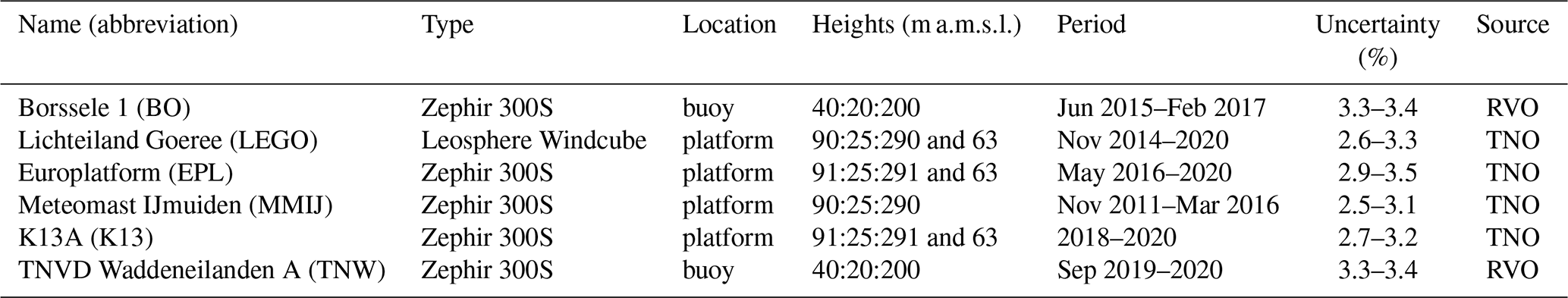
In addition to the cup anemometers, measurements from six wind lidars were used for the evaluation (Fig. 1). These lidars use light beam scanning technology to derive vertical profiles of wind speed and direction at regular height intervals and allow evaluation of the wind field above the typical 90 m top of meteorological masts. As for the in situ measurements, wind speed and direction are provided as 10 min averages. The data were obtained from the Dutch services TNO wind energy and Rijksdienst voor Ondernemend Nederland (RVO). The lidars were installed during the pre-construction stages of offshore wind farm development (Table A2). The LEGO, MMIJ, K13 and EPL lidars are installed on the same platforms as the cup anemometers (Table A1). The BO and TNW lidars are floating lidars and are mounted on a Fugro SEAWATCH buoy. Estimates of the uncertainty are from Wouters and Verhoef (2019a, b, c) for LEGO, EPL and K13; from Poveda and Wouters (2015) for MMIJ; and from the report by Dhirendra (2014) for the floating lidars BO and TNW.

2.4.3 ASCAT

The Advanced SCATterometer (ASCAT) sensor on the European MetOp satellites uses radar technology to determine the near-surface wind speed and direction over the sea (Gelsthorpe et al., 2000; Figa-Saldaña et al., 2002). Although the ASCAT product only provides information on the surface wind, it complements the in situ and lidar data as it covers most of the North Sea basin. For this study, we considered the L3-reprocessed ascending and descending passes of the MetOp-A satellite from the website of the Copernicus Marine Service (CMEMS). The satellite was operational for the complete 13 years of this simulation. Specifically, the variant on a 12.5 km grid with a horizontal grid spacing of 25 km was used, which has been validated against buoy measurements (Verhoef and Stoffelen, 2009). The long-term instrumental stability is estimated to be below 0.1 m s⁻¹ for this product, whereas the climatological uncertainty is ±0.1 m s⁻¹, with some anomalies of +1 m s⁻¹ at the Dutch coast. The datasets for both passes together provide roughly one instantaneous measurement per day for most of the North Sea that we consider (4500 samples in total). Only close to the coasts is data coverage much lower (100–3000 samples), which is a well-known issue with remotely sensed winds related to contamination with land signal (Bourassa et al., 2019).

2.5 Evaluation approach

2.5.1 Model collocation with in situ and lidar

Over a 10 min period, the wind travels over a distance comparable to the edge length of a 0.025° grid cell. Because the model wind components represent smoothed grid box averages, the 10 min time averages of the observations were directly compared to instantaneous values of the grid cell in which the station is located. In the case of gaps in the time series of the in situ and lidar data, the corresponding time steps were also eliminated from the model grid point time series. The model wind speed data were interpolated to the measurement heights using the wind profile power law:

$$\begin{array}{}\text{(3)}& V_{\mathrm{s}}=V\left(h_{\mathrm{m}}\right)\cdot {\left({\displaystyle \frac{h_{\mathrm{s}}}{h_m}}\right)}^{\mathit{\alpha }},\end{array}$$

where V_s is the wind speed at sensor height, V(h_m) is the wind speed at the first model level below sensor height and α is the shear coefficient which is computed as

$$\begin{array}{}\text{(4)}& \mathit{\alpha }={\displaystyle \frac{\ln \left(V\left(h_{m+\mathrm{1}}\right)/V\left(h_m\right)\right)}{\ln \left(h_{m+\mathrm{1}}/h_m\right)}},\end{array}$$

where m+1 denotes the first model level above sensor height. In contrast to the wind speed, the model wind direction at sensor height was computed after linear interpolation of the horizontal wind components of the model levels just above and below sensor height. The Zephir 300S lidar has a well-known 180° ambiguity that can occur in the wind direction time series as it relies on a sonic anemometer just above the lidar to determine the sign of the wind vector. In the case of low wind speeds and/or flow obstructions, it is possible that the incorrect sign is determined and the lidar's wind direction is 180° off (Knoop et al., 2021). We corrected this 180° error by adding or subtracting 180° if the wind direction in the measurements differs more than 90° from the modelled wind direction (∼2 % occurrence) after Dirksen et al. (2022).

2.5.2 Model collocation with ASCAT and triple collocation

For the comparison with ASCAT, the model surface winds were regridded to the 12.5 km grid of the measurements with first-order conservative remapping. This ensures that all the source grid cells contained within a target grid cell have similar weight in the regridding, in agreement with the ASCAT winds being computed from the signal of this complete area. Afterwards, the measurement time series of each ASCAT grid cell was matched by a model time series for that same grid cell by linear interpolation in time.

Additionally, a comparison between the model, ASCAT and in situ data was conducted at stations WH, EPL and MMIJ. These stations were selected because the location is far enough from the coast to ensure sufficient data points in the ASCAT data and the measurement height is close to 10 m, which reduces any vertical extrapolation errors to 10 m in the in situ data. This extrapolation was done using the power law with a constant shear coefficient of 0.11. The in situ data were then also linearly interpolated to the ASCAT measurement times, and all datasets were limited to the timings where both ASCAT and in situ measurements are available. Finally, the grid cells in which the stations are located were selected from the model and ASCAT datasets for the comparison.

2.5.3 Stability classification

The comparison between COSMO-CLM and the measurements in terms of wind speed was further extended to different classes of atmospheric, dynamic stability because the stability strongly determines the wind conditions over the North Sea (Stull, 1988; Sathe et al., 2011) and also determines the atmospheric response to a wind farm forcing (Platis et al., 2021). This stability classification was done based on the bulk Richardson number (R_B), which is computed as

$$\begin{array}{}\text{(5)}& R_{\mathrm{B}}={\displaystyle \frac{\frac{g}{\stackrel{\mathrm{‾}}{{\mathit{\theta }}_{\mathrm{v}}}}\frac{\mathrm{\Delta }{\mathit{\theta }}_{\mathrm{v}}}{\mathrm{\Delta }z}}{{\left(\frac{\mathrm{\Delta }u}{\mathrm{\Delta }z}\right)}^{\mathrm{2}}+{\left(\frac{\mathrm{\Delta }v}{\mathrm{\Delta }z}\right)}^{\mathrm{2}}}},\end{array}$$

where g corresponds to the gravitational constant, θ_v is the virtual potential temperature, z is height, and u and v are the zonal and meridional wind speed components, respectively. The overbar over the virtual potential temperature denotes that it is averaged over the four model layers between 50 and 150 m height. Finally, the gradients in u, v and θ_v were determined by averaging the gradients between each of the subsequent layers between 50 and 150 m. Based on the (R_B), we can identify three distinct dynamic stability regimes (Grachev et al., 2013; Dirksen et al., 2022).

• Unstable: R_B<0. This is the case when the temperature gradient is negative, which corresponds to an unstable thermal stratification.

• Weakly stable: $\mathrm{0}\le R_{\mathrm{B}}\le \mathrm{0.25}$. This is the case when the temperature gradient is positive, but the temperature effect is weak compared to the vertical wind shear. In this case, the wind-shear-generated turbulence is relatively strong compared to the buoyant damping.

• Stable: R_B>0.25. This is the case when the temperature gradient is positive and strong compared to the vertical shear. In this case, the wind-shear-generated turbulence is strongly damped, and this region of the ABL can be considered dynamically stable.

Gradients were calculated based on potential temperature instead of virtual potential temperature as an analysis of the driving data showed minimal variations of specific humidity over the considered height range. A comparison of the modelled temperature gradients with measured temperature gradients at station MMIJ between 90 and 21 m a.m.s.l. shows a good correspondence in the long-term temperature gradient probability distribution, indicating sufficient model skill for this subdivision into stability classes (Fig. S5). Because vertical profiles of pressure and temperature are generally not available over the range of the meteorological masts or wind lidar scanning ranges, the stability criterion can only be computed for the model. Based on a good temporal correlation between the temperature gradients of COSMO-CLM and measurement mast MMIJ (Pearson correlation coefficient = 0.85), the time steps matched to a stability class for the model grid cell nearest to each measurement location were also matched to that stability class for the measurement data.

2.5.4 Evaluation metrics

We compared the magnitudes of the mean wind speed difference and the observational uncertainty to identify any model bias: an exceedance of the observational uncertainty at a measurement station was used as the threshold for the presence of a model bias at that location. In addition, the PSS (Sect. 2.3) was employed as a metric to express the agreement in the shape of two histograms of either wind speed or wind direction.

Because the relationship between wind speed and wind turbine power production is non-linear, we also evaluated differences between COSMO-CLM and the observations in terms of the capacity factor, which is given by

$$\begin{array}{}\text{(6)}& \mathrm{CF}=\mathrm{100}{\displaystyle \frac{\sum _{i=\mathrm{1}}^{n}P\left(V_i\right)}{nP\left(V_{\mathrm{r}}\right)}}\left[\mathit{\%}\right],\end{array}$$

where V_i is the hub-height wind speed at some instance i in the time series; V_r is the rated wind speed; and P is the generated power, which is a turbine-specific function of the wind speed. So, the capacity factor is the ratio between the power production of a specific turbine based on a wind speed time series and the theoretical, maximum power production over that same period, i.e. for a turbine continuously operating at full capacity. This is an idealized notion of the capacity factor as it concerns an isolated turbine which constantly operates according to the power curve. For these calculations, we considered the power curve of the NREL 5 MW reference wind turbine, with a hub height of 90 m, for the meteorological masts with the top anemometer below 100 m and the power curve of the DTU 10 MW reference wind turbine (Bak et al., 2013), with a hub height of 119 m, for FINO1, FINO3 and the wind lidars (Fig. S3). An uncertainty range on the capacity factor based on the observed wind speeds was determined based on the uncertainty on the wind speed measurements: the observed wind speed distribution was shifted linearly by the product of the uncertainty and the mean wind speed after which upper and lower bounds on the capacity factor were computed. As the capacity factor is a percentage, absolute differences are also a percentage, so to avoid confusion it is always explicitly stated whether absolute or relative differences in the capacity factor are considered.

3 Results and discussion

3.1 Model evaluation

This subsection covers the model performance evaluation. First, the general evaluation based on all validation sources and the complete height range (10 to 290 m) is described. This is followed by a more detailed performance analysis at turbine hub height (∼100 m), and finally the evaluation is extended to the different atmospheric stability classes.

The difference in the long-term mean wind speed between the in situ and lidar stations varies with height (Fig. 2). Below 90 m, the difference is generally negative (model underestimates the mean) and exceeds the measurement uncertainty range, indicating a model bias to lower wind speeds. However, the magnitude of the bias generally drops with increasing altitude over the considered height range, albeit with some exceptions (MMIJ, TNW). At measurement heights at or above 90 m, the difference is generally smaller and falls within the uncertainty range of the measurements. The gradient with height persists and the difference is positive above 130 m at the locations of the wind lidars. Although differences over height are substantial, there is no robust indication of regional differences in the ability of COSMO-CLM to model the climatological mean wind speed. The same figure but with relative differences is included in the Supplement (Fig. S6).

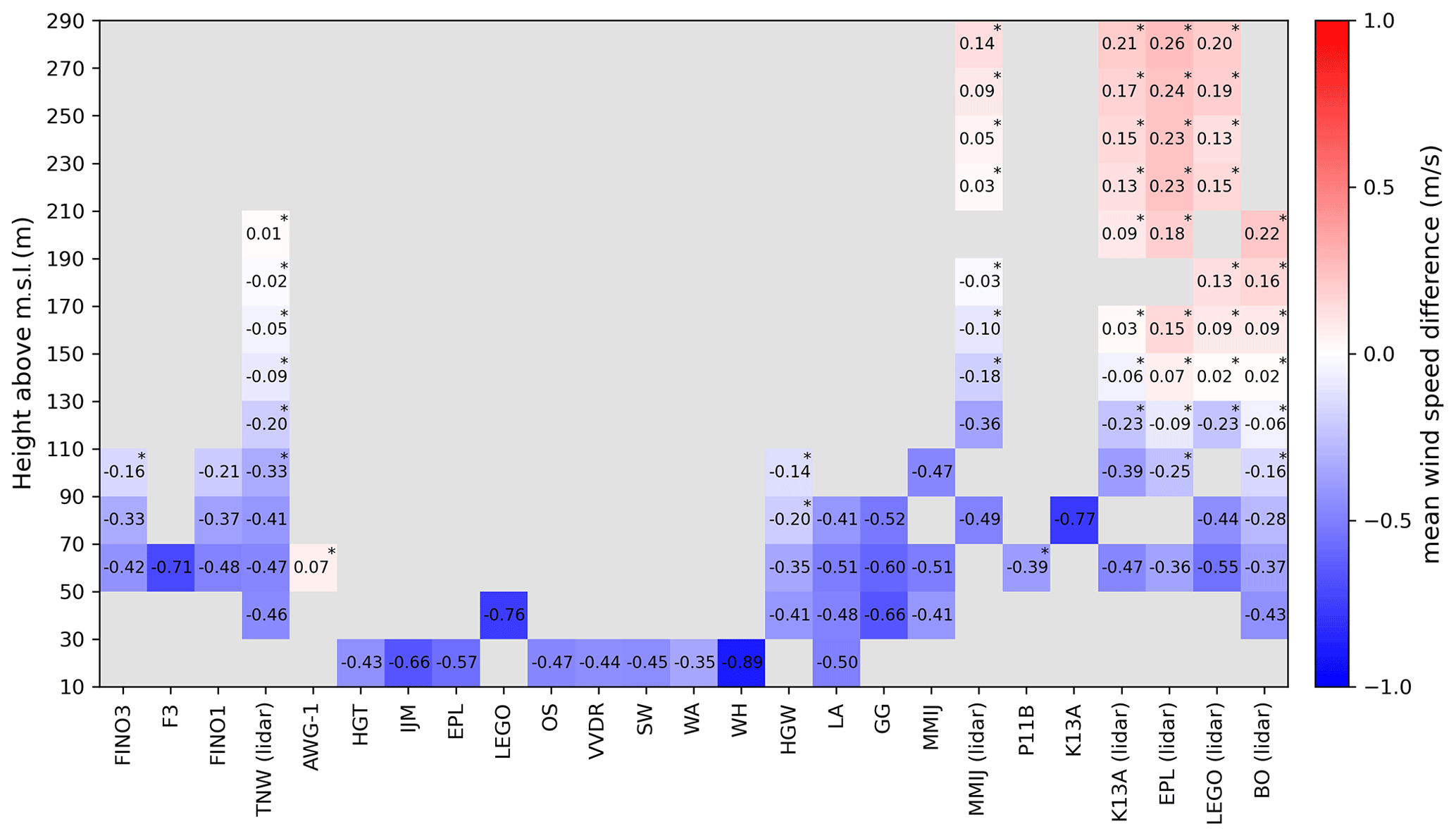
Figure 2 Wind speed bias (m s⁻¹) for the complete time span of each measurement dataset. This concerns measurements between 10 and 290 m a.m.s.l. The vertical range is subdivided into 20 m intervals for readability. The presence of an asterisk indicates that the bias is within the measurement uncertainty. Stations are clustered per region. The considered time periods for each measurement dataset can be found in Tables A1 and A2.

The mean difference between COSMO-CLM and the ASCAT data is between −0.5 and 0.5 m s⁻¹ for most grid cells (Fig. 3). For approximately 45 % of the grid cells the mean difference is within the ASCAT climatological uncertainty of ±0.1 m s⁻¹. These grid cells are generally located farther from the coast and correspond to the regions without in situ measurements, which is an indication of good model performance in this region. The model underestimation near the surface that was identified against the in situ data in the southern North Sea is much smaller than the differences compared to ASCAT in this region (cf. Figs. 2 and 3). A three-way comparison with three in situ stations shows that the mean differences against the in situ data exceed the in situ measurement uncertainty for both COSMO-CLM and ASCAT (Fig. 3). Whereas COSMO-CLM generally underestimates the mean near-surface wind speed, ASCAT overestimates it with a larger magnitude, which explains the differences in PSS values. The PSS values are similar when both COSMO-CLM and ASCAT are corrected for the systematic bias with respect to the in situ data, which indicates that both perform similarly in approximating the distribution shape of the in situ data.

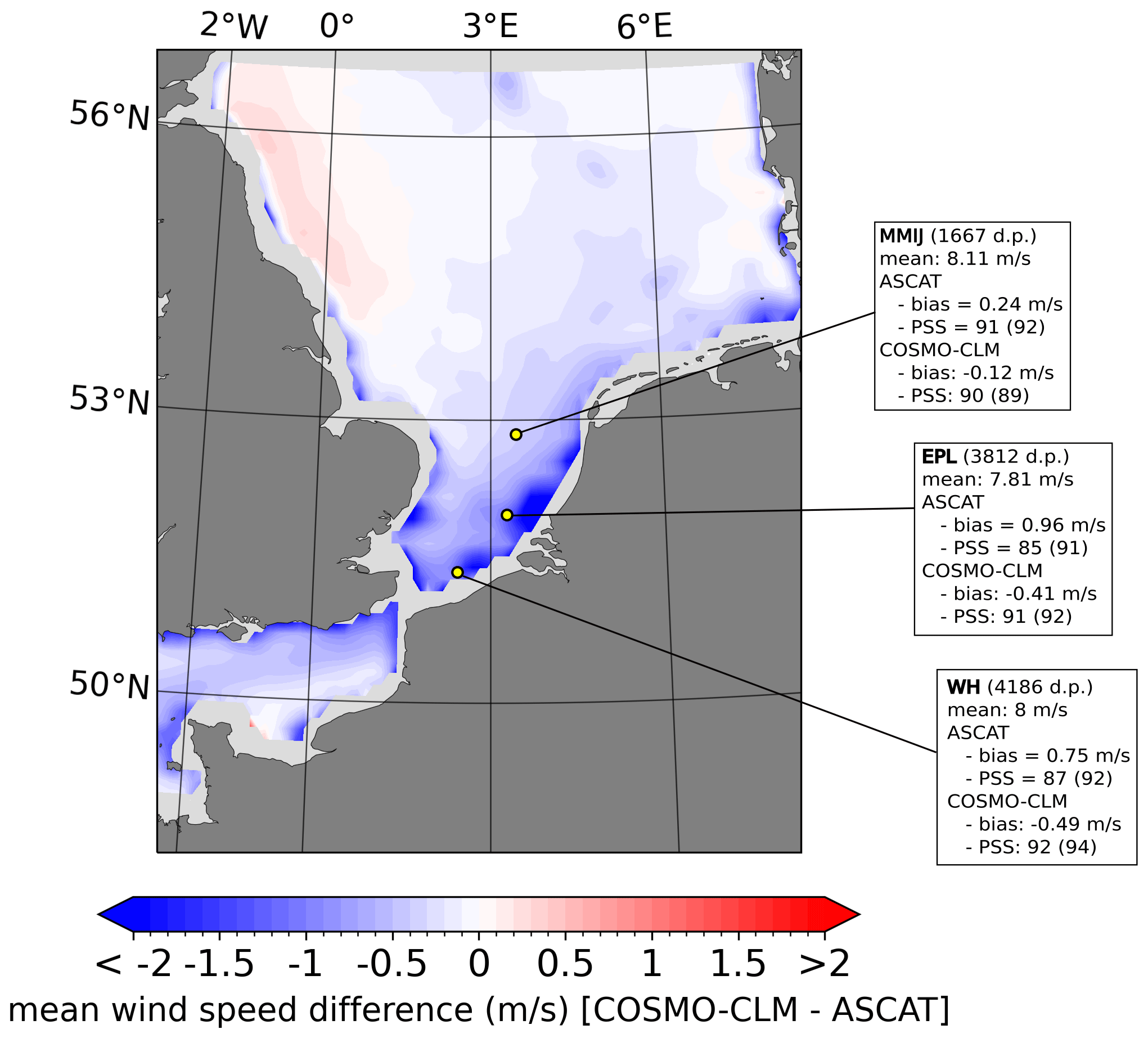
Figure 3 Difference in long-term mean wind speed between COSMO-CLM and ASCAT. Yellow dots indicate the measurement stations for triple collocation. The text boxes summarize the mean 10 m wind speed for three in situ stations and the agreement of ASCAT and COSMO-CLM in terms of the mean difference and the PSS. The PSS values between brackets are after elimination of the mean difference between the two histograms to remove the effect of distribution location.

The distributions of wind speed near 100 m height match well with the meteorological masts and lidar stations in most cases (Fig. 4), leading to a PSS generally above 95 %. The associated absolute differences in the idealized capacity factor are within the uncertainty based on the wind speed measurements for 4 out of 10 stations. For FINO1, K13, MMIJ and HGW the differences are outside the uncertainty range, but the deviations from the lower bound of the uncertainty range are less than 1 %, while the deviations are higher for the GG and LA masts. For K13 and HGW the capacity factor difference exceeds the capacity factor uncertainty, whereas the mean wind speed difference is within the wind speed uncertainty, which can be linked to the non-linear relationship between wind speed and power production.

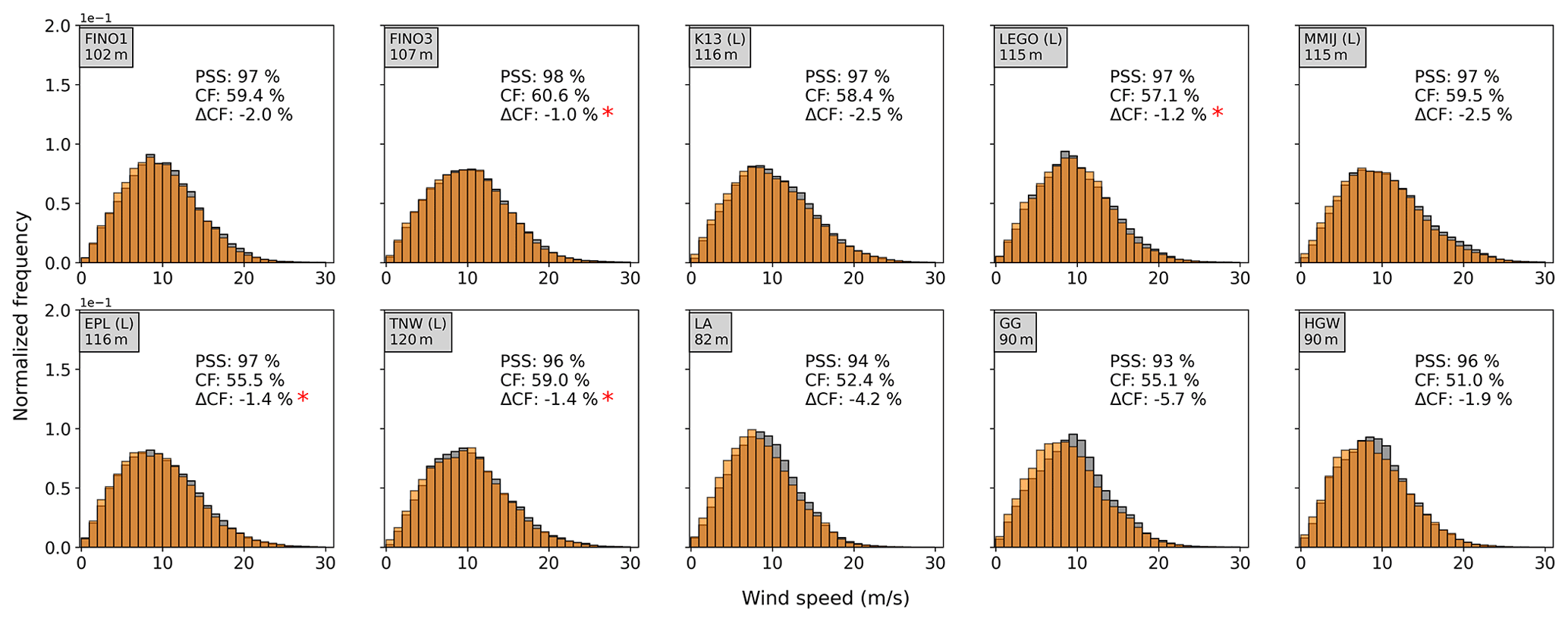
Figure 4 Histograms of the collocated wind speed datasets. Orange: overlap between the histograms; light orange: only COSMO-CLM; grey: only the measurements. In addition, the associated PSS, the capacity factor based on the measured wind speeds and the absolute difference in capacity factor between the model and the measurements are indicated. The presence of a red asterisk indicates that the capacity factor difference falls within the uncertainty on the capacity factor for the measurements.

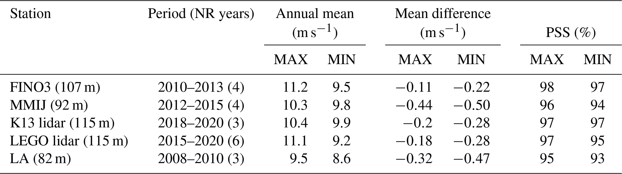
Although the inter-annual variability of the annual mean hub-height wind speed is typically around 1 m s⁻¹, the corresponding variability in the wind speed bias between the model and the measurements is typically around 0.1 m s⁻¹ or 10 % of that value (Table 2). The corresponding overlap between the single-year histograms generally does not vary more than 2 % over the years. Hence, the agreement in distribution location and shape between COSMO-CLM and the measurements remains consistent over consecutive years, regardless of the inter-annual variability in the wind conditions.

Table 2 Inter-annual range of the mean wind speed and of the agreement between the model and observations, as expressed by the minimum/maximum annual mean difference and the minimum/maximum annual PSS for the different years in the measurement period.

The intra-annual cycle in the wind speed distribution is also well represented by the model (Fig. 5). The gradual seasonal variation from higher (winter) to lower (summer) median wind speeds is accurately reproduced in addition to the variation in distribution width (Q₂₅–Q₇₅ range) and more extreme conditions (Q₅ and Q₉₅). Moreover, in extreme months the model also succeeds in modelling the wind speed distribution as can be deduced from Fig. 5b at station TNW for February 2020, albeit with a heavier right tail and consequently more winds above the cut-out wind speed.

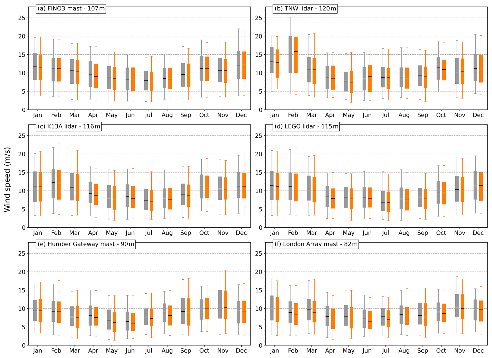
Figure 5 Boxplots representing the multi-year wind speed distribution per month for the observations (grey) and the model (orange). Shown for the three masts and three lidar stations at turbine hub height. The box corresponds to the Q₂₅–Q₅₀–Q₇₅ wind speeds. The lower and upper whiskers are the Q₅ and the Q₉₅ percentiles, respectively.

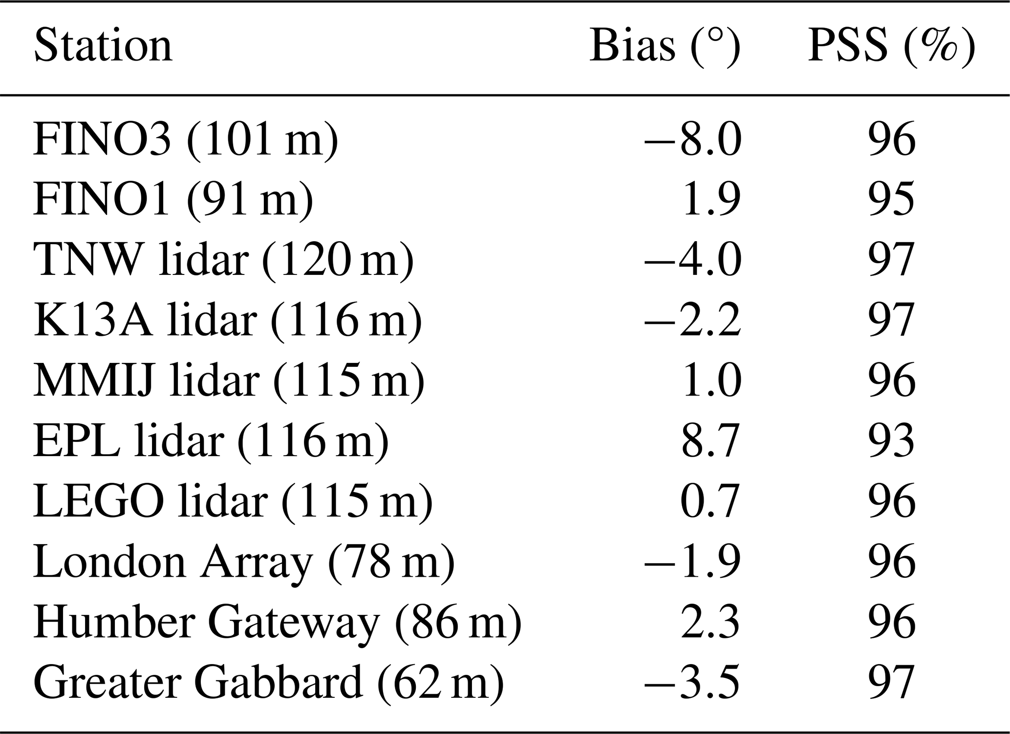
Evaluation of the long-term wind direction histograms near turbine hub height (using a bin width of 20°) shows an overlap of 95 % or more in most cases (Table 3) with the magnitude of the bias generally below 4°. A reason for the stronger deviation at FINO3 and EPL has not been identified. Because the considered measurements vary substantially in measurement height, i.e. from 62 m a.m.s.l. up to 120 m a.m.s.l., this comparison indicates consistency of the good performance with height. The variations of the wind speed statistics with the wind direction are also captured by the model (Fig. S7). This accurate reproduction of the wind direction distributions and the direction-dependent wind speed distributions is encouraging for the application to wind farm modelling as wind farm shapes are tailored to the regional wind climate.

Table 3 Bias in the wind direction (model – observations) and the Perkins skill score between the histograms of wind direction (bin width = 20°).

The general differences in mean wind speed profiles for the three stability classes agree well between the model and the measurements (Fig. 6): winds are strongest under weakly stable conditions and weakest under stable conditions, with the wind speeds under unstable conditions falling in between. The agreement between the profiles of the model and the measurements differs between the stability classes: under stable conditions the shear in the model is too strong between 40 and 200 m, leading to a negative model bias below 160 m for EPL and LEGO and below 180 m for K13 and TNW. Around 100 m, the respective underestimations are at least −0.3 and −0.6 m s⁻¹. Such an underestimation under stable conditions is not uncommon for climate models (Wijnant et al., 2014; Sheridan et al., 2021). For weakly stable conditions, there is not a clear bias around 100 m, but the deviations below 90 m and above 150 m are outside of the observational uncertainty. The small vertical gradient under unstable conditions is represented well by the model with only small deviations that are well within the measurement uncertainty over the complete height range. The hub-height wind speed distributions as reflected in the boxplot mainly differ in distribution location, with the strongest differences under stable conditions. Corresponding capacity factor values were calculated with lower and upper uncertainty bounds for the observations (Fig. S8). Under stable conditions, the deviations between the model and observations exceed the uncertainty range, so the absolute model underestimation of the capacity factor is at least 2.5 %. For unstable and weakly stable conditions, the deviations are within the uncertainty range.

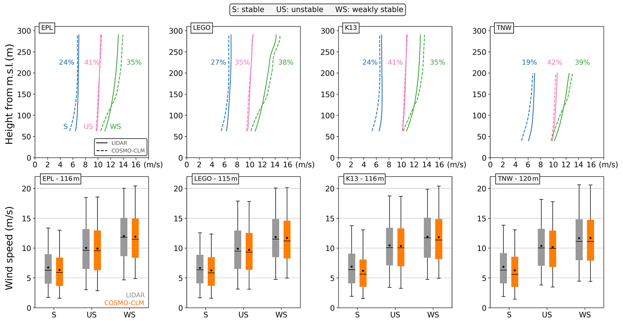
Figure 6 Model evaluation for different stability classes. Top row: vertical profiles of the mean wind speed per stability class for four lidar stations (full line) and the corresponding model output (dashed line). The stability classes are stable (blue), unstable (pink) and weakly stable (green). The indicated percentages are the relative frequency of the different stability classes at hub height. Bottom row: boxplots of the hub-height wind speeds per stability class for the same four lidar stations (grey) and the corresponding model output (orange). The box corresponds to the Q₂₅–Q₅₀–Q₇₅ wind speeds. The asterisk indicates the mean, and the lower and upper whiskers are the Q₅ and the Q₉₅ percentiles, respectively.

3.2 Impact of wind farm characteristics on cluster-scale wake losses

This subsection covers the results of the wind farm simulations. First, the impact of the NREL8.1 base scenario on the wind climate and wind resource is described, also under different atmospheric stability conditions. Afterwards, the different wind farm scenarios are compared in terms of cluster-scale wake effects and efficiency of power production.

The modelled mean wind speed at 90 m for 2016 varies from 7.5 m s⁻¹ at the coast up to 10 m s⁻¹ in the open North Sea (Fig. 7). The associated capacity factor varies between 45 % and 60 %, and the simulated pattern agrees well with earlier, multi-decadal estimates over the North Sea (Geyer et al., 2015). Stability separation shows that the capacity factors are generally largest under weakly stable conditions and can reach 75 % in the open North Sea. For stable conditions, capacity factors are considerably lower but also prone to the bias discussed in Sect. 3.1. The bottom row of Fig. 7 visualizes the impact of the projected, future wind farm layout if they were all occupied with NREL 5 MW turbines at 8.1 MW km⁻². Without subdividing for stability, the absolute reductions of the full-year capacity factor in the immediate vicinity of farms located in dense clusters are around 15 %, with cumulative contributions from multiple wind farms. The magnitude of the long-term resource reductions is similar to what other studies have identified in terms of closely spaced wind farms (Akhtar et al., 2021; Fischereit et al., 2022b). Very close to the larger farms, larger values can be found even when the farms are isolated. The absolute and relative changes in the capacity factor vary over the stability classes. Absolute capacity factor reductions are typically the smallest for stable conditions, but these are the largest in relative terms as capacity factors are small themselves. In weakly stable conditions, absolute capacity factor reductions are much higher, as these exceed 13 % over large zones within and outside the wind farm clusters and 5 % more than 20 km from wind farm clusters and larger wind farms.

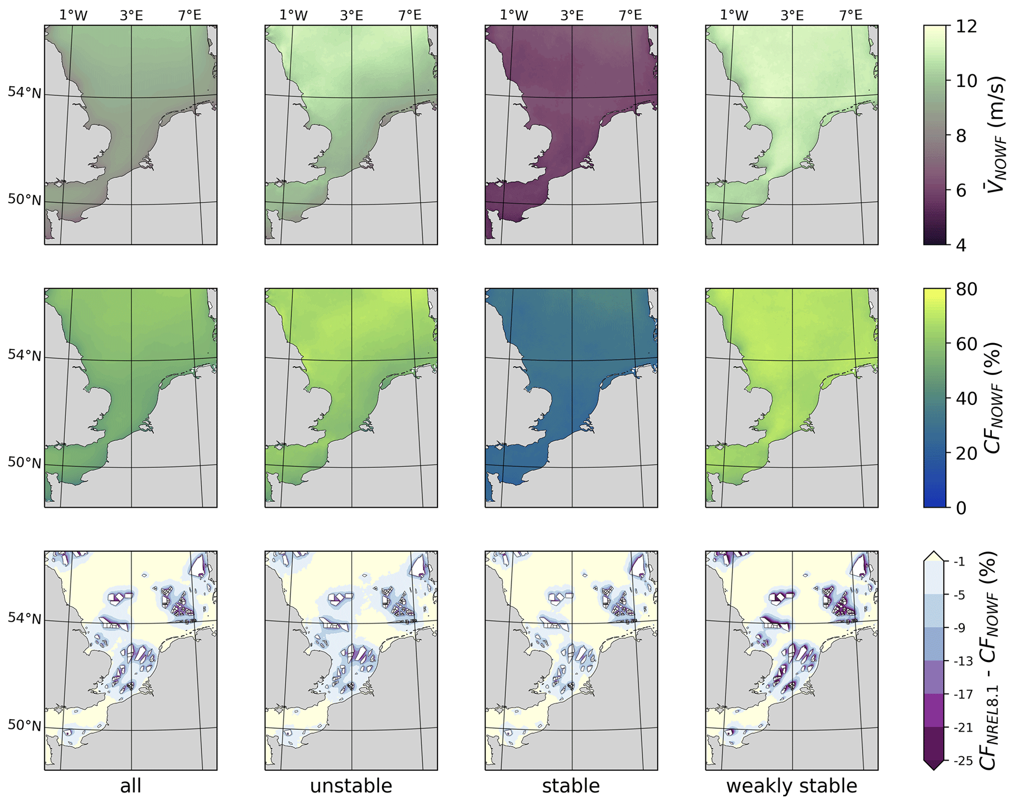
Figure 7 Maps of the modelled North Sea wind climatology at 90 m a.m.s.l., the corresponding wind resource in terms of the capacity factor, and the resource deficit under the NREL8.1 scenario for the complete year and for the three stability classes. Top: maps of the yearly mean wind speed (m s⁻¹) under the NOWF scenario. Middle: capacity factor under the NOWF scenario (%). Bottom: absolute capacity factor deficit for the NREL8.1 scenario (%). White polygons represent wind farm locations. Capacity factor computations are based on the power curve of the NREL 5 MW wind turbine.

The impact of the atmospheric stability on the wind-farm-induced reduction in hub-height wind speed can be analysed in more detail along the four analysis transects (Fig. 8). For TR1, TR2 and TR4, the data are dominated by weakly stable conditions (∼65 %) compared to unstable (∼19 %) and stable (∼16 %) conditions, whereas for TR3 unstable conditions are more prevalent (∼59 %) compared to stable (∼29 %) and weakly stable (∼12 %) conditions. The relative reductions at the end of wind farms typically exceed 20 % for all stability classes, but reductions are generally smaller for unstable conditions than for stable and weakly stable conditions. However, the transects do not show a significantly slower wind farm wake recovery for stable conditions, as has been found based on observations (Cañadillas et al., 2020; Platis et al., 2021). The presented transect analysis also differs strongly from such studies in that it considers time averages of different wind speeds and covers a very large extent with the stability and wind direction criterion only evaluated at the centre of the transects. Added to that, modifications of dynamic stability by wind farms, which has previously been modelled with LES (Porté-Agel et al., 2014; Lu and Porté-Agel, 2015), could be strongly enhanced by the large, non-existent wind farms used in this study. The associated capacity factor profiles show that the relative impact on the wind resource is large for all stability classes (Fig. S9). The forcing by large wind farms and clusters can lead to a halving of the capacity factor for all stability classes in some transect sections. The relative impact on the capacity factor values is much larger than for the mean wind speed, due to the non-linearity of the turbine power curves (Fig. S3).

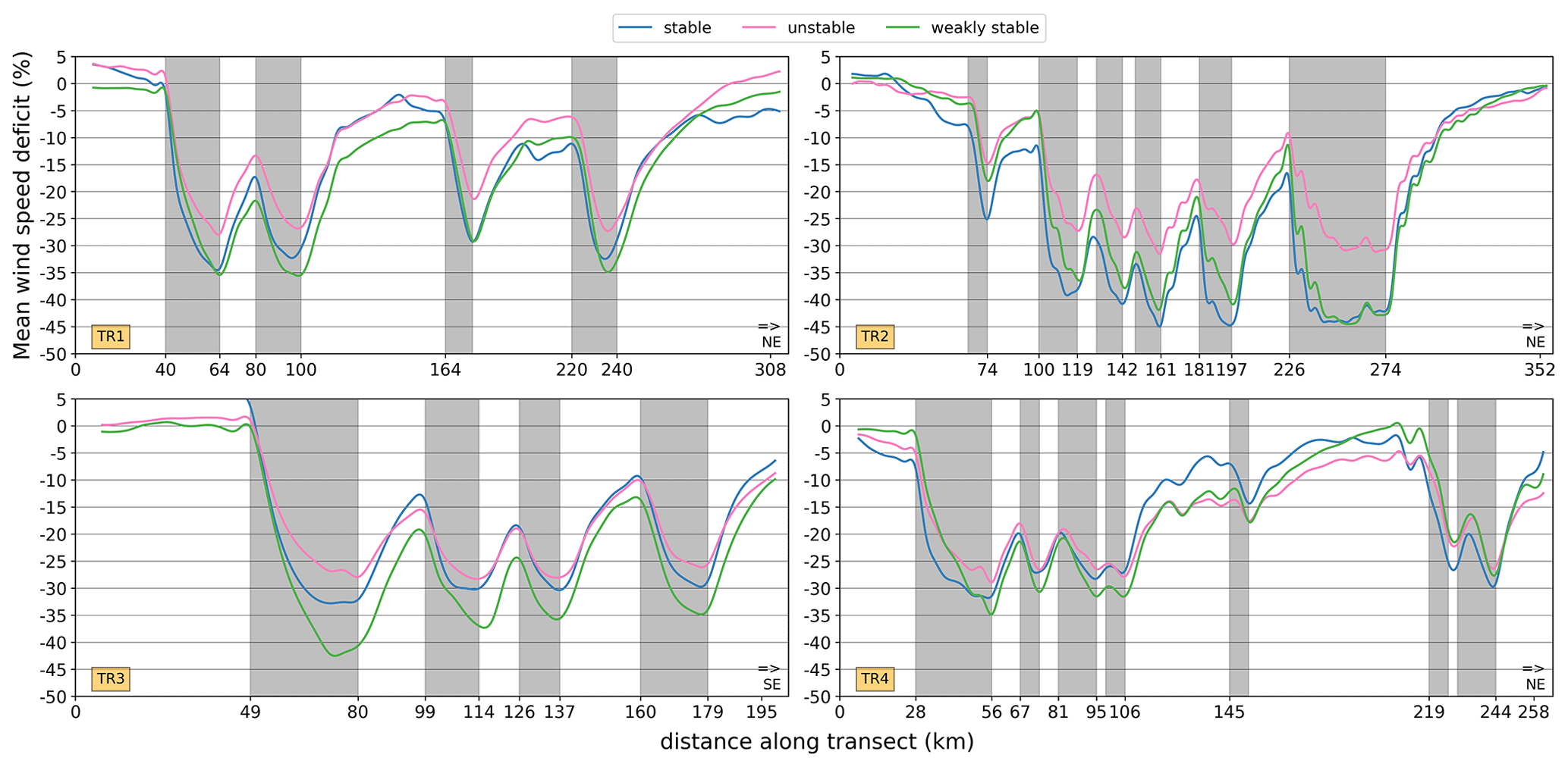
Figure 8 Relative deficit of the along-transect mean wind speed (%) at 90 m a.m.s.l. for the four transects indicated on Fig. 1. This concerns the NREL8.1 scenario, subdivided in the three dynamic stability classes: unstable (pink), weakly stable (green) and stable (blue) according to the R_B. Wind data are only considered when the wind direction deviates within ±15° from the transect orientation (W to E) at the middle grid cell of each transect. Grey shadings represent wind farm locations.

The wind farm capacity density used in the different wind farm simulations strongly determines the mean wind speed profile along these transects (Fig. 9). In each case, zones of densely clustered farms (<20 km apart) are characterized by the strongest reductions and a limited farm wake recovery that is typically less than half of the maximum deficit at the previous wind farm. The scenario with IEA 15 MW turbines at 3.5 MW km⁻² is characterized by the smallest reductions, which are typically within 1.5 m s⁻¹ at the upwind side of wind farms. For higher capacity densities, these upwind edge reductions are often more than twice as large and can exceed 3 m s⁻¹ under very dense clustering. Only for recovery distances of 30–60 km, the IEA8.1 and IEA10.0 scenarios converge to within 0.5 m s⁻¹ of the IEA3.5 scenario. Furthermore, the impact of wind farm size on the intensity of the reduction can be assessed by focusing on the first wind farm in each transect: the larger wind farms of TR1, TR3 and TR4 have an along-transect farm length between 24 and 31 km, while this is only 9 km for the one in TR2. The associated reductions at the downwind edge of the wind farms are approximately twice as large for TR1, TR3 and TR4 than for TR2.

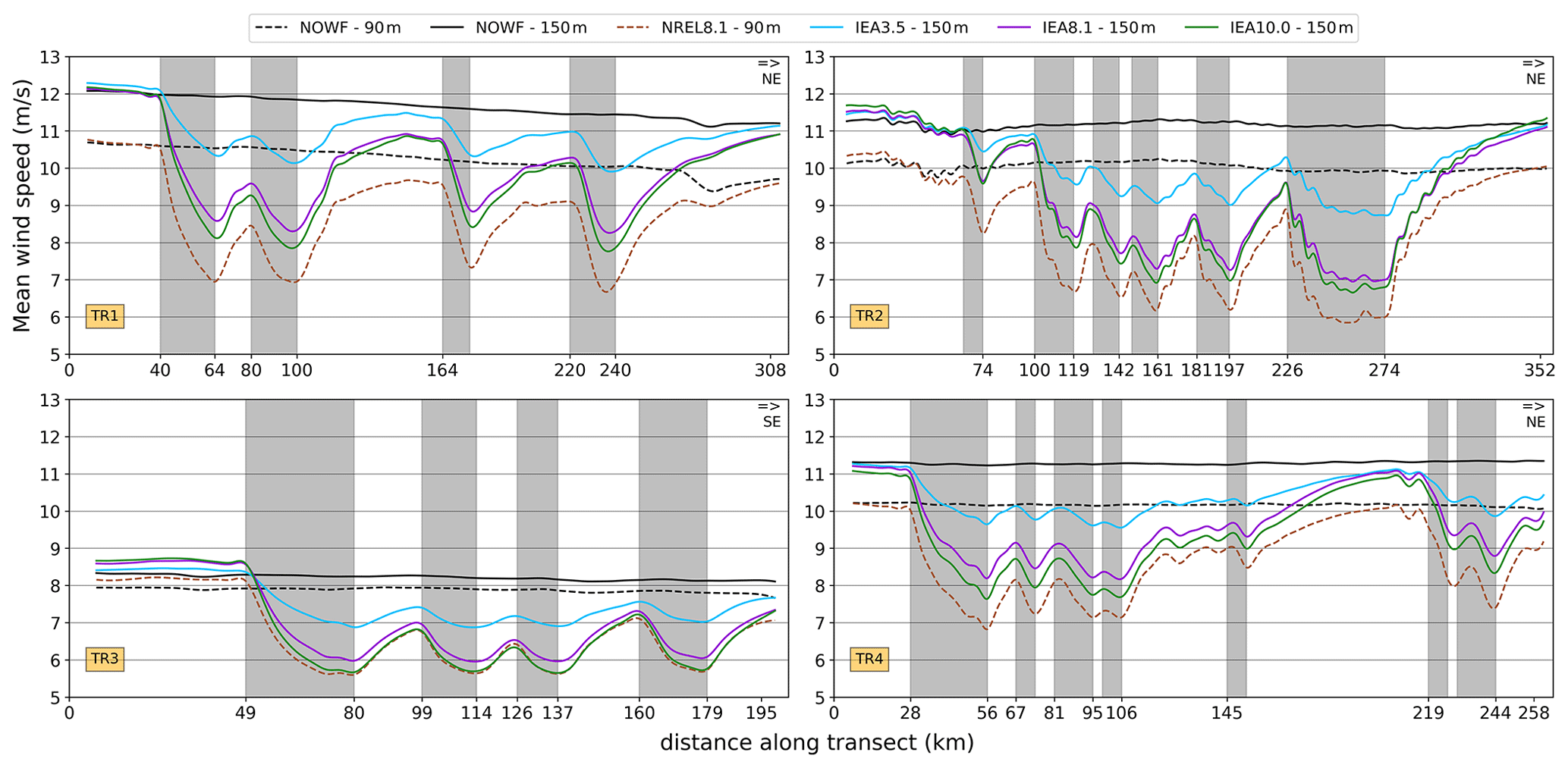
Figure 9 Transects of the mean wind speed at turbine hub height for the different wind farm scenarios. These transects correspond to the four lines in Fig. 1. Wind data are only considered when the wind direction deviates within ±15° from the transect orientation (W to E) at the middle grid cell of each transect. Grey shadings represent wind farm locations.

When converting the wind speed information of the NOWF scenario into capacity factors, the transect averages are ∼58 % for TR1, TR2 and TR4 and ∼38 % for TR3 when considering the hub height and power curve of the NREL 5 MW turbine. For the IEA 15 MW turbine, these increase to ∼66 % and ∼46%, respectively. Figure 10 shows that the associated, absolute reductions in these capacity factor follow the general patterns established for the mean wind speed. In each transect, the IEA3.5 scenario is characterized by the smallest deficits at the upwind edge of wind farms, typically around 10 % with larger values in dense clusters. For higher capacity densities, the upwind edge reductions reach 25 % to 30 % for closely spaced wind farms. The intensity of these upwind edge reductions is strongly dependent on the degree of upwind clustering and the sizes of the upwind farms. For the scenarios with higher capacity densities, the superposition of the high momentum sink on the already intense farm wake deficit eventually results in much lower wind farm efficiencies for these scenarios. For the SW–NE-oriented transects, the impact of the turbine type becomes apparent: for the 90 m turbines in the NREL8.1 scenario, the absolute deficits over the wind farms exceed those of the IEA8.1 scenario, which translates to a much stronger reduction in relative terms as the unaltered (NOWF) capacity factors for the 5 MW turbines are lower than for the 15 MW turbines.

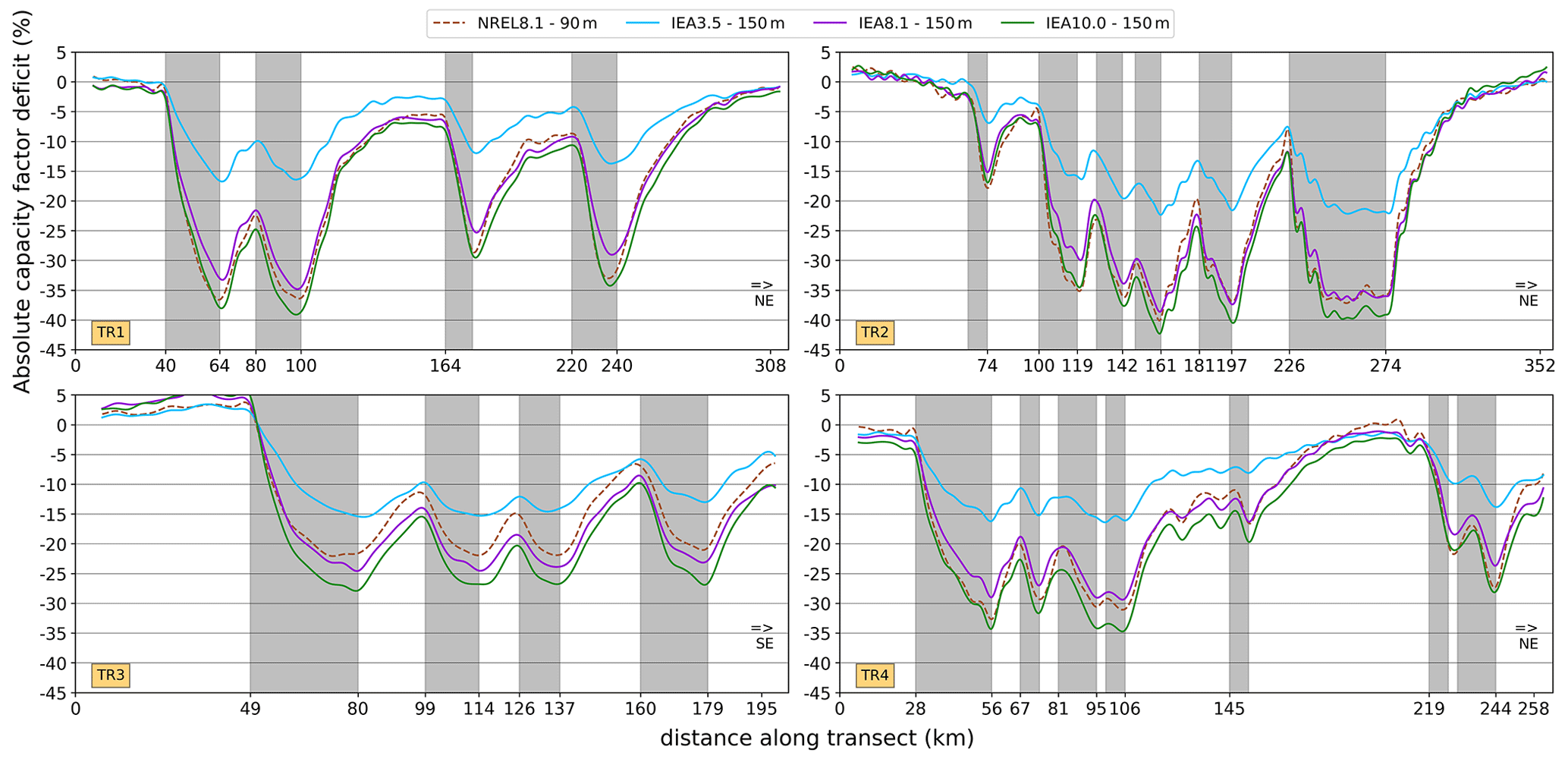
Figure 10 Transects of the absolute capacity factor deficit at hub height for the different wind farm scenarios. These transects correspond to the four lines in Fig. 1. Wind data are only considered when the wind direction deviates within ±15° from the transect orientation (W to E) at the middle grid cell of each transect. Grey shadings represent wind farm locations.

The wind farm layout in the IEA8.1 scenario is significantly more efficient than for the NREL8.1 scenario, as reflected in the layout-integrated capacity factor and full load hours in the evaluation domain (Table 4). As a consequence, the integrated AEP is 27.4 % higher in the former. This difference is partly due to the rated wind speed being 0.8 m s⁻¹ lower for the 15 MW turbines so that the rated section of the power curve is more wide (Fig. S2). Added to that, taller turbines can take advantage of the wind speed gradient with height, which leads to a larger fraction of wind speeds in the rated regime and a reduced fraction in the steep part of the power curve. To disentangle both effects, the 90 m wind speed data of the NREL8.1 scenario were fed to the 15 MW power curve, which resulted in an AEP of 539 TW h. This implies that approximately 40 % of the increase in AEP can be attributed to the lower rated wind speed and approximately 60 % to the wind speed gradient with height. Combining 15 MW turbines with a low capacity density of 3.5 MW km⁻² only reduces the integrated capacity factor from 64.2 % in the NOWF scenario to 51.8 %, as a consequence of limited intra- and inter-farm wake impacts, in agreement with Meyers and Meneveau (2012) and Gupta and Baidya Roy (2021). From IEA3.5 to IEA8.1, the capacity density increases by 131 %, whereas the AEP only increases by 82 %. From IEA8.1 to IEA10.0, these increases are 23.4 % and 13.1 %, respectively. This efficiency degradation when moving to larger capacity densities can be recognized in a reduced capacity factor and a reduction in the full load hours (FLH): compared to IEA3.5, the IEA10.0 capacity factor is reduced from 51.8 % to 38.2 % and the FLH is reduced by approximately 1150 h. This follows from the increased wake losses that are further exacerbated by the densely clustered layout and the presence of several large wind farms that are typically characterized by very low power densities (Volker et al., 2017).

Table 4 Annual energy and power metrics integrated over all wind farms in the evaluation domain. CF: layout-integrated capacity factor. FLH: full load hours for the complete layout. AEP: annual energy production for the complete layout. The calculations are based on the wind speed data of the wind farm grid cells. The capacity factors for the NOWF simulation correspond to efficiency in absence of intra- and inter-farm wakes.

4 Conclusions

We have used the regional climate model COSMO-CLM to quantify the dependence of long-term, cluster-scale wake losses on the turbine type, capacity density, wind farm spacing and wind farm size for a hypothetical future wind farm layout. First, the model skill in simulating the wind climate was evaluated in a comparison with in situ, lidar and satellite data, which revealed the following.

• The differences between the measured and modelled, long-term mean wind speed at turbine hub height (∼100 m) are generally within the measurement uncertainty. This is also the case for differences at higher altitudes (up to 290 m), but closer to the surface COSMO-CLM underestimates the mean wind speed ($\sim -\mathrm{0.5}$ m s⁻¹). Under stable stratification (∼25 %), the model underestimates the long-term mean wind speed at turbine height but not under weakly stable and unstable stratification (∼75 %).

• The agreement between the measured and modelled, long-term wind speed histograms is high, with a PSS above 95 % in most cases. The theoretical capacity factors derived from these histograms agree well overall, but small underestimations (∼1 %–5 %) are present at some locations.

• The agreement with the wind speed measurements is consistent over the different years of the simulation period as inter-annual variations in the mean wind speed difference and the PSS are small. The seasonal variability in the shape and location of the wind speed distribution is also captured by COSMO-CLM.

• Multi-year histograms of wind direction also agree well, with again a PSS above 95 % in most cases. The variation of the wind speed histograms over 12 directional bins (30°) is also adequately captured in the model. This encourages the application of COSMO-CLM to wind farm modelling as wind farm shapes are adapted to the regional wind climate.

As deviations mainly occur under stable conditions, a stability-dependent bias correction could be considered for future applications in addition to continuous efforts to improve the model. Overall, this evaluation emphasizes the value of having a large set of wind measurements available in regions for offshore wind farm development, as it allows a benchmarking of mesoscale models over the region of interest.

The application of the model to a hypothetical, future wind farm layout indicates that the creation of dense wind farm clusters is accompanied by an alteration of the surrounding wind climate and significant farm-to-farm wake interactions. The impact of these interactions depends heavily on the turbine type, the capacity density, the inter-farm spacing and the size of the wind farms. In this study, the comparison of two turbine types (NREL 5 MW and IEA 15 MW) and three capacity densities (3.5, 8.1 and 10 MW km⁻²) show the following.

• For a capacity density of 8.1 MW km⁻², the layout-integrated AEP is ∼27 % larger for a layout of 15 MW turbines than for 5 MW turbines. This difference is linked to the layout-integrated capacity factor being considerably larger when using taller, 15 MW turbines because of the increase in the wind resource with height (60 %) and a lower rated wind speed (40 %). The use of 15 MW turbines compensates for ∼37 % of the wake losses recorded in the NREL8.1 simulation.

• Under dominant wind directions with dense wind farm clustering, the wind resource is strongly reduced due to inter-farm wakes. Assuming 15 MW turbines, the absolute reductions in the capacity factor at the upwind edge of wind farms range from 3 % to 17 % for a capacity density of 3.5 MW km⁻² depending on the degree of clustering and the size of the upwind farms. For a capacity density of 8.1 MW km⁻² this ranges from 5 % to 30 % and for 10 MW km⁻² from 5 % to 33 %.

• Assuming a projected, future wind farm layout with 15 MW turbines, increases in the capacity density of the wind farms lead to strong efficiency reductions. The layout-integrated capacity factor reduces from 51.8 % for a 3.5 MW km⁻² capacity density to 38.2 % for a 10 MW km⁻² capacity density, due to the intensification of intra- and inter-farm wake losses.

• Wind farm wake effects play an important role for all considered atmospheric stability classes, even if the impact is a bit smaller for unstable conditions. Under strongly waked wind directions, the low capacity factors (20 %–30 %) under stable conditions (R_B>0.25) can be further reduced to well below 10 %, thereby nearly completely halting the production of some of the simulated wind farms. Although these results are possibly impacted by the negative model bias that was found for stable stratification, it is expected that this large impact under stable conditions still holds.

Whereas comparisons between wind farm parametrizations have shown large variations in terms of modelled wind speed deficits inside and behind wind farms (Ali et al., 2023), validation efforts in several mesoscale models have indicated a very good performance of the Fitch WFP (Fischereit et al., 2022c; van Stratum et al., 2022; Ali et al., 2023). Nonetheless, the use of other WFP schemes might significantly alter the magnitudes presented here, more so due to the large clusters and large wind farms included in the considered layout, which can even lead to wake losses for background wind speeds well above rated. Hence, further benchmarking studies of WFPs for a range of atmospheric conditions and validation data could help in further reducing this WFP-related uncertainty. An additional complication here is that this study includes wind farms of non-existent sizes for which validations simply do not exist.

Even if the mesoscale wind farm parametrization approach has limitations, these modelling studies provide valuable information for the efficient deployment and operation of offshore wind infrastructure, more so because mesoscale models can consider the climatic variability of wake effects, for large regions. This study demonstrates the potential of this modelling approach to explore a large variety of wind farm characteristics and layouts in a climatic context, which can aid in a more efficient expansion of the offshore infrastructure.

Appendix A

Table A1 Description of the in situ measurement stations. S: wind speed (m ⁻¹); D: wind from direction (°). The superscripts a, b and c link measurement heights to measurement devices in the next column. 1×, 2× and 3× refers to one, two, or three anemometers and/or wind vanes at one measurement height. Source acronyms: KDP, Royal Netherlands Meteorological Institute (KNMI) data platform; MNVB, Meetnet Vlaamse Banken; MDE, the Marine Data Exchange; FINO, Forschungsplattformen in Nord- und Ostsee; TNO, Nederlandse Organisatie voor Toegepast-natuurwetenschappelijk Onderzoek.

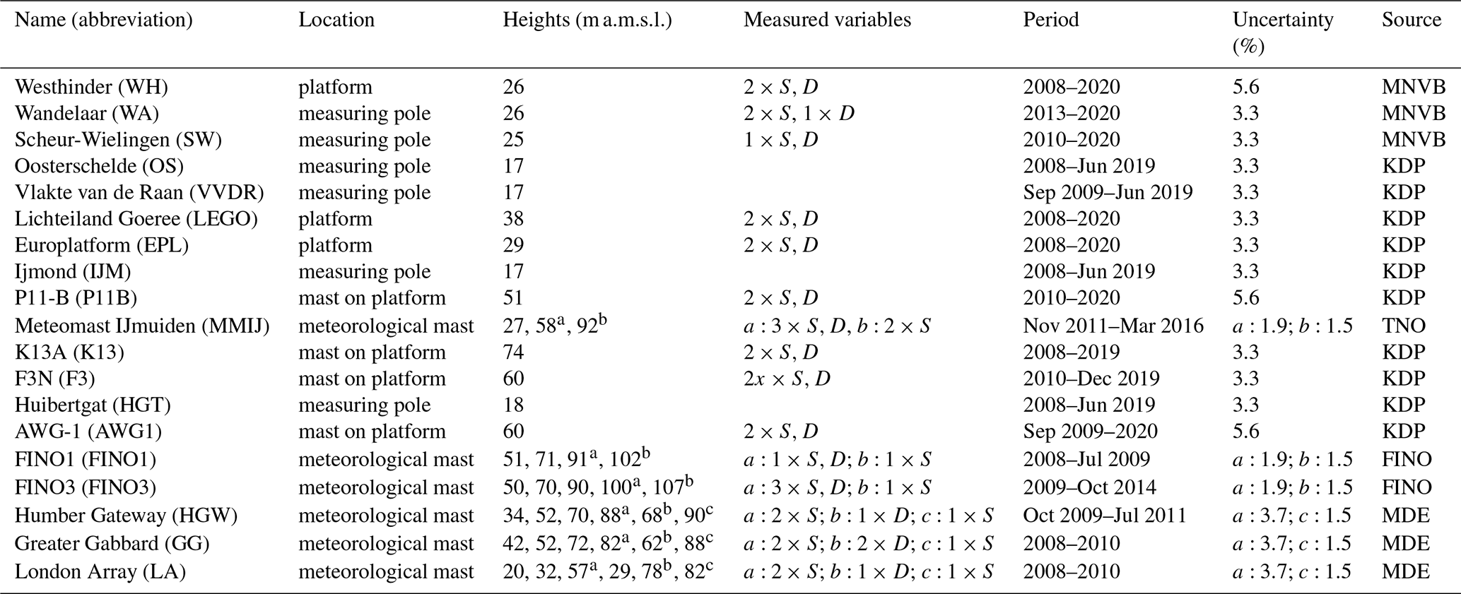
Table A2 Description of the lidar measurement stations. Source acronyms: RVO, Rijksdienst voor Ondernemend Nederland; TNO, Nederlandse Organisatie voor Toegepast-natuurwetenschappelijk Onderzoek.