Review of rolling contact fatigue life calculation for oscillating bearings and application-dependent recommendations for use

In contrast to the multitude of models in the literature for the calculation of rolling contact fatigue in rotating bearings, literature on oscillating bearings is sparse. This work summarizes the available literature on rolling contact fatigue in oscillating bearings. Publications which present various theoretical models are summarized and discussed. A number of errors and misunderstandings are highlighted, information gaps are filled, and common threads between publications are established. Recommendations are given for using the various models for any oscillating bearing in any industrial application. The applicability of these approaches to pitch and yaw bearings of wind turbines is discussed in detail.

1 Introduction

While most bearings in industrial applications rotate, there are some notable ones which are required to oscillate. These include bearings in helicopter rotor blade hinges (Tawresey and Shugarts, 1964; Rumbarger and Jones, 1968), Cardan joints (Breslau and Schlecht, 2020), offshore cranes (Wöll et al., 2018), and blade and yaw bearings in wind turbines, shown in Fig. 1. Blade bearings turn (pitch) the blade around its longitudinal axis to change the blade's angle of attack. Their movements in modern wind turbines mostly consist of small (typically¹ φ<10°, often as small as φ<1°; see Stammler et al., 2020) oscillations with the occasional 90° movement to bring the turbine to a halt. Similarly, yaw bearings rotate the turbine to face into the wind. Their movements are typically fewer and, depending on the site and the yaw system design, longer (<10° during power production but potentially more while idling). Yaw movements do not tend to become as low (φ<1°) as pitch angles (Wenske, 2022).

Rolling contact fatigue is a possible failure mechanism of bearings. It is caused by the fact that, even under a constant external load, movement of the bearing (rotation or oscillation) causes movement of the rolling bodies (balls or rollers) relative to the bearing rings. If the rolling bodies transmit load to the raceway, their movement leads to stress cycles, because every location of the raceway changes from a loaded state while it is in contact with a rolling body to an unloaded one while it is not (see Fig. 6, left-hand side, for a typical case in a rotating bearing). The resulting stress amplitudes can, over time, cause fatigue damage on the raceways or, less frequently, the rolling bodies. The driving stress for rolling contact fatigue is typically considered to be shear stress. Fatigue can be initiated from shear stress below the surface of the raceway (subsurface fatigue) and from shear stress at its surface (surface fatigue) (Lundberg and Palmgren, 1947; Ioannides et al., 1999; Harris and Kotzalas, 2007; Zaretsky, 2013).

Figure 1 Wind turbine pitch bearing (green, also called blade bearing) and yaw bearing (blue). © Fraunhofer IWES, Jens Meier.

Rolling bearings under oscillatory movements are commonly associated with wear damage to the raceways and rolling bodies (Grebe, 2017; Stammler, 2020; Behnke and Schleich, 2023; FVA, 2022b; de La Presilla et al., 2023). Small oscillation amplitudes are generally seen to be a risk factor for wear, particularly in grease-lubricated bearings (Behnke and Schleich, 2023; Stammler, 2020; Grebe, 2017; FVA, 2022b). However, wear can also be prevented by a number of measures (Schwack, 2020; Wandel et al., 2022), and it is definitely possible for rolling contact fatigue to occur without wear² even for oscillating amplitudes as low as θ=1° (φ=2°). Rolling contact fatigue, on the other hand, is always a possible failure mechanism even in a properly designed bearing (Sadeghi et al., 2009), except for very low loads (Ioannides et al., 1999), at which there is dispute about its occurrence (Zaretsky, 2010). In many cases, such as large oscillation amplitudes or the use of oil lubrication, wear is unlikely to occur and, thus, rolling contact fatigue becomes a more important focus. Moreover, depending on its severity, wear in itself does not necessarily cause a complete failure of the bearing, but it can also accelerate rolling contact fatigue (FVA, 2022a, b). Engineers should therefore consider both wear and rolling contact fatigue as possible failure mechanisms. This paper reviews calculation approaches to determining the rolling contact fatigue life of oscillating bearings. There are a number of approaches for rolling contact fatigue life calculation in the literature (see Sadeghi et al., 2009, and Tallian, 1992, for an overview), but they are mostly intended for rotating applications. While any of these could in principle be changed to be used in oscillating applications, this paper collates all approaches that have explicitly been developed for oscillating bearings in general or that are concerned with specific bearings which oscillate, such as pitch bearings.

As part of the introduction, phenomena which are present in oscillating bearings but not in rotating ones are discussed in Sect. 1.1. An overview of calculation approaches is given in Sect. 2. It includes three different commonly used ISO-based factors (Harris, Rumbarger, and Houpert), all of which have been designed for oscillations with a constant amplitude, and a number of other approaches described in the literature. Section 3 gives an overview of experimental results, and Sect. 4 then discusses when to apply these methods, with an example explaining their applicability to pitch and yaw bearings, which oscillate with a varying amplitude.

1.1 Operational conditions of oscillating bearings

Most operating conditions of oscillating bearings are similar to those of rotating bearings, and much has been written about these conditions. Similarities include the load distribution among the rolling elements, which tends to spread as a function of the radial and axial load (Harris and Kotzalas, 2007) and the bending moment, if present. Individual rolling elements experience point or line contacts, originally described by Hertz for balls (Hertz, 1882) and later described by other methods for rollers (Reusner, 1977; de Mul et al., 1986), resulting in contact pressures on the inner and outer ring that tend to be different. The raceways experience cyclic loading, which can cause rolling contact fatigue, often assumed to be caused by shear stress in particular (Lundberg and Palmgren, 1947; Harris and Kotzalas, 2007). In both oscillating and rotating bearings, there can be grease and oil lubrication present (Hamrock et al., 2004), raceway surface quality and lubrication contamination affect the bearing (Ioannides et al., 1999), and so on.

Since this review focuses on oscillating bearings, some differences between rotating and oscillating bearings are, however, worth pointing out. One main difference is simply the travel that a bearing performs when it oscillates as compared to when it rotates: for an oscillation as depicted in Fig. 3, an oscillation arc A is covered. This is typically smaller than the 360° covered during a rotation. Therefore, the life of an oscillating bearing, if measured in oscillations, tends to be bigger than that of an otherwise identical bearing that rotates, measured in revolutions.

One commonly discussed difference is the fact that, for small oscillation angles, only a part of the raceway is ever loaded, while the remaining part is always unloaded. For the bearings depicted in Fig. 4, the bearing on the left side only sees cyclic loading on selected locations of its ring, whereas the bearing on the right side sees loading all over its ring, which is distributed unevenly. In Fig. 2, the blue oscillation pattern (stochastic) causes the entire ring to experience an uneven number of load cycles, depicted in the right of the figure. The red pattern on the other hand only leads to stress cycles in selected locations, exactly like the left part of Fig. 4. All of the aforementioned cases are fundamentally different from a rotating bearing, in which for both the inner and outer ring every location of a ring experiences the same amount of stress cycles if the bearing is rotated for long enough.

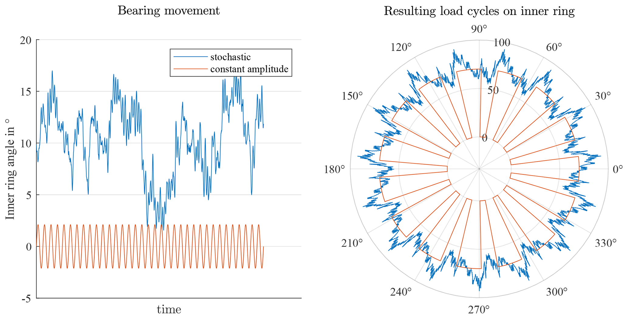
Figure 2 Load cycles resulting from oscillation and stochastic movement in a bearing with Z=15 rolling elements.

Although the stress cycles are evenly distributed on each ring of a rotating bearing, the load is not. It is typically assumed to be constant with respect to one ring, the so-called stationary ring, while the other one rotates relative to it. If the load distribution is uneven, such as the load distribution shown in the top of Fig. 5, this causes the stationary ring to always experience its highest load in the same location. The rotating ring, on the other hand, will have all of its circumferential locations see stress cycles as shown in the bottom of Fig. 5, with only a time shift between the loading of each circumferential location of that rotating ring. For an oscillating bearing, the stationary ring is loaded similarly (identical, if one ignores the fact that there is a discrete amount of rolling elements), but the rotating ring is loaded differently over time: all of its circumferential positions can experience a very different stress cycle history as shown in Fig. 5 for a small and large oscillation amplitude θ.

From a viewpoint of rolling contact fatigue, it is also noteworthy that the stress cycles experienced by the raceway are not identical in an oscillating and a rotating bearing. For a rotating bearing, the left of Fig. 6 shows the typical type of shear stress loading history as assumed in the literature (Lundberg and Palmgren, 1947; Harris and Kotzalas, 2007). The center figure shows that at reversal points of the oscillation, the amplitude of the shear stress can be lower than in a rotating bearing (blue case), and, thereafter, the sign of the shear stress cycle flips (red case). For small oscillations, the right part of Fig. 6 shows that the oscillation amplitude of a rotating bearing may even never be reached.

Aside from these effects that concern the stress cycle history and its distribution over the circumferential locations of the inner and outer ring, lubrication is well known to behave differently in an oscillating bearing as compared to a rotating one, causing a time- and movement-dependent film thickness (Venner and Hagmeijer, 2008). As discussed above, this can cause wear if the lubricant film thickness is bad enough, but even if no wear occurs, a different lubricant film thickness than in a rotating bearing may be present.

2 Existing calculation approaches

There are a number of publications on the issue of rolling contact fatigue in oscillating bearings. Most of them are based on ISO (ISO, 2007, 2008b, a, 2021) or closely related to the model used for ISO. These publications are summarized in Sect. 2.1. Several approaches that have little relation to ISO and its foundations have also been proposed and are discussed in Sect. 2.2. Some of the ISO-related methods are intended for constant oscillation amplitudes as depicted red in Fig. 2, where an oscillation with a constant amplitude about a position of 0° is shown³, while some other ISO-related methods and all non-ISO-related methods are intended for arbitrary movement as depicted in blue in Fig. 2.

2.1 ISO-related approaches

Fundamentally, rolling contact fatigue in oscillating applications is caused by a rolling element repeatedly rolling over locations on a raceway, as is the case in rotating applications. For this reason, many researchers have sought to adapt the well-known ISO approach for rolling contact fatigue calculation to oscillating applications. All of these approaches are hence characterized by the fact that they are based on Lundberg and Palmgren (1947), who proposed that

$$\begin{array}{}\text{(1)}& \ln {\displaystyle \frac{\mathrm{1}}{S}}\propto {\displaystyle \frac{{\mathit{\tau }}_{\mathrm{0}}^c{N}^e}{z_{\mathrm{0}}^h}}V,\end{array}$$

where S is the survival probability, τ₀ is the maximum orthogonal shear stress and z₀ is its depth under the raceway surface at which τ₀ occurs, N is the number of load cycles (rollovers), and V is the loaded volume (Lundberg and Palmgren, 1947, 1952; Harris and Kotzalas, 2007; Zaretsky, 2013).

Lundberg and Palmgren used Eq. (1) to derive their well-known life equation $L_{\mathrm{10},\mathrm{rev}}=(C/P{)}^p$, with dynamic load rating C and dynamic equivalent load P, which remains the basis for ISO 281 (ISO, 2007) and ISO/TS 16281 (ISO, 2008b) as well as countless other publications. They assumed the bearings to be rotating. L_10,rev then gives the number of millions of revolutions at which 10 % of bearings are expected to suffer the first visible raceway damage⁴, also called “basic rating life”. In principle, their derivation can be adapted for use in oscillating movement as well. This section discusses publications which either apply or derive such adaptations of the original Lundberg–Palmgren approach, or approaches very similar to it but also based on Eq. (1). Most of these approaches derive corrective factors a_osc that are intended to be applied to a life measured in revolutions and convert it into a life measured in oscillations, i.e.,

$$\begin{array}{}\text{(2)}& {\displaystyle }{L}_{\mathrm{10},\mathrm{osc}}=a_{\mathrm{osc}}{L}_{\mathrm{10},\mathrm{rev}},\end{array}$$

where L_10,osc is the life measured in oscillations and L_10,rev is the life in revolutions. This equation applies to all so-called “oscillation factors” in this paper. For small oscillation amplitudes, a_osc typically becomes very large, with a_osc commonly (but not always) being in the range of 1 … 1000. All factors a in this paper are instances of a_osc as shown in Eq. (2).

There are two common definitions of an oscillation amplitude; this paper mainly uses θ as defined in Fig. 3. Some equations are also given in terms of the double amplitude φ if there are differences compared to the equation in terms of θ.

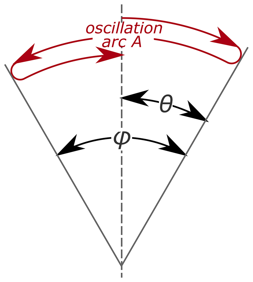
Figure 3 One oscillation covering arc A=4θ (=2φ) with oscillation amplitude θ (and double amplitude φ) as defined in this paper.

2.1.1 Harris: traveled distance

The Harris factor⁵ is given in various editions of Rolling Bearing Analysis by Harris (Harris, 2001; Harris and Kotzalas, 2007). It considers the effect whereby an oscillating bearing will, depending on the oscillation amplitude, experience a different number of stress cycles on the rings than a rotating bearing. The factor can be interpreted as a conversion of traveled distance into an equivalent number of rotations. For the angle definition in Fig. 3, the total traveled arc A during one oscillation amounts to A=4θ (=2φ). The Harris factor is then simply

$$\begin{array}{}\text{(3)}& {\displaystyle }{a}_{\mathrm{Harris}}={\displaystyle \frac{\mathrm{360}\mathit{°}}{A}}={\displaystyle \frac{\mathrm{90}\mathit{°}}{\mathit{\theta }}}\left(={\displaystyle \frac{\mathrm{180}\mathit{°}}{\mathit{\phi }}}\right).\end{array}$$

Thus, taking an exemplary bearing that oscillates with an amplitude of θ=10° and that, if it were rotating, would have a life of $L_{\mathrm{10},\mathrm{rev}}=\mathrm{1}$ million revolutions and applying Eqs. (2) and (3) gives a life of $L_{\mathrm{10},\mathrm{osc}}=\frac{\mathrm{90}\mathit{°}}{\mathrm{10}\mathit{°}}{L}_{\mathrm{10},\mathrm{rev}}=\mathrm{9}$ million oscillations according to the Harris factor. This is because it will execute an arc of A=40° per oscillation, which is considered as one-ninth of a rotation by the Harris factor.

Several references (e.g., IEC 61400-1:2019, 2019) recommend the use of a so-called load revolution distribution (LRD) or load duration distribution (LDD) for rotating bearings. LRDs sum the number of revolutions at a given load. It is possible to use this approach for oscillating bearings, too, if oscillations are summed and equated to one revolution for every 360° of movement. Doing so is in principle identical to using the Harris factor, if the Harris factor is used to sum up movement independently at each of the same load cases. For a constant rotational speed, LDDs are identical to LRDs; for varying speeds they are merely an approximation.

The Harris factor can be seen as a simplification that neglects various effects which may occur in oscillating bearings as opposed to rolling ones. In particular, it does not take account of the fact that the load distribution on the moving ring over time is different in an oscillating bearing, a fact originally taken into account by Houpert (1999), nor that only part of the raceway may be loaded⁶, originally described by Rumbarger and Jones (1968). A combination and correction of some of the errors in the two aforementioned approaches has been proposed by Breslau and Schlecht (2020) as well as by Houpert and Menck (2021). These approaches are discussed in the following sections.

2.1.2 Rumbarger: partially loaded volume

The Rumbarger effect⁷ was originally introduced by Rumbarger and Jones (1968) as early as 1968. This original publication, which has been described as “complex and impracticable” (Breslau and Schlecht, 2020), was then simplified in Rumbarger (2003) and NREL DG03 (Harris et al., 2009), but without a derivation of the simplified approach⁸. Each of these publications introduces an adjusted load rating⁹ C_osc for oscillating bearings, and using this in $L_{\mathrm{osc}}=(C_{\mathrm{osc}}/P{)}^p$ gives the life in oscillations. It is possible to introduce an oscillation factor¹⁰ a_osc that produces identical results to the adjusted load rating C_osc; see Appendix A or Wöll et al. (2018). In Appendix A of this paper, the authors include a derivation of the simplified approach and in Appendix B a discussion of inaccuracies and assumptions contained therein.

Aside from the effects also considered by Harris, the Rumbarger effect is based on the assumption that for small oscillation amplitudes, only a part of the raceway may ever be loaded. The loaded volume V of Eq. (1) and its load cycles N are then adjusted accordingly, depending on the given oscillation amplitude¹¹. Rumbarger does so by defining the angle θ_crit (φ_crit) as

$$\begin{array}{}\text{(4)}& {\mathit{\theta }}_{\mathrm{crit}}={\displaystyle \frac{\mathrm{360}\mathit{°}}{Z(\mathrm{1}\pm \mathit{\gamma })}},\left({\mathit{\phi }}_{\mathrm{crit}}={\displaystyle \frac{\mathrm{720}\mathit{°}}{Z(\mathrm{1}\pm \mathit{\gamma })}}\right),\end{array}$$

where the minus (−) sign refers to the outer raceway and the plus (+) sign to the inner raceway, and γ is a common auxiliary factor used in rolling-bearing calculations related to the geometry of the bearing¹². θ_crit is the oscillation amplitude required to move a rolling element from its initial location on a raceway to that of the next rolling element. Figure 4 shows stressed volumes above and below the critical angle on an inner raceway. The Rumbarger factor as recommended by the authors of this paper is given by¹³ (see Table A1 for e)

$$\begin{array}{}\text{(5)}& a_{\mathrm{Rumbarger}}=\left\{\begin{array}{ll}{\left(\frac{\mathit{\theta }}{{\mathit{\theta }}_{\mathrm{crit}}}\right)}^{\mathrm{1}-\mathrm{1}/e}\cdot a_{\mathrm{Harris}}& \mathrm{for}\mathit{\theta }<{\mathit{\theta }}_{\mathrm{crit}},\\ a_{\mathrm{Harris}}& \mathrm{for}\mathit{\theta }\ge {\mathit{\theta }}_{\mathrm{crit}}\end{array}\right..\end{array}$$

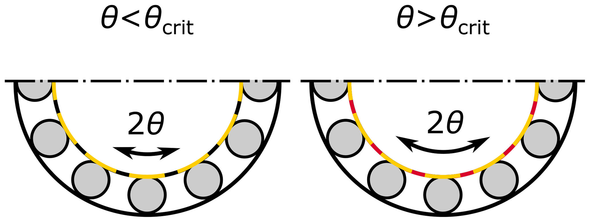
Figure 4 Rumbarger effect: stressed volume on the inner ring as a function of inner ring angle θ relative to ${\mathit{\theta }}_{\mathrm{crit}}={\mathit{\theta }}_{\mathrm{crit},\mathrm{i}}$, for θ<θ_crit and θ>θ_crit. The yellow volume is stressed twice per oscillation cycle (see Fig. 3), and the red volume is stressed four times per oscillation cycle. The black volume is never stressed. Only stress cycles for the inner ring are shown.

For θ<θ_crit, only part of the raceway volume is loaded during operation. For this case, Rumbarger (2003) and Harris et al. (2009) give a load rating that is derived in Appendix A. This derivation makes some simplifications, and Appendix B shows the errors that occur when using Rumbarger's derivation. If applied correctly, the factor (or load rating) should shorten the life of a bearing as compared to Harris¹⁴, though the simplified factor (or load rating) sometimes increases the life for no other reason than the simplifications made in its derivation. The form of Eq. (5) is thus based on Appendix A without any simplifications. Note that since θ_crit differs between the inner and outer races so does a_Rumbarger. Amplitude θ_crit of the outer raceway may be used if a more conservative estimate for the entire bearing is desired¹⁵.

For values of θ≥θ_crit, the simplified approach published in Rumbarger (2003) and Harris et al. (2009) is identical to using the Harris factor. This, too, is merely an approximation: strictly speaking, the life of an unevenly stressed volume (as illustrated in Fig. 4, right-hand side) is not the same as that of an evenly stressed volume which occurs in a rotating bearing¹⁶ (identical to an oscillating bearing with θ=θ_crit) if the total movement of both bearings is the same. Appendix C proposes an extension of the Rumbarger factor for such situations but also concludes that the difference in the factor as compared to a_Harris is almost negligible in most cases. The factor chosen for Eq. (5) thus follows the above-mentioned publications.

The Rumbarger effect does not consider the effects of an uneven load zone on the moving ring, which are covered by Houpert. Moreover, it assumes that no slippage of the rolling-element set occurs, which would move load cycles to occur on different positions of the ring circumference. For a properly installed bearing, Rumbarger and Jones (1968) demonstrated that this assumption can hold true.

2.1.3 Houpert: load zone effects on the moving ring

The Houpert effect was originally covered by Houpert (1999), with a small error in its derivation. This was corrected by Breslau and Schlecht (2020) as well as Houpert and Menck (2021)¹⁷. Aside from the effects also considered by Harris, the Houpert effect considers that the stress cycle history of the moving ring will be different for an oscillating bearing than for a rotating one. This is illustrated in Fig. 5 for an exemplary element on the moving ring.

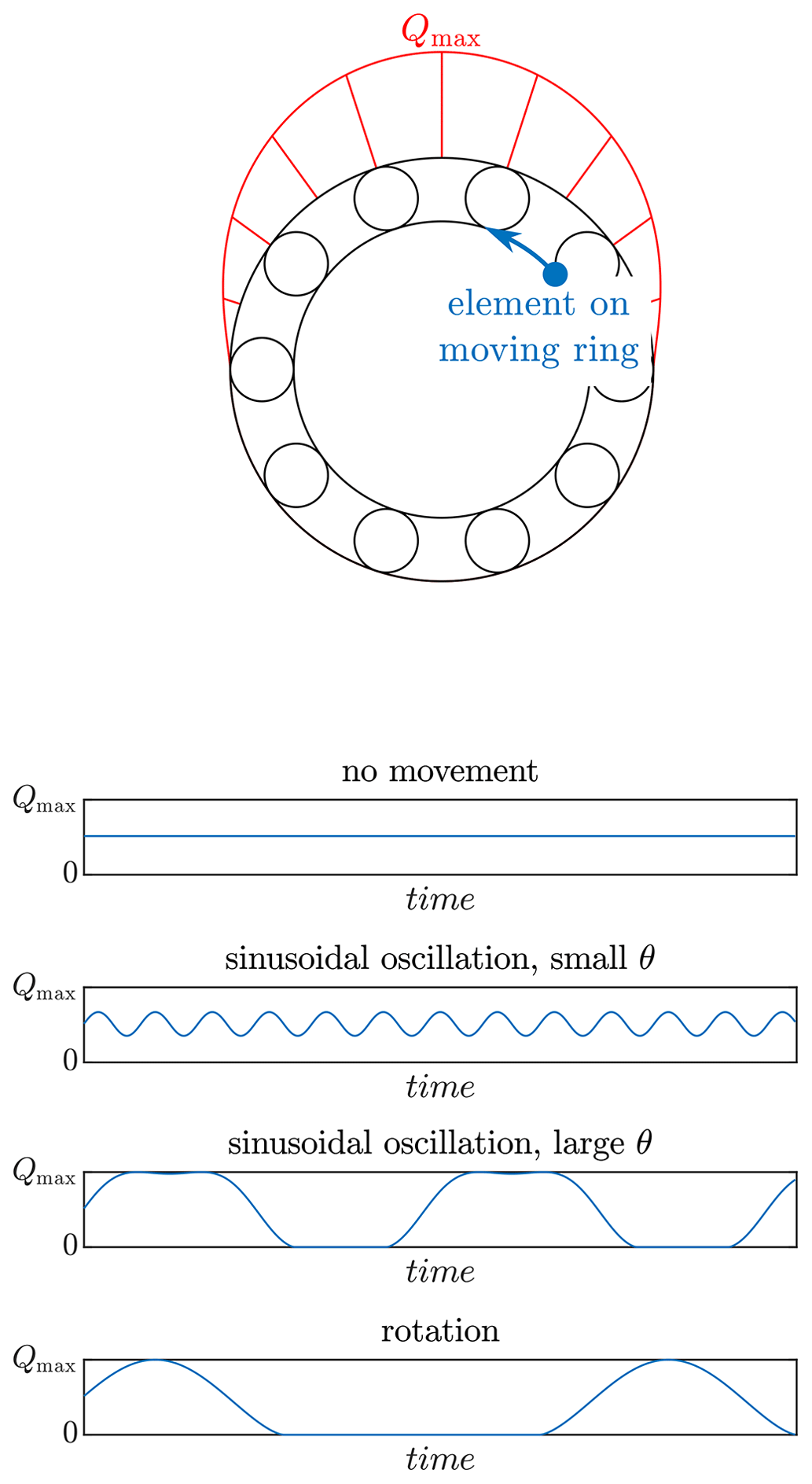
Figure 5 Houpert effect: load history of an exemplary element as a function of movement relative to load zone. Small θ are similar to no movement; large θ are similar to rotation.

In the standard life calculation as pioneered by Lundberg and Palmgren (1947) or used in ISO 281 (ISO, 2007), the load zone is assumed to be constant relative to one ring (called the stationary ring, typically the outer ring). From the viewpoint of Houpert's considerations, movement of the other ring (rotating or oscillating, typically the inner ring) then does not change the load distribution of the stationary ring's raceway. This ring is loaded identically for rotating or oscillating operation. Thus, a_Harris gives the correct life of the stationary ring according to Houpert's derivation.

For the moving ring, however, the Houpert effect predicts a different value to a_Harris. Since Harris merely adjusts the standard (rotation-based) calculation approach by the effect of the difference in traveled distance, they implicitly assume that the effect of the load zone is the same as that in a rotating bearing¹⁸. Thus, a_Harris implicitly assumes an element as depicted in blue in Fig. 5 moves through the entire load zone once for each 360° of movement¹⁹. However, in reality this only applies for oscillations where $\mathit{\theta }=i\cdot \mathrm{180}$° ($\mathit{\phi }=i\cdot \mathrm{360}$°), i=1, 2, 3 …, because for these values of θ each element will move around the entire raceway $\mathrm{2}\cdot \mathit{\theta }=i\cdot \mathrm{360}$ times per oscillation ($\mathit{\phi }=i\cdot \mathrm{360}$ times per oscillation). For very small oscillations θ→0° (φ→0°), on the other hand, the elements increasingly converge toward the stress cycle history seen in a stationary ring²⁰; see Fig. 5. The Houpert factor is generally at or in between the following extreme cases:

$$\begin{array}{}\text{(6)}& \begin{array}{rl}& a_{\mathrm{Houpert}}=\\ & \left\{\begin{array}{ll}{a}_{\mathrm{Harris}}& \mathrm{for}\mathit{\theta }=i\cdot \mathrm{180}\mathrm{with}i=\mathrm{1},\mathrm{2},\mathrm{3},\mathrm{\dots }\\ & \mathrm{or}\mathrm{purely}\mathrm{axial}\mathrm{load}(\mathit{\epsilon }\to \mathrm{\infty })\\ a_{\mathrm{Harris}}\mathrm{in}\mathrm{a}\mathrm{bearing}\mathrm{with}\mathrm{both}\mathrm{rings}& \mathrm{for}\mathit{\theta }\to \mathrm{0}\\ \mathrm{stationary}\mathrm{relative}\mathrm{to}{\mathrm{load}}^{*}& \end{array}\right.\end{array}.\end{array}$$

^* Both rings being stationary relative to load slightly reduces the life as compared to standard calculations (in which one ring is assumed to be rotating) because it increases the equivalent load of the ring which would otherwise be assumed to rotate. It does not affect the factor a_Harris.

In between these extreme cases, detailed calculations have to be performed, curve fits of which can be found in Houpert and Menck (2021). They depend on a value ε, a measure of the load zone size²¹. If applied correctly, the Houpert factor will either be identical to a_Harris in the above given cases or shorten the life of the bearing in all other cases²². The Houpert effect is most noticeable for narrow load zones (small ε) and small oscillation angles θ. Houpert and Menck (2021) find deviations which differ by up to 22 % from those given by the Harris factor for very narrow load zones and small oscillation amplitudes using ISO exponents (see Table A1) and larger deviations of up to 52 % using exponents given by Dominik (1984). This is due to Dominik using a higher Weibull slope of e=1.5. Houpert and Menck (2021) give curve fits to calculate the Houpert factor²³ for ball and roller bearings. If ISO/TS 16281 (ISO, 2008b) is used for the life calculation, the extreme case of small theta (θ→0) can be taken into account by assuming both rings are stationary relative to the load and using a_Harris.

Strictly speaking, the Houpert effect is not independent of the Rumbarger effect, but for its derivations in Breslau and Schlecht (2020) and Houpert and Menck (2021) it is assumed to be.

2.1.4 Other ISO-related approaches and further literature

The above three factors have been covered in a number of publications²⁴, and Breslau and Schlecht (2020) and Houpert and Menck (2021) present the most up-to-date models which include them. Besides the above given publications, there are a number of additional approaches and applications of the above methods. Since all of the above cases are intended for constant oscillation amplitudes, some alternative approaches have been developed which are also intended to be usable for stochastic movement, which leads to different load cycles²⁵ on the bearing rings as depicted in Fig. 2 (blue).

Menck (2023) generalized the Lundberg–Palmgren method to a discrete model (the Finite Segment Method) that can be applied to arbitrary movement. The model applies Eq. (1) to segments of a bearing. The movement of the balls relative to the inner and outer rings for each discrete simulation point is analyzed for potential stress cycles on the respective rings. For each stress cycle N, the variables τ₀, z₀, and V in Eq. (1) are then directly evaluated, and the corresponding damage according to the Palmgren–Miner hypothesis is calculated. The individual survival probabilities of all segments can then be combined into raceway lives, which can be combined into a total bearing life. The model thus encompasses previous use cases and includes the Rumbarger and Houpert effect but can also be used for arbitrary movement and load histories. Menck (2023) shows the model to produce effectively identical results to ISO 281 for simple use cases which are defined by assumptions identical to those of Lundberg and Palmgren (1947) and reproduces results of oscillating bearings from Houpert and Menck (2021) but also applies the model to a rotor blade bearing of a wind turbine.

Hai et al. (2012) propose a generalization of ISO 281 specifically for slewing bearings. They divide the bearing into several segments in a similar way to Menck (2023), but unlike Menck's, their segment width depends directly on the oscillation amplitude. They also make a number of simplifications not made by ISO 281 or Menck²⁶. Their model can be used for individual operating conditions with either rotation or a constant oscillation amplitude; however, several conditions with different amplitudes may also be combined using equivalent loads and equivalent oscillation amplitudes for the segments. They compare their results to an exemplary calculation of NREL DG03 and conclude that their somewhat similar results validate the method. The simplifications make it impossible to establish whether their method is actually more accurate than simply using the oscillation factors given above.

Schwack et al. (2016) do not present a new model but compare factors from Harris, Houpert, and Rumbarger. They also include an approach denoted “ISO”, which is identical to that of Harris. Having published in 2016, the authors also use the erroneous model of Houpert (1999) that was later corrected (see Sect. 2.1.3). Moreover, their application of the Houpert factor is not recommended for double-row bearings with large structural deformation²⁷. Their evaluation of the Rumbarger factor²⁸ results in a longer life than using the Harris factor²⁹. As explained in Sect. 2.1.2, this increase only occurs because of simplifications in the derivations performed by Rumbarger but for no physical reason, since the effects considered should shorten the life, not prolong it. The relatively large deviations from a_Harris shown in Schwack et al. (2016) are therefore both due to inaccuracies in the factors that were used.

Wöll et al. (2018) present a “numerical approach” to calculate the life of a bearing subjected to arbitrary time series. Their model evaluates the life of the whole³⁰ bearing at every discrete time step of the simulation and then calculates the inferred damage according to Palmgren–Miner for every time step, based on the movement that occurred. The model is shown to be identical to a bin count using the Harris factor, see Sect. 2.1.1, for simple sinusoidal movements³¹. For a stochastic time series, their numerical approach produces a shorter life than either Harris's³², Rumbarger's³³, or Houpert's approaches applied to a bin count. Because Wöll et al. (2018) published in 2018, they still use the erroneous Houpert factor from 1999 rather than more recent results (see Sect. 2.1.3); hence, they obtain a longer life with the Houpert factor even though there is no physical reason for such an increase. Furthermore, they compare a bin count using the approaches of Harris, Rumbarger, and Houpert and obtain results that are higher than those of the numerical approach with all three bin count approaches including Harris, and they conclude that using these bin counts “overestimates the lifetime for non-sinusoidal loads and speeds”. It is not possible to assess the accuracy of this statement because their model is based on the life of the whole bearing and thus also includes simplifications as pointed out by Sect. 2.2 of Menck (2023). They also produce a simple method to calculate an equivalent load for oscillating loads, but it fails to take local effects into account as accurately as Menck (2023).

2.1.5 Further effects during oscillation

Further effects occur during oscillation which are not considered by any of the above approaches.

When a rolling element passes completely over a position on the raceway, the orthogonal shear stress below the surface changes from maximum (+τ₀) to minimum (−τ₀) (Lundberg and Palmgren, 1947; Harris and Kotzalas, 2007). This is the typical stress cycle assumed in all ISO-based approaches mentioned here; it is depicted in Fig. 6 on the left. This stress cycle history behaves different in oscillating bearings: for raceway positions close to the reversal points of the oscillation, the direction of the load cycles changes; this phenomenon is depicted in Fig. 6 (oscillation, red case). The shear stress of the volume close to the reversal points does not fully span from +τ₀ to −τ₀ but is stopped prematurely; this too is depicted in Fig. 6 (oscillation, blue case). Similarly, for oscillations with small amplitudes, the stress range does not extend to the maximum and minimum of a passing contact in rotation; see Fig. 6 (small oscillation). None of these effects is considered in the ISO-based approaches (all approaches covered in Sect. 2.1) named herein.

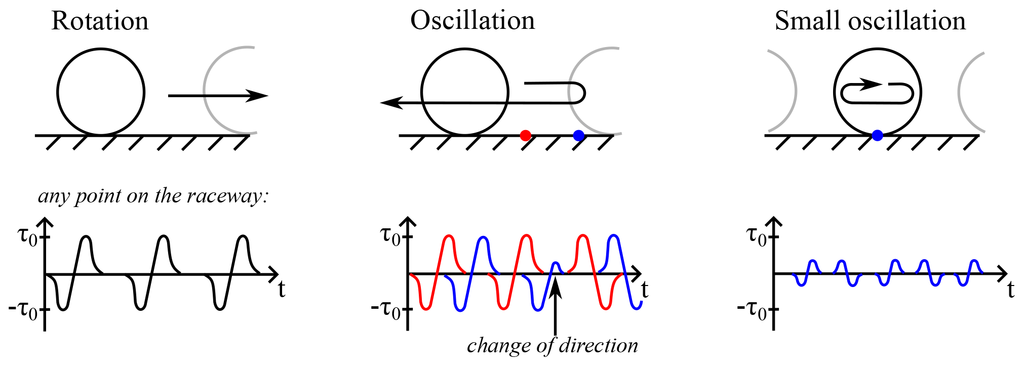
Figure 6 Left: load cycle as assumed by all ISO-based approaches; other examples: further types of load cycles not considered in ISO.

Lubricant film quality is well known to have a significant impact on rolling contact fatigue life (Ioannides et al., 1999; Harris and Kotzalas, 2007). The thickness of the lubricant film is affected by oscillation and may even become so poor that wear rather than fatigue becomes the dominant damage mechanism. Numerous studies investigate wear phenomena in oscillating bearings; for a review, see de La Presilla et al. (2023). As far as the authors are aware, there are no simple models to estimate the thickness of the lubrication film as a function of the oscillation and thus determine its potential effects on rolling contact fatigue. Most bearings are grease-lubricated (Lugt, 2009), including most pitch and yaw bearings (Becker, 2011; Wenske, 2022). Grease consists of, among other things, thickener and base oil (Lugt, 2009). Film thickness estimation would likely become even more challenging with grease lubrication due to the effect of the thickener. Therefore, the effect of lubrication is mostly ignored in all models for rolling contact fatigue calculation in oscillating bearings of which the authors are aware. This statement also applies for the non-ISO-based approaches discussed in Sect. 2.2.

2.1.6 Binning for oscillating bearings

Life calculations often need to be performed for operating conditions that vary over time. As argued in Sect. 2 of Menck (2023), the most accurate way to calculate the rolling contact fatigue life of a bearing under varying operating conditions according to the assumptions in Eq. (1) made by ISO-related approaches is to use the Finite Segment Method according to Menck (2023). This is because the Finite Segment Method considers local load changes rather than summing global, location-independent bearing damage over time. For most users, it will, however, be simpler to remain closer to existing approaches that are based on C and P and do not require a more detailed calculation approach with local damage calculation. Doing so for oscillating bearings necessitates the use of bins representing similar operating conditions in combination with oscillation factors (Harris, Houpert, or Rumbarger). This is the most commonly recommended approach, a version of which is also found, e.g., in the NREL DG03 (Harris et al., 2009). Using bins is merely an approximation when compared to a proper application of Eq. (1) (see Menck, 2023). It is an approximation since the aforementioned factors have all been developed for constant oscillation amplitudes around the same mean position, and they all assume there is a constant load acting on the bearing as it moves, along with a number of other assumptions made by Lundberg and Palmgren (1947), resulting in the life of a whole bearing, a process in which local information is lost.

To apply oscillation factors, movement such as depicted in the stochastical case of Fig. 2 must be translated into bins of oscillations. Typically, variable load is taken into account in fatigue calculations by using rainflow counting (ASTM, 2017) for classical fatigue of structural components. Rainflow counting is also used for the bearing movement (as opposed to the load) for the life calculation of pitch bearings in NREL DG03³⁴, Menck et al. (2020), and Keller and Guo (2022).³⁵ Performing a rainflow count will provide the bins required for further calculations.

The load acting on the bearing is irregular and must be simplified into a single equivalent load P_m for each bin of the cycle count. Ideally, to this end, the equivalent load P_i per time step i is determined, and the equivalent load over the bin P_m is determined from all time steps i=1 … n in the bin as per

$$\begin{array}{}\text{(7)}& {\displaystyle }{P}_{\mathrm{m}}={\left({\displaystyle \frac{N_{\mathrm{1}}{P}_{\mathrm{1}}^p+N_{\mathrm{2}}{P}_{\mathrm{2}}^p+\mathrm{\dots }+N_n{P}_n^p}{N_{\mathrm{1}}+N_{\mathrm{2}}+\mathrm{\dots }+N_n}}\right)}^{\mathrm{1}/p}.\end{array}$$

The value $N_i=n_i\cdot \mathrm{\Delta }{t}_i$ here represents the distance covered in the condition i (measured in degrees or revolutions) and can be calculated from the speed n_i and the time t_i in that condition³⁶. The exponent p is given in Table A1. The approach in Eq. (7) is not specific to oscillation and can similarly be found in various bearing manufacturer catalogs and basic machine element text books (Roloff et al., 1987; Decker, 1995; Haberhauer and Bodenstein, 2001; Liebherr-Components AG, 2017; Schaeffler Technologies AG & Co. KG, 2019).

If it is not possible to determine P_i for each time step, potentially due to the calculation being too costly, it is possible to apply Eq. (7) to the force and moment components contributing to P (including radial force, axial force, and bending moment) and then determine P_m from a suitable function³⁷ based on their values.

Using the P_m values of each bin, it is now possible to calculate the life of each bin $L_{\mathrm{rev}}=(C/P_{\mathrm{m}}{)}^p$. The life in oscillations L_osc according to Eq. (2), using the appropriate factor as determined on the basis of Sect. 4, can be determined too.

All of the bins b=1 … B obtained are then typically combined into one final life using the Palmgren–Miner hypothesis (see also Zaretsky, 1997; Kenworthy et al., 2024) according to

$$\begin{array}{}\text{(8)}& L={\displaystyle \frac{\mathrm{1}}{\frac{{\mathit{\varphi }}_{\mathrm{1}}}{L_{\mathrm{1}}}+\frac{{\mathit{\varphi }}_{\mathrm{2}}}{L_{\mathrm{2}}}+\mathrm{\dots }+\frac{{\mathit{\varphi }}_B}{L_B}}},\end{array}$$

where L₁, …, L_B denote the life in bin b. This may be either the life in oscillations, revolutions, or time. Typically, the life would be in oscillations if oscillation factors have been used, but it may be converted to time or revolutions. L denotes the total combined life of all operating conditions. The variable ϕ gives the proportion of oscillations, revolutions, or time performed in that bin. It is calculated according to

$$\begin{array}{}\text{(9)}& {\mathit{\varphi }}_b={\displaystyle \frac{s_b}{s_{\mathrm{1}}+s_{\mathrm{2}}+\mathrm{\dots }+s_B}},\end{array}$$

where variables s₁, s₂, …, s_b, …, s_B are the oscillations, time, or revolutions that occurred while in that bin but must have the same unit as the lives in Eq. (8). It follows that ${\mathit{\varphi }}_{\mathrm{1}}+{\mathit{\varphi }}_{\mathrm{2}}+\mathrm{\dots }+{\mathit{\varphi }}_B=\mathrm{1}$.

It is worth noting that binning is solely used to reduce the number of data points from real-life data or a simulation. Using modern computers, if there is no hardware-specific necessity to reduce the number of data points, it is possible to use each single step taken from, e.g., an aeroelastic wind turbine simulation or some other data set and treat it as a separate bin to which Eq. (8) is directly applied rather than processing the steps into a reduced number of bins. From the perspective of a proper application of the Palmgren–Miner rule to a whole bearing, usage of each single step is the most accurate approach. It is thus both easier and less error-prone, as well as more accurate than binning beforehand. In order to account for oscillation effects, it would then be required to consider the larger oscillation cycle (amplitude) that a specific step is part of and adjust its life based on that, where the step will typically make up a fraction of the complete oscillation.

2.2 Non-ISO-related approaches

A number of alternative approaches have been developed in recent years, particularly with a focus on blade bearings. Many of these approaches rely on S–N curves that can be determined without testing a complete bearing.

Lopez et al. (2019) propose a model for a blade bearing that uses the movement of the bearing as a basis and computes the multiaxial stress state at the subsurface of the raceway. Loads are obtained from FE simulations using blade root loads from multibody simulations. They apply various multiaxial fatigue criteria and compare the results. They find that IPC (individual pitch control) control strategies significantly increase the damage inflicted on a bearing compared to CPC (collective pitch control) due to the increased movement. The lives calculated with the different fatigue criteria are also sometimes very different from each other.

Leupold et al. (2021) segment a bearing and use a reduced finite element model in a multibody simulation to determine the stress on each segment. Using bearing movement from time series they obtain the number and magnitude of stress cycles for each segment. Individual loads are combined using the Palmgren–Miner hypothesis. Unlike almost all literature on rolling contact fatigue, their model is based on Hertzian normal contact pressure rather than subsurface shear stress. However, they note that “fatigue criteria such as Fatemi–Socie (Fatemi and Socie, 1989) or Dang Van (Dang Van et al., 1989) could also be applied” in subsequent work. They obtain empirical values of the cycles to failure used for the Palmgren–Miner hypothesis from a test of a full-sized blade bearing³⁸ and an assumed slope of the S–N curve from the literature. Further, they note that “a large number of tests are necessary for reliable results” but that “currently, not enough tests have been carried out to determine a reliable service life” with their model.

Hwang and Poll (2022) propose an approach that is then further detailed in Hwang (2023). The approach is based on one circumferential position of the inner bearing ring referred to as “small stressed volume” (SSV). The stress cycle history of different layers below the race at the SSV is analyzed in detail based on the behavior of the inner ring and the load distribution of the bearing. Residual stresses are optionally included in the calculation. For all load cycles that occur, the Palmgren–Miner hypothesis is applied to layers at the SSV. The layer with the lowest survival probability is used to calculate the life of the bearing. To consider the effect of loaded volume, Hwang proposes a simplified method to estimate the loaded volume in the specimens on which their S–N curves are based and the loaded volume in the bearing, as well as to correct the bearing life based on this estimation. The model is applied to rotating and oscillating bearings under constant operating conditions. Hwang (2023) further outlines a proposed application of their model to rotor blade bearings that is not carried out in detail.

Escalero et al. (2023) propose a method for the probabilistic prediction of rolling contact fatigue in multiple-row ball bearings subject to arbitrary load and movement histories. They use a three-dimensionally discretized model of the raceway in which each finite element's individual stress cycle history over time is analyzed using a rainflow count. They use orthogonal shear stress as the governing parameter but note other criteria may be included in the future. The failure probability of the individual elements is determined based on S–N curves obtained from rotating bending specimens and by applying scale factors because of size differences between the specimen and the elements, as well as because of the conversion from normal to shear stress. All individual element failure probabilities are combined using the Weibull weakest link principle (Weibull, 1939). The authors demonstrate their method for a reference case in which a blade bearing was tested (see Sect. 3).

3 Experimental validation

Despite the large number of theoretical models discussed above, there are only a few published experimental results of fatigue tests on oscillating bearings.

Tawresey and Shugarts (1964) tested approximately 750 oil-lubricated bearings under oscillating conditions closely duplicating those encountered in helicopter rotor blade hinges but failed to produce a logical explanation of their results (Rumbarger and Jones, 1968). Rumbarger and Jones (1968) therefore reanalyzed 388 of these bearings comprising 13 test series of identically sized, caged needle-roller bearings and derived a life calculation approach based on the Lundberg–Palmgren theory; see Sect. 2.1.2. They conclude that “the theory of Lundberg and Palmgren is […] favorably compared with the life tests” and derive an experimental load rating C that is shown to be within the bounds defined by the relevant standards at the time (then ASA and AFBMA, today ANSI and ABMA) when adjusted for oscillating motion according to Sect. 2.1.2. Further, they specifically conclude that “the life varied inversely to the fourth power of the radial load”, thus giving p=4, which is identical to the load-life exponent of Lundberg and Palmgren (1952) for the case of pure line contact; see also Table A1. For the 13 test series, they derive Weibull slopes ranging from e=1.13 to 3.55, with a mean value of e=2.04. This is higher than the value of Lundberg and Palmgren (1952) and ISO 281 (ISO, 2007), see Table A1, but they also note that “the wide variation in the values of the Weibull slope are well known”, since different bearing tests routinely produce different Weibull slopes, including even the test data of Lundberg and Palmgren (1952) on which the values of ISO are based; and they note that the higher Weibull slope may be a product of using more modern steels than those used by Lundberg and Palmgren (1952). Despite the tests going as low as an amplitude of θ=1° (φ=2°), none of the bearings show evidence of wear³⁹, but the failed bearings presented “varying degrees of flaking breakout or spalling which is characteristic of failure in rolling contact bearings subjected to rotation”.

FVA (2021) use oil-lubricated cylindrical roller bearings for fatigue tests. They obtain rolling contact fatigue for oscillation amplitudes⁴⁰ as low as θ=1° (φ=2°). The final number of fatigue results is too low to compare them against theoretical calculations, but they conclude that “at least for selected amplitudes, the existing calculation approaches [referring to ISO-based approaches] deliver conservative results compared to the experimentally determined lives”.

Münzing (2017) tests seven ball screws with θ=θ_crit. The lubricant is an aviation grease type Aeroshell 33 MS. The test duration is equivalent to the L₁₀ of the ball screws, which Münzing determines based on the simplified version of the Rumbarger factor found in NREL DG03 (Harris et al., 2009), see Sect. 2.1.2, which they modify⁴¹ to be equal to 1 for θ≥90° (φ≥180°). Five out of seven show initial damage on the raceways. As the standard DIN 631 for ball screws defines a minimum size for surface damage to be considered as fatigue damage and this size is not reached, they are assessed as having passed according to the standard.

Escalero et al. (2023) propose an approach discussed in Sect. 2.2. They compare their results to the test of a single blade bearing under axial load but obtain no correlation. The failure onset in the bearing could not be established exactly as failure already had progressed significantly once it was opened.

Hwang (2023) applies their model to rotating cylindrical roller bearings and angular contact ball bearings as well as four-point bearings. They compare their results to tests of 200 radial cylindrical roller bearings (NU 1006, 55 mm outer diameter) and several double-row four-point bearings of 2.4 m diameter. The model deviates from their experimental results by a factor of about 2 to 10, giving a lower estimate than observed in the tests.

4 Use of the approaches

This section contains recommendations for selection of a rolling contact fatigue life calculation approach. Section 4.1 contains a number of general recommendations, Sect. 4.2 and 4.3 discuss some simple illustrative examples, and Sect. 4.4 and 4.5 detail possible uses for a pitch and yaw bearing in a wind turbine.

4.1 Recommendations for use

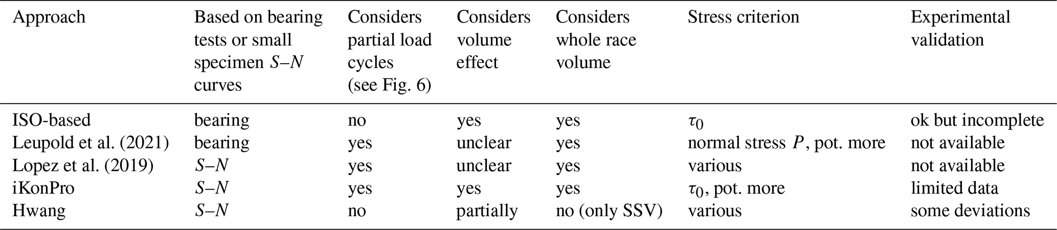
A flowchart of when to use which rolling contact fatigue life calculation approach, based on the underlying modeled physical principles, is given in Fig. 7. Theoretically, the conditions in the flowchart must hold all the time. Practically, it will be sufficient if they hold most of the time. Dashed arrows represent mathematical approximations, which are considered less accurate than exact calculations. For the ISO-related approaches, recommendations are given according to the underlying physical phenomena considered in the derivations as described in this paper. The recommendations herein may therefore deviate from those given by the respective authors. For the non-ISO-related approaches, recommendations generally follow the respective authors since they rely on less widely acknowledged approaches and may therefore be subject to the more individual interpretation of the respective authors. Further comparisons between the approaches are given in Table 1.

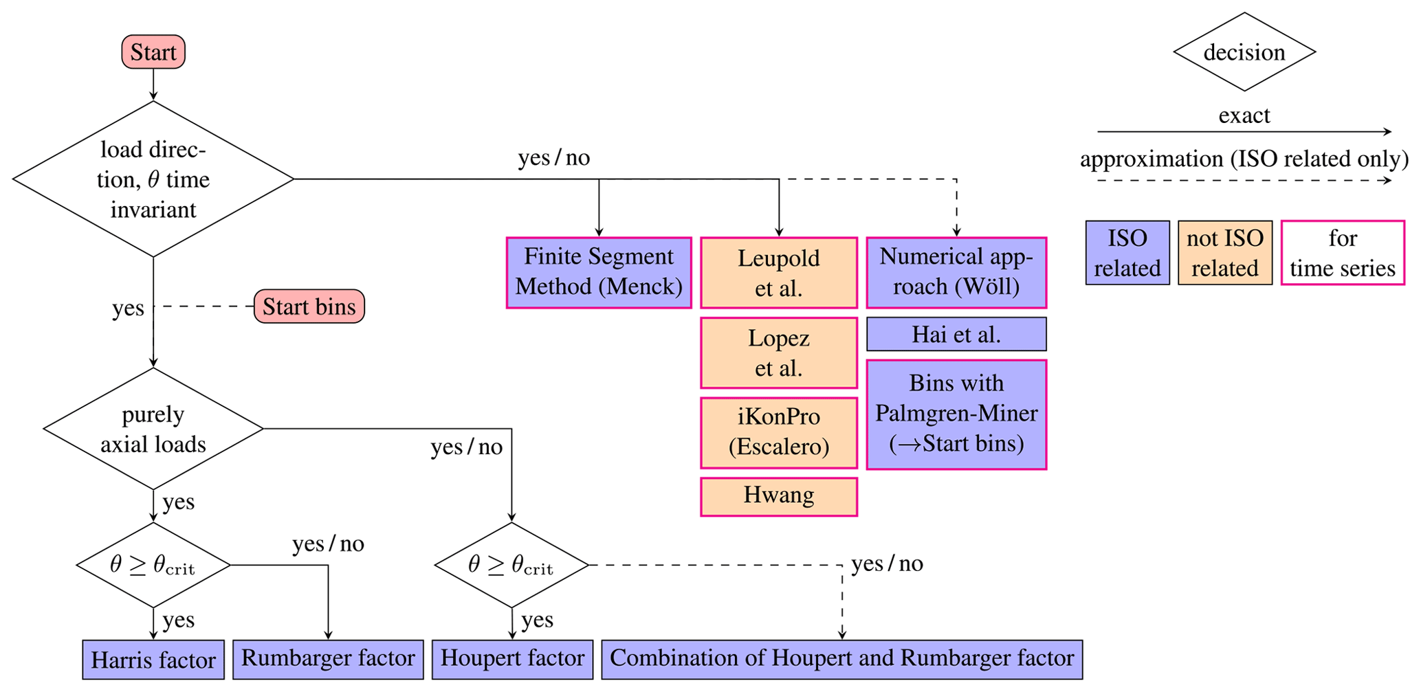
Figure 7 Flowchart to find the simplest applicable life calculation approach for a given oscillating bearing.

Leupold et al. (2021)Lopez et al. (2019)

Table 1 Comparison of different life calculation approaches.

Generally, the start of the flowchart is given by the “Start” box. If bins are used (see Sect. 2.1.6), the “Start bins” box can be used for an approximation. In this case, the condition θ≥θ_crit applies if all circumferential positions of the ring experience some stress cycles over all bins⁴².

For general users seeking to apply a life calculation, ISO-related approaches are preferred to non-ISO-related ones due to their simplicity and the fact that there is much more empirical basis underlying them. In the event of an invariant load direction and oscillation amplitude θ, various methods are shown in the figure. Among the ISO-related ones, that by Menck can be considered to be most accurate; however, it is also complicated to apply. A less accurate (i.e., an approximated) but simpler method will be most useful for most readers. Among the approximated ISO-related methods for an invariant load direction and θ, “Bins with Palmgren–Miner” is the recommended approach due to its wide use in many areas. Among the non-ISO-related methods, Table 1 gives an overview of advantages and disadvantages of each method. Since only users with very specific aims will refer to these methods, it is up to readers to make their own decision as to which of these methods, if any, to use.

None of the ISO-related approaches predicts huge deviations from a_Harris for regular operating conditions. For a rough estimate, if the desired life is well below that calculated with the Harris approach, it is very likely to pass with the other ISO-related approaches, too. For a more precise calculation, narrow load zones or small oscillation angles below θ_crit will produce the largest deviations from the Harris factor.

For the Rumbarger effect, based on Sect. 2.1.2 and Appendix A, the flowchart recommends combining this effect with the Houpert effect for non purely-axial loads (i.e., radial and moment loads). This deviates from Rumbarger and Jones (1968), where the Rumbarger effect is used without consideration of the Houpert effect for radial bearings, and Harris et al. (2009), where the Rumbarger effect is used without consideration of the Houpert effect for moment loads, but this recommendation is based on the fact that particularly for these cases which represent relatively small load zones ε, the Houpert effect is to be taken into account⁴³.

The flowchart considers the numerical approach of Wöll et al. (2018) and Hai et al. (2012) to be approximations. Although Wöll et al. (2018) use the approach for a series of stochastic movements and load directions, they also note “the numerical approach lacks the capability of taking sophisticated distinctions into account, as [Rumbarger]⁴⁴ does with the critical angle distinction and Houpert does with comparing the oscillation amplitude to the load zone size”. The reason their method cannot consider these local effects is due to the global application of the Palmgren–Miner hypothesis; see Menck et al. (2022), Sect. 2.2. Menck's Finite Segment Method can be seen as a more accurate (but more difficult to implement) version of Wöll's numerical approach that considers local effects also seen with Houpert and Rumbarger. Wöll's numerical approach is also effectively identical to a bin count, listed below it in the flowchart. Hai et al. (2012) is listed as an approximation due to the reasons set out in Sect. 2.1.

As noted in Appendix C, the Rumbarger effect actually applies even for oscillation amplitudes θ>θ_crit, but since its effect is so small at these amplitudes the effect at larger amplitudes is not considered in Fig. 7.

Some approaches are derived in different sources. The authors recommend using the following sources: the Harris factor is given in Sect. 2.1.1. The Houpert factor is best considered according to the model of Breslau and Schlecht (2020) or Houpert and Menck (2021). The latter reference includes curve fits for ease of use. Older references may be erroneous. The Rumbarger effect is best calculated according to Eq. (5) or Breslau and Schlecht (2020) or Houpert and Menck (2021); see also Sect. 2.1.2. Older references may be oversimplified. A combination of the Houpert factor and the Rumbarger factor is best performed according to Breslau and Schlecht (2020) and Houpert and Menck (2021). All other approaches in the flowchart are best performed according to the publications of their respective authors.

4.2 Application to a Cardan joint bearing

An exemplary Cardan joint connects two shafts whose axes are inclined to each other. The shafts rotate, causing the Cardan joint bearing to oscillate with a constant oscillation amplitude of θ=5°. The exemplary bearing is a radial bearing with contact angle α=0°. It contains Z=15 balls with a diameter of D=10 mm and has a pitch diameter of d_m=60 mm. The critical amplitude according to Eq. (4) is then ${\mathit{\theta }}_{\mathrm{crit},\mathrm{o}}=\mathrm{28.8}$° and ${\mathit{\theta }}_{\mathrm{crit},\mathrm{i}}=\mathrm{20.6}$° for the outer and inner raceways, respectively. The load zone is made up of a purely radial load that is constant with respect to the outer ring. Half the circumference is loaded, giving ε=0.5, and inner and outer ring osculation are identical.

In the context of Fig. 7, both the load direction and θ are thus time invariant. There is no purely axial load, and θ≥θ_crit does not apply. A combination of the Houpert and Rumbarger factors can thus be used by multiplying them as shown in Houpert and Menck (2021), using the Rumbarger factor for the outer race to be conservative. Alternatively, the approach given by Breslau and Schlecht (2020), who discussed Cardan joint bearings in their paper in more detail, may be used. Furthermore, the other approaches in the top right of Fig. 7 may also be used since they apply to general time-series-based data and thus also apply to simpler data.

The Harris factor for this bearing is a_Harris=18 according to Eq. (3). The Rumbarger factor according to Eq. (5) is a_Rumbarger=15.1 if the outer ring is assumed to be conservative; it would be 15.6 for the inner ring. A combination of the Rumbarger and Houpert effect is calculated according to Houpert and Menck (2021) as⁴⁵ a_osc=14.2. This final value is recommended here because it accounts for both relevant effects that occur in the bearing described above. It is smaller than the Harris factor alone and also smaller than the Rumbarger factor alone, since the effects of both Rumbarger and Harris decrease life.

4.3 Application to a crane slewing bearing

An exemplary crane slewing bearing is located at the bottom of a crane which is exclusively used to perform oscillation amplitudes of θ=90° to unload a ship. It is an axial bearing with α=90°. The critical amplitude according to Eq. (4) is θ_crit=8° for both inner and outer rings. The load is mostly an axial load with only a slight tilting moment component. According to Fig. 7, the load direction is then invariant, and so is the oscillation amplitude θ. The load is (approximately) purely axial, and θ>θ_crit. Therefore, the Harris factor applies for this bearing. For the amplitude of θ=90°, a_Harris=1.

The Rumbarger factor according to Eq. (5) would be equal to a_Harris due to θ>θ_crit. The Houpert factor according to Eq. (6) is approximately a_Houpert≈a_Harris due to the mostly axial load giving a large ε≫1. This is why it is valid to simply use a_Harris for the given case.

If θ were time invariant, it would also be possible to use the Harris factor and combine different bins using the generalized mean in Eq. (7). Again, more complicated approaches in the top right of the flowchart would also apply.

4.4 Application to rotor blade bearings

A number of publications include rolling contact fatigue calculations for rotor blade bearings, some ISO-related⁴⁶ (see Harris et al., 2009; Schwack et al., 2016; Menck et al., 2020; Keller and Guo, 2022; Menck, 2023; and Rezaei et al., 2023) and some not (see Lopez et al., 2019; Leupold et al., 2021; Escalero et al., 2023; and Hwang, 2023). The non-ISO-based methods are, as stated in Sect. 4, best applied according to the respective publications given above, though many of these publications are relatively short and likely not sufficient for an end user to actually copy their technique and apply to an actual bearing. Moreover, according to Sect. 3, the experimental validation for these models is still lacking. Therefore, this section will focus on ISO-based approaches, which remain the most common life calculation methods for rolling contact fatigue.

Rotor blade bearings typically experience pitch amplitudes as in the stochastic case depicted in Fig. 2: their oscillation amplitude is irregular, as are the loads acting on the blade in five degrees of freedom. Moreover, the load direction changes due to the blade weight bending moment as the blade rotates and the blade aerodynamic bending moment that varies with the turbine operating conditions (Menck et al., 2020). Therefore, according to Fig. 7, the Finite Segment Method (Menck, 2023) would be the most appropriate ISO-based method for an engineer to use. However, some simplified approaches exist, too. These include the methods by Wöll et al. (2018) and Hai et al. (2012), as well as the approach most often chosen by users, a bin count. Using a bin count is likely the most user-friendly and well known of the approaches. Section 2.1.6 details how to do a bin count and therefore represents the first step required for calculating the life of a pitch bearing, and this step is described in detail below.

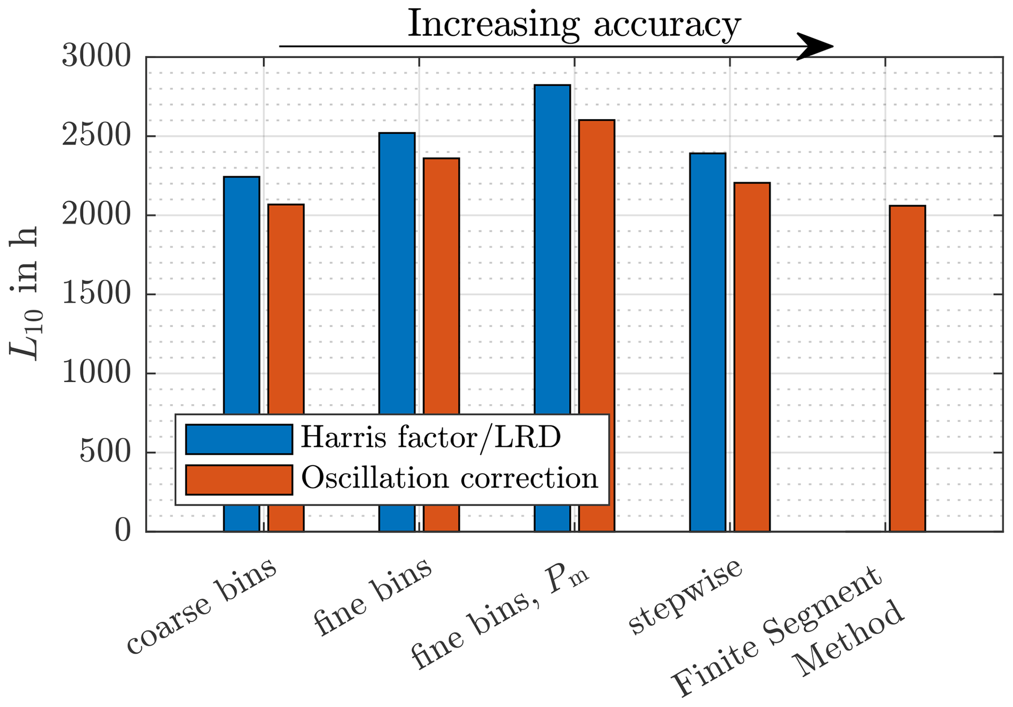
Figure 8 Comparison of the different approaches in Table 2 with the Harris factor and additional effects for oscillation considered.

At this point we assume bins to be present where ideally no binning is performed but each time step of the simulation is used as an individual bin (see Sect. 2.1.6). Prior to the application of Eq. (8), the lives L_b of each bin must be calculated using an approach which takes the oscillation into consideration. To this end it is useful to refer to Fig. 7. Although both the load direction and pitch angle θ are time invariant, they have to be considered to be approximately constant in order to use oscillation factors, hence the start at “Start bins”. The loads are not purely axial, but the oscillation of the bearing – over the entire operating time of the turbine – is large enough to have rolling elements cover the entirety of the raceway at one point or another^{47, 48}. That is to say there is no area that is never stressed, giving θ>θ_crit. The Houpert factor is therefore a useful factor to employ, whereas the Rumbarger factor is not, since each segment of the raceway will see rolling elements pass by fairly regularly.⁴⁹

Using ISO/TS 16281, there are two different equivalent loads: Q_ei for the inner ring and Q_ee for the outer ring. For each of these rings, users must decide whether the ring is rotating or stationary relative to the load. Since rotor blade bearings mostly perform small oscillations below approximately 20° of amplitude, an alternative to using the Houpert factor is to use the equivalent load of a stationary ring for both rings in combination with the Harris factor (see Sect. 2.1.3). This is equivalent to the worst-case scenario of the Houpert factor and is almost identical to it at small oscillation amplitudes.

Menck et al., 2020Menck, 2023

Table 2 Different approaches to calculate the life of a rotor blade bearing.

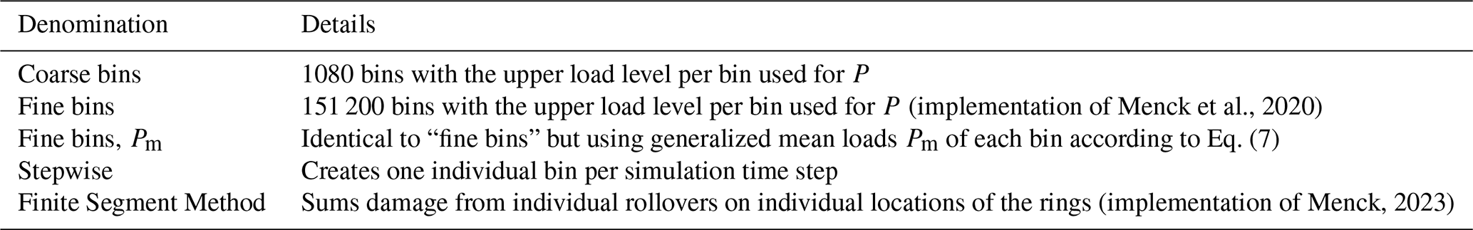
Figure 8 shows different approaches to calculate the life of a rotor blade bearing using data from aeroelastic simulations. Table 2 summarizes the approaches. The five approaches are ordered with increasing accuracy to the right of the figure, where “increasing accuracy” means that the Palmgren–Miner hypothesis is applied as accurately as possible. All of them are closely related to ISO and therefore to Eq. (1). The first three approaches (name containing “bins”) all pre-process the time series data into bins based on the bearing movement and load data acting in a given time step. The fourth approach (stepwise) uses each individual time step of the simulation as a separate bin. The fifth method (Finite Segment Method) does not use binning but directly calculates damage based on the number of rollovers occurring in segments of the ring. This is the most accurate method and can be used as a reference for the others. Results for the first four methods have been obtained using ISO/TS 16281 for the equivalent load. All results are displayed using the Harris factor, if applicable (that is, if bins were used in some form), assuming one ring to be rotating in ISO/TS 16281 and using a more accurate method for oscillation, which means that both rings have been calculated as stationary according to ISO/TS 16281 in combination with the Harris factor. The Finite Segment Method automatically includes effects of oscillation and cannot be used with the Harris factor.

The first three approaches shown in Fig. 8 involve pre-processing into bins. It can be seen that some of their results deviate more and some deviate less from the Finite Segment Method. These results are heavily dependent on details of the pre-processing used for the data, and the results shown here are not representative for other potential types of pre-processing. The fact that the “coarse bins” simulation using an oscillation correction is so close to the Finite Segment Method is thus likely accidental and not because this particular approach is particularly representative of a more correct method.

Comparing the life L_10,stepwise of the stepwise calculation where one ring is assumed to be stationary and one is assumed to be rotating (Harris factor/LRD) to the results L_10,FSM of the more accurate Finite Segment Method, one can see that

$$\begin{array}{}\text{(10)}& L_{\mathrm{10},\mathrm{FSM}}=\mathrm{0.86}\cdot L_{\mathrm{10},\mathrm{stepwise}}.\end{array}$$

This is roughly in line with using the Houpert factor or assuming both rings to be stationary, which gives a result which is only slightly higher (see Fig. 8, stepwise, oscillation correction). The result of the Finite Segment Method is slightly lower because it first sums local damage over the entire span of the simulation before determining the global bearing life. Therefore, load concentrations on individual segments and bearing rings are considered more accurately than with the other methods⁵⁰. For calculations performed with ISO-related approaches using binning of data in some form, where one ring is assumed to be stationary and one is assumed to be rotating⁵¹, it is therefore reasonable to expect a life which is 10 % to 15 % longer than that obtained with more advanced methods. Further deviations that are caused by binning of the data and other forms of pre-processing are impossible to predict, and therefore a stepwise calculation is preferable.

4.5 Application to yaw bearings

For yaw bearings, the oscillation behavior is highly site dependent. Any wind direction history can be calculated using the Finite Segment Method or the other approaches highlighted with thick borders in Fig. 7. For the design of a wind turbine, yawing movements are seldom simulated, apart from a few design load cases (Wenske, 2022). Rather, constant offsets from an optimal yawing position are simulated and assumed to be present for a certain amount of operating time. Yaw movement is then assumed to be distributed among these simulated cases. Since detailed time series will typically not be available, binning will often be necessary in order to calculate the life, though detailed time series would be preferable, if available.

Though the behavior is highly dependent on both the site of the turbine as well as the design of the yaw system, some general statements can be made. Firstly, even at sites with only one main wind direction, it is likely that this wind direction will vary by a few degrees. Secondly, the yaw misalignment that triggers a yaw movement is dependent on the yaw system design. Yaw misalignments of 3 to 8° are common, realistic values (Wenske, 2022). Finally, the design of large-scale yaw bearings, like that of pitch bearings, usually includes a large number of rolling elements in excess of 50 or even 100 and more per row⁵², giving small critical angles θ_crit. It is thus unlikely that any yaw bearing will be operated in a manner whereby during the entire operating history of the bearing the loads are truly concentrated only on parts of the raceway, since that would require yaw movements to be consistently smaller than θ_crit despite fluctuations in the wind direction and possible slippage of the rolling-element set. The Rumbarger effect is thus unlikely to be relevant for yaw bearings in the field.

Regarding the Houpert effect, the wind direction is important. Unlike for typical bearings, the rotating (oscillating) ring is the one that will always be loaded in one primary position since it is consistently moved toward the wind. The stationary ring, on the other hand, can experience very concentrated loads in one position (in the case of a site with only one main wind direction) or it can even experience loads spread evenly over its circumference (on sites with no clear main wind direction, where the wind can come from any direction). In the first case (one main wind direction only), similar to pitch bearings, both rings experience a high concentration of loads in one spot. It is thus recommended that the Houpert effect is considered, ideally by using the equivalent load for a stationary ring, for the calculation of both Q_ei and Q_ee if ISO/TS 16281 is used. Otherwise, the Houpert effect can be taken into account by using the publications mentioned in Sect. 4.1. Assuming one main wind direction is the more conservative assumption and should be the approach to choose in case of doubt. Since yaw bearings, like pitch bearings, are strongly affected by a tilting moment, each of their raceways is commonly loaded around half of its circumference (Chen and Wen, 2012; Schwack et al., 2016; Menck et al., 2020; Graßmann et al., 2023), corresponding to a load zone parameter (see Sect. 2.1.3) of ε=0.4 … 0.6. With this value of ε, a life which is around 10 % shorter than that obtained with the Harris factor is to be expected for small oscillation amplitudes (Houpert and Menck, 2021). If the main wind direction is truly evenly spread over all compass directions, it is permissible to use the equivalent load of a ring that rotates relative to the load for the outer ring, approximately equivalent to simply using the Harris factor for the entire bearing⁵³.

5 Current challenges and critical future work

While there are a number of different approaches for the calculation of rolling contact fatigue in oscillating bearings, the validation of these models is lacking to a large extent. Among the ISO-related approaches, some experimental results suggest that the predictions may be accurate, as discussed in this paper. One can also argue that the ISO-related approaches, being based on the widely accepted standard ISO 281, are partially validated by the rotating bearings which were used to validate the standard in itself.

For regular operating conditions, the ISO-related approaches do not differ by a huge margin. Validation of one approach therefore also increases the likelihood that another of the ISO-related ones is accurate. Potential attempts to validate these bearings can focus on the different phenomena that are covered by the Houpert and the Rumbarger effect to validate them independently of each other, but as they are based on the same foundation, these validations (if successful) will have a positive effect on each other, too.

A number of publications have shown deviations of rotating bearing lives from the ISO standard (Harris and Kotzalas, 2007; Londhe et al., 2015). A validation of the ISO-related models in this paper should therefore take into account that they are relative values. Any bearings used for oscillating tests should ideally also be used for rotating tests in otherwise identical or similar conditions, to ensure that potential deviations from the results shown in this review are not simply due to the bearings themselves lasting longer than suggested by the standard but actually due to the relative factors given here being inaccurate.

All of the models – ISO-related and non-ISO-related alike – completely neglect the influence of lubrication. This is probably the grossest simplification and the biggest uncertainty underlying all models discussed in this review. Lubrication is a complicated topic that is often simplified. Even for regular bearings, over 90 % of bearings are grease-lubricated (Lugt, 2009), but for the life calculation the grease behavior is mostly approximated using base oil properties even though grease is well known to behave differently (Lugt, 2012). For oscillating applications, due to the movement-dependent lubrication film (Venner and Hagmeijer, 2008), this issue becomes much more complex than for rotating bearings, hence why all models in this review simply neglect the topic completely.

While this review and many publications before it (Harris et al., 2009; Schwack et al., 2016; Menck, 2023) applied ISO-related methods to large slewing bearings, there have been publications suggesting (without evidence) that the ISO standard does not apply for pitch and yaw bearings (Potočnik et al., 2010; Lopez et al., 2019). Whether or not this is the case is another topic worth researching. The non-ISO-related methods in this review present an alternative approach to life calculation for people who distrust the ISO standard, but the evidence proving their aptitude is, to date, lacking to a much greater extent that of the ISO-related models. While it is possible that large oscillating slewing bearings behave differently than suggested in this review, it is also an option to introduce corrective factors or change load rating and equivalent load in order to perform a standard calculation for large oscillating slewing bearings nonetheless.

6 Conclusions

This work has given an overview of the literature on rolling contact fatigue calculation for oscillating bearings. Many approaches are based on ISO, tend to be user friendly, and are often applied in the literature. Most of these approaches have been proposed and used in the literature without an explanation as to when they apply. The aim of this paper was to explain when which approach can be applied. It is worth noting that many older publications, particularly for the Rumbarger effect and the Houpert effect, include errors or simplifications, and hence more recent publications, including this one, are to be preferred as a source. When applied correctly according to more recent literature and for standard operating cases, the deviations between Harris, Rumbarger, and Houpert as well as other ISO-based approaches are typically not huge. This also applies to the operating conditions of pitch and yaw bearings. The large deviations obtained with alternative approaches to the Harris factor that are seen in some publications are often due to errors or simplifications. All ISO-based approaches shorten the calculated life compared to the Harris factor (or are identical to it) if applied correctly. This is because all ISO-based approaches that deviate from Harris do so because they either incorporate the Houpert or Rumbarger effect, or both, and both of these effects cause either the same life or a reduction in life compared to the Harris factor if applied correctly. Currently published ISO-based calculation approaches that increase life compared to the Harris factor are erroneous, potentially due to being overly simplified. Some phenomena described in this paper that have not yet been analyzed in the literature could slightly increase lives even for ISO-based methods.

Aside from these commonly used factors, a number of alternative approaches have been discussed. These include some ISO-related ones and some approaches that deviate significantly from ISO. Many of these alternative approaches, including ISO-related and non-ISO-related ones, have been designed particularly for rotor blade bearings.

The experimental validation of all models in the literature is relatively poor. Some experimental results from the ISO-based approaches compared well with the calculated life, suggesting that the predictions of ISO-based methods may be relatively close to the actual life, while validations of the alternative approaches are mostly lacking.

This work may help engineers identify which approach to use for the rolling contact fatigue life calculation for a given oscillating bearing. It has been written with a particular focus on wind turbine slewing bearings but may also be used as a reference for any other oscillating bearings in other industrial sectors.

Appendix A: Derivation of the Rumbarger factor

Lundberg and Palmgren (1947) state, using Eq. (1) and knowing that N=uL,

$$\begin{array}{}\text{(A1)}& \ln {\displaystyle \frac{\mathrm{1}}{S}}\propto {\displaystyle \frac{{\mathit{\tau }}_{\mathrm{0}}^{\mathrm{c}}(uL{)}^e}{z_{\mathrm{0}}^h}}V,\end{array}$$

where τ₀ is the maximum shear stress and z₀ its depth under the raceway, V is the loaded volume, and u gives the stress cycles per million oscillations or revolutions L. For a constant survival probability S, it follows that

$$\begin{array}{}\text{(A2)}& L\propto {\left({\displaystyle \frac{z_{\mathrm{0}}^h}{{\mathit{\tau }}_{\mathrm{0}}^{\mathrm{c}}V}}\right)}^{\mathrm{1}/e}{u}^{-\mathrm{1}}.\end{array}$$

Comparing two identical bearings under identical τ₀ and z₀, one oscillating and one rotating, for θ<θ_crit, where $V_{\mathrm{osc}}/V_{\mathrm{rot}}=\mathit{\theta }/{\mathit{\theta }}_{\mathrm{crit}}$ we obtain

$$\begin{array}{}\text{(A3)}& a_{\mathrm{prt}}={\displaystyle \frac{L_{\mathrm{osc}}}{L_{\mathrm{rot}}}}={\displaystyle \frac{u_{\mathrm{rot}}}{u_{\mathrm{osc}}}}{\left({\displaystyle \frac{\mathit{\theta }}{{\mathit{\theta }}_{\mathrm{crit}}}}\right)}^{-\mathrm{1}/e}.\end{array}$$

This is equivalent to Eq. (18) given by Breslau and Schlecht (2020). In their Eq. (19), using θ_crit from Eq. (4), they then go on to derive⁵⁴

$$\begin{array}{}\text{(A4)}& a_{\mathrm{prt}\mathrm{i},\mathrm{o}}={\displaystyle \frac{Z(\mathrm{1}\pm \mathit{\gamma })}{\mathrm{4}}}{\left[{\displaystyle \frac{\mathit{\theta }Z(\mathrm{1}\pm \mathit{\gamma })}{\mathrm{360}\mathit{°}}}\right]}^{-\mathrm{1}/e},\end{array}$$

with the minus (−) sign referring to the outer and the plus (+) sign to the inner raceway. Using a_Harris from Eq. (3), this can be rewritten as done by Houpert and Menck (2021):

$$\begin{array}{}\text{(A5)}& a_{\mathrm{prt}\mathrm{i},\mathrm{o}}={\left({\displaystyle \frac{\mathit{\theta }}{{\mathit{\theta }}_{\mathrm{crit}\mathrm{i},\mathrm{o}}}}\right)}^{\mathrm{1}-\mathrm{1}/e}{a}_{\mathrm{Harris}}.\end{array}$$

Both Rumbarger and the NREL DG03 (co-authored by Rumbarger) use a different amplitude definition than in this paper, defined by φ=2θ. Equation (A4) then becomes

$$\begin{array}{}\text{(A6)}& \begin{array}{rl}{a}_{\mathrm{prt}\mathrm{i},\mathrm{o}}& ={\displaystyle \frac{Z(\mathrm{1}\pm \mathit{\gamma })}{\mathrm{4}}}{\left[{\displaystyle \frac{\mathit{\phi }Z(\mathrm{1}\pm \mathit{\gamma })}{\mathrm{720}\mathit{°}}}\right]}^{-\mathrm{1}/e}\\ & =\underset{f_{\mathrm{Rum}}}{\underbrace{(\mathrm{1}\pm \mathit{\gamma }{)}^{\mathrm{1}-\mathrm{1}/e}{\mathrm{4}}^{-\mathrm{1}+\mathrm{1}/e}}}{Z}^{\mathrm{1}-\mathrm{1}/e}{\left[{\displaystyle \frac{\mathit{\phi }}{\mathrm{180}\mathit{°}}}\right]}^{-\mathrm{1}/e}.\end{array}\end{array}$$

The factor f_Rum is introduced here to include the terms (1±γ) and ${\mathrm{4}}^{-\mathrm{1}+\mathrm{1}/e}$, both of which Rumbarger assumes to be approximately 1. Thus, Rumbarger obtains f_Rum≈1. In order to keep track of the error introduced by this assumption, f_Rum will be retained in the following equations.

Rumbarger does not adjust life by using a factor but by changing the load rating. A factor can be converted to an equivalent load rating using

$$\begin{array}{}\text{(A7)}& L_{\mathrm{10},\mathrm{prt}}=a_{\mathrm{prt}}{\left({\displaystyle \frac{C}{P}}\right)}^p={\left({\displaystyle \frac{a_{\mathrm{prt}}^{\mathrm{1}/p}C}{P}}\right)}^p={\left({\displaystyle \frac{C_{\mathrm{Rum}}}{P}}\right)}^p,\end{array}$$

with Eq. (A6) used for the adjusted Rumbarger load rating,

$$\begin{array}{}\text{(A8)}& C_{\mathrm{Rum}}=a_{\mathrm{prt}}^{\mathrm{1}/p}C={\left(f_{\mathrm{Rum}}{Z}^{\mathrm{1}-\mathrm{1}/e}{\left[{\displaystyle \frac{\mathit{\phi }}{\mathrm{180}\mathit{°}}}\right]}^{-\mathrm{1}/e}\right)}^{\mathrm{1}/p}C.\end{array}$$

Equation (A8) is identical to the load ratings given in Rumbarger (2003) and Harris et al. (2009) when assuming f_Rum=1 and using the parameters given in Table A1.

The error can simply be corrected by using either Eq. (A8) or Eq. (A6) separately for each raceway (see Breslau and Schlecht, 2020) and without assuming f_Rum=1.

Table A1 Exponents c, e, h, and p according to ISO.

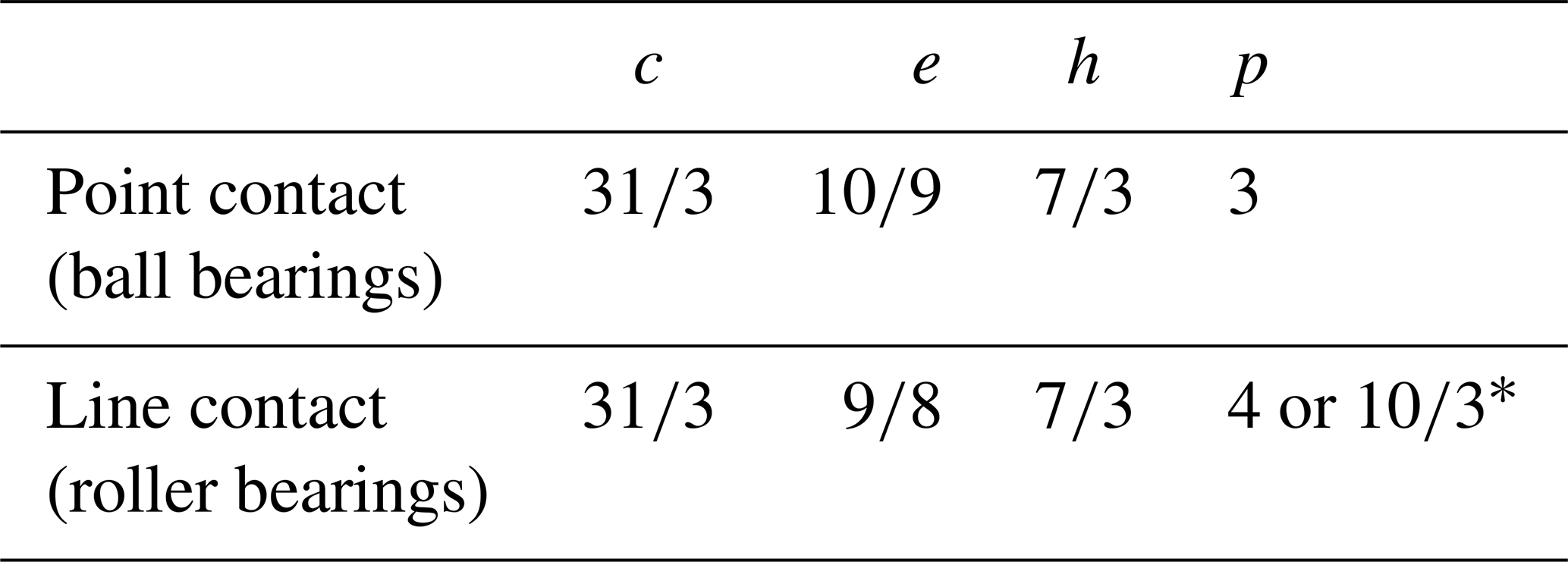
^* Exponent p=4 follows from the given c, e, and h and is consequently used by Rumbarger (2003) and Breslau and Schlecht (2020) in their derivations. Nonetheless, ISO 281 uses $p=\mathrm{10}/\mathrm{3}$ in calculating $L={\left(\frac{C}{P}\right)}^p$. This is explained in Lundberg and Palmgren (1952) and ISO (2021), which argue for the choice of $p=\mathrm{10}/\mathrm{3}$ because in some load cases line contact within roller bearings may turn into point contact. Thus, p=4 for detailed calculations of rolling contact fatigue where line contact is sure to take place, and $p=\mathrm{10}/\mathrm{3}$ for calculations by general users applying $(C/P{)}^p$.

Appendix B: Error of the Rumbarger factor for θ<θ_crit

By assuming $(\mathrm{1}\pm \mathit{\gamma })\approx \mathrm{1}$, Rumbarger effectively neglects the difference between inner and outer races and obtains an equation which can be used for the entire bearing. The assumption ${\mathrm{4}}^{-\mathrm{1}+\mathrm{1}/e}\approx \mathrm{1}$, on the other hand, is an unnecessary simplification that leads to errors, as will be seen in the following.

B1 Error on one raceway

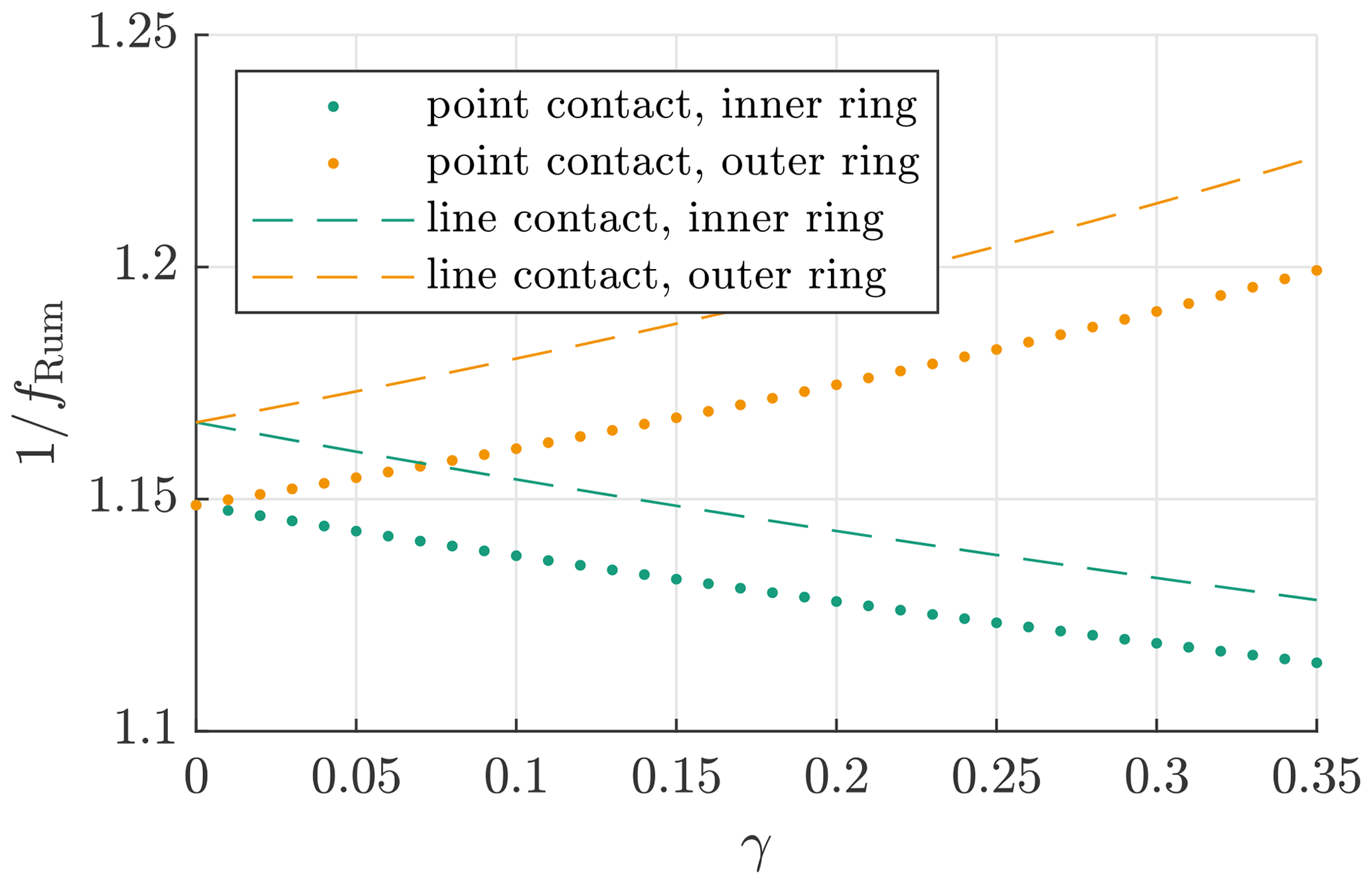
The error of Rumbarger's assumptions for one single raceway can be easily calculated by comparing the life L_10,prt from Eq. (A7) that, correctly, assumes f_Rum≠1 to that which approximates f_Rum=1 as done by Rumbarger.

$$\begin{array}{}\text{(B1)}& {\displaystyle \frac{L_{\mathrm{10},\mathrm{prt}}\left(f_{\mathrm{Rum}}=\mathrm{1}\right)}{L_{\mathrm{10},\mathrm{prt}}\left(f_{\mathrm{Rum}}\ne \mathrm{1}\right)}}={\displaystyle \frac{\mathrm{1}}{f_{\mathrm{Rum}}}}\end{array}$$

Values of $\mathrm{1}/f_{\mathrm{Rum}}$ for point and line contact as well as different values of γ are depicted in Fig. B1. One can see that C_Rum consistently overestimates the actual life, up to 23 % for γ=0.35 on a roller bearing's outer ring. The error is dominated by Rumbarger's neglect of the factor ${\mathrm{4}}^{-\mathrm{1}+\mathrm{1}/e}$, which is 0.87 for point contact and 0.86 for line contact. Simply assuming γ=0 thus causes an error of roughly 15 % to 17 %. Further differences are caused by neglecting $(\mathrm{1}\pm \mathit{\gamma }{)}^{\mathrm{1}-\mathrm{1}/e}$, which appears reasonable for very large bearings (γ→0) but less so for smaller ones (γ≫0).

Figure B1 $\frac{L_{\mathrm{10},\mathrm{prt}}(f_{\mathrm{Rum}}=\mathrm{1})}{L_{\mathrm{10},\mathrm{prt}}(f_{\mathrm{Rum}}\ne \mathrm{1})}$ for the inner and outer ring with point and line contact.

B2 Error for the entire bearing

For the entire bearing, the matter is more complex. Adjusted lives L_prt i=a_prt iL_i of the inner ring and L_prt o=a_prt oL_o of the outer one can be combined via

$$\begin{array}{}\text{(B2)}& L_{\mathrm{prt}}={\left(L_{\mathrm{prt}\mathrm{i}}^{-e}+L_{\mathrm{prt}\mathrm{o}}^{-e}\right)}^{-\mathrm{1}/e}.\end{array}$$

For an axial bearing with γ=0 giving a_prt i=a_prt o and L_i=L_o this can be simplified into

$$\begin{array}{}\text{(B3)}& L_{\mathrm{prt}}={\mathrm{2}}^{-\mathrm{1}/e}{a}_{\mathrm{prt}\mathrm{i}}{L}_{\mathrm{i}}.\end{array}$$

The relative difference between assuming f_Rum=1 and f_Rum≠1 is then again given by $L_{\mathrm{prt}}(f_{\mathrm{Rum}}=\mathrm{1})/L_{\mathrm{prt}}(f_{\mathrm{Rum}}\ne \mathrm{1})=\mathrm{1}/f_{\mathrm{Rum}}$, thus giving the same deviations as Fig. B1 for γ=0. If γ≠0, the errors will deviate depending on the specific bearing design.

Appendix C: Extension of the Rumbarger effect for unevenly loaded volume with θ>θ_crit

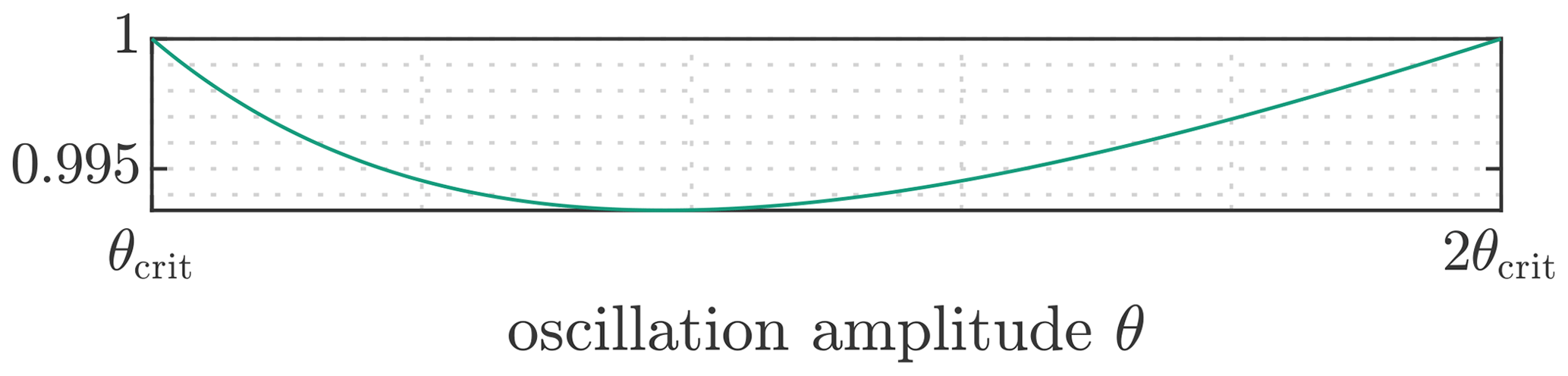
For the operational scenario shown in Fig. 4 on the right-hand side, the volume may be separated into volumes ψ₁ and ψ₂, each experiencing one or two stress cycles per half oscillation, with ${\mathit{\psi }}_{\mathrm{1}}+{\mathit{\psi }}_{\mathrm{2}}=\mathrm{360}\mathit{°}/Z$. The corresponding oscillation amplitudes are given by ${\mathit{\theta }}_{{\mathit{\psi }}_{\mathrm{1}}}+{\mathit{\theta }}_{{\mathit{\psi }}_{\mathrm{2}}}={\mathit{\theta }}_{\mathrm{crit}}$, where ${\mathit{\theta }}_{{\mathit{\psi }}_{\mathrm{2}}}=\mathit{\theta }-{\mathit{\theta }}_{\mathrm{crit}}$. Equation (A4) may then be used separately for each of the individual volumes to obtain $L_{{\mathit{\psi }}_{\mathrm{1}}}=a_{\mathrm{pr}t,{\mathit{\psi }}_{\mathrm{1}}}L$ and the overlapping volume ψ₂ experiencing twice as many cycles, giving $L_{{\mathit{\psi }}_{\mathrm{2}}}=\frac{\mathrm{1}}{\mathrm{2}}{a}_{\mathrm{prt},{\mathit{\psi }}_{\mathrm{2}}}L$. These can be combined via

$$\begin{array}{}\text{(C1)}& \begin{array}{rl}{L}_{{\mathit{\psi }}_{\mathrm{1}}+{\mathit{\psi }}_{\mathrm{2}}}& ={\left(L_{{\mathit{\psi }}_{\mathrm{1}}}^{-e}+L_{{\mathit{\psi }}_{\mathrm{2}}}^{-e}\right)}^{-\mathrm{1}/e}\\ & =\underset{a_{\mathrm{prt},{\mathit{\psi }}_{\mathrm{1}}+{\mathit{\psi }}_{\mathrm{2}}}}{\underbrace{{\left(a_{\mathrm{prt},{\mathit{\psi }}_{\mathrm{1}}}^{-e}+{\left({\displaystyle \frac{\mathrm{1}}{\mathrm{2}}}{a}_{\mathrm{prt},{\mathit{\psi }}_{\mathrm{2}}}\right)}^{-e}\right)}^{-\mathrm{1}/e}}}L.\end{array}\end{array}$$

This allows for the analysis of the Rumbarger effect for oscillations θ>θ_crit with overlapping volumes. Figure C1 shows an exemplary calculation of $a_{\mathrm{prt},{\mathit{\psi }}_{\mathrm{1}}+{\mathit{\psi }}_{\mathrm{2}}}$ for a 7220 type bearing normalized to the Harris factor. The result of $a_{\mathrm{prt},{\mathit{\psi }}_{\mathrm{1}}+{\mathit{\psi }}_{\mathrm{2}}}$ can be seen to be almost identical to a_Harris.

Figure C1 $a_{\mathrm{prt},\mathit{\alpha }+\mathit{\beta }}/a_{\mathrm{Harris}}$ for the inner ring of a 7220 type bearing for θ>θ_crit.