Evaluating the potential of short-term instrument deployment to improve distributed wind resource assessment

Distributed wind projects, which are connected at the distribution level of an electricity system or in off-grid applications to serve specific or local energy needs, often rely solely on wind resource models to establish wind speed and energy generation expectations. Historically, anemometer loan programs have provided an affordable avenue for more accurate onsite wind resource assessment, and the lowering cost of lidar systems has shown similar advantages for more recent assessments. While a full 12 months of onsite wind measurement is the standard for correcting model-based long-term wind speed estimates for utility-scale wind farms, the time and capital investment involved in gathering onsite measurements must be reconciled with the energy needs and funding opportunities that drive expedient deployment of distributed wind projects. Much literature exists to quantify the performance of correcting long-term wind speed estimates with 1 or more years of observational data, but few studies explore the impacts of correcting with months-long observational periods. This study aims to answer the question of how short you can go in terms of the observational time period needed to make impactful improvements to model-based long-term wind speed estimates.

Three algorithms, multivariable linear regression, adaptive regression splines, and regression trees, are evaluated for their skill at correcting long-term wind resource estimates from the European Centre for Medium-Range Weather Forecasts Reanalysis version 5 (ERA5) using months-long periods of observational data from 66 locations across the US. On average, correction with even 1 month of observations provides significant improvement over the baseline ERA5 wind speed estimates and produces median bias magnitudes and relative errors within 0.22 m s⁻¹ and 4 percentage points of the median bias magnitudes and relative errors achieved using the standard 12 months of data for correction. However, in cases when the shortest observational periods (1 to 2 months) used for correction are not well correlated with the overlapping ERA5 reference, the resultant long-term wind speed errors are worse than those produced using ERA5 without correction. Summer months, which are characterized by weaker relative wind speeds and standard deviations for most of the evaluation sites, tend to produce the worst results for long-term correction using months-long observations. The three tested algorithms perform similarly for long-term wind speed bias; however, regression trees perform notably worse than multivariable linear regression and adaptive regression splines in terms of correlation when using 6 months or less of observational data for correction.

Translating the analysis to wind energy, median relative errors in the capacity factor are on average within 10 % using 1 month of training. If the observation period used for correction is not well correlated with the reference data, however, misrepresentation of the observed capacity factor can be substantial. The risk associated with poor correlation between the observed and reference datasets decreases with increasing training period length. In the worst-correlation scenarios, the median capacity factor relative errors from using 1, 3, and 6 months are within 47 %, 26 %, and 16 %, respectively.

1 Introduction

In the utility-scale wind energy industry, short-term (less than 5 years) wind measurements are temporally extended using long-term (decades-long) wind resource simulations to produce a long-term wind energy generation estimate at a site of development interest in an expedient manner. Wind farm project planners install onsite wind measurement instruments (e.g., meteorological towers, lidars, sodars) to gather data but cannot wait decades to establish long-term wind resource characterization based on such measurements alone (Lackner et al., 2008). Instead, wind analysts commonly simulate the long-term wind resource by correlating the short-term onsite wind measurements with long-term reference data, such as atmospheric reanalyses, high-resolution mesoscale models, or other nearby measurements using a measure–correlate–predict (MCP) approach.

Distributed wind projects, particularly those involving small wind turbines, are more subject to challenging financial, spatial, and time constraints than utility-scale wind farms. Onsite wind measurements are often not feasible or economically viable investments, leading to many distributed wind projects that rely solely on wind resource models to establish generation estimates, which are helpful but not entirely accurate. Between 2000 and 2011, the US Department of Energy (DOE) Wind Powering America initiative sponsored an anemometer loan program to provide a more affordable avenue for onsite wind resource assessment, which resulted in the installation of 128 anemometers across the US and a template for around 20 state-administered anemometer loan programs (Jimenez, 2013). More recently, researchers from Aurora College have begun deploying mobile lidar systems in northern Canada to study the viability of wind energy in communities that are reliant on diesel, which is expensive and difficult to transport to remote locations (Seto, 2022). In the US, communities that receive DOE technical assistance to transform their energy systems, such as through the Energy Technology Initiative Partnership Project (DOE, 2025), continue to weigh the costs and benefits of onsite wind measurement. In addition to concerns regarding capital investment, communities must often reconcile the time investment involved in gathering onsite measurements with the energy needs and funding opportunities driving expedient deployment of wind turbines.

The vast majority of wind resource assessment literature supports collecting at least 1 year of onsite measurements to represent a full seasonal wind cycle, including the analyses of Dinler (2013), Liléo et al. (2013), Mifsud et al. (2018), Zakaria et al. (2018), Tang et al. (2019), and Chen et al. (2022). Miguel et al. (2019) found that uncertainty in long-term wind resource estimates reduced by 18 %, 29 %, 35 %, and 40 % when 1, 2, 3, and 4 years of wind measurements, respectively, were added to the monitoring campaign. Additionally, private companies that specialize in providing resource assessment for wind projects also tend to require at least 1 year of onsite measurements to characterize the wind. For example, ArcVera uses at least 1 full year of observational data to bias correct their high-resolution model output (ArcVera, 2023). In their discussion of wind resource assessment, the wind measurement company NRG Systems (2023) states that measurements of meteorological parameters are typically taken over the course of several years at a potential wind farm site using a combination of meteorological towers and lidars.

A small number of studies, however, explore adjusting long-term predictions using observational data with less than 1 year of temporal coverage. Taylor et al. (2004) (as reported via Carta et al., 2013), Weekes and Tomlin (2014), and Basse et al. (2021) reported that wind speed errors were within 4 %, 4.8 %, and 4 %, respectively, using 3 months of onsite measurements. Using data from the United Kingdom, Derrick (1992) (as reported via Rogers et al., 2005) found that 8 months of onsite data was needed to minimize uncertainties. The performance of long-term predictions using less than 1 year of on-site measurements varied according to the season(s) during which the onsite measurements were taken. For their experiment in the United Kingdom, Weekes and Tomlin (2014) found that the smallest errors occurred when using measurements taken in early spring or fall. Basse et al. (2021) performed MCP tests in Germany using linear regression and variance ratio algorithms and found that using variance ratio produced overestimates when using summer measurements and underestimations when using winter measurements, with the opposite trend noted for linear regression.

The present study expands previous analyses of long-term wind resource performance based on months-long observations to diverse locations across the US, with a focus on measurement heights relevant to distributed wind installations (20–100 m). We explore multiple MCP algorithm options and highlight the best performers for generating accurate long-term wind speed estimates for a variety of error metrics relevant to the wind energy industry. Section 2 describes the wind measurements employed as (1) the months-long training input for MCP-based long-term wind estimates and (2) the long-term datasets to validate the MCP results. The reference dataset, the European Centre for Medium-Range Weather Forecasts Reanalysis version 5 (ERA5), is also discussed in Sect. 2, along with three MCP algorithms selected for evaluation and the error metrics employed to test their performance. Section 3 provides the performance analysis of MCP-based long-term wind resource estimation with less than 1 year of onsite measurements, with a focus on establishing the minimum number of months needed for certain levels of accuracy. Additionally, Sect. 3 relates the performance results to a variety of influences, including geographical location and the time of year that measurements were gathered. Section 4 summarizes the performance analysis and relates the wind speed error metrics to impacts on wind energy generation expectations.

2 Data discussion and methodology

The MCP model for long-term wind resource assessment begins with establishing a short-term relationship between observational wind data measured at a target site and concurrent data at a nearby reference site. The reference data can be observations or model data and typically include wind variables (speed and direction) and potentially additional relevant meteorological (temperature, pressure) or temporal (hour of day, month of year) variables. The resultant short-term relationship is subsequently applied to long-term data from the reference site to predict the long-term wind resource at the target site (Rogers et al., 2005).

2.1 Wind observations

The 66 wind speed observational datasets in this analysis are sourced from US Department of Energy national laboratories, facilities, and projects; the National Data Buoy Center; the Bonneville Power Administration; and the Forest Ecosystem Monitoring Cooperative. One observational dataset was collected using a lidar, and the remaining measurements were gathered from anemometers on meteorological towers. Most of the observational collection is publicly available (57 sites), while a small number of datasets are subject to non-disclosure agreements (9 sites), as outlined in the “Data availability” statement.

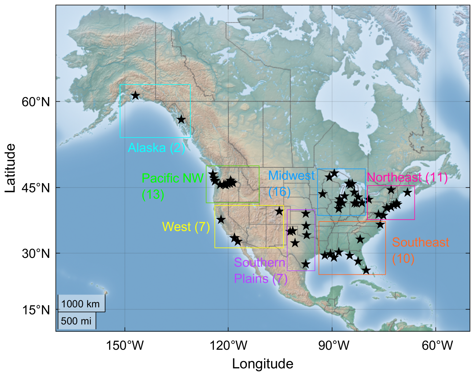
Figure 1 Locations of wind measurements assessed for establishing long-term performance based on months-long observations used in this study. The number of observational sites per region is included in parentheses.

The measurement sites utilized in this work span 28 states and are diverse in terrain complexity and land cover (Fig. 1). The measurement heights are similarly diverse, from 20 to 100 m (Fig. 2a), representing a wide range of the distributed wind hub heights that are reported in the US (PNNL, 2024). Many of the lowest observations, which align with small distributed wind turbine hub heights (between 20 and 40 m), are sourced from the National Data Buoy Center and are located along coastlines. The highest observations, which align with large distributed wind turbine hub heights (between 80 and 100 m), are in Long Island, New York (85 m), and the San Francisco Bay Area, California (100 m).

To establish reliable datasets for MCP training and validation, the wind speed observations were quality controlled by removing instances or periods of atypical or unphysical reported wind speeds (less than 0 m s⁻¹, greater than 50 m s⁻¹, or nonvarying periods of time greater than 4 hours) that might indicate instrument error due to an outage or weather impacts such as icing. The temporal coverage of the wind speed observations at the measurement sites ranged from 3.5–23 years, with an average of 11 years (Fig. 2b). The long-term measurement wind speeds ranged from 2.0 to 9.1 m s⁻¹ with an average across all measurement sites of 5.6 m s⁻¹.

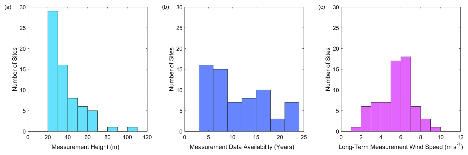
Figure 2 (a) Measurement heights, (b) long-term measurement availability, and (c) long-term measurement wind speeds for the sites evaluated for long-term performance based on months-long observations.

2.2 Reanalysis model for long-term correction

ERA5 is a popular global reanalysis model (Hersbach et al., 2020) utilized for wind energy resource assessments in a variety of ways, including as a standalone product, as input boundary conditions to higher-resolution model runs, and as a reference dataset for MCP with local observations (Olauson, 2018; Soares et al., 2020; Hayes et al., 2021; de Assis Tavares et al., 2022). ERA5 was developed by the European Centre for Medium-Range Weather Forecasts and provides meteorological data from 1950–present at 1 h temporal resolution with a horizontal grid spacing of 0.25° (Hersbach et al., 2020). At many locations where validation has been performed, ERA5 tends to produce high Pearson correlation coefficients (Eq. 1) and negative biases (indicating underestimation) (Eq. 2) between the simulated (u_sim) and observed (u_obs) wind speeds. Ramon et al. (2019) utilized 77 meteorological towers around the globe with measurement heights ranging from 10 to 122 m and found median ERA5 seasonal wind speed biases between 0 and −1 m s⁻¹, though ERA5 had the best correlation with observations among five reanalyses. Across 62 sites in the continental US, Sheridan et al. (2022) found that ERA5 underestimated the observed wind speeds by an average of 0.5 m s⁻¹ but had higher correlations (average of 0.77) than two alternate reanalyses and wind models. Using measurements from more than 100 onshore and offshore lidars, sodars, and meteorological towers across the US, Wilczak et al. (2024) determined that ERA5-derived wind power estimates were biased low by 20 %. At locations across Europe, Murcia et al. (2022) determined that ERA5 slightly underestimated the observed wind speeds (average bias of −0.06 m s⁻¹) and provided a high degree of correlation (average of 0.92).

2.3 Metrics for performance evaluation

This study aims to reduce the ERA5-based wind speed bias using months-long onsite observations while not degrading other metrics of error, such as correlation. The Pearson correlation coefficient explains the degree to which the simulated and observed wind speeds are linearly related, with values close to 1 indicating a high degree of correlation (Eq. 1). The wind speed bias, i.e., the average difference between the simulated (U_sim) and observed (U_obs) wind speeds over a time series of length N, indicates whether a simulation tends to overestimate (positive bias), underestimate (negative bias), or accurately represent (zero bias) the observed wind resource (Eq. 2). This work also considers the bias magnitude (the absolute value of bias (Eq. 2)) when comparing multiple sites, as combinations of positive and negative biases can obscure the degree of error. The relative error in the long-term wind speed simulation is the absolute difference between the simulated and observed wind speeds normalized by the observed wind speed, providing insight into the magnitude of error in a simulation (Eq. 3).

$$\begin{array}{}\text{(1)}& {\displaystyle }\mathrm{correlation}={\displaystyle \frac{{\sum }_{i=\mathrm{1}}^N\left(U_{\mathrm{sim},i}-\stackrel{\mathrm{‾}}{U_{\mathrm{sim}}}\right)\left(U_{\mathrm{obs},i}-\stackrel{\mathrm{‾}}{U_{\mathrm{obs}}}\right)}{\sqrt{{\sum }_{i=\mathrm{1}}^N{\left(U_{\mathrm{sim},i}-\stackrel{\mathrm{‾}}{U_{\mathrm{sim}}}\right)}^{\mathrm{2}}\sqrt{{\sum }_{i=\mathrm{1}}^N{\left(U_{\mathrm{obs},i}-\stackrel{\mathrm{‾}}{U_{\mathrm{obs}}}\right)}^{\mathrm{2}}}}}}\text{(2)}& {\displaystyle }\mathrm{bias}={\displaystyle \frac{\mathrm{1}}{N}}\sum _{i=\mathrm{1}}^N\left(U_{\mathrm{sim},i}-U_{\mathrm{obs},i}\right)\text{(3)}& {\displaystyle }\text{relative error}=\mathrm{100}\mathit{\%}\times {\displaystyle \frac{⌈\stackrel{\mathrm{‾}}{U_{\mathrm{sim}}}-\stackrel{\mathrm{‾}}{U_{\mathrm{obs}}}⌉}{\stackrel{\mathrm{‾}}{U_{\mathrm{obs}}}}}\end{array}$$

To set a baseline of ERA5 performance for the suite of observations utilized in this work, we adjust the ERA5 wind speeds to each measurement height z (Fig. 2a) using the power law (Eq. 4) with the shear exponent α calculated at each timestamp using ERA5 wind speeds at 10 and 100 m (Eq. 5). Horizontally, we adjust the ERA5 wind speeds to the observational location using inverse distance-weighted interpolation.

$$\begin{array}{}\text{(4)}& {\displaystyle }{U}_{\text{era5\_z}}=U_{\text{era5\_100m}}{\left({\displaystyle \frac{z}{\mathrm{100}\mathrm{m}}}\right)}^{\mathit{\alpha }}\text{(5)}& {\displaystyle }\mathit{\alpha }={\displaystyle \frac{\ln \left(U_{\text{era5\_100m}}/U_{\text{era5\_10m}}\right)}{\ln \left(\mathrm{100}\mathrm{m}/\mathrm{10}\mathrm{m}\right)}}\end{array}$$

In all regions except for the southeast, the ERA5 wind speeds tend to be lower than the observed wind speeds (Fig. 3a). The underestimation is most pronounced in Alaska (median bias of −1.61 m s⁻¹), the Pacific Northwest (−1.18 m s⁻¹), and the Southern Plains (−1.74 m s⁻¹). The same three regions have the highest relative errors (medians of 28 %, 25 %, and 20 %, respectively) (Fig. 3b). The median correlations exceed 0.75 for all regions except Alaska (0.69) and the west (0.67), where the coarse ERA5 is challenged by mountainous and coastal terrain (Fig. 3c). No consistent trends in ERA5's performance are noted according to height above ground (Fig. 3d, e, f). The wind speed relative errors are the greatest for measurement heights between 30 and 40 m (median of 31 %), while the median relative errors for measurement heights between (1) 20 and 30 m and (2) 40 and 50 m are 11 % and 10 %, respectively. Across all sites, the median statistics are as follows: a bias of −0.50 m s⁻¹, bias magnitude of 0.67 m s⁻¹, relative error of 13 %, and correlation of 0.78. The tendency of ERA5 to underestimate the observed wind speeds in this analysis while exhibiting a relatively high degree of correlation with them aligns with the findings of Ramon et al. (2019), Murcia et al. (2022), Sheridan et al. (2022), and Wilczak et al. (2024) discussed in Sect. 2.2. The bias trends according to region (Fig. 3a) also align with the findings of Wilczak et al. (2024) in that ERA5 underestimation is noted in the Pacific Northwest and Southern Plains, while a mix of overestimation and underestimation is noted for the Midwest.

Figure 3 Long-term ERA5 wind speed bias (a, d), relative error (b, e), and correlation (c, f) across 66 measurement sites in the US, grouped by region (a–c) and measurement height (d–f). AK – Alaska, PNW – Pacific Northwest, W – west, MW – Midwest, SP – Southern Plains, NE – northeast, and SE – southeast.

2.4 MCP methodologies

One of the advantages of utilizing MCP for long-term wind resource estimation is the variety of algorithm choices, which range from simplistic linear regression to machine learning techniques that can be applied to link short-term and long-term wind speeds. Early MCP methodologies focused on linear (as reported via Rogers et al., 2005: Derrick, 1992; Landberg and Mortenson, 1994; Woods and Watson, 1997; Vermeulen et al., 2001) and quadratic fits (as reported via Rogers et al., 2005: Joenson et al., 1999; Riedel and Strack, 2001). From there, distribution-based probabilistic techniques emerged (García-Rojo, 2004; Sheppard, 2009; Carta and Velázquez, 2011). With the onset of machine learning techniques came applications to MCP-based wind resource analysis, such as using artificial neural networks, support vector machines, and random forest to estimate long-term wind speeds (Díaz et al., 2018).

This analysis evaluates three algorithms for their skill at creating long-term wind resource estimates based on varying temporal lengths of observational data: (1) multiple linear regression (MLR), (2) adaptive regression splines (ARSs), and (3) regression trees (RTs). These algorithms were selected because they are broadly available and represent diversity in complexity and approach. Multiple linear regression estimates the linear relationship between a target variable (onsite wind measurements in this analysis) and more than one reference variable (sourced from ERA5 in this analysis). Adaptive regression splines involve the construction of piecewise-cubic regression models based on the short-term target and reference datasets (Jekabsons, 2016). In this analysis, we utilize the default parameter configurations of Jekabsons (2016). The maximum number of basis functions follows the formula of Milborrow (2016): min(200, max(20, 2 × the number of input variables)) + 1. The maximum degree of interactions between input variables is set to 1 for additive modeling; therefore the generalized cross-validation penalty per knot is set to 2 following the recommendation of Friedman (1991). Regression trees recursively evaluate the concurrent short-term target and reference datasets and partition them into unique segments, which are subsequently used to predict long-term target behavior. In this analysis, the ensemble aggregation method used is least-squares boosting with 100 learning cycles, as per the MATLAB algorithm fitrensemble (MathWorks, 2024). Numerous additional algorithms have been developed and tested for their ability to improve simulation accuracy, and it is important to note that each features different approaches, computational investments, complexities, skills, and limitations. For example, Rogers et al. (2005) note that linear regression techniques are easily implemented and well suited for performing bias correction but have a tendency to create a bias in the variance that variance-conserving MCP techniques are better suited to resolve.

To narrow down an effective training approach, different combinations of reference variables are explored for their impact on long-term wind resource assessment error metrics. The analysis of Phillips et al. (2022) identified reanalysis wind speed, reanalysis wind direction, and time of day as the most important variables for wind speed bias correction using a variety of techniques, including multivariable linear regressions and regression trees. Therefore, we explore progressively increasing variable combinations of ERA5 wind speeds at the provided output heights of 10 and 100 m (U_{era5_10m} and U_{era5_100m}), power-law-based wind speed estimates at the measurement height z (U_{era5_z}) (Eq. 4) using the shear exponent α based on ERA5 wind speeds at 10 and 100 m (Eq. 5), ERA5 u and v wind components at 10 and 100 m (u_{era5_10m}, v_{era5_10m}, u_{era5_100m}, and v_{era5_100m}), and the hour of the day.

As an initial test of the performance of the algorithms and reference variable combinations, we develop ensembles of MCP-based long-term wind speed estimates at each measurement site using consecutive 12-month training periods, according to the following steps:

1. We establish that 75 % of the observations in each month in the training period are available after applying the quality-control checks discussed in Sect. 2.1 (all 66 observations utilized in this work have average and median monthly data recovery and quality rates exceeding the 75 % threshold).

2. A model is trained on temporally aligned observation data and reference data during the training period.

3. The model is used to predict the full observation period (Fig. 2b).

4. Performance statistics are computed with respect to the observations (Table 1). Timestamps with missing observations are excluded from the statistics.

Table 1 Long-term MCP-based wind speed error metrics averaged (median) across 66 sites using different combinations of algorithms and training variables. Values in bold indicate the optimal combination of training variables for each error metric and algorithm.

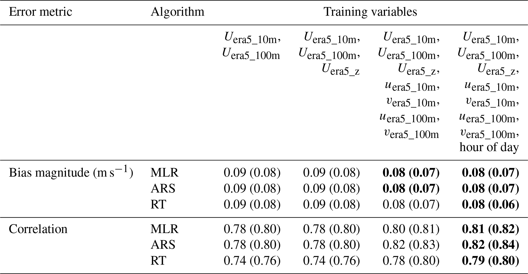
All MCP combinations of algorithms and training variables provide substantially improved long-term bias magnitudes compared to the ERA5 (i.e., U_{era5_z}) average (median) bias magnitude of 1.01 m s⁻¹ (0.67 m s⁻¹) (Table 1). With 12 months of training time, the MCP average and median bias magnitudes vary by at most 0.02 m s⁻¹ according to algorithm and training variables. More variability is seen according to the various combinations of MCP algorithms and training variables for correlation (Table 1). Using just U_{era5_10m} and U_{era5_100m} as training variables, MLR and ARS improve on the ERA5 average (median) correlation of 0.76 (0.77), while RT produces a lower correlation. Utilizing all training variables generates the highest overall correlations (Table 1). Given the optimal correlation results found when training for 12 months with MCP using the complete variable set of ERA5 wind speeds, ERA5 u and v components, and hour of the day, these variables are selected for evaluating long-term MCP wind speed estimates using months-long training periods. Using 12 months of observations, the three algorithms perform similarly for bias, and ARS is the best-performing algorithm for correlation. The following sections explore whether that status holds when using months-long training periods.

The months-long analysis follows the same ensemble formula as the 12-month exercise, just with shorter consecutive training periods. Across the measurement sites, calendar months in the spring and fall had the most single instances of ≥75 % data recovery and quality, followed by summer and, lastly, winter (Fig. 4). Median measurement data recovery and quality percentages according to calendar month ranged from 99.2 % (December) to 99.7 % (May) (Fig. 4).

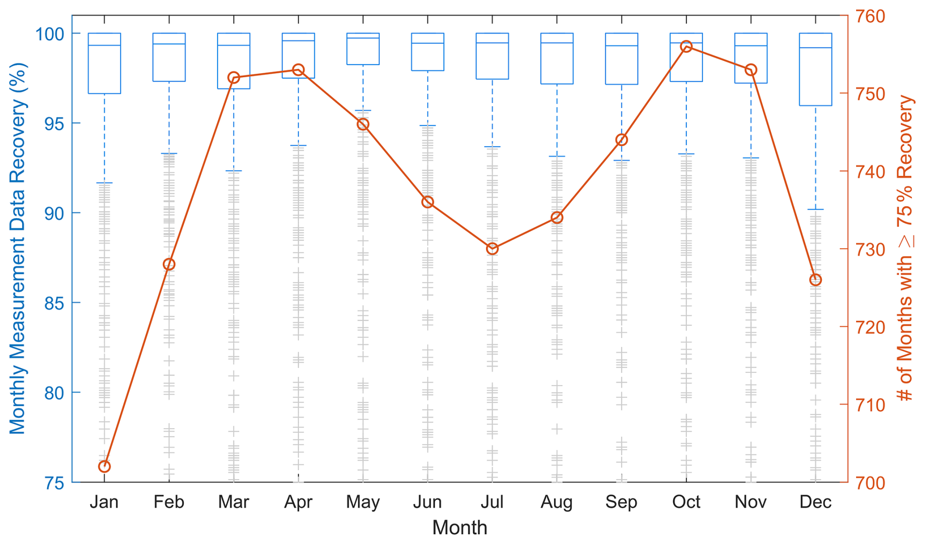
Figure 4 Monthly measurement data recovery and quality (boxplot) and number of months with ≥75 % data recovery.

3 Results and discussion

3.1 Long-term wind estimation performance according to length of training period

On average, even 1 month of observations combined with any of the three assessed MCP algorithms provides substantial improvement over using ERA5 wind speeds alone for long-term wind speed estimation. Figure 5a displays the ensemble average bias magnitude at each site using increasing numbers of training months. The median bias magnitudes across all sites using 1 month of training are 0.28 m s⁻¹ (MLR) and 0.29 m s⁻¹ (ARS, RT), as compared with 0.67 m s⁻¹ using ERA5 (Table 2, Fig. 5a). The median bias magnitudes drop to 0.18 m s⁻¹ using 3 months of training and 0.12 m s⁻¹ using 6 months of training. For all training durations, the MCP algorithms perform within 0.01 m s⁻¹ of each other for median bias magnitude. Similarly, the relative errors in the long-term wind speed estimates decrease substantially from those using ERA5 (median 13 %) (Fig. 5b). A total of 1 month of training produces median relative errors of 6 % across the algorithms, which decreases to 4 % with 3 months of training and 2 %–3 % with 6 months of training (Table 2). The standard deviations of bias magnitude provide an indication of the uncertainty in the MCP-based long-term wind speed estimates, ranging from 0.24 m s⁻¹ (MLR, RT) to 0.28 m s⁻¹ (ARS) using 1 month of training, 0.14 m s⁻¹ (RT) to 0.15 m s⁻¹ (MLR, ARS) using 3 months of training, and 0.08 m s⁻¹ (ARS, RT) to 0.09 m s⁻¹ (MLR) using 6 months of training (Fig. 5c, Table 2).

Table 2 Median biases, bias magnitudes, standard deviations of bias magnitudes, relative errors, and correlations according to algorithm and number of training months.

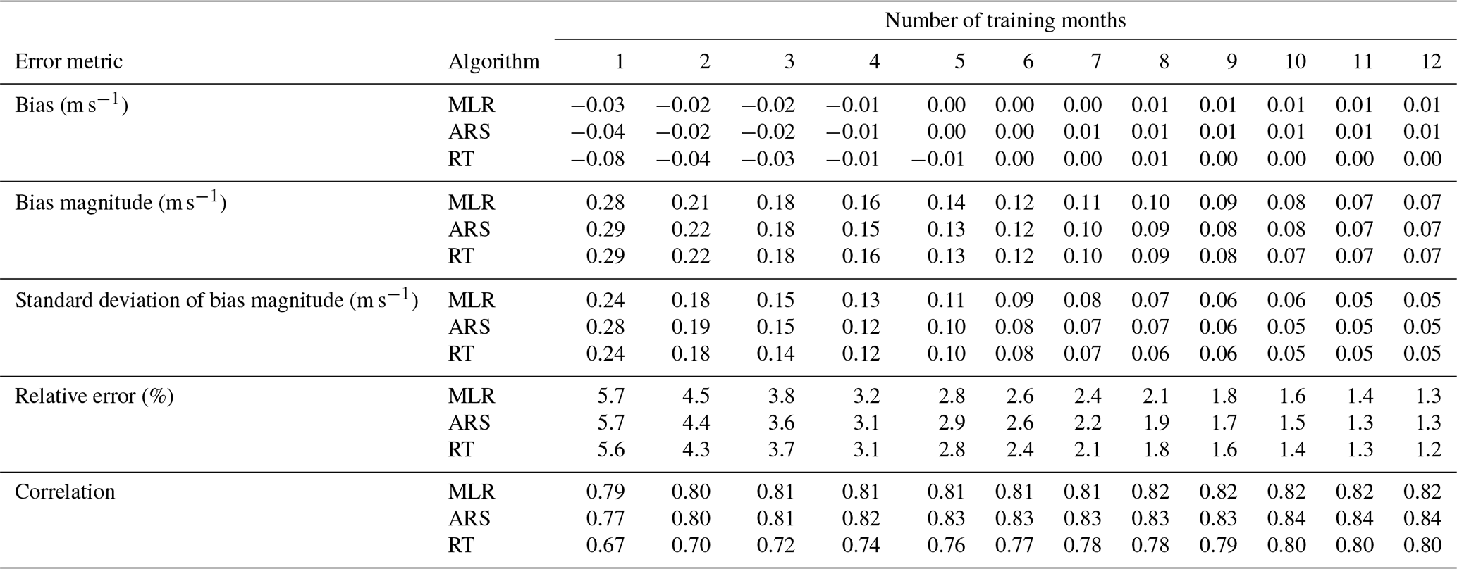
Considering the sign of the bias, we recall that ERA5 tends to underestimate the observed wind speeds with a median bias of −0.50 m s⁻¹ across the sites. On average, incorporating months-long observations into the long-term estimations moves the bias substantially closer to zero. Applying just 1 month of observations results in median biases between −0.08 m s⁻¹ (RT) and −0.03 m s⁻¹ (MLR). For all training period lengths of 4 months or greater, the median MCP-based biases are within ±0.01 m s⁻¹, regardless of algorithm (Table 2).

The MCP algorithms diverge in their performance for long-term wind speed correlation, especially when using 4 or fewer training months. Using RT with a limited number of training months does not improve correlation relative to ERA5 and the other MCP algorithms. Using 1 month of training, MLR and ARS produce similar correlations (medians of 0.79 and 0.77, respectively) to ERA5 (median of 0.78), while the RT correlations are markedly worse (median of 0.67) (Table 2, Fig. 5d). Only when the training period is at least 7 months do the median RT correlations match ERA5. An interesting correlation comparison is noted for the National Renewable Energy Laboratory's National Wind Technology Center, located in an extremely windy corridor of the complex terrain along Colorado's Front Range. All of the lowest correlation outliers in Fig. 5d are from this site, and, while MLR and ARS match or improve upon the ERA5 correlation for the National Wind Technology Center (0.47) using any training period length of at least 2 months, RT never achieves the ERA5 correlation, even with a full 12 months of training. For all training durations of at least 4 months, ARS is on average the best-performing MCP algorithm for correlation.

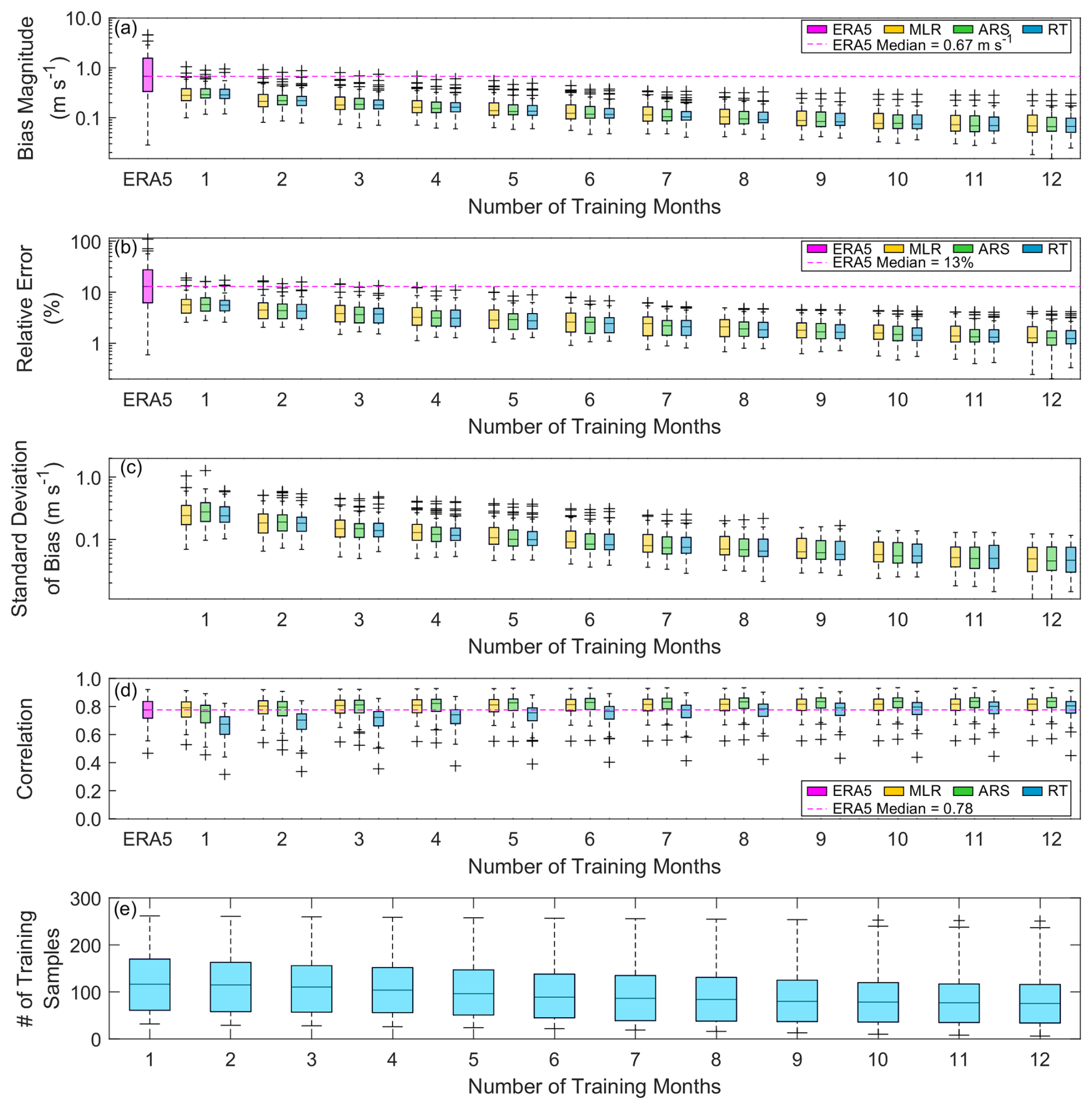
Figure 5 Average long-term (a) bias magnitude, (b) relative error, (c) standard deviation of bias magnitude, and (d) correlation for 66 sites comparing observations with ERA5 and MCP techniques using varying training period lengths, along with (e) the number of training samples per site and per number of training months.

Given that a 12-month training period is most commonly employed for long-term wind speed estimation using MCP, it is beneficial to consider MCP performance using less than 1 year of observations relative to the 12-month standard. Using a 1-month training period, the median long-term bias magnitudes (relative errors) for 66 sites are within 0.22 m s⁻¹ (4 percentage points) of the median long-term bias magnitudes (relative errors) determined using 12 months, regardless of the MCP algorithm (Fig. 6a, b). However, at one coastal Alaskan site, the difference in bias magnitude (relative error) when using 1 versus 12 months of observations can reach 1 m s⁻¹ (18 %). Training with 3 months of observations places the median bias magnitudes (relative errors) within 0.12 m s⁻¹ (3 percentage points) of the median bias magnitudes (relative errors) established when using 12 months, with outlier differences within 0.7 m s⁻¹ (13 %). Using 6-month training periods results in median bias magnitudes (relative errors) within 0.05 m s⁻¹ (1 percentage point) of the 12-month median bias magnitudes (relative errors), with outlier differences within 0.4 m s⁻¹ (6 %).

A great disparity is noted among the MCP algorithms when comparing their correlation performance using months-long training periods versus training periods of a 1-year duration (Fig. 6c). Using 1 month of training versus 12 months produces median correlation differences of 0.03 for MLR, 0.07 for ARS, and 0.13 for RT. With 6-month training periods, MLR and ARS produce a median correlation that differs by less than 0.01 from that using 12 months, while the 6-month median RT correlation differs by 0.04 compared to that using 12 months.

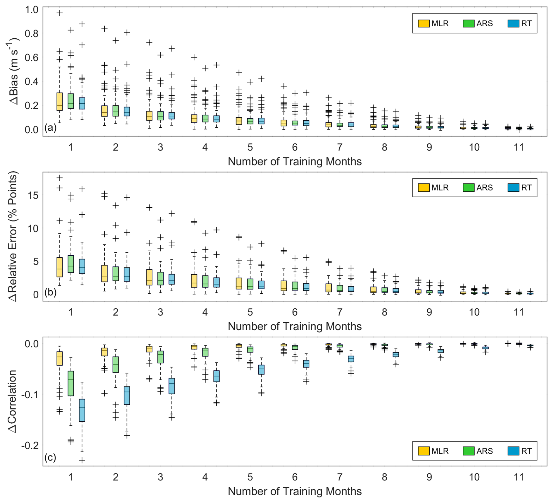
Figure 6 Difference in average long-term (a) bias magnitude, (b) relative error, and (c) correlation for 66 sites between MCP training periods of 1 to 11 months and MCP training periods of 12 months.

The results in Figs. 5 and 6 explain the degree of error expected on average when using MCP with observations less than 1 year in duration, highlighting similar performance across the MCP algorithms for long-term wind speed bias magnitude but less successful performance when using RT with months-long observations for correlation. However, since wind measurement timelines tend to be more dependent on funding availability, project deadlines, and fair-weather deployment windows than on identifying the most representative period for long-term wind representation, it is imperative to consider the worst-case-scenario errors (Fig. 7). In this scenario, we identify the worst-performing ensemble member for each error metric (largest bias magnitude, largest MAE, smallest correlation) and each algorithm (MLR, ARS, RT) according to the length of the training period for each of the 66 sites. It is important to keep in mind that the worst-case-scenario error analysis is a conservative approach that is not analogous to assessing algorithm uncertainty. Additionally, more robust algorithms than those studied in this work could reduce the sensitivity to the outliers in the shortest training time series that drive errors in the long-term estimates.

In the worst-case scenario, using a single month for MCP training will produce long-term errors that are significantly worse than those simply using ERA5 to produce long-term wind speed estimates (Fig. 7). Despite its performance success on average (Fig. 5), ARS produces the largest bias magnitudes (median of 1.36 m s⁻¹), the largest relative errors (median of 27 %), and the smallest correlations (median of 0.20) in the worst-case scenario. MLR and RT perform similarly for bias using a 1-month training period in the worst-case scenario (median bias magnitudes of 1.23 m s⁻¹ and 1.18 m s⁻¹, respectively; median relative errors of 22 % for both algorithms), while MLR performs best in terms of correlation (median of 0.63).

A training period of 4 months provides improvement in bias magnitude and relative error over simply using ERA5 (medians of 0.67 m s⁻¹ and 13 %, respectively) for long-term wind resource estimation, even in the worst-case scenario, regardless of MCP algorithm choice (medians of 0.53–0.59 m s⁻¹ and 13 %, respectively) (Fig. 7). For correlation, MLR exceeds ERA5 (median of 0.78) at 5 months, ARS at 6 months, and RT at 12 months (medians of 0.79). Although all three algorithms provide similar improvement in relative errors and MLR and ARS provide the most beneficial correlations on average when using MCP with months-long observations (Fig. 5, Table 2), MLR is the least risky approach given the possibility of measurement during unfavorable wind conditions for MCP.

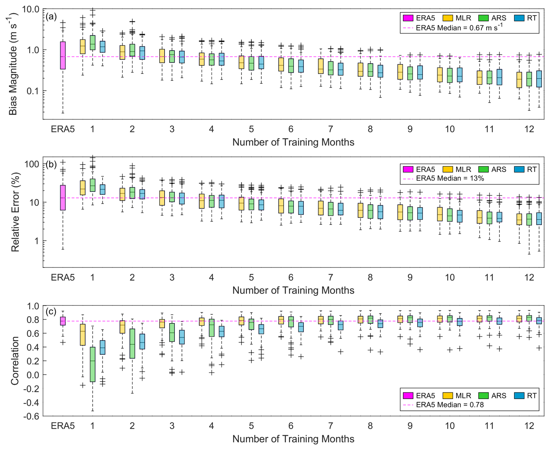
Figure 7 Worst-case long-term (a) bias magnitude, (b) relative error, and (c) correlation for 66 sites comparing observations with ERA5 and MCP techniques using varying training period lengths.

To help us understand what the unfavorable conditions are that might lead to a worst-case scenario, we investigate the characteristics of the wind speed observations during the worst-case-scenario periods relative to the average characteristics of the wind speed observations across all training periods with the same duration (Fig. 8). It is interesting to note that the dates of the training time periods with the worst-case scenarios are variable according to the MCP algorithm and error metric, particularly for the shortest-duration training periods. We find that both the mean and the standard deviation of the observed wind speeds during the worst-case-scenario month or consecutive months tend to be lower than the mean and standard deviation of the observed wind speeds across all periods with the same durations, particularly when using ARS and RT (Fig. 8). In other words, low-wind-speed time periods with correspondingly low variations in wind speeds tend to provide the biggest challenges for long-term MCP accuracy. For example, the median observed wind speed mean (standard deviation) across the 66 sites for all 1-month-duration periods is 5.80 m s⁻¹ (3.12 m s⁻¹), while the 1-month worst-case scenario for ARS based on relative error corresponds to an observed wind speed mean (standard deviation) of 4.61 m s⁻¹ (2.30 m s⁻¹) (Fig. 8a, b). Increasing numbers of training months correspond with higher mean wind speeds and standard deviations during the worst-case periods, along with convergence of the worst-case-scenario mean wind speeds and standard deviations to mean wind speeds and standard deviations across all training periods of the same durations.

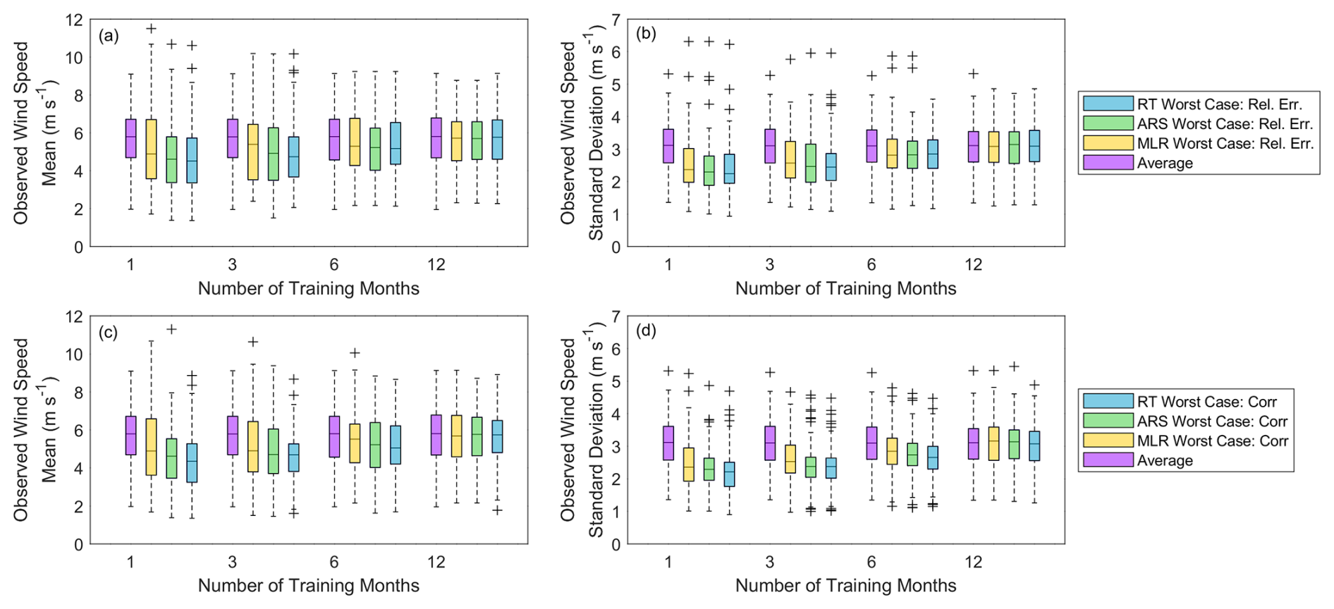
Figure 8 (a, c) Mean wind speed and (b, d) wind speed standard deviation across 66 sites for MLR, ARS, and RT worst-case scenarios for (a, b) relative error and (c, d) correlation and across all training periods for each site of the same durations. Only the results using 1, 3, 6, and 12 months of training are presented for the sake of brevity. Increasing numbers of training months correspond with convergence of the worst-case-scenario mean wind speeds and standard deviations to mean wind speeds and standard deviations across all training periods of the same duration.

3.2 Regional long-term wind estimation performance

On average, using 1 month of observations produces regional median relative errors within 8 % using any of the three MCP algorithms, except for the two Alaskan sites (Fig. 9a–g). The Alaskan median relative errors are substantially higher (16 % using MLR, 14 % using ARS, and 15 % using RT) but still significantly lower than the ERA5 median relative error for these two sites (28 %) (Fig. 3a). The most impressive reduction in bias magnitude occurs for the Southern Plains, where ERA5 produces a median relative error of 20 % (Fig. 3a) that decreases to 3 % (MLR) or 4 % (ARS, RT) with the addition of just 1 month of observations (Fig. 9e). Using 3 and 6 months of observations, all median regional relative errors are within 5 % and 4 %, respectively, except for Alaska, where the median relative errors range from 11 % (ARS, RT) to 12 % (MLR) using 3 months of observations and 6 % (ARS, RT) to 7 % (MLR) using 6 months of observations. Using 12 months of observations, all regional bias magnitudes are within 3 %, including Alaska (Fig. 9a–g). A potential factor impacting the results for Alaska is the quality of the observations. While the automated quality-control techniques discussed in Sect. 2.1 remove periods of nonvarying wind speeds due to outages or icing, they may not capture more subtle impacts on the observations, such as partial icing of the anemometers.

On average, using RT with 1 month of observations degrades the ERA5 median correlations in all regions. Considering all sites, MLR tends to improve on the ERA5 correlations using 1 month of observations, while ARS performs similarly to ERA5 (Fig. 5d). However, when exploring correlation on a regional scale, MLR performs similarly to ERA5 using 1 month of observations in all regions except the west, while ARS performs similarly to ERA5 in the Pacific Northwest, Midwest, and northeast and worsens relative to ERA5 in all other regions (Fig. 9h–n).

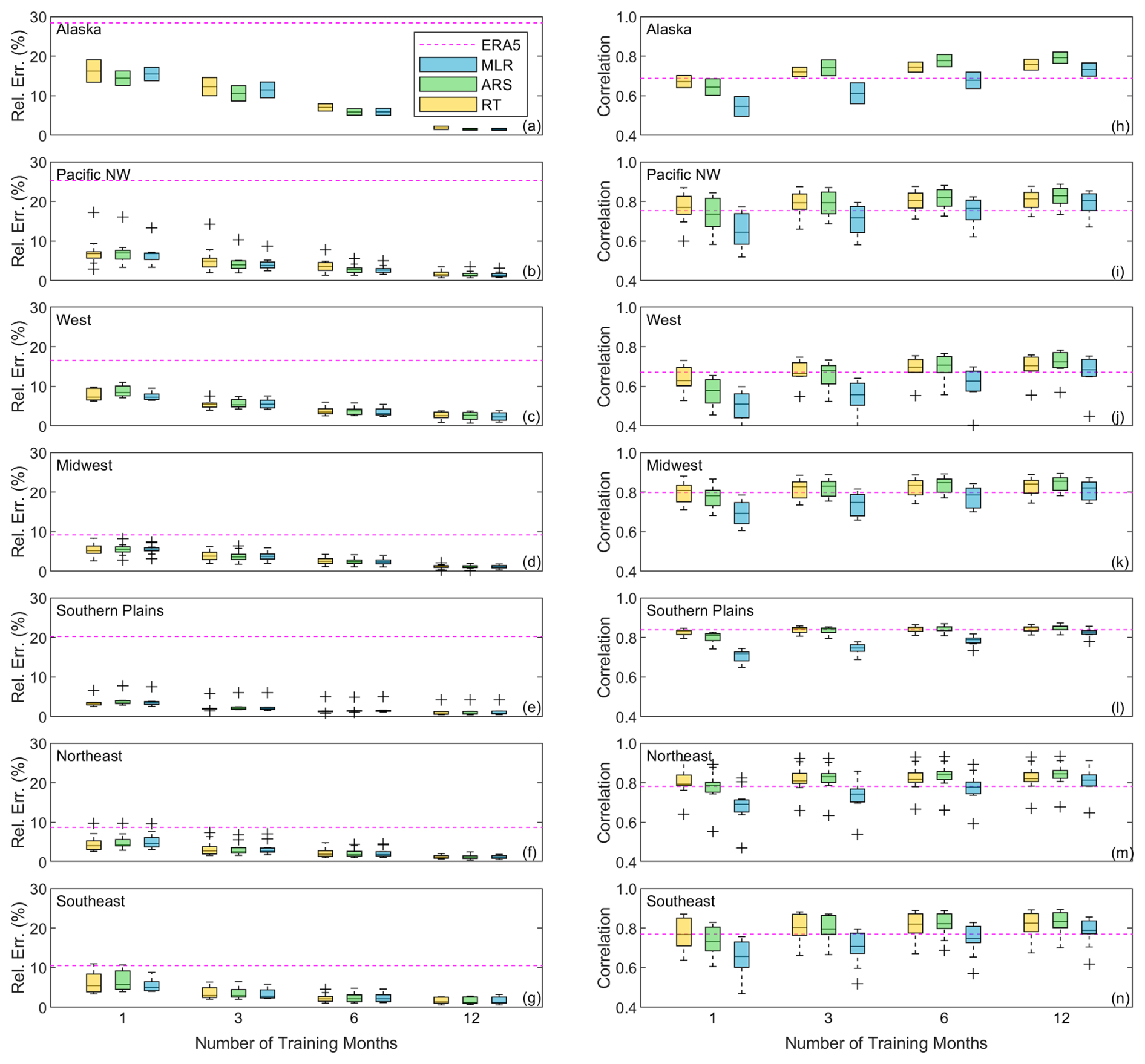
Figure 9 Long-term wind speed relative error (left) and correlation (right) according to region for varying training period lengths.

3.3 Seasonal relationships between observations and long-term wind estimation performance

When considering using less than 1 year of wind speed measurements to correct long-term wind speed estimates, it is important to select the most optimal time of year to gather such measurements (and to understand what times of year to avoid). For each of the 66 sites, Figs. 10 and 11 share the best and worst single months, on average, for optimizing error metrics when applying MCP to ERA5. The best months for optimizing relative error using all three MCP algorithms are quite variable across non-summer (June, July, August) months, with winter (December, January, February), spring (March, April, May), and fall (September, October, November) producing the most optimal relative errors at 21 %–23 %, 35 %–41 %, and 30 %–33 % of the 66 sites, respectively (Fig. 10). For correlation, spring months produce the best results when using MLR and ARS for 55 % and 48 % of the sites, respectively. When using RT, fall months produce the best correlations at 41 % of the sites. Summer months, particularly July and August, tend to produce the worst relative errors and correlations (Fig. 11) and should be avoided if opting to create MCP-based wind speed estimates using a single season of observations. July and August produce the highest relative errors at 52 %–56 % of the 66 sites, depending on the selected algorithm, and the lowest correlations at 61 %–73 % of the sites.

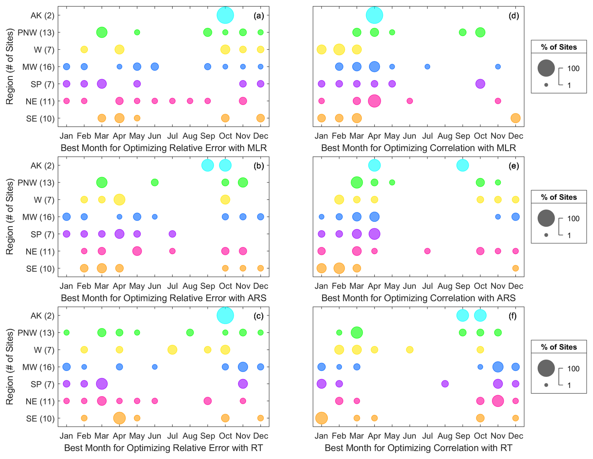
Figure 10 Best average single months for optimizing (a, b, c) relative error and (d, e, f) correlation when creating MCP-based long-term wind speed estimates using (a, d) MLR, (b, e) ARS, and (c, f) RT according to each US region. Larger circles indicate the best month for more sites in a given region.

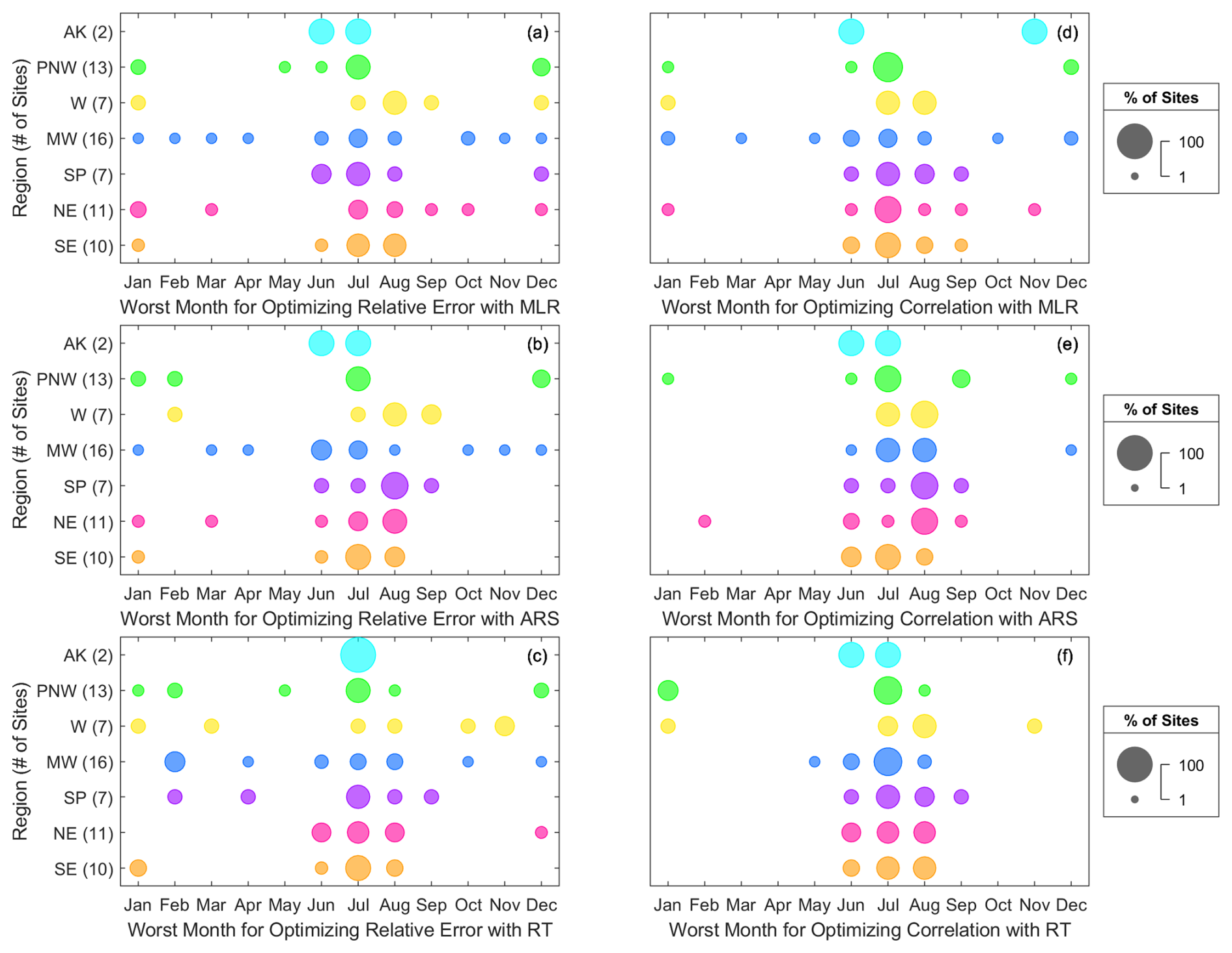
Figure 11 Worst average single months for optimizing (a, b, c) relative error and (d, e, f) correlation when creating MCP-based long-term wind speed estimates using (a, d) MLR, (b, e) ARS, and (c, f) RT according to each US region. Larger circles indicate the best month for more sites in a given region.

3.4 Implications for energy production estimates

On average, utilizing months-long observations to correct reanalysis-based long-term wind speed estimates provides significant improvement in accuracy of predicted winds (Fig. 5). However, substantial risks to accuracy occur when the months-long observational period misrepresents longer-term wind speed trends (Fig. 7). To evaluate the impacts of long-term correction using months-long observations on distributed wind energy production, we convert the long-term observed and simulated wind speeds to energy estimates using the National Renewable Energy Laboratory's 100 kW distributed wind reference power curve (NREL, 2019). Since variable lengths of long-term periods are utilized in this study, we opt to consider energy production in terms of the capacity factor, i.e., the energy estimate divided by the product of the total number of hours in the long-term period and the turbine rated capacity (100 kW in this example). The observed wind speeds in this analysis produce gross (i.e., no loss considered) capacity factors ranging from 3 % (inland Louisiana) to 66 % (Texas panhandle), with an average (median) of 34 % (36 %). The low wind speeds at some of these sites are not suitable for wind energy deployment. Additionally, the power production at the low-wind-speed sites will be dominated by the tail end of the wind speed distribution, leading to potentially significant differences between the skill of the MCP algorithms in reproducing the highest percentiles of wind speeds versus estimating mean wind speeds, as discussed in Sect. 3.1–3.3. Therefore, sites with capacity factors based on observed wind speeds of at least 10 % (58 sites in total) are considered for the following analysis.

Across the 58 observational sites, simply using ERA5 to produce long-term energy estimates results in capacity factor relative errors (| capacity factor based on simulations – capacity factor based on observed wind speeds |/capacity factor based on observed wind speeds) up to 89 %, with a median of 24 %. On average, just 1 month of observations reduces the capacity factor error range to within 51 % and the median capacity factor relative error to within 10 % (Fig. 12a, Table 3). The largest ERA5-based outlier (89 %) is for a complex terrain site in Oregon near the Columbia River with an observation-based capacity factor of 48 %, and MCP correction using 1 month of onsite observations reduces the capacity factor relative error at this site to 8 %–11 % on average, depending on the algorithm. As for the wind speed relative errors (Fig. 5b, Table 2), RT is the best algorithm on average for reducing capacity factor errors when using the 100 kW reference power curve.

Like the wind speed evaluation, the potential for reduction in wind energy estimate error using months-long onsite observations comes with risk. With a 1-month training period in the worst-case scenario, the ERA5 capacity factor error range (within 89 %) increases to within 94 %, and the median capacity factor errors across the 58 sites increase from 24 % to 40 %–47 % (Fig. 12b). Using 3, 6, and 12 months of training reduces the worst-case capacity factor errors to within 91 % (median ≤26 %), 82 % (median ≤16 %), and 37 % (median ≤9 %), respectively.

Table 3 Median site-average capacity factor relative errors according to algorithm and number of training months.

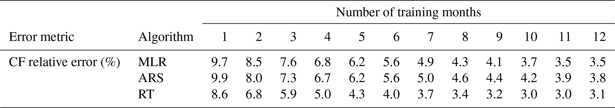
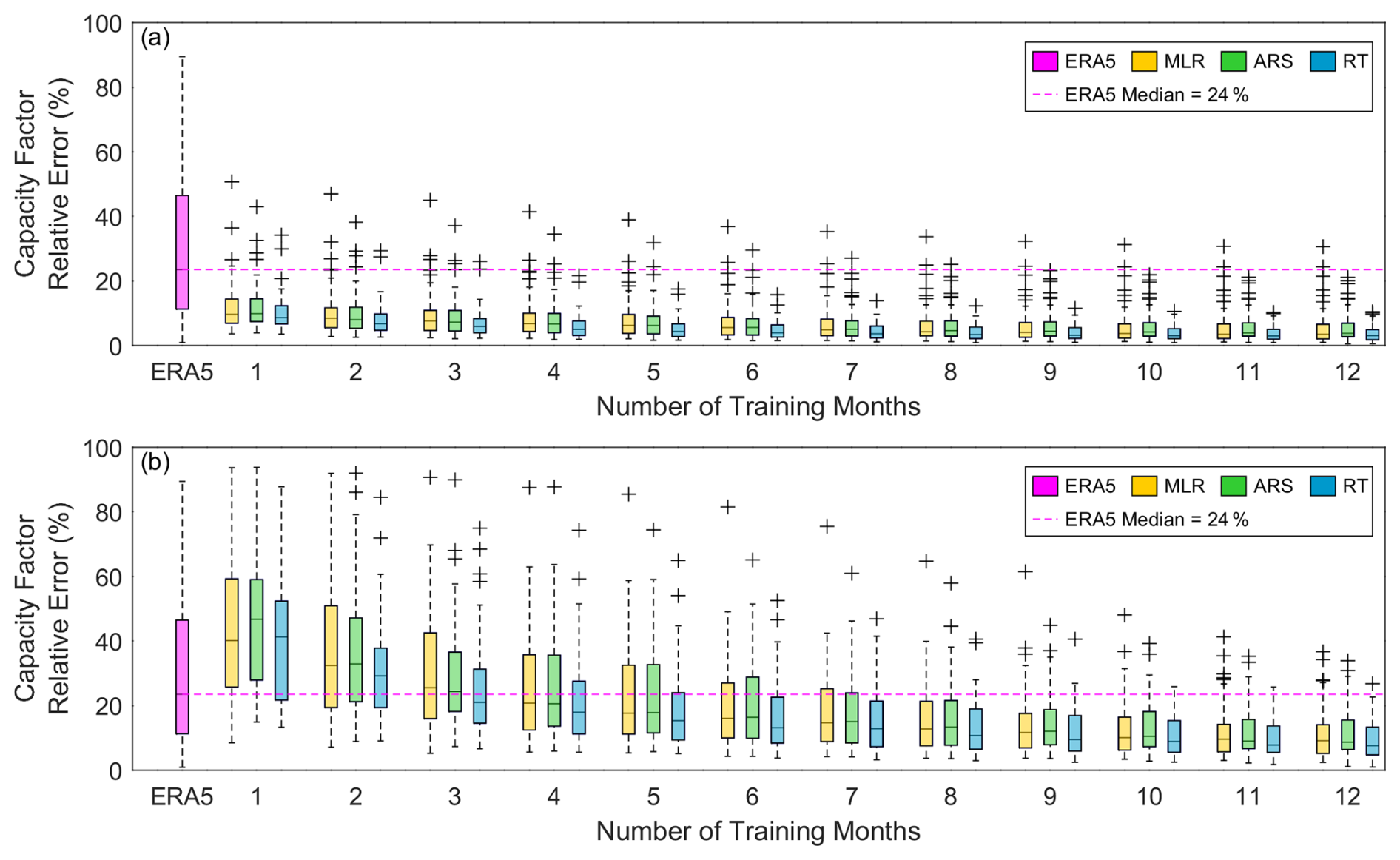
Figure 12 (a) Average and (b) worst-case-scenario capacity factor relative error (| ERA5/MCP capacity factor – capacity factor based on observed wind speeds| /capacity factor based on observed wind speeds) according to number of training months for 58 sites with observation-simulated capacity factors of at least 10 %.

3.5 Performance comparison with higher-resolution wind datasets

ERA5 has shown to be a valuable reference dataset for developing long-term wind speed estimates via MCP with short-term observations thanks to its extensive temporal coverage and relative success at representing fluctuations in observed wind speeds. However, ERA5 has the limitations of coarse horizontal resolution and a tendency to exhibit a slow-wind-speed bias (Ramon et al., 2019; Gualtieri, 2021; Sheridan et al., 2022; Wilczak et al., 2024), which urges comparison of the long-term MCP results with long-term estimates from higher-resolution wind datasets. We explore the performance of the MCP-based long-term wind speed estimates relative to Global Wind Atlas version 3 (GWA3) and the climatology component of the WIND Toolkit Long-term Ensemble Dataset (WTK-LED Climate), for which long-term wind speed estimates are freely and easily accessible through user-friendly web applications.

GWA3 was produced by the Technical University of Denmark (DTU) and the World Bank Group. The developers used the Weather Research and Forecasting (WRF) mesoscale model (Skamarock et al., 2008) in conjunction with the Rapid Radiative Transfer Model (RRTM) for the longwave and shortwave radiation schemes (Mlawer et al., 1997; Iacono et al., 2008), the Mellor–Yamada–Janjić planetary boundary layer (PBL) scheme (Janjić, 1994), and ERA5 as the input and boundary conditions to produce simulated wind data at a horizontal resolution of 3 km (Davis et al., 2023). Next, microscale modeling was performed using the Wind Atlas Analysis and Application Program (WAsP) model (Troen and Petersen, 1989) with an output grid spacing of 250 m for GWA3. GWA3 provides global coverage for land-based wind estimates and offshore wind estimates within 200 km of shorelines. Long-term wind data are output at five heights between 10 and 200 m based on the 10-year period of 2008–2017, and wind speed indices illustrate trends at annual, monthly, and diurnal temporal resolutions. Users can access GWA3 through its web application (DTU, 2024).

WTK-LED Climate was released in 2024 as the wind climatology component, developed by Argonne National Laboratory, of the WIND Toolkit Long-term Ensemble Dataset, a wind resource dataset led by the National Renewable Energy Laboratory. The climatology dataset uses an accelerated version of RRTM for general circulation models (RRTMG) for the radiation schemes, ERA5 for the initial and boundary conditions, and YSU for the PBL scheme (Draxl et al., 2024). WTK-LED Climate covers North America at a 4 km horizontal spatial resolution and 1 h temporal resolution for the 20-year period of 2000–2020. Through the WindWatts web application (NREL, 2024), users can access WTK-LED Climate long-term average and monthly wind speeds at seven output heights between 30 and 140 m.

Across the 66 observation sites, we extract the long-term average wind speed estimates from GWA3 and WTK-LED Climate at the surrounding output heights to the measurement heights and adjust them to the measurement height with the power law (Eqs. 4 and 5). We determine the bias and relative error as in Eqs. (2) and (3), keeping in mind that this comparison involves the different definitions of “long-term” that a user of the GWA3 and WindWatts web applications would experience (10 years for GWA3, 20 years for WTK-LED Climate, and varying lengths for the observations, as shown in Fig. 2b). For our observation sites, the median bias magnitudes for the WTK-LED Climate and GWA3 long-term estimates are 0.71 and 0.36 m s⁻¹, respectively, and the median relative errors are 12.8 % and 6.1 %. On average, using even 1 month of wind speed observations to create long-term MCP-based wind speed estimates provides an improvement in accuracy over the long-term estimates provided by the higher-resolution WTK-LED Climate and GWA3 (Fig. 13, Table 2).

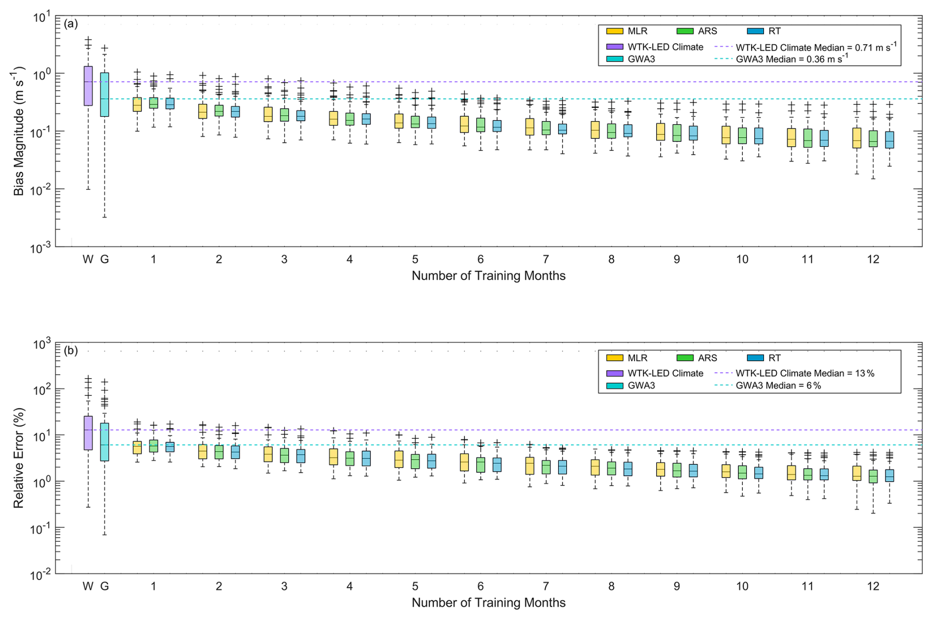
Figure 13 Average long-term wind speed (a) bias magnitude and (b) relative error across 66 sites based on the long-term estimates of GWA3 and WTK-LED Climate and the MCP-based estimates from ERA5 and short-term observations.

3.6 Recommendations and future work

It is important to consider the performance of wind estimation methodologies from a variety of statistical standpoints, since behind-the-meter customers may care most about whether their long-term production meets their initial expectations (bias) and front-of-the-meter customers may also be concerned with distribution network integration with other energy technologies (bias, correlation). While the three MCP algorithms assessed in this study perform similarly in terms of bias magnitude (Fig. 5a), for the shortest training period lengths (1 to 3 months), RT performs significantly worse on average for correlation than MLR and ARS (Fig. 5d).

Given ERA5's popularity in the wind energy community, along with its known challenges in wind speed bias and relative success in terms of wind speed correlation, this study provides a useful framework for evaluating the performance of MCP-based corrections to long-term wind speed estimates using months-long observations. Additionally, the MCP estimates based on short-term observations are found to improve upon the long-term averages of recent wind datasets, including GWA3 and WTK-LED Climate. In the future, the exercise would benefit from expansion to include additional long-term models that provide wind resource information at different horizontal and vertical spatial resolutions. Additionally, the lessons learned in this work are being explored to quantify the geographic extent of their potential application, with aims to support broader wind speed bias correction in distributed wind tools and to reduce the number of onsite measurement sites needed to correct sites with similar wind profile characteristics.

Based on this analysis, we identify the following key recommendations for wind energy developers creating long-term wind resource estimates under the constraint of less than 1 year of onsite measurements which may occur for any number of reasons, including instrument outages or timing of funding opportunities:

• While even 1 month of onsite wind speed measurements improves long-term wind speed estimates on average, incorporating at least 4 months of onsite measurements is a better option to mitigate the errors that could occur if some of the measured and reference wind speeds during the measurement period are poorly correlated.

• Summer months, particularly July and August, should be avoided if opting to create MCP-based wind speed estimates using a single season of measurements in the US, as these months tend to be the least representative of long-term wind speed means and standard deviations.

• Since potential wind customers may care about long-term wind resource accuracy from multiple viewpoints, it is important to note that of the three MCP algorithms explored, RT produces the lowest wind speed and capacity factor relative errors, and ARS yields the lowest wind speed correlations. However, MLR is the least risky algorithm given the possibility of poor correlations between the measurements and the reference data.

The results of this work highlight the potential for anemometer or lidar loan programs to affordably assist future distributed wind energy customers with more accurate long-term wind resource estimates while maximizing the number of customers that can be served by reducing the measurement time needed.