Turbine- and farm-scale power losses in wind farms: an alternative to wake and farm blockage losses

Turbine–wake and farm–atmosphere interactions can reduce wind farm power production. To model farm performance, it is important to understand the impact of different flow effects on the farm efficiency (i.e. farm power normalised by the power of the same number of isolated turbines). In this study we analyse the results of 43 large-eddy simulations (LESs) of wind farms in a range of conventionally neutral boundary layers (CNBLs). First, we show that the farm efficiency η_f is not well correlated with the wake efficiency η_w (i.e. farm power normalised by the power of front-row turbines). This suggests that existing metrics, classifying the loss of farm power into wake loss and farm blockage loss, are not best suited for understanding large wind farm performance. We then evaluate the assumption of scale separation in the two-scale momentum theory (Nishino and Dunstan, 2020) using the LES results. Building upon this theory, we propose two new metrics for wind farm performance: turbine-scale efficiency η_TS, reflecting the losses due to turbine–wake interactions, and farm-scale efficiency η_FS, indicating the losses due to farm–atmosphere interactions. The LES results show that η_TS is insensitive to the atmospheric condition, whereas η_FS is insensitive to the turbine layout. Finally, we show that a recently developed analytical wind farm model predicts η_FS with an average error of 5.7 % from the LES results.

1 Introduction

To meet future energy demands, wind energy capacity will need to increase rapidly. It is likely that individual wind farms will become larger (Veers et al., 2022). When wind turbines are placed together in a farm, they produce less power than in isolation. Predicting this power loss is key for designing wind farms. However, this remains difficult due to the multi-scale nature of wind farm aerodynamics (Porté-Agel et al., 2020).

Behind every turbine is a turbulent wake. When the wakes impact downstream turbines, they can cause significant power losses. Turbine wakes have been investigated extensively using large-eddy simulations (LESs) (e.g. Porté-Agel et al., 2013; Wu and Porté-Agel, 2015; Stevens et al., 2016), wind tunnel experiments (e.g. Vermeer et al., 2003; Bastankhah and Porté-Agel, 2017; Hyvärinen et al., 2018), and field measurements (e.g. Hirth and Schroeder, 2013; Zhan et al., 2020). Data from operational wind farms show that downstream turbines produce less power than the first upstream row (Barthelmie et al., 2010; Nygaard, 2014). Historically, this power degradation has been attributed to turbine–wake interactions.

Large wind farms can act as additional resistance to the atmospheric boundary layer (ABL) (Stevens and Meneveau, 2017). This can act to reduce the wind speed within and upstream of the farm (Porté-Agel et al., 2020). The upstream wind speed reduction is often referred to as the “farm blockage” or “global blockage” effect (Bleeg et al., 2018). LESs of large wind farms (Wu and Porté-Agel, 2017; Allaerts and Meyers, 2017; Lanzilao and Meyers, 2024) show that an internal boundary layer forms in response to the increased flow resistance from the farm. The atmospheric response causes a reduction in “average” wind speed within the farm, in addition to “local” wind speed reduction due to turbine wakes. How much of the downstream power degradation is due to turbine wakes compared to the larger-scale atmospheric response? Recently, Lanzilao and Meyers (2024) performed LESs of large wind farms operating in conventionally neutral boundary layers (CNBLs), where the turbine layout and operating conditions were fixed, but different ABL heights and thermal stratifications above the ABL were tested. Depending on these conditions in the atmosphere, the “wake efficiency” η_w (farm-averaged power normalised by the average power of the first-row turbines) was found to vary significantly from 0.48 to 1.23. This raises the following question: what physical processes are responsible for the different downstream power losses?

An alternative approach to understanding wind farm aerodynamics is the “two-scale momentum theory” developed by Nishino and Dunstan (2020), who proposed splitting the multi-scale problem into “internal” turbine-scale and “external” farm-scale sub-problems. The two sub-problems are coupled together by considering the conservation of momentum and matching the farm-average wind speed. Using the two-scale momentum theory, Kirby et al. (2022) proposed the new concepts of turbine-scale and farm-scale power losses to understand farm performance, where the farm-average wind speed (rather than the wind speed upstream of the farm) plays a key role. The turbine-scale losses are due to farm-internal flow interactions (i.e. turbine–wake interactions), whereas the farm-scale losses are due to the atmospheric response to the whole farm (i.e. reduction in farm-average wind speed).

In this study we compare the two different classifications of wind farm power losses using LESs of large finite-size wind farms. We use the LES results reported by Lanzilao and Meyers (2024) and also perform new simulations with different turbine layouts, which allow us to validate the “two-scale separation” assumption and thus the concepts of turbine- and farm-scale losses. The LES data are available in a public database (Lanzilao and Meyers, 2023b). We first summarise the two-scale momentum theory in Sect. 2. The LES methodology is then briefly described in Sect. 3. A validation of the two-scale separation assumption along with the turbine- and farm-scale losses is presented in Sect. 4. We also compare the farm-scale losses from the wind farm LES with predictions from an analytical wind farm model in Sect. 4. The results are discussed in Sect. 5 and concluding remarks given in Sect. 6.

2 Theory

2.1 Two-scale momentum theory

By considering the momentum balance for a control volume with and without a wind farm present, Nishino and Dunstan (2020) derived the non-dimensional farm momentum (NDFM) equation:

$$\begin{array}{}\text{(1)}& C_{\mathrm{T}}^{*}{\displaystyle \frac{\mathit{\lambda }}{C_{\mathrm{f}\mathrm{0}}}}{\mathit{\beta }}^{\mathrm{2}}+{\mathit{\beta }}^{\mathit{\gamma }}=M,\end{array}$$

where β is the farm wind speed reduction factor that is defined as $\mathit{\beta }\equiv U_{\mathrm{F}}/U_{\mathrm{F}\mathrm{0}}$ (where U_F is the average wind speed in the nominal farm layer of height H_F, and U_F0 is the farm-layer-averaged speed without turbines present); the (farm-averaged) internal turbine thrust coefficient $C_{\mathrm{T}}^{*}$ is defined as $C_{\mathrm{T}}^{*}\equiv {\sum }_{i=\mathrm{1}}^n{T}_i/\frac{\mathrm{1}}{\mathrm{2}}\mathit{\rho }{U}_{\mathrm{F}}^{\mathrm{2}}nA$ (where T_i is the thrust of turbine i, n is the number of turbines in the farm, and A is the rotor-swept area); the array density λ is defined as $\mathit{\lambda }\equiv nA/S_{\mathrm{F}}$ (where S_F is the farm area); the natural surface friction coefficient C_f0 is defined as $C_{\mathrm{f}\mathrm{0}}\equiv {\mathit{\tau }}_{\mathrm{w}\mathrm{0}}/\frac{\mathrm{1}}{\mathrm{2}}\mathit{\rho }{U}_{\mathrm{F}\mathrm{0}}^{\mathrm{2}}$ (where τ_w0 is the bottom shear stress without turbines present); γ is the bottom friction exponent (assumed to be 2.0 in this study, following Nishino and Dunstan (2020), and also as justified later in Sect. 4.2) defined as $\mathit{\gamma }\equiv {\log }_{\mathit{\beta }}({\mathit{\tau }}_{\mathrm{w}}/{\mathit{\tau }}_{\mathrm{w}\mathrm{0}})$ (where τ_w is the bottom shear stress with the turbines present); and M is the momentum availability factor defined by $M\equiv M_{\mathrm{F}}/M_{\mathrm{F}\mathrm{0}}$, where M_F is the net momentum flux into the farm control volume with the turbines present and M_F0 the case without the turbines present. In this study we use a fixed definition of the farm-layer height H_F=2.5H_hub (where H_hub is the turbine hub height) for convenience. The exact value of H_F defined originally by Nishino and Dunstan (2020) depends on the undisturbed wind profile, to ensure that U_F0 matches exactly with the undisturbed wind speed averaged over the turbine-swept area, U_T0; however, as shown later by Kirby et al. (2022), the fixed definition of H_F=2.5H_hub is a good approximation for a wide range of ABL profiles.

Note that the derivation of Eq. (1) given by Nishino and Dunstan (2020) was for an idealised case where the flow through the farm was assumed to be fully developed. However, they also discussed (in Sect. 3 of their paper) how the same form of equation could be derived for more general cases, where the net momentum transfer through the side and top surfaces of the farm control volume should also be considered part of M. See Kirby et al. (2022) for the full expression of M.

Patel et al. (2021) used numerical weather prediction (NWP) simulations to calculate M for a realistic offshore wind farm site in the North Sea. They found, for most cases, an approximately linear relationship between M and β. Therefore, as proposed by Nishino and Dunstan (2020), it is convenient to express M as

$$\begin{array}{}\text{(2)}& M=\mathrm{1}+\mathit{\zeta }(\mathrm{1}-\mathit{\beta }),\end{array}$$

where ζ is called the wind extractability factor. Kirby et al. (2022) showed that ζ was a time-dependent parameter that varied with atmospheric conditions and inversely with farm size. More recently, Kirby et al. (2023b) proposed an analytical model of ζ, as discussed later in Sect. 4.4.

Equations (1) and (2) can be solved to calculate the farm wind speed reduction factor β for a given farm design and atmospheric condition (i.e. λ, $C_{\mathrm{T}}^{*}$, C_f0, γ, and ζ). Using β, the farm power can be calculated using

$$\begin{array}{}\text{(3)}& C_{\mathrm{p}}={\mathit{\beta }}^{\mathrm{3}}{C}_{\mathrm{p}}^{*},\end{array}$$

where the (farm-averaged) turbine power coefficient is defined as $C_{\mathrm{p}}\equiv {\sum }_{i=\mathrm{1}}^n{P}_i/\frac{\mathrm{1}}{\mathrm{2}}\mathit{\rho }{U}_{\mathrm{F}\mathrm{0}}^{\mathrm{3}}nA$ (P_i is the power of turbine i in the farm) and the (farm-averaged) internal turbine power coefficient defined as $C_{\mathrm{p}}^{*}\equiv {\sum }_{i=\mathrm{1}}^n{P}_i/\frac{\mathrm{1}}{\mathrm{2}}\mathit{\rho }{U}_{\mathrm{F}}^{\mathrm{3}}nA$.

2.2 Analytical model of near-ideal wind farm performance

Generally, the internal turbine thrust coefficient $C_{\mathrm{T}}^{*}$ depends on the turbine layout (Kirby et al., 2022). However, as suggested by Nishino (2016) and later confirmed by Kirby et al. (2022), an approximate upper limit of $C_{\mathrm{T}}^{*}$ (with respect to the turbine layout) can be predicted using an analogy to the classical actuator disc theory:

$$\begin{array}{}\text{(4)}& C_{\mathrm{T}}^{*}={\displaystyle \frac{\mathrm{16}{C}_{\mathrm{T}}^{\prime }}{(\mathrm{4}+C_{\mathrm{T}}^{\prime }{)}^{\mathrm{2}}}},\end{array}$$

where $C_{\mathrm{T}}^{\prime }\equiv T_i/\frac{\mathrm{1}}{\mathrm{2}}\mathit{\rho }{U}_{\mathrm{T},i}^{\mathrm{2}}A$ is a turbine resistance coefficient that represents the turbine operating condition (assumed to be constant for all turbines in the farm), and U_T,i is the streamwise velocity averaged across the rotor swept area of turbine i. Note that the two-scale momentum theory summarised in Sect. 2.1 is for general cases where the turbine thrust T_i and power P_i may vary across the farm, whereas the analytical model described here is for less-general cases where the turbine resistance coefficient $C_{\mathrm{T}}^{\prime }$ is constant across the farm (such as the LES cases shown later in this paper, where $C_{\mathrm{T}}^{\prime }$ is fixed at 1.94 for all turbines in the farm). Kirby et al. (2022) showed that, for periodic arrays of turbines with a fixed $C_{\mathrm{T}}^{\prime }$ value of 1.33, some specific turbine layouts could exceed this $C_{\mathrm{T}}^{*}$ value slightly, presumably due to local blockage effects (Ouro and Nishino, 2021; Nishino and Draper, 2015).

The two-scale momentum theory described in Sect. 2.1 can be used, together with Eq. (4), to predict the performance of arrays of actuator discs (or aerodynamically ideal turbines operating below rated conditions). For actuator discs P_i=α_iU_FT_i, where ${\mathit{\alpha }}_i\equiv U_{\mathrm{T},i}/U_{\mathrm{F}}$ is the local wind speed reduction factor, and α_i can be estimated as ${\mathit{\alpha }}_i=\mathit{\alpha }=\sqrt{C_{\mathrm{T}}^{*}/C_{\mathrm{T}}^{\prime }}$ since $C_{\mathrm{T}}^{\prime }$ has been assumed to be constant for all turbines. It is useful to note that this theoretical estimation is strictly valid only for infinite regular arrays of actuator discs. The (farm-averaged) power coefficient of an actuator disc is therefore given by

$$\begin{array}{}\text{(5)}& C_{\mathrm{p}}={\mathit{\beta }}^{\mathrm{3}}\mathit{\alpha }{C}_{\mathrm{T}}^{*}={\mathit{\beta }}^{\mathrm{3}}{C_{\mathrm{T}}^{*}}^{\frac{\mathrm{3}}{\mathrm{2}}}{C_{\mathrm{T}}^{\prime }}^{-\frac{\mathrm{1}}{\mathrm{2}}}.\end{array}$$

Using the analytical model of $C_{\mathrm{T}}^{*}$ (Eq. 4), Eqs. (1), (2), and (5) can be solved to give a theoretical prediction of near-ideal wind farm performance, denoted C_p,Nishino. We describe this as near-ideal since this is close to but slightly less than the maximum possible (as shown later). If we assume γ=2.0, we can derive a single analytical expression for C_p,Nishino, i.e.

$$\begin{array}{}\text{(6)}& \begin{array}{rl}& C_{\mathrm{p},\mathrm{Nishino}}={\displaystyle \frac{\mathrm{64}{C}_{\mathrm{T}}^{\prime }}{(\mathrm{4}+C_{\mathrm{T}}^{\prime }{)}^{\mathrm{3}}}}\times \\ & {\left[{\displaystyle \frac{-\mathit{\zeta }+\sqrt{{\mathit{\zeta }}^{\mathrm{2}}+\mathrm{4}\left(\frac{\mathrm{16}{C}_{\mathrm{T}}^{\prime }}{(\mathrm{4}+C_{\mathrm{T}}^{\prime }{)}^{\mathrm{2}}}\frac{\mathit{\lambda }}{C_{\mathrm{f}\mathrm{0}}}+\mathrm{1}\right)(\mathrm{1}+\mathit{\zeta })}}{\mathrm{2}\left(\frac{\mathrm{16}{C}_{\mathrm{T}}^{\prime }}{(\mathrm{4}+C_{\mathrm{T}}^{\prime }{)}^{\mathrm{2}}}\frac{\mathit{\lambda }}{C_{\mathrm{f}\mathrm{0}}}+\mathrm{1}\right)}}\right]}^{\mathrm{3}}.\end{array}\end{array}$$

Meanwhile, the power coefficient of an isolated turbine C_p,Betz is given by

$$\begin{array}{}\text{(7)}& C_{\mathrm{p},\mathrm{Betz}}={\displaystyle \frac{\mathrm{64}{C}_{\mathrm{T}}^{\prime }}{(\mathrm{4}+C_{\mathrm{T}}^{\prime }{)}^{\mathrm{3}}}},\end{array}$$

which gives a maximum turbine performance of $C_{\mathrm{p},\mathrm{Betz}}=\mathrm{16}/\mathrm{27}$ when $C_{\mathrm{T}}^{\prime }=\mathrm{2.0}$. Note that Eq. (6) reduces to Eq. (7) in two special cases: (i) when $\mathit{\lambda }/C_{\mathrm{f}\mathrm{0}}=\mathrm{0}$ and (ii) when ζ is infinitely large. These two theoretical predictions of performance (C_p,Nishino and C_p,Betz) will be used to define the turbine-scale and farm-scale efficiencies later in Sect. 4.3.

3 Large-eddy-simulation methodology

In this paper we analyse the LESs of wind farms in CNBLs performed by Lanzilao and Meyers (2024) with five new simulation cases. Here we briefly summarise the main details of the LES methodology; for more details, see Lanzilao and Meyers (2024).

The simulations are performed with SP-Wind, an in-house LES code developed at KU Leuven (Allaerts and Meyers, 2017; Lanzilao and Meyers, 2023a). The streamwise (x) and spanwise (y) directions are discretised with a Fourier pseudo-spectral method. For the vertical (z) direction, an energy-preserving fourth-order finite difference scheme is adopted (Verstappen and Veldman, 2003). The effects of subgrid-scale motions on the resolved flow are taken into account with the stability-dependent Smagorinsky model proposed by Stevens et al. (2000), with the Smagorinsky coefficient set to C_s=0.14. The constant C_s is damped near the wall using the damping function proposed by Mason and Thomson (1992).

The turbines are modelled using an actuator disc model with no rotation (Calaf et al., 2010; Meyers and Meneveau, 2010). The turbine forces are projected onto the numerical grid using a Gaussian convolution filter (Calaf et al., 2010). Recently, Shapiro et al. (2019) proposed an additional correction factor for actuator disc models to avoid over-prediction of power and thrust. Unfortunately, this correction factor was not yet included in the LES database of Lanzilao and Meyers (2024), and therefore, it was also not used for the additional cases performed here. Instead, as a next-best approximation, we use the correction factor of Shapiro et al. (2019) in a postprocessing step (see Sect. 4.3 for more details). The turbines have a diameter D of 198 m and a hub height H_hub of 119 m. The thrust is calculated using a disc-based thrust coefficient of $C_{\mathrm{T}}^{\prime }=\mathrm{1.94}$, giving a traditional thrust coefficient of C_T=0.88. A yaw controller is used to keep all turbine discs perpendicular to the incident flow to each turbine.

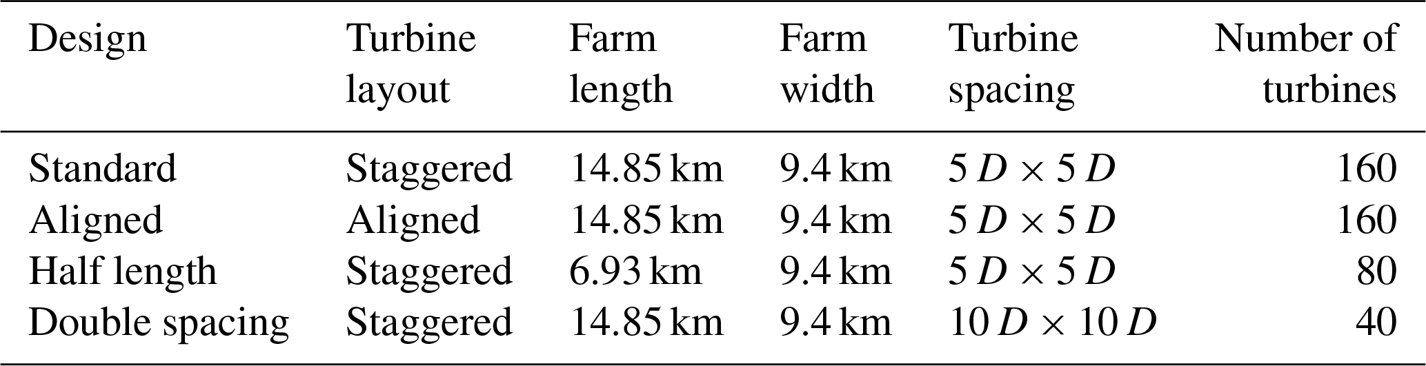
Table 1 summarises the wind farm designs considered in this study. In addition to the “standard” design used by Lanzilao and Meyers (2024), we also consider three additional designs, namely “aligned”, “half length”, and “double spacing”. The standard farm consists of 16 rows and 10 columns of turbines in a staggered layout. The streamwise and spanwise spacing between turbines is 5 D, giving a capacity density of approximately 10 MW km⁻². This is a dense wind farm, but this density is being considered in some development areas. The farm has a length of 14.85 km and a width of 9.4 km. For the three additional farm designs (aligned, half length, and double spacing) the turbine layout, farm length, and turbine spacing were changed, respectively, from the standard design (Table 1). Note that the farm length is the distance between the first and last turbine rows, and the half-length case has 8 rows rather than 16 rows. For all simulations the computational domain size is $L_x\times L_y\times L_z=\mathrm{50}$ km × 30 km × 25 km. The grid resolution is Δx=31.25 m, Δy=21.74 m, and Δz=5 m in the lowest 1.5 km of the domain, following the set-up used by Lanzilao and Meyers (2024).

Table 1 A summary of wind farm designs considered in this study.

The bottom boundary conditions are given by the classical Monin–Obukhov similarity theory for neutral boundary layers (Moeng, 1984). Periodic boundary conditions are applied at the streamwise and spanwise edges of the domain. To break the streamwise periodicity and impose an inflow condition, we use the wave-free fringe region technique (Lanzilao and Meyers, 2023a). At the top of the domain, a rigid-lid condition is used, which imposes zero shear stress and vertical velocity and a fixed potential temperature. To minimise gravity-wave reflection, we adopt a Rayleigh damping layer in the upper part of the domain (Lanzilao and Meyers, 2023a).

Table 2 A summary of atmospheric stratifications considered in this study.

The atmospheric stratification is varied by changing the capping inversion height, capping inversion strength, and free-atmosphere lapse rate. Table 2 shows a summary of the different atmospheric stratifications. All combinations of these parameters were considered for the standard farm design by Lanzilao and Meyers (2024). We use the notation introduced by Lanzilao and Meyers (2024); e.g. H500-C5-G4 refers to a capping inversion height of 500 m, capping inversion strength of 5 K, and free-atmosphere lapse rate of 4 K km⁻¹.

In this study we fix the geostrophic wind to 10 m s⁻¹, which is in line with previous studies (Abkar and Porté-Agel, 2013; Wu and Porté-Agel, 2017; Allaerts and Meyers, 2017; Lanzilao and Meyers, 2022). This value is also chosen so that all turbines operate below their rated wind speed, justifying the use of the constant thrust coefficient noted earlier. Finally, we fix the Coriolis frequency to $f_{\mathrm{c}}=\mathrm{1.14}\times {\mathrm{10}}^{\mathrm{-}\mathrm{4}}$ s⁻¹ and the surface roughness to $z_{\mathrm{0}}=\mathrm{1}\times {\mathrm{10}}^{\mathrm{-}\mathrm{4}}$ m for all simulations.

4 Results

In the following we first investigate the wake and farm-blockage losses observed in the LES performed by Lanzilao and Meyers (2024) in Sect. 4.1. We then present in Sect. 4.2 a validation of the two-scale separation assumption in the two-scale momentum theory proposed by Nishino and Dunstan (2020). We apply the concepts of turbine-scale and farm-scale losses (Kirby et al., 2022) to the LES results in Sect. 4.3. Finally, we assess the accuracy of an analytical model (Kirby et al., 2023b) in predicting the farm-scale losses.

4.1 Wake and farm blockage losses

Here we reanalyse the results of the wind farm LES performed by Lanzilao and Meyers (2024), who reported that the farm normalised power relative to the first-row power (i.e. wake efficiency) varied from 0.48 to 1.23 for the same turbine layout and wind direction. The aim of this section is therefore to investigate the physical mechanisms behind such a large change in the farm normalised power.

Allaerts and Meyers (2018) have introduced three different “efficiencies” (or power ratios) for wind farm performance. Firstly, the wake efficiency η_w (sometimes called “normalised power”) is defined as

$$\begin{array}{}\text{(8)}& {\mathit{\eta }}_{\mathrm{w}}\equiv {\displaystyle \frac{P_{\mathrm{farm}}}{P_{\mathrm{1}}}},\end{array}$$

where P_farm is the farm-averaged turbine power, and P₁ is the first-row-averaged turbine power. Secondly, the “non-local” efficiency η_nl is defined as

$$\begin{array}{}\text{(9)}& {\mathit{\eta }}_{\mathrm{nl}}\equiv {\displaystyle \frac{P_{\mathrm{1}}}{P_{\mathrm{\infty }}}},\end{array}$$

where P_∞ is the power output of an isolated turbine under the same atmospheric conditions. This represents the power loss due to the velocity reduction in front of the farm, i.e. due to farm blockage. Finally the “farm efficiency” η_f is defined as

$$\begin{array}{}\text{(10)}& {\mathit{\eta }}_{\mathrm{f}}\equiv {\displaystyle \frac{P_{\mathrm{farm}}}{P_{\mathrm{\infty }}}}\equiv {\mathit{\eta }}_{\mathrm{w}}{\mathit{\eta }}_{\mathrm{nl}}.\end{array}$$

The farm efficiency η_f quantifies the overall power losses caused by placing turbines together in a farm.

As noted by Lanzilao and Meyers (2024), the farm LES results show a relatively strong negative correlation between η_w and η_nl (Fig. 1). When the farm blockage increases (i.e. η_nl decreases), the downstream power losses decrease (i.e. η_w increases). These two effects counteract each other to a certain extent. This means that η_w is affected by not only turbine–wake interactions but also larger farm-scale flow effects causing farm blockage.

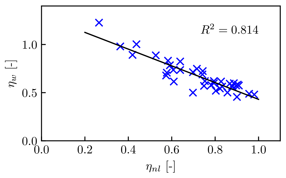
Figure 1 Relationship between wake efficiency η_w and non-local efficiency η_nl for all 38 LES cases from Lanzilao and Meyers (2024). The R² value shows the coefficient of determination.

The correlation between η_w and η_nl is caused by the induced pressure gradients across the farm. To illustrate this, the pressure perturbation for cases H300-C2-G1 and H300-C8-G1 is shown in Fig. 2. Case H300-C2-G1 has a low degree of farm blockage (η_nl=0.857) and a relatively small induced pressure gradient. Conversely, H300-C8-G1 has a high degree of farm blockage (η_nl=0.437) and a large induced pressure gradient. Essentially, H300-C8-G1 has a larger driving force across the farm, meaning that the velocity tends to stay high across the farm despite the lower velocity at the front. This causes η_w to be higher (η_w=1.00 compared to η_w=0.501 for H300-C2-G1).

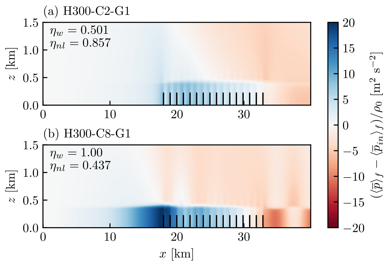
Figure 2 Time-averaged pressure perturbation averaged across the farm width for cases (a) H300-C2-G1 and (b) H300-C8-G1.

The LES results also show that the overall farm efficiency η_f is not well correlated with either the wake efficiency η_w or the non-local efficiency η_nl. Figure 3a shows the weak correlation between η_f and η_w. This shows that the wake efficiency or normalised power is not a good indicator of wind farm efficiency. The correlation between η_f and η_nl is also relatively weak, as shown in Fig. 3b. The negative farm blockage effect is mostly counteracted by the increased pressure gradient across the farm, which increases η_w.

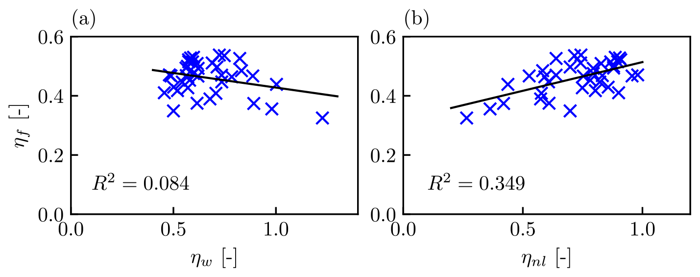
Figure 3 (a) Relationship between farm efficiency η_f and wake efficiency η_w and (b) relationship between farm efficiency η_f and non-local efficiency η_nl, for all 38 LES cases from Lanzilao and Meyers (2024). The R² values show the coefficients of determination.

To better understand why the same turbine layout results in a very wide range of η_w from 0.48 to 1.23, now we will investigate whether this could be explained by either (1) different “effective” turbine layouts caused by changes in local wind directions within the farm or (2) different wake recovery rates. In the following, we will again focus on the two illustrative cases, H300-C2-G1 and H300-C8-G1. The capping inversion height is the same for both, but H300-C2-G1 gives η_w=0.501, whereas H300-C8-G1 gives η_w=1.00.

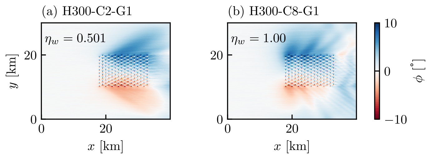
Figure 4 Time-averaged flow angle at the turbine hub height for cases (a) H300-C2-G1 and (b) H300-C8-G1.

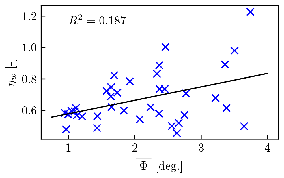
Figure 5 Relationship between wake efficiency η_w and the farm-averaged magnitude of turbine yaw angle $\stackrel{\mathrm{‾}}{\left|\mathrm{\Phi }\right|}$ for all 38 LES cases from Lanzilao and Meyers (2024). The R² value shows the coefficient of determination.

First, we show that the large difference in η_w cannot be explained by different effective turbine layouts. The local flow direction for cases H300-C2-G1 and H300-C8-G1 is shown in Fig. 4. Both cases have an outward flow direction of approximately 5° at the sides. However, both cases have similar variations in the local flow directions across the farm. Figure 5 shows there is not a strong relationship between η_w and the farm-averaged absolute turbine yaw angle $\stackrel{\mathrm{‾}}{\left|\mathrm{\Phi }\right|}$ for all 38 cases, indicating that the large variation in η_w cannot be explained by the change in effective turbine layout.

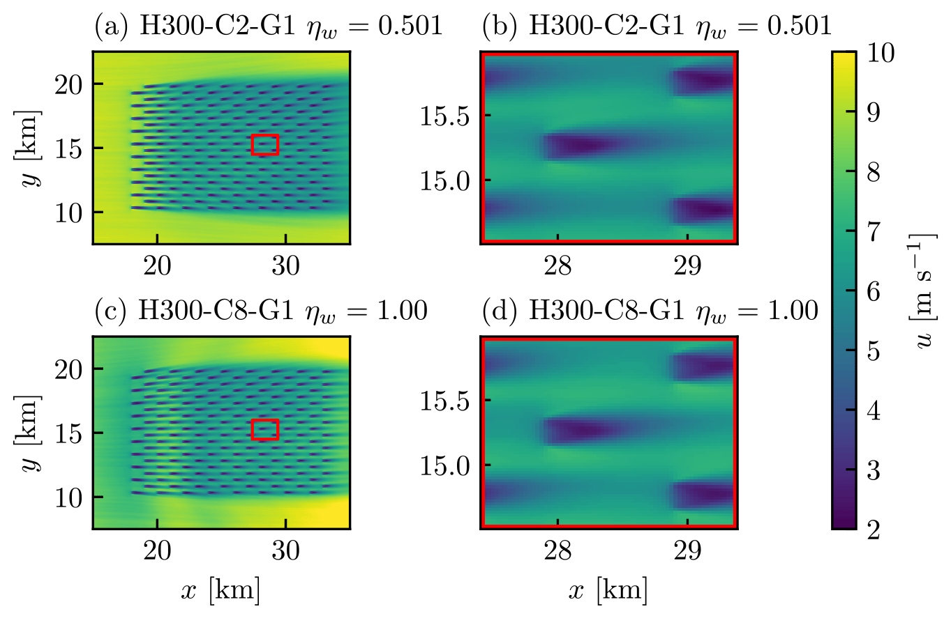
Figure 6 Time-averaged u velocity contours at the turbine hub height for case H300-C2-G1 (a) across the whole farm and (b) inside the farm and for case H300-C8-G1 (c) across the whole farm and (d) inside the farm.

Next, we show that the wake recovery behind each turbine is also uncorrelated with the wake efficiency η_w. The farm flow profiles are shown in Fig. 6a for H300-C2-G1 and in Fig. 6c for H300-C8-G1. The individual wake deficits look similar, but rather it is the farm-scale flows that are different. A closer view of individual wakes towards the centre of the farm is shown in Fig. 6b and d. Despite one case having η_w=0.501 and the other having η_w=1.00, the wakes look almost identical. This suggests that the characteristics of individual turbine wake recovery are not contributing to the difference in η_w.

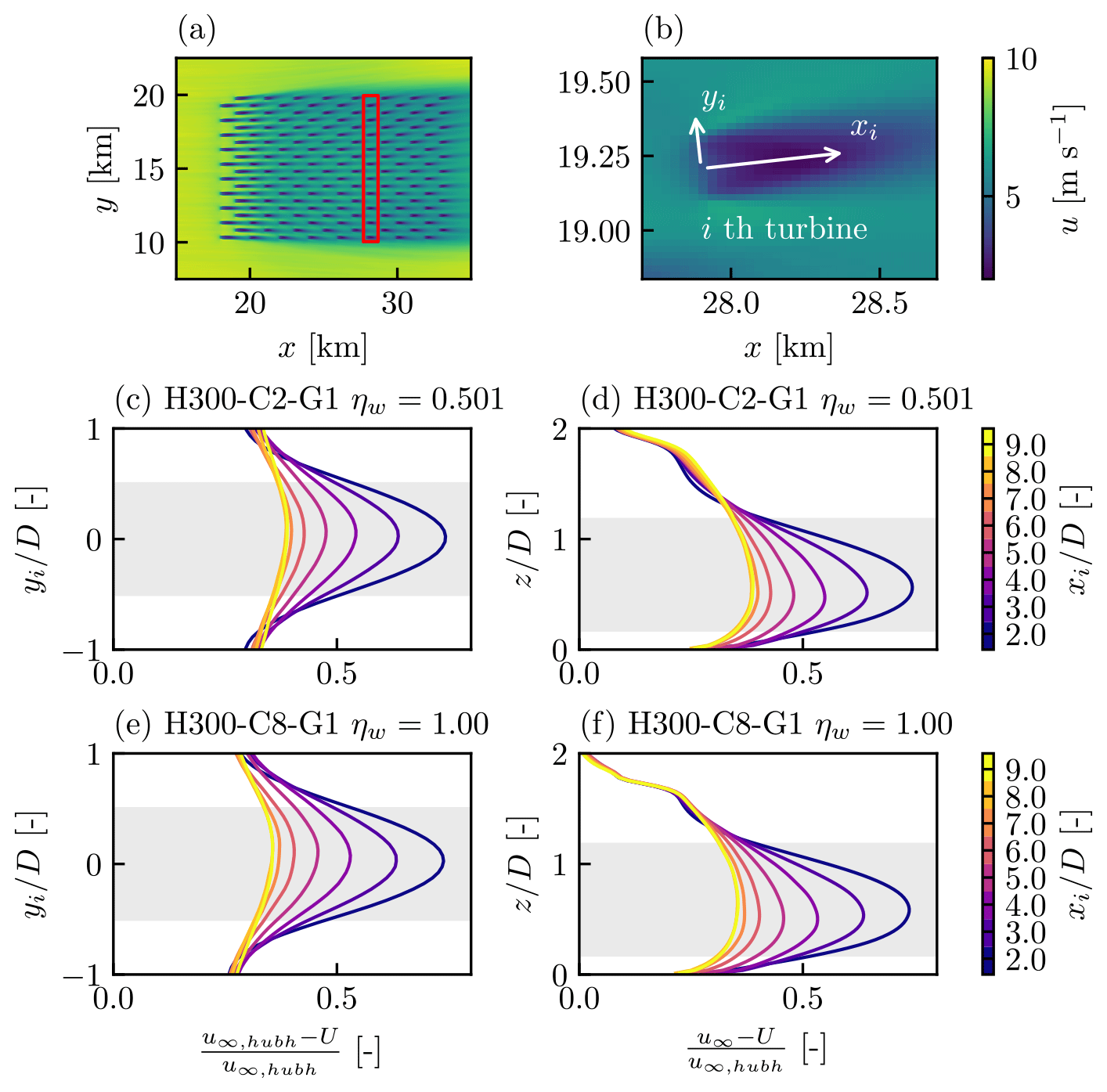
Figure 7 (a) Time-averaged u velocity contours at the turbine hub height for case H300-C2-G1, with the 11th row highlighted in red, and (b) new local coordinates x_i and y_i. Normalised wake velocity deficit profiles averaged for all 10 turbines in the 11th row, plotted in the horizontal (y_i) direction at the hub height and in the vertical (z) direction through the rotor centre for (c), (d) case H300-C2-G1 and (e), (f) case H300-C8-G1, respectively.

A more quantitative comparison in Fig. 7 shows that both cases have similar wake velocity deficits. Here we calculated the wake velocity deficit by defining new coordinates x_i and y_i local to each turbine (see Fig. 7b). x_i is perpendicular to each rotor and y_i parallel. We averaged the wake velocity deficits (relative to the undisturbed velocity u_∞(z) recorded in the precursor simulation) for each turbine in the 11th row. This row was chosen because the flow profiles are characteristic of the average flow profile across the entire farm. Figure 7c–f show that both horizontal and vertical wake deficit profiles are approximately Gaussian, and the wake deficit profiles and wake recovery rate are both similar. H300-C8-G1 has a slightly smaller normalised wake velocity deficit compared to H300-C2-G1, but this is not sufficient to explain the large difference in η_w values.

The wake recovery across the entire farm is also similar for the two cases. We calculated the wake width by fitting a Gaussian function to the wake deficit profiles shown in Fig. 7. Note that the centre of the Gaussian function was not fixed to the rotor centre. The wake width σ was calculated as the geometric mean of the wake width in the horizontal σ_y and vertical σ_z directions, i.e. $\mathit{\sigma }=\sqrt{{\mathit{\sigma }}_y{\mathit{\sigma }}_z}$. The wake width as a function of the downstream distance for turbine rows 3 to 16 is shown in Fig. 8. The first two rows were excluded, as the wake recovery was much slower. An approximately linear growth in wake width can be seen for both cases. We calculated the wake expansion coefficient k^* using the equation $\mathit{\sigma }/D=k^{*}{x}_i/D+\mathit{ϵ}$ where ϵ is the initial wake width. We then averaged the value of k^* across the 3rd to 16th rows to obtain a farm-averaged k^*, which is shown in Fig. 8. The value of k^* was found to be higher than the values reported by Bastankhah and Porté-Agel (2014). This is presumably because the turbulence levels are higher within a large wind farm. Most importantly, the average wake growth rate is higher for the case with the lower value of η_w. This again demonstrates that η_w is not strongly related to local wake recovery behind each turbine.

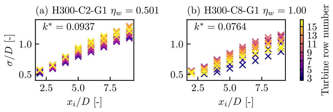
Figure 8 Normalised wake width with streamwise distance for different turbine rows for cases (a) H300-C2-G1 and (b) H300-C8-G1.

Figure 9 (a) Relationship between farm efficiency η_f and farm-averaged k^*, (b) relationship between wake efficiency η_w and farm-averaged k^*, and (c) relationship between wake efficiency η_w and farm-averaged wake width at 10 D downstream of each disc. R² shows the coefficient of determination.

To confirm this trend further, we calculated the farm-averaged wake expansion coefficient k^* and normalised wake width $\mathit{\sigma }/D$ (at 10 D downstream of each disc) for 29 of the farm LES cases from Lanzilao and Meyers (2024). The cases with the lowest capping inversion (150 m) were excluded, as they did not have Gaussian wake deficit profiles in the vertical direction due to the vicinity of the capping inversion base to the turbine-tip height. Figure 9a shows that there is no correlation between the farm efficiency η_f and the wake expansion coefficient k^*. Figure 9b shows that low η_w values cannot be explained by a slower wake recovery. On the contrary, these LES results show that cases with a low η_w value tend to have a faster wake recovery. This trend can also be confirmed from the negative correlation between η_w and the farm-averaged turbine wake width (at 10 D downstream of each disc) shown in Fig. 9c.

The wake efficiency η_w has been extensively used to analyse farm performance, as it is a relatively easy parameter to calculate, e.g. using supervisory control and data acquisition (SCADA). However, these LES results (for a fixed staggered turbine layout with different ABL conditions) suggest that this wake efficiency parameter η_w is not a good indicator of the turbine–wake interactions within the farm.

4.2 Validation of the two-scale separation assumption

The two-scale momentum theory provides an alternative way of understanding wind farm performance. This theory is particularly useful when the two-scale separation assumption is valid, meaning that the farm internal parameters ($C_{\mathrm{T}}^{*}$ and γ) depend only on internal or turbine-scale conditions, whereas the external parameter (ζ) depends only on external or farm-scale conditions. This assumption allows the turbine-scale and farm-scale flows to be modelled separately; however, this assumption has not been fully evaluated in previous studies. In the following we present a first validation of the two-scale separation assumption using four new LES results as well as the previous LES results from Lanzilao and Meyers (2024).

Here we calculate ζ_LES from the momentum availability factor M_LES and the farm wind speed reduction factor β_LES obtained from the LES as follows:

$$\begin{array}{}\text{(11)}& {\mathit{\zeta }}_{\mathrm{LES}}={\displaystyle \frac{M_{\mathrm{LES}}-\mathrm{1}}{\mathrm{1}-{\mathit{\beta }}_{\mathrm{LES}}}},\end{array}$$

where β_LES is calculated directly from the values of U_F and U_F0 obtained from the LES, whereas M_LES is calculated as

$$\begin{array}{}\text{(12a)}& {\displaystyle }{M}_{\mathrm{LES}}={\displaystyle \frac{{\sum }_{i=\mathrm{1}}^n{T}_i+{\mathit{\tau }}_{\mathrm{w}}S}{{\mathit{\tau }}_{\mathrm{w}\mathrm{0}}S}}\text{(12b)}& {\displaystyle }={\displaystyle \frac{{\sum }_{i=\mathrm{1}}^n{T}_i}{{\mathit{\tau }}_{\mathrm{w}\mathrm{0}}S}}+{{\mathit{\beta }}_{\mathrm{LES}}}^{\mathit{\gamma }}\text{(12c)}& {\displaystyle }={\displaystyle \frac{\mathit{\lambda }{C}_{\mathrm{T},\mathrm{LES}}^{*}}{C_{\mathrm{f}\mathrm{0}}}}{{\mathit{\beta }}_{\mathrm{LES}}}^{\mathrm{2}}+{{\mathit{\beta }}_{\mathrm{LES}}}^{\mathit{\gamma }}.\end{array}$$

The bottom friction exponent γ was not recorded in the present LES results, but we can expect that this varies between 1.5 and 2.0 (Kirby et al., 2022). Considering Eq. (12c), a typical value of $\mathit{\lambda }{C}_{\mathrm{T}}^{*}/C_{\mathrm{f}\mathrm{0}}$ is 17.5 for the farms in this study, meaning that the total force due to turbine thrust is much larger than the force due to the bottom friction (and hence, the impact of γ is very small). For example, if we suppose that β=0.75, using γ=1.5 gives M_LES=10.5, whereas γ=2.0 gives M_LES=10.4. Since the value of M_LES is largely insensitive to the value of γ, we will use γ=2.0 in the following analysis.

Figure 10 shows the relationship between M_LES and β_LES obtained for three different atmospheric conditions. As can be seen from the figure, the wind extractability factor ζ_LES changes with the atmospheric conditions, but it is not sensitive to the turbine layout. The aligned turbine layouts result in a lower wind speed reduction (i.e. lower value of 1−β_LES) because they present a lower flow resistance. However, the value of ζ_LES is almost identical for aligned and staggered layouts under a given atmospheric condition. A farm with a staggered layout but doubled turbine spacing (10 D×10 D) also follows approximately the same relationship (see Fig. 10b). This demonstrates that the linear relationship is valid for a wide range of β. It can also be seen that ζ_LES decreases with decreasing capping inversion height. This trend was predicted by the theoretical model of ζ proposed by Kirby et al. (2023b). The values of ζ_LES for all atmospheric conditions tested in this study are shown in Fig. 11a. As shown theoretically by Nishino and Dunstan (2020), for a given wind farm, there is a positive monotonic relationship between ζ and wind farm efficiency. Therefore the effects of different atmospheric conditions on the wind farm efficiency reported by Lanzilao and Meyers (2024) can be explained by different wind extractability factors ζ.

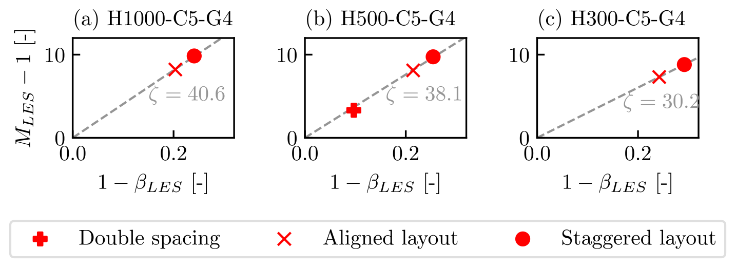
Figure 10 Relationship between momentum availability factor M_LES and farm wind speed reduction factor β_LES for the (a) H1000-C5-G4, (b) H500-C5-G4, and (c) H300-C5-G4 atmospheric conditions.

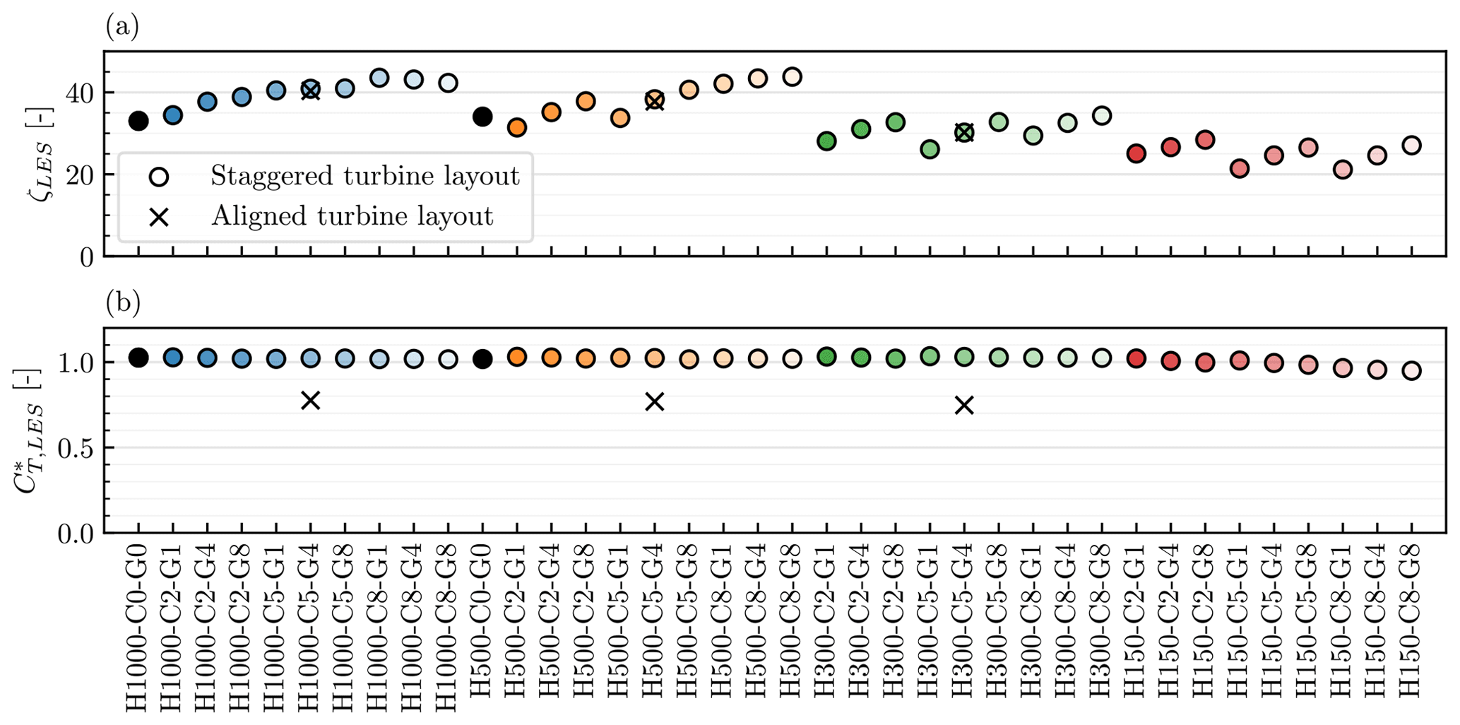
Figure 11 Values of (a) wind extractability factor ζ and (b) internal turbine thrust coefficient $C_{\mathrm{T}}^{*}$ for all atmospheric conditions tested.

The LES results also show that the internal turbine thrust coefficient $C_{\mathrm{T},\mathrm{LES}}^{*}$ is insensitive to atmospheric conditions (Fig. 11b). Apart from the lowest capping inversion cases (H150), the staggered turbine layout consistently gives a high $C_{\mathrm{T},\mathrm{LES}}^{*}$ value of about 1.0 irrespective of atmospheric stratification (Fig. 11b), whereas the aligned turbine layout consistently gives a lower $C_{\mathrm{T},\mathrm{LES}}^{*}$ value than the staggered one. This trend is expected, as Kirby et al. (2022) showed that increased turbine–wake interactions reduce the value of $C_{\mathrm{T}}^{*}$. Turbine–wake interactions reduce $C_{\mathrm{T}}^{*}$ because the waked turbines experience a lower incident wind speed and so produce less thrust.

These LES results in Figs. 10 and 11 strongly indicate that the assumption of two-scale separation is valid for large finite wind farms, at least in the practical range of CNBLs tested in this study. This means that the impact of turbine-scale flows (i.e. turbine–wake interactions) and farm-scale flows (i.e. farm–atmosphere interaction) could be modelled separately through the modelling of $C_{\mathrm{T}}^{*}$ and ζ, as suggested originally by Nishino and Dunstan (2020), to predict wind farm power in a less complicated and more physically meaningful manner.

4.3 Turbine-scale and farm-scale power losses

Turbine-scale and farm-scale power losses (Kirby et al. (2022); see also Stevens (2023)) are alternative metrics for wind farm performance, as illustrated in Fig. 12. The turbine-scale power losses are due to the internal flow interactions within the farm (i.e. turbine–wake interactions). Farm-scale power losses are due to the interaction between the ABL and the farm as a whole. Kirby et al. (2022) have shown, using LESs of flow over a periodic array of actuator discs for 50 different layouts, that the near-ideal farm performance predicted by Eq. (6) is a good measure to differentiate the turbine-scale power losses from the farm-scale power losses. Note that when each turbine in a wind farm generates its wake, the flow bypassing the turbine locally accelerates due to the conservation of mass (at each turbine scale); hence, we consider that any reduction in farm-average wind speed is caused by external (farm–atmosphere) interactions. This means that the power losses accompanied by a reduction in farm-average wind speed are farm-scale power losses (caused by external interactions) and not turbine-scale power losses (caused by internal interactions).

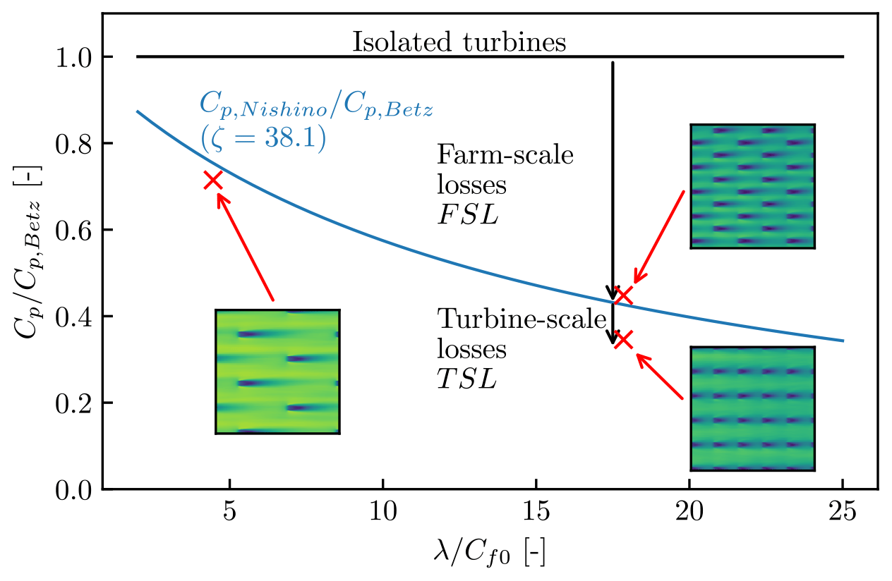
Figure 12 Schematic of the overall farm efficiency $C_{\mathrm{p}}/C_{\mathrm{p},\mathrm{Betz}}$ against the effective array density $\mathit{\lambda }/C_{\mathrm{f}\mathrm{0}}$, illustrating farm-scale and turbine-scale power losses. The blue line shows the near-ideal farm performance predicted by the two-scale momentum theory for a given set of conditions (corresponding to Fig. 10b with ζ=38.1), whereas the red crosses show the results of the three farm LES cases discussed in Fig. 10b.

It should also be noted that the 50 LES results of Kirby et al. (2022) are for idealised infinitely large wind farms; hence, their findings are not directly applicable to finite-sized farms in general. However, as shown in the previous section, our new LES results indicate that the internal thrust coefficient $C_{\mathrm{T}}^{*}$ is insensitive to external conditions. This means that the upper limit of $C_{\mathrm{T}}^{*}$ (with respect to the turbine layout for a given value of C_T’) should also be insensitive to external conditions, supporting our argument that the near-ideal farm performance predicted by Eq. (6) is a good measure for finite farms as well.

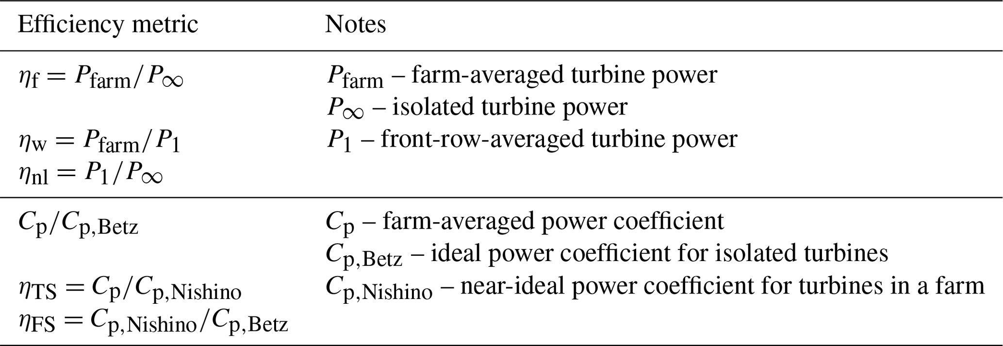
Here we propose a slight modification to the new metrics for wind farm performance introduced by Kirby et al. (2022), namely the “turbine-scale efficiency” η_TS and “farm-scale efficiency” η_FS¹ defined as

$$\begin{array}{}\text{(13)}& {\displaystyle }{\mathit{\eta }}_{\mathrm{TS}}\equiv {\displaystyle \frac{C_{\mathrm{p}}}{C_{\mathrm{p},\mathrm{Nishino}}}}\text{(14)}& {\displaystyle }{\mathit{\eta }}_{\mathrm{FS}}\equiv {\displaystyle \frac{C_{\mathrm{p},\mathrm{Nishino}}}{C_{\mathrm{p},\mathrm{Betz}}}}.\end{array}$$

η_TS and η_FS are related to the overall wind farm efficiency $C_{\mathrm{p}}/C_{\mathrm{p},\mathrm{Betz}}$ by

$$\begin{array}{}\text{(15)}& {\displaystyle \frac{C_{\mathrm{p}}}{C_{\mathrm{p},\mathrm{Betz}}}}\equiv {\mathit{\eta }}_{\mathrm{TS}}{\mathit{\eta }}_{\mathrm{FS}}.\end{array}$$

Note that $C_{\mathrm{p}}/C_{\mathrm{p},\mathrm{Betz}}$ is slightly different from the overall farm efficiency η_f used by Lanzilao and Meyers (2024). Here we normalise by the turbine performance predicted using the actuator disc theory, C_p,Betz, for a given turbine resistance coefficient ($C_{\mathrm{T}}^{\prime }=\mathrm{1.94}$ in this study). This is instead of the isolated turbine power found using the LES, P_∞, which is slightly different from the power predicted by the actuator disc theory. We normalised all values by C_p,Betz to ensure that the predicted power coefficients from the LES, C_p, and the theory, C_p,Nishino, are normalised by the same value. A summary of the efficiency metrics used in this study is given in Table 3.

As can be seen from Eq. (15), the overall farm efficiency is the product of turbine-scale efficiency η_TS and farm-scale efficiency η_FS. For convenience, we can also introduce an alternative set of metrics, namely the turbine-scale loss (TSL) defined in Eq. (16) and farm-scale loss (FSL) defined in Eq. (17). The only difference from η_TS and η_FS is that TSL and FSL both have the same denominator, C_p,Betz. This allows the two losses to be simply added up (instead of multiplied) to obtain the total loss in Eq. (18).

$$\begin{array}{}\text{(16)}& {\displaystyle }\mathrm{TSL}\equiv {\displaystyle \frac{C_{\mathrm{p},\mathrm{Nishino}}-C_{\mathrm{p}}}{C_{\mathrm{p},\mathrm{Betz}}}}\equiv {\mathit{\eta }}_{\mathrm{FS}}\left(\mathrm{1}-{\mathit{\eta }}_{\mathrm{TS}}\right)\text{(17)}& {\displaystyle }\mathrm{FSL}\equiv {\displaystyle \frac{C_{\mathrm{p},\mathrm{Betz}}-C_{\mathrm{p},\mathrm{Nishino}}}{C_{\mathrm{p},\mathrm{Betz}}}}\equiv \mathrm{1}-{\mathit{\eta }}_{\mathrm{FS}}\text{(18)}& {\displaystyle \frac{C_{\mathrm{p}}}{C_{\mathrm{p},\mathrm{Betz}}}}\equiv \mathrm{1}-\left(\mathrm{TSL}+\mathrm{FSL}\right)\end{array}$$

Table 3 A summary of wind farm efficiency metrics.

In this study we calculate η_TS and η_FS using ζ_LES obtained from each LES case. Shapiro et al. (2019) proposed a correction factor N for the overpredicted velocity through an actuator disc as

$$\begin{array}{}\text{(19)}& N={\left(\mathrm{1}+{\displaystyle \frac{C_{\mathrm{T}}^{\prime }}{\mathrm{2}}}{\displaystyle \frac{\mathrm{1}}{\sqrt{\mathrm{3}\mathit{\pi }}}}{\displaystyle \frac{\mathrm{\Delta }}{D}}\right)}^{-\mathrm{1}},\end{array}$$

where Δ is the Gaussian kernel width used for projecting turbine forces onto the numerical grid. In this study Δ=32.61 m in the y and z directions, which gives N=0.950, meaning that the turbine thrust and power are corrected by N² and N³, respectively. Since the correction factor of Shapiro et al. (2019) was not implemented in the LES, we apply it here as a postprocessing step to correct for possible overpredictions of power and thrust.

To calculate η_TS and η_FS we used the procedure summarised in Fig. 13. Essentially, we solved Eqs. (1) and (2) for β using ζ=ζ_LES and the parameter values in Table 4. Note that we used $\mathrm{0.88}/N^{\mathrm{2}}=$ 0.974 as the value of $C_{\mathrm{T}}^{*}$, which has been corrected (i.e. adjusted upwards) to account for LES resolution effects. The 5D×5D turbine spacing gives an array density λ of 0.0314. The value of the farm-layer height is given by H_F=2.5H_hub, and for the turbines, simulated H_hub is 119 m. $C_{\mathrm{p},\mathrm{Nishino}}/C_{\mathrm{p},\mathrm{Betz}}$ is given by the value of β³.

Table 4 Parameter values used to calculate turbine-scale efficiency η_TS and farm-scale efficiency η_FS.

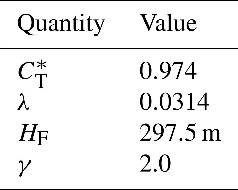
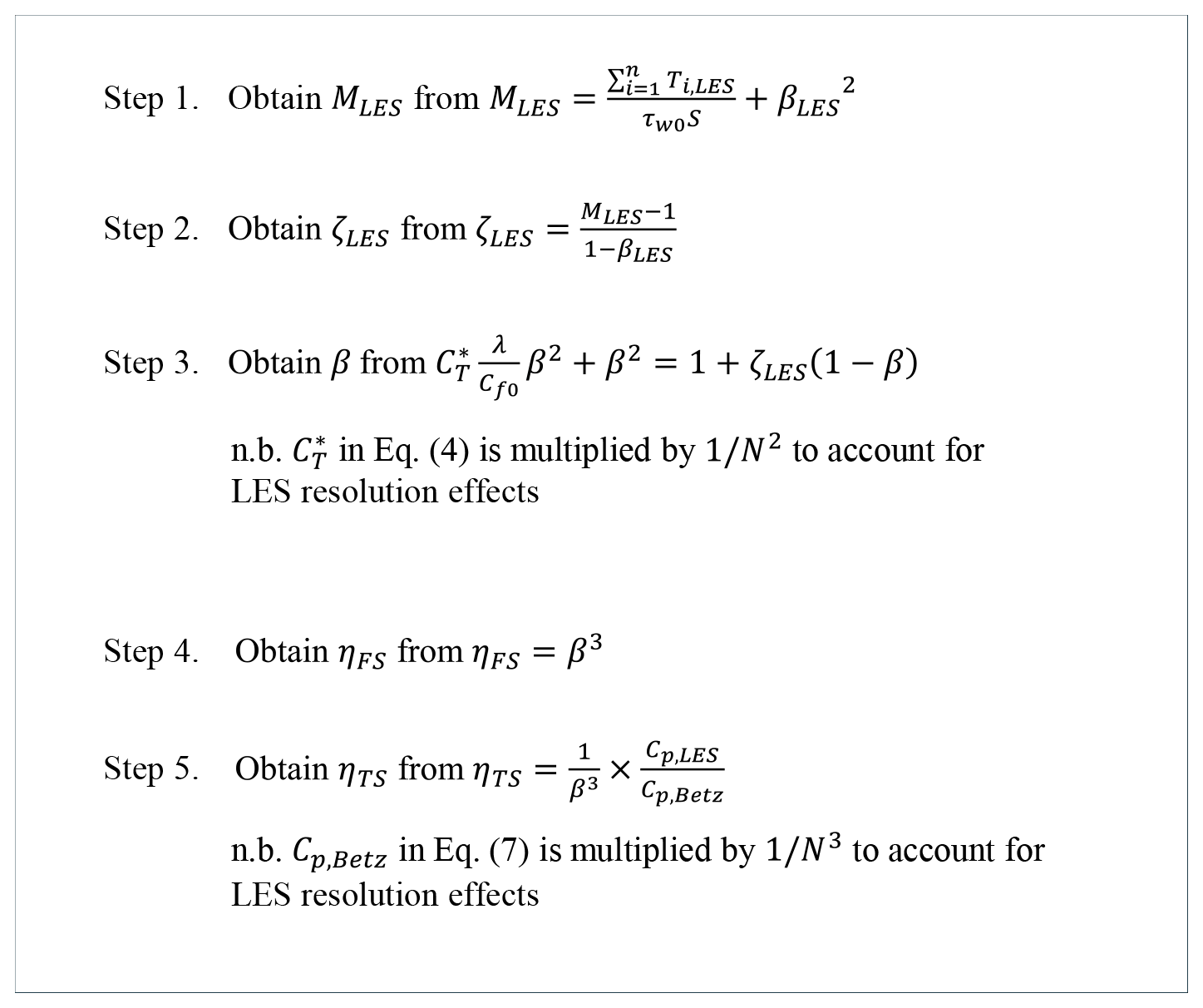
Figure 13 Procedure used to calculate turbine-scale efficiency η_TS and farm-scale efficiency η_FS. Note that $C_{\mathrm{T}}^{*}$ required in step 3 is not $C_{\mathrm{T},\mathrm{LES}}^{*}$ in Fig. 11 but the theoretical $C_{\mathrm{T}}^{*}$ given by Eq. (4). This is because the aim here is to obtain β for the near-ideal (hypothetical) wind farm subjected to a given wind extractability factor ζ_LES (obtained from LES using steps 1 and 2).

Figure 14 compares the farm performance for three different atmospheric conditions (including the two cases discussed earlier in Sect. 4.1) for demonstration. As can be seen from Fig. 14a, the wake and non-local efficiencies are both sensitive to capping inversion strength. These two effects mostly cancelled each other out, giving similar farm efficiencies for these three cases. Conversely, Fig. 14b shows that the turbine-scale efficiency η_TS is almost unchanged for the three cases. This reflects the fact that the turbine layout was unchanged, so the turbine-scale flows were very similar (as shown earlier in Fig. 6). Note that η_TS is slightly greater than 1, which means that these “clustered” turbines perform slightly better than the isolated ideal turbines (of the same size) that have the same upstream wind speed as the farm-averaged wind speed U_F (this will be further discussed later in this section). The close agreement between $C_{\mathrm{p}}/C_{\mathrm{p},\mathrm{Betz}}$ and η_FS means that all the power losses in these three cases are on the farm scale, i.e. due to the farm–atmosphere interaction.

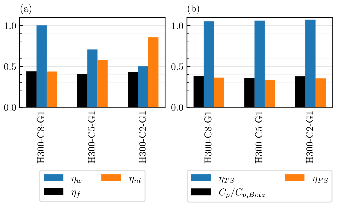
Figure 14 Comparison of wind farm performance for cases H300-C8-G1, H300-C5-G1, and H300-C2-G1 using (a) wake efficiency η_w and non-local efficiency η_nl and (b) turbine-scale efficiency η_TS and farm-scale efficiency η_FS.

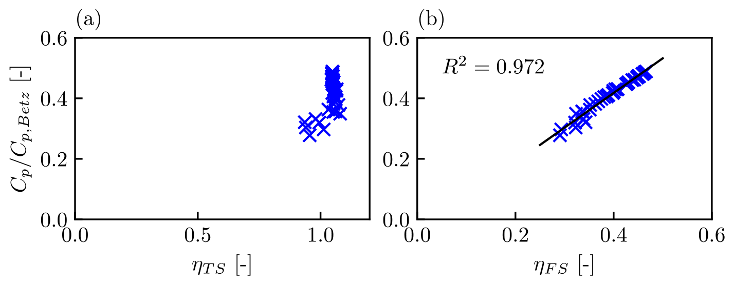
Figure 15 (a) Relationship between the overall farm efficiency $C_{\mathrm{p}}/C_{\mathrm{p},\mathrm{Betz}}$ and turbine-scale efficiency η_TS and (b) farm-scale efficiency η_FS, for all 38 LES cases with the dense staggered turbine layout. The R² value shows the coefficient of determination.

Figure 15 shows the values of η_TS and η_FS for the same staggered farm under 38 different atmospheric conditions. Almost all the variation in $C_{\mathrm{p}}/C_{\mathrm{p},\mathrm{Betz}}$ is explained by η_FS. This reflects the physical observation that different stratifications affect the large-scale farm–atmosphere interaction, changing the power generation efficiency on the farm scale. The value of η_TS is nearly the same for most cases, with a value of approximately 1.05 (discussed later in this section). The six cases with a lower η_TS are all with the lowest-capping-inversion height of 150 m. These cases show a larger change in wind direction within the farm, changing the turbine-scale flow characteristics and thus η_TS.

Next, we examine how the impact of changing the turbine layout is captured by the new efficiency metrics for the three atmospheric conditions discussed earlier in Fig. 10. As can be seen from Fig. 16, changing the layout from “staggered” to “aligned” changes the value of η_TS from approximately 1.05 to just above 0.8 for all three cases. Given that in aligned cases the second row of turbines produces much less power than the first, it might appear that η_TS≈0.8 is fairly high. However, this is reasonable since the overall farm efficiency ($C_{\mathrm{P}}/C_{\mathrm{P},\mathrm{Betz}}$) decreases by about 23 % when the layout is changed from staggered to aligned for all three atmospheric conditions considered. The farm-scale efficiency η_FS is practically unchanged with turbine layout, but it does change with atmospheric conditions. Therefore, using η_TS and η_FS allows us to separate the effect of turbine layout from the effect of atmospheric conditions.

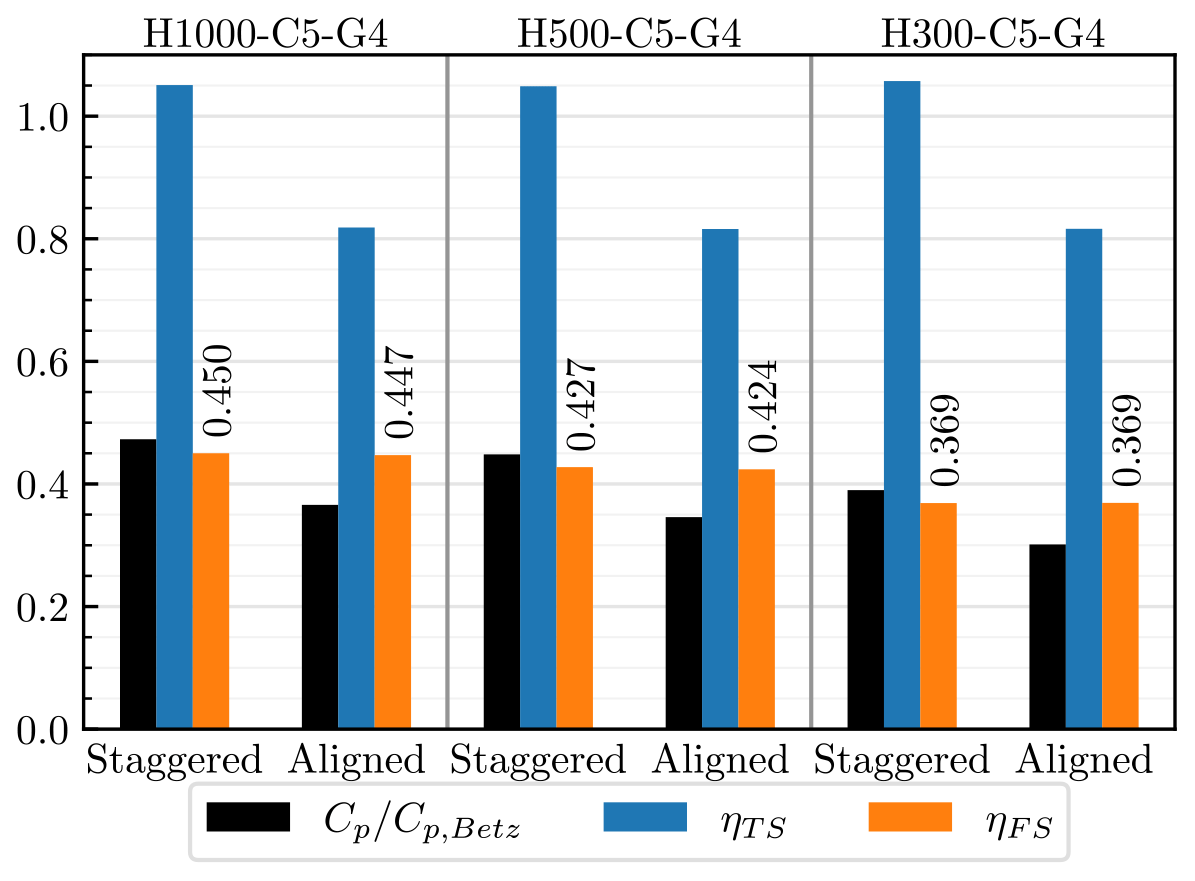
Figure 16 Comparison of farm performance for staggered and aligned turbine layouts in H1000-C5-G4, H500-C5-G4, and H300-C5-G4 atmospheric conditions, using the turbine-scale efficiency η_TS and farm-scale efficiency η_FS.

It is also worth noting that, for all these cases, the power losses are larger on the farm scale than on the turbine scale. Figure 16 shows that η_FS is smaller than η_TS for both staggered and aligned layouts despite the small turbine spacing (5 D) considered in these cases. This agrees qualitatively with the predictions made by Kirby et al. (2022).

The new efficiency metrics η_TS and η_FS are also applicable to smaller farms and larger turbine spacings. Here we simulated two additional layouts under the H500-C5-G4 atmospheric condition. In one case, half length, the streamwise length of the farm was halved to 6.93 km (shown in Fig. 17b). In the other case, double spacing, the turbine spacing was doubled in the x and y directions to 10 D×10 D (shown in Fig. 17c), whilst the farm size was kept constant. The results are compared with the standard case in Fig. 18, showing that the changes in overall farm efficiency are mostly due to changes in η_FS. The half-length case gives a higher η_FS because the farm-scale wind speed reduction is less severe for smaller wind farms (as discussed by Kirby et al. (2023b)). The double-spacing case gives an even higher η_FS because of the low array density, which reduces the total farm thrust compared to the standard case. The turbine-scale efficiency η_TS is similar and close to 1 for all three cases, reflecting the fact that turbine–wake interactions have limited impact on these staggered turbine arrays.

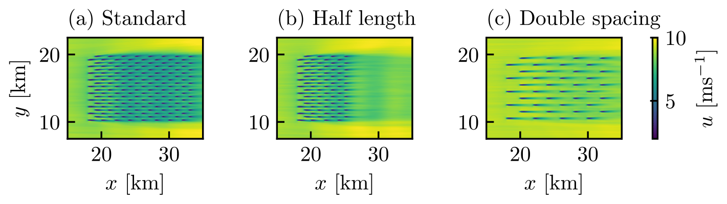
Figure 17 Time-averaged u velocity contours at the turbine hub height for the (a) standard turbine layout, (b) half length layout, and (c) double spacing layout.

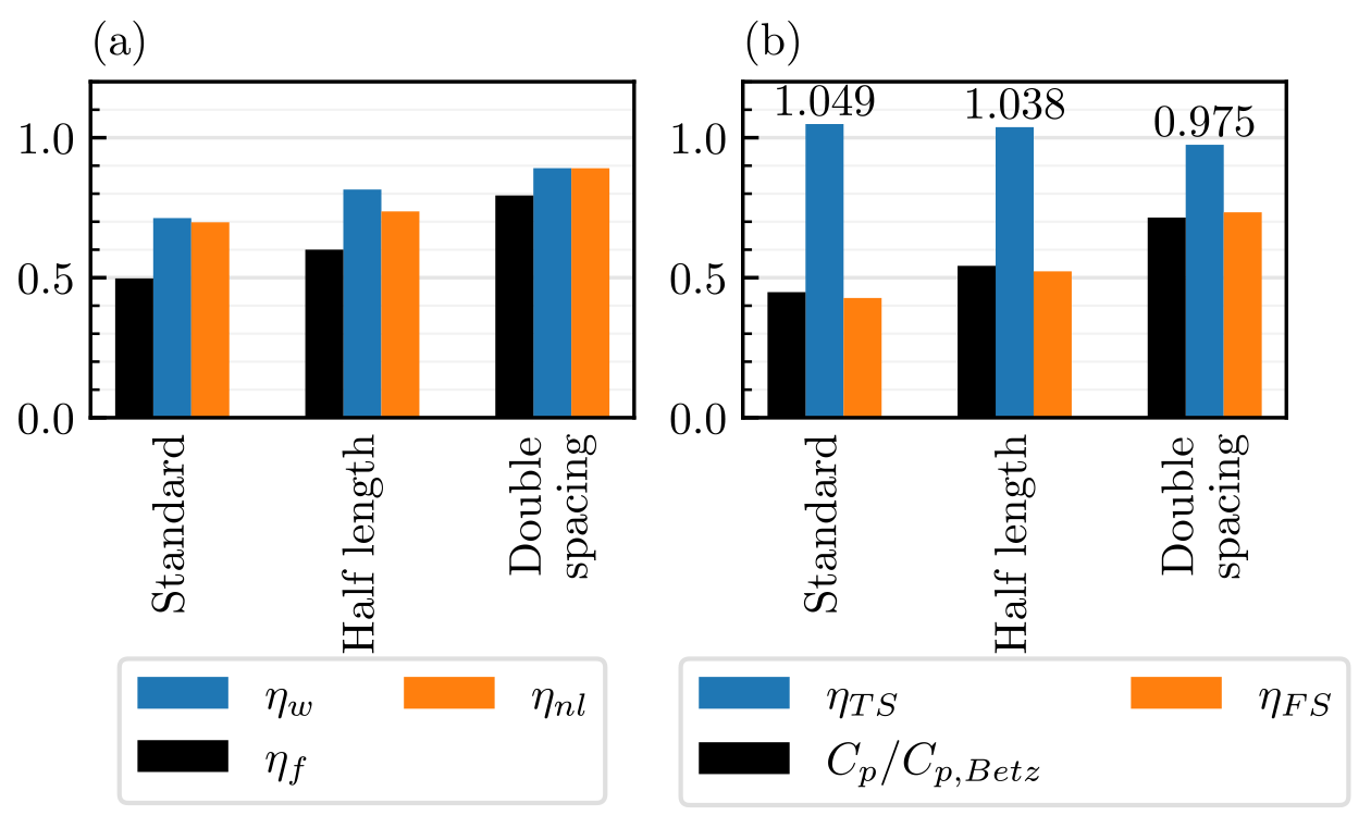
Figure 18 Comparison of farm performance for standard, half-length, and double spacing turbine layouts under H500-C5-G4 atmospheric conditions using (a) wake efficiency η_w and non-local efficiency η_nl and (b) turbine-scale efficiency η_TS and farm-scale efficiency η_FS.

It is worth noting that the staggered turbine layout with a 5 D×5 D spacing consistently gives η_TS of approximately 1.05 (see Figs. 15 and 18), meaning that, on the turbine-scale, the turbines are slightly more efficient at extracting power than isolated turbines. This is presumably due to the “local blockage” effect caused by neighbouring turbines (Ouro and Nishino, 2021; Nishino and Draper, 2015). It is important to note that η_TS=1 does not mean the maximum possible performance at the turbine scale. It means the performance, at the turbine scale, is equivalent to an isolated turbine that experiences the farm-average wind speed. The performance of an isolated turbine, for a given inflow speed, can be exceeded slightly due to local flow confinement effects. When the turbine spacing was doubled, η_TS was reduced to 0.975 (Fig. 18b). This suggests that the close turbine spacing caused η_TS to be greater than 1. Note that while a close lateral turbine spacing can increase η_TS slightly above 1, it also reduces η_FS, thereby reducing the overall farm efficiency $C_{\mathrm{p}}/C_{\mathrm{p},\mathrm{Betz}}$.

4.4 Analytical wind farm model

In this section we assess the ability of an analytical wind farm model (Kirby et al., 2023b) to predict η_FS. This analytical model predicts the farm-scale flows only and not the turbine–wake interactions. Hence, here we only compare the predictions of the farm-scale efficiency η_FS and not the turbine-scale efficiency η_TS. A summary of this farm model is shown in Fig. (19). Essentially, rather than using ζ_LES to calculate η_FS, here we predict η_FS using the expression

$$\begin{array}{}\text{(20)}& \mathit{\zeta }=\mathrm{1.18}+{\displaystyle \frac{\frac{\mathrm{2.18}}{C_{\mathrm{f}\mathrm{0}}}\frac{H_{\mathrm{F}}}{L}}{\mathrm{1}-\frac{{\mathit{\tau }}_{t\mathrm{0}}}{{\mathit{\tau }}_{\mathrm{w}\mathrm{0}}}}},\end{array}$$

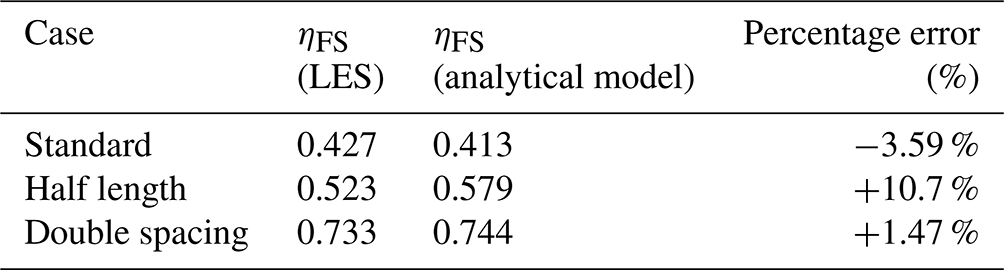
where L is the streamwise farm length, and τ_t0 is the undisturbed shear stress at a height H_F in the hub-height wind direction. Using this approach, we can predict η_FS instantly using only the undisturbed atmospheric conditions. It is important to note that this model (Eq. 20) currently only considers the impact of capping inversion height, and not capping inversion strength or free-atmosphere stratification. Figure 20a shows the distribution of percentage errors when predicting η_FS for the standard farm design with 29 atmospheric states (we excluded the lowest capping inversion cases “H150” where the capping inversion was below H_F), whereas Fig. 20b shows the relationship between the LES results and analytical predictions for these cases. The model gives good predictions of η_FS, with a mean absolute percentage error of 5.68 %. It is likely that the impact of free-atmospheric stratification, not considered in the current model, causes some spread and contributes to this error. There is a slight bias for underpredicting η_FS but the median percentage error is below 5 %. The prediction accuracy for the smaller farm and greater turbine spacing cases are also summarised in Table 5, showing that this first-order model gives satisfactory predictions for these cases as well.

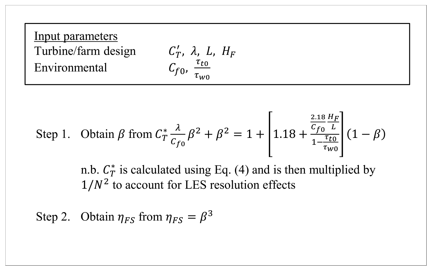
Figure 19 Input parameters and procedure used to calculate η_FS from the analytical model (Kirby et al., 2023b). Note that the analytical model itself is not dependent on the correction factor N. The reason why the correction factor is applied in step 1 is that, in order to make a fair comparison between the analytical model prediction and the LES, we need to account for the fact that the actual turbine thrust in the present LES (which does not include the correction factor during the simulation) is slightly higher than it should be.

Figure 20 Comparison of farm-scale efficiency η_FS obtained from LES and analytical predictions (Kirby et al., 2023b) for 29 standard cases: (a) box plot showing the distribution of prediction percentage errors and (b) relationship between the LES results and analytical predictions, with the R² value showing the coefficient of determination.

Table 5 LES and analytical model predictions of η_FS for standard, half length and double spacing layouts under H500-C5-G4 atmospheric conditions.

5 Discussion

Power losses for downstream rows of turbines in a wind farm (relative to the first row) are commonly attributed to turbine–wake interactions. For large farms, the downstream power losses are also affected by the atmospheric response, but it has been a challenge to model this effect accurately. In this study our LES results showed that, for a large staggered array of 160 turbines, the downstream power degradation was not due to turbine–wake interactions; i.e. individual turbine wakes (or more specifically, local flow regions having a lower flow speed than the average flow speed) were not directly causing the reduction in downstream turbine power.

It is worth noting that Porté-Agel et al. (2013) used LESs to show that turbine wake effects could reduce farm power by up to 35 % by simulating different wind directions; however, this power loss was calculated relative to the optimal wind direction (and not relative to the power of front-row turbines or isolated turbines). Furthermore, the wind farm simulated by Porté-Agel et al. (2013) was less than 20 % the size of the standard farm considered in this study. A recent study by Kirby et al. (2022) suggests that the relative importance of power losses due to turbine–wake interactions decreases with increasing farm size. The present study further supports the argument that farm-scale flow effects could play a leading role in power losses for large offshore wind farms.

Our LES results also showed that there was only a weak relationship between the farm blockage loss and the overall farm efficiency. This was due to the strong negative correlation between the blockage loss (represented by η_nl) and the wake loss (represented by η_w). This suggests that farm blockage, to a first order, acts to redistribute power across the farm rather than reduce the farm power. This has also been observed in the LESs performed by Lanzilao and Meyers (2022) and Stipa et al. (2024). The different stratifications changed the farm blockage, but the overall farm efficiency changed only slightly.

The turbine-scale efficiency η_TS and farm-scale efficiency η_FS are useful new metrics for understanding wind farm performance. They allow the impacts of turbine layout and farm–atmosphere interaction to be assessed separately. The farm-scale efficiency η_FS is insensitive to the turbine layout, and so the losses due to the atmospheric interaction can be predicted even before the turbine layout is decided. It is worth noting that, although actuator discs (or ideal turbines) were considered in this study, the new metrics η_FS and η_TS can be applied to wind farms with real (non-ideal) turbines as well. When the turbines are non-ideal, the power loss due to turbine design (relative to the power of ideal actuator discs) will reduce η_TS (as C_p in Eq. (13) decreases) but not η_FS.

For all turbine layouts and atmospheric conditions considered in this study, η_FS was lower than η_TS. This means that more power is lost due to the farm–atmosphere interaction than due to turbine–wake interactions. This was true even for the large farms with an aligned layout and close turbine spacing, where η_TS was about 0.8, whilst η_FS was less than 0.5. All staggered cases gave η_TS close to 1, suggesting no negative turbine–wake interactions. These results suggest the importance of focusing more on the modelling of η_FS (or the modelling of wind extractability factor ζ) in future studies of large wind farms.

In this study the assumption of two-scale separation was shown to be valid for large finite wind farms. This means that the modelling of large wind farms could be split into the modelling of turbine–wake interactions and the modelling of farm–atmosphere interactions, as suggested originally by Nishino and Dunstan (2020). It should be noted, however, that the present LES results are still for an idealised wind farm situation, i.e. quasi-steady situation with a horizontally homogeneous atmosphere. We found that the wind extractability factor ζ was insensitive to the internal or turbine-scale flow conditions (i.e. turbine layout and spacing). However, there may still be ways to manipulate the turbine-scale flows to increase ζ and, hence, the overall farm efficiency. One way could be to introduce some medium-scale unsteadiness by varying turbine operating conditions in time and thereby increase momentum entrainment into the farm (e.g. Goit and Meyers, 2015).

Another limitation of the present study is that we relied on a single LES dataset. In this study we focused mostly on a large and relatively dense wind farm. To test the applicability to a wider range of wind farm situations, future work can apply the new concepts of η_TS and η_FS to various wind farm LESs with different flow conditions (e.g. Baas et al., 2023). Future work could also work on validating the proposed models against wind farm SCADA data. The environmental input parameters (C_f0 and ${\mathit{\tau }}_{t\mathrm{0}}/{\mathit{\tau }}_{\mathrm{w}\mathrm{0}}$) could be calculated using ERA5 data. Data on the surface shear stress and boundary layer height from ERA5 could be used to estimate the shear stress ratio ${\mathit{\tau }}_{t\mathrm{0}}/{\mathit{\tau }}_{\mathrm{w}\mathrm{0}}$.

Future work should also focus on improving the analytical model of the momentum availability factor M and the wind extractability factor ζ (Kirby et al., 2023b). One improvement could be to explicitly model the impact of gravity waves on the farm pressure field (e.g. Smith, 2024). It will also be useful to improve the modelling of turbine-scale flows. Kirby et al. (2023a) developed a statistical model from LES data to predict $C_{\mathrm{T}}^{*}$ as a function of turbine layout for a fixed $C_{\mathrm{T}}^{\prime }$ value of 1.33. Future work can extend this data-driven approach to other turbine operating conditions.

6 Conclusions

In this study we analysed a large LES suite of wind farms in CNBLs. For all 38 simulation cases with the same staggered turbine layout, the overall farm efficiency η_f was not well correlated with the wake efficiency η_w (often referred to as normalised power) or with the non-local efficiency η_nl (representing farm blockage effects). Identical turbine layouts with different atmospheric stratifications (above the turbines) were found to give significantly different η_w values, which could not be explained by changes in effective turbine layout (due to changes in local wind direction) or changes in the rate of wake recovery. These results suggest that farm-scale flow effects could play a leading role in power losses in large wind farms.

The assumption of two-scale separation (Nishino and Dunstan, 2020) was evaluated in this study, using finite-size wind farm LES for the first time. The internal parameter $C_{\mathrm{T}}^{*}$ was found to be insensitive to external atmospheric conditions, whereas the external parameter ζ was shown to be insensitive to the turbine layout. Therefore, the assumption of two-scale separation seems valid for large offshore wind farms, at least under the ideal “quasi-steady” situation considered in this study.

Building upon the two-scale momentum theory, we have proposed new metrics of wind farm efficiency. The turbine-scale efficiency η_TS represents power losses due to internal turbine–wake interactions. The farm-scale efficiency η_FS reflects the losses due to the farm–atmosphere interaction. As can be expected from the two-scale separation observed, the new metrics seem very useful for understanding the aerodynamic performance of large wind farms. For all turbine layouts simulated, η_FS was found to be much lower than η_TS. This means that farm-scale flows have a greater impact on the overall farm efficiency than turbine-scale flows do. The analytical model developed recently by Kirby et al. (2023b) was shown to predict η_FS with an average error of 5.68 % from the LES results. Further developments in the modelling of farm-scale efficiency η_FS will be crucial in future studies of large wind farms.