Sensor-error-robust normal-behavior modeling for wind turbine drive train failure prediction using a masked autoencoder

Condition monitoring and failure prediction in wind turbines have become an increasingly important research area due to their substantial economic impact. Accurate early detection of developing faults enables more efficient maintenance planning and minimizes costly downtime. However, predicting failures from operational wind farm data remains challenging. Real-world datasets are often affected by measurement noise, incomplete expert knowledge, and extraneous operating conditions, all of which complicate the identification and classification of emerging problems. This work presents a methodology designed to address one critical obstacle: measurement errors caused by faulty or unreliable sensors. Such errors can substantially degrade the performance of normal-behavior models (NBMs), thereby hindering the detection of anomalies and incipient failures. To mitigate this issue, we introduce an approach based on masked autoencoders (MAEs) that selectively suppresses signals deemed unreliable by domain experts or automated diagnostics. The proposed method is evaluated using four datasets from real operational wind farms. We analyze the impact of sensor-induced errors on NBM performance and demonstrate how the MAE framework improves robustness in the presence of corrupted measurements. Furthermore, it is shown that the methodology achieves a high failure prediction accuracy even in contexts with substantial numbers of sensor errors. The results highlight the potential of the method to improve the accuracy of data-driven failure prediction systems in practical wind turbine drive train applications.

1 Introduction

The wind energy sector has expanded rapidly in recent years, driven by substantial investments and ambitious renewable energy targets. In 2024, Europe installed 16.4 GW (gigawatt) of new wind power capacity, including 12.9 GW within the European Union, bringing the total installed capacity of the continent to 285 GW. Onshore installations accounted for 84 % of this new capacity. Projections indicate that Europe will add approximately 31 GW of new wind capacity annually between 2025 and 2030, of which 23 GW is expected within the EU, resulting in a total installed capacity of roughly 351 GW by 2030 (Costanzo et al., 2025). These figures underscore the central and enduring role of wind power in the European energy system, and they highlight the significant economic importance of reducing the cost of wind energy.

Operation and maintenance (O&M) expenditures constitute a substantial share of the levelized cost of energy (LCOE) for wind turbines. For onshore turbines in the United States, O&M costs represent approximately 25 % of the total LCOE (USD 42 per megawatt hour (MWh)). For offshore fixed-bottom turbines, the share increases to 26.9 % (USD 117 per MWh), while for floating offshore turbines it is 17.8 % (USD 181 per MWh), the latter percentage being lower due to the larger proportion of capital expenditure in the total cost (Stehly et al., 2024). These values make it clear that reducing O&M costs is critical for further lowering the cost of wind energy.

A key strategy for reducing O&M expenditures is improving maintenance planning through reliable failure prediction. By identifying component degradation early, operators can schedule interventions more efficiently and avoid costly unplanned downtime. As a result, failure prediction and condition monitoring have become active research areas, employing a wide range of modeling approaches and data sources (Kestel et al., 2025). However, accurate prediction remains challenging due to data quality issues, incomplete expert knowledge, and the scarcity of failure examples.

Supervisory control and data acquisition (SCADA) data are especially valuable for condition monitoring (CM) and failure prediction because they are typically generated by default and do not require the installation of additional sensors. However, working with SCADA data also presents certain challenges. This paper addresses one specific but impactful data quality issue: sensor errors. Data-driven monitoring methods are highly sensitive to corrupted measurements, and sensor failures can degrade model performance from mildly inaccurate to entirely unreliable. For example, in normal-behavior models (NBMs), a single distorted input signal can propagate errors through the model and significantly compromise anomaly detection. To mitigate this problem, we propose a methodology based on masked autoencoders (MAEs) that enables selective deactivation of unreliable sensor signals while retaining the use of the full model without the need to train multiple parallel models.

The proposed approach is validated using data from four operational wind farms. The sensor failures investigated are real, not artificially generated. Through collaboration with industry experts, several characteristic sensor failure patterns were identified. The component failures used for the validation are all related to the drive train, i.e., gearbox and generator. They were identified by industrial partners at the moment of occurrence and through post hoc inspection of the component. The validation assesses the effectiveness of the masking strategy using multiple performance metrics, evaluates the capability of the model as an NBM, and analyzes the impact of masking on model stability.

2 Related work

2.1 SCADA-based condition monitoring of wind turbines

CM of wind turbines has emerged as a rapidly expanding research field, encompassing a wide range of methodological approaches. Based on the primary source of information, CM techniques can be categorized into three main groups: (i) SCADA-based approaches, which rely on readily available low-frequency data from the SCADA system of the wind turbine; (ii) vibration-based approaches, which utilize high-frequency signals collected from dedicated accelerometers; and (iii) acoustic emission-based approaches, which analyze high-frequency acoustic signals generated by turbine components (Kestel et al., 2025). Each category exhibits distinct advantages and limitations and addresses specific needs within the CM domain.

This paper focuses on SCADA-based CM methods that exploit low-frequency operational data. The most commonly used temporal resolution for SCADA data is 10 min, although higher sampling frequencies have also been reported in the literature (Chesterman et al., 2023). Within the SCADA-based paradigm, Wang et al. (2026) distinguish between physical-model-based approaches, which rely on explicit representations of turbine dynamics, and data-driven approaches, in which models are learned directly from historical SCADA data. This paper adopts the data-driven approach.

Data-driven CM encompasses a broad spectrum of methodologies. According to Wang et al. (2026), these methods can be divided into traditional data-driven techniques (e.g., trending analysis, statistical methods, and state–curve modeling) and machine-learning- and deep-learning-based approaches, including supervised, semi-supervised, and unsupervised methods. An alternative taxonomy is proposed by Tautz-Weinert and Watson (2017), who identify NBM, trending, clustering, damage modeling, alarm assessment, and expert systems as distinct categories. Comprehensive reviews of recent advances in wind turbine CM are provided in Wang et al. (2026), Kestel et al. (2025), Black et al. (2021), and Chatterjee and Dethlefs (2021).

This paper adopts the NBM approach, which has demonstrated strong performance in wind turbine health monitoring. A key advantage of NBM methods is that they learn a representation of normal system behavior that can be used for prediction and anomaly detection. NBM techniques can themselves be subdivided into several groups, with statistical methods, shallow machine learning models, and deep learning architectures being the most prominent (see Kestel et al., 2025, for an extensive overview).

The statistical group includes conventional modeling and dimensionality-reduction techniques, such as ordinary least squares regression (OLS) (Chesterman et al., 2022), principal component analysis (PCA) (Campoverde et al., 2022), and cointegration analysis (Dao, 2023).

Shallow machine learning models comprise widely used algorithms that are more flexible than statistical methods, particularly for capturing nonlinear relationships. Examples applied in wind turbine CM include random forests (RFs) (Turnbull et al., 2021), gradient boosting machines (GBMs) (Maron et al., 2022), and support vector machines (SVMs) (Castellani et al., 2021). While these models can achieve higher predictive accuracy, they typically require larger training datasets and offer reduced interpretability compared to statistical approaches.

Deep learning models represent the most recent and rapidly expanding class of NBM techniques. These methods rely on neural network architectures with multiple layers and have been applied extensively in modern CM systems. Common examples include deep neural networks (Verma et al., 2022), convolutional neural networks (CNNs) (Bermúdez et al., 2022), long short-term memory networks (LSTMs) (Trizoglou et al., 2021), and autoencoders (AEs) (Lee et al., 2024).

2.2 Sensor errors

This work addresses failure prediction in the presence of sensor errors, which are conditions under which corrupted sensor signals can significantly degrade predictive performance. Following the ISO definition, a measurement error is the difference between the measured value and the true value of the measurand and can generally be decomposed into random and systematic components (BIPM et al., 2008). We define a sensor error as any condition causing a sensor to produce such measurement errors. In a similar vein, Balaban et al. (2009) describe a sensor error or fault as an unexpected deviation in the observed signal in the absence of any underlying anomalous system behavior.

A wide variety of sensor fault modes has been reported in the literature, and several taxonomies have been proposed. Balaban et al. (2009) identify the following major categories:

• Bias is a constant offset from the nominal signal, often caused by miscalibration or physical changes in the sensing element (e.g., a temperature sensor consistently overestimating by 10 °C).

• Drift is a time-varying offset from nominal behavior.

• Scaling involves multiplicative distortion of the signal magnitude while preserving waveform shape.

• Noise is the random fluctuations superimposed on the true signal.

• Hard faults occur when the signal becomes fixed at a particular value, including complete signal loss or a “stuck” sensor.

An alternative but partially overlapping taxonomy is provided by Teh et al. (2020), who introduce an additional outlier category representing abrupt, unstructured deviations beyond expected thresholds. They also identify specific subtypes such as “stuck at zero”, which is a sub-category of the hard-fault class described in Balaban et al. (2009).

In practice, data acquired from complex industrial systems often contain multiple fault types simultaneously. This complicates downstream analysis, as some faults, such as bias, may be subtle and not visually apparent. Their detection typically requires models that capture relationships across multiple sensor signals. A wide range of such models has been explored. Two common strategies are data imputation and data fusion. Teh et al. (2020) review imputation methods for handling missing or noisy data, including association rule mining (ARM), clustering, k-nearest neighbors (KNNs), singular value decomposition (SVD), and various hybrid techniques. Approaches for denoising include empirical mode decomposition, Savitzky–Golay filtering, and multivariate thresholding. A broader survey is provided by Trapani and Longo (2023), who group existing methods into categories such as machine learning, statistical techniques, PCA, Kalman filtering, SVM, digital twins, Markov models, fault-tree analysis, and others.

The low temporal resolution of SCADA data, combined with the often prolonged persistence of sensor faults (see the Methodology section), renders sensor errors a particularly critical issue for failure prediction in wind turbines using SCADA-based NBMs. Sensor faults in SCADA systems can lead to extended periods of unreliable or unusable data. Consequently, such faults can result in months of invalid NBM predictions, substantially reducing the practical value of the analysis. For this reason, the development of sensor-error-robust NBM models is of significant importance.

2.3 Masked autoencoder

Masked machine learning models form a prominent class of self-supervised learners. Their initial development was driven by natural language processing (NLP), with Bidirectional Encoder Representations from Transformers (BERT) being a well-known example. BERT employs a masked language modeling (MLM) objective, in which parts of the input sequence are masked and subsequently predicted during training (Devlin et al., 2019).

MAEs have since been adopted in computer vision. For instance, He et al. (2021) introduce an MAE method for image data based on an asymmetric encoder–decoder architecture. This design differs from ours, which employs a strictly symmetric architecture. Their approach also uses a substantially higher masking ratio (75 %), whereas the ratio in our study is considerably lower. Additionally, the data modality (images versus the tabular data used here) introduces fundamental differences in model structure and learning dynamics. Several other works have extended MAE to computer vision tasks (Chen et al., 2024; Madan et al., 2024).

In contrast to vision-focused research, our work applies MAE to tabular sensor data, which requires important algorithmic modifications. Several recent papers have investigated this direction. Du et al. (2023) use MAE for missing-value imputation in tabular datasets. Similarly, Kim et al. (2025) develop a proportional masking strategy designed to compensate for biases that arise with naive random masking and demonstrate that multi-layer perceptron (MLP)-mixed models often outperform transformer-based alternatives for tabular data. A general masked encoding methodology for tabular data is presented in Majmundar et al. (2022), with further specialization for time-series applications explored by Li et al. (2023), who use masking to learn stronger temporal representations.

To our knowledge, the methodology most closely related to the one proposed in this paper is that of Fu and Yan (2024), who apply an MAE to streamline the fault detection, isolation, and accommodation (FDIA) pipeline for offshore wind turbines. Despite the conceptual similarity, several important differences remain. First, their AE topology does not include a bottleneck layer, whereas our method explicitly enforces one, and they do not incorporate a feature expansion layer. Their training noise level is also substantially lower (maximum 0.2) compared with ours (0.5). In terms of input structure, they use only masked SCADA data, while we provide both masked SCADA data and an explicit masking matrix. Their validation focuses on blade bending moments with simulated sensor faults, whereas our study evaluates generator and gearbox temperature sensors that exhibit real sensor failures. Furthermore, we additionally assess the ability of the model to detect wind turbine component failures, while Fu and Yan (2024) concentrate solely on sensor fault detection. As a result, the methodology developed in this paper is tailored to component failure prediction under realistic sensor fault conditions, aligning more closely with operational needs.

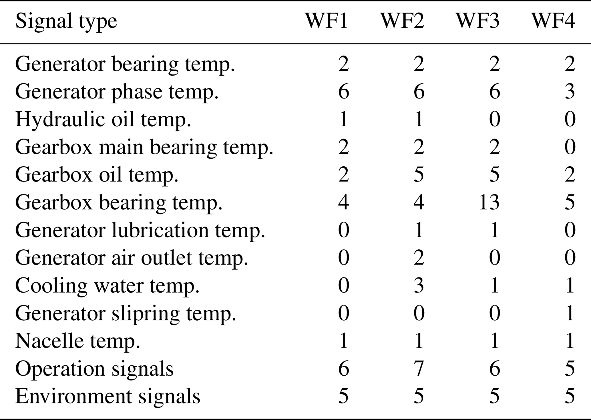
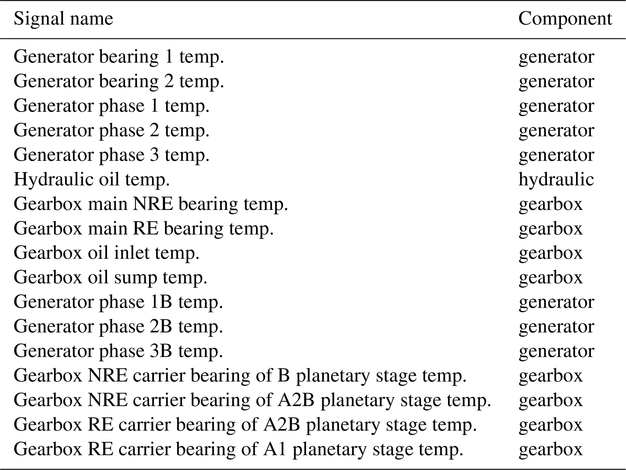
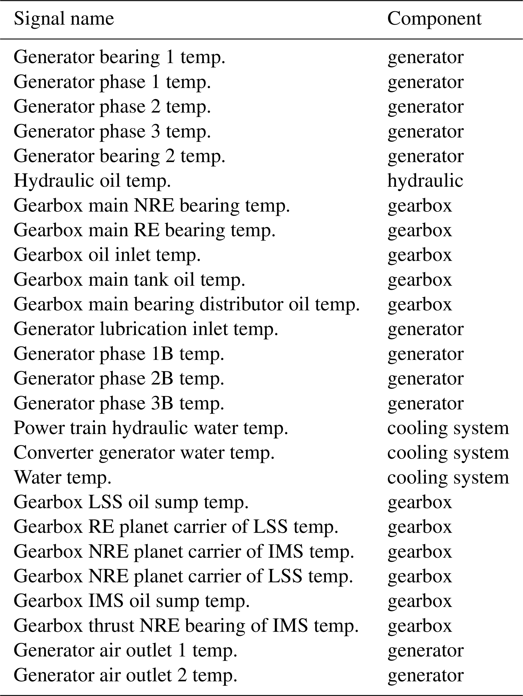
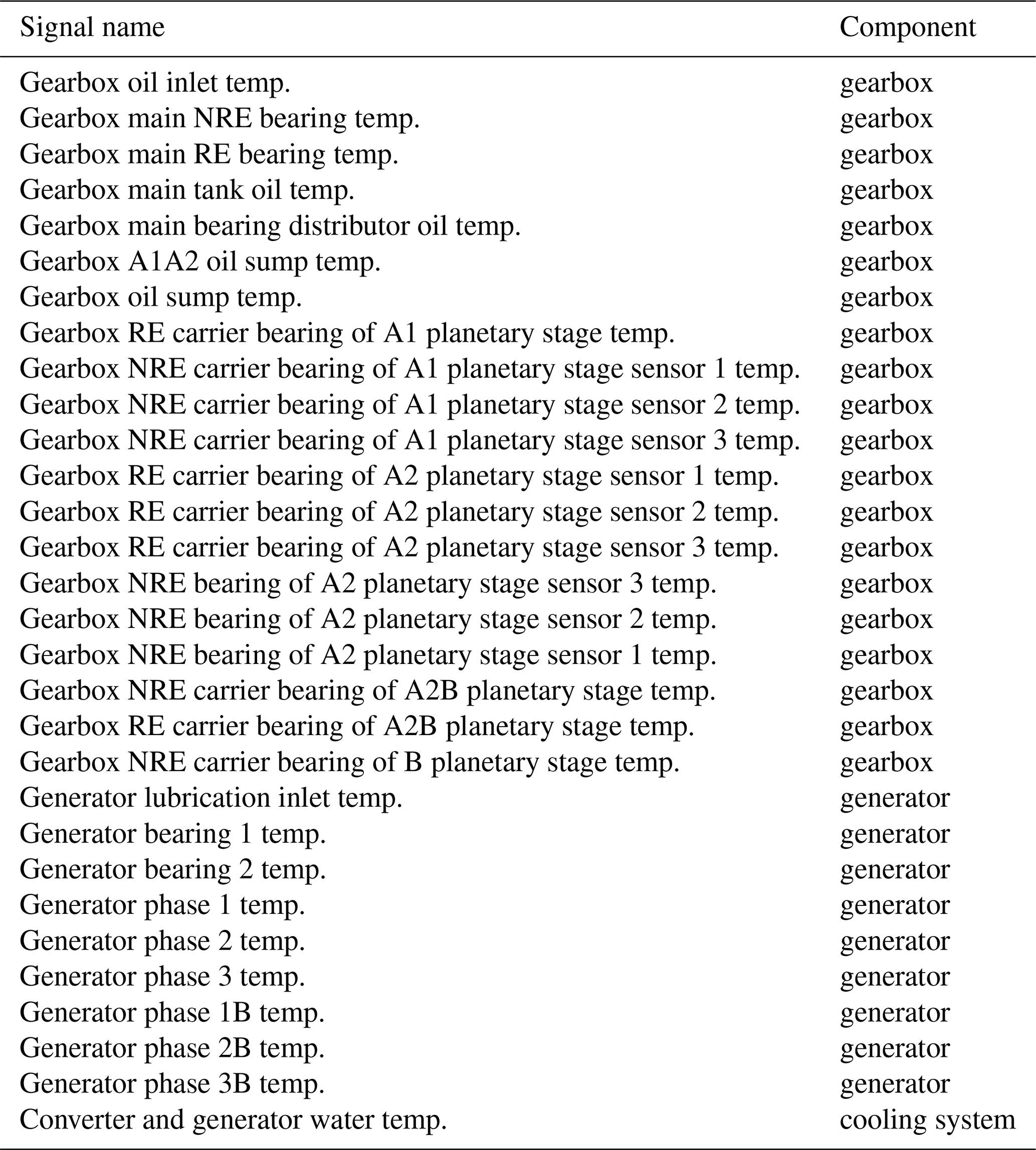
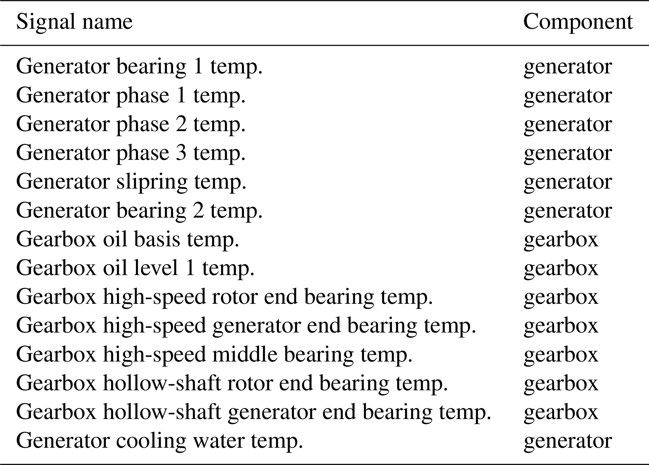
Table 1 High-level overview of signals used by the NBM for the different wind farms.

3 Methodology

3.1 Input data

This study uses 10 min SCADA data from four operational offshore wind farms (WF1–WF4). The dataset spans three wind turbine types with rated capacities between 3 MW (megawatt) and 10 MW. Across the four wind farms, 136 turbines are included, representing an aggregated observation period of approximately 1000 turbine years. The SCADA data provide measurements of component temperatures and environmental and operational conditions. Only a subset of these signals is used in this work. Table 1 provides an aggregated overview, with detailed signal lists presented in Tables A1, A2, A3, and A4. The primary focus of this research is on detecting abnormal behavior in temperature-related signals under the condition that sensor errors can occur. These anomalies may serve as precursors to component failures.

3.2 Data preprocessing

Because anomaly detection and failure prediction for wind turbines must rely on operational SCADA data, which frequently contain gaps, sensor issues, and other imperfections, several preprocessing steps are required before model development. The following steps summarize the procedure adopted in this study:

• Data aggregation. The original 10 min SCADA data are aggregated to a 1 h resolution. This reduction in temporal resolution is acceptable because the degradation mechanisms of interest evolve over long timescales (days to months). Aggregation also reduces high-frequency noise, resulting in cleaner input for model training.

• Major failure identification. Major wind turbine failure events are identified in the data and stored in a list for later use. A major failure is defined as a turbine downtime exceeding 7 d. Such prolonged outages typically indicate the failure of a major component requiring replacement. Given the size of these components and the logistical constraints associated with offshore maintenance, replacement can be time-consuming. Identifying major failures is essential, as post-replacement behavior (particularly temperature profiles) may differ from pre-failure behavior and may therefore require recalibration. In practice, this means that if a turbine is offline for more than 7 d, it is registered as an event in a list. Each event is characterized by the turbine ID and the start and end times of the offline period.

• Healthy and unhealthy data identification. Data generated by wind turbines that are unhealthy are identified; the remaining data are considered healthy. The challenge is however that SCADA data are unlabeled and thus do not explicitly indicate whether the turbine is operating in a healthy state. For training an NBM, it is important to use data that reflect healthy operation as closely as possible. A pragmatic assumption is adopted: data occurring within 90 d prior to a major failure, or within 5 d after it, are considered unhealthy. All remaining data are treated as healthy.

• Train–validation–test split. The datasets are split into three parts, i.e., training, validation, and testing datasets. Training and validation data are drawn from a single 1-year window. By selecting 1 year of data, the data include all seasons. This is important as seasonal variability in SCADA signals tends to influence model output. The splitting of the window into training and validation is done according to the following principle: 80 % of the observations are assigned to the training dataset and 20 % to the validation dataset. All remaining data outside this 1-year window form the test set.

• Measurement error handling. Measurement errors are removed from the training and validation datasets. Sensor failures occasionally occur in operational SCADA systems, producing unreliable measurements. To prevent such corrupt data from influencing model training, measurement errors are identified and removed (as well as possible) from the training and validation datasets using expert-defined thresholds. Measurement errors are not removed from the test dataset.

• Missing value handling. Observations with missing values are removed. Missing values in SCADA data typically arise from sensor malfunctions or communication interruptions. Neither mechanism is expected to depend on the underlying operational state, suggesting that the missingness mechanism is likely missing completely at random (MCAR). Under this assumption, the simplest and most transparent approach, i.e., removing observations containing at least one missing value, is applied.

• Feature engineering. Several additional features are derived to enhance model performance. These include (i) operating conditions following the IEC standard; (ii) wind vector components derived from wind speed and direction; (iii) nacelle-wind direction offset, which may indicate increased mechanical loading when large; and (iv) blade–angle differences (when available), as large offsets may also correspond to increased drive train stresses.

3.3 Normal-behavior modeling

A wide range of techniques for anomaly detection and failure prediction have been proposed in the literature, including trending approaches, clustering methods, NBMs, physics-based damage models, alarm-based systems, and expert-rule systems (Tautz-Weinert and Watson, 2017). In this work, we adopt the NBM approach, which is widely used and has demonstrated strong performance in industrial monitoring applications.

Normal-behavior modeling consists of two steps. First, a model is trained exclusively on data representing healthy system behavior. When successful, the model learns the normal relationships among the variables. In the second step, the model is applied to new data to generate predictions that represent the expected (healthy) behavior. Deviations between the predictions and the measured values are interpreted as indicators of abnormal or degraded operation: small deviations correspond to nominal behavior, whereas large deviations suggest emerging faults.

In this study, an MAE is employed as the NBM. This architecture is specifically chosen for its ability to handle measurement errors and missing values caused by sensor failures. By incorporating an explicit mask, the AE can learn normal inter-signal relationships even when some sensor values are unavailable or unreliable.

Figure 1 Schematic overview of the masked autoencoder methodology.

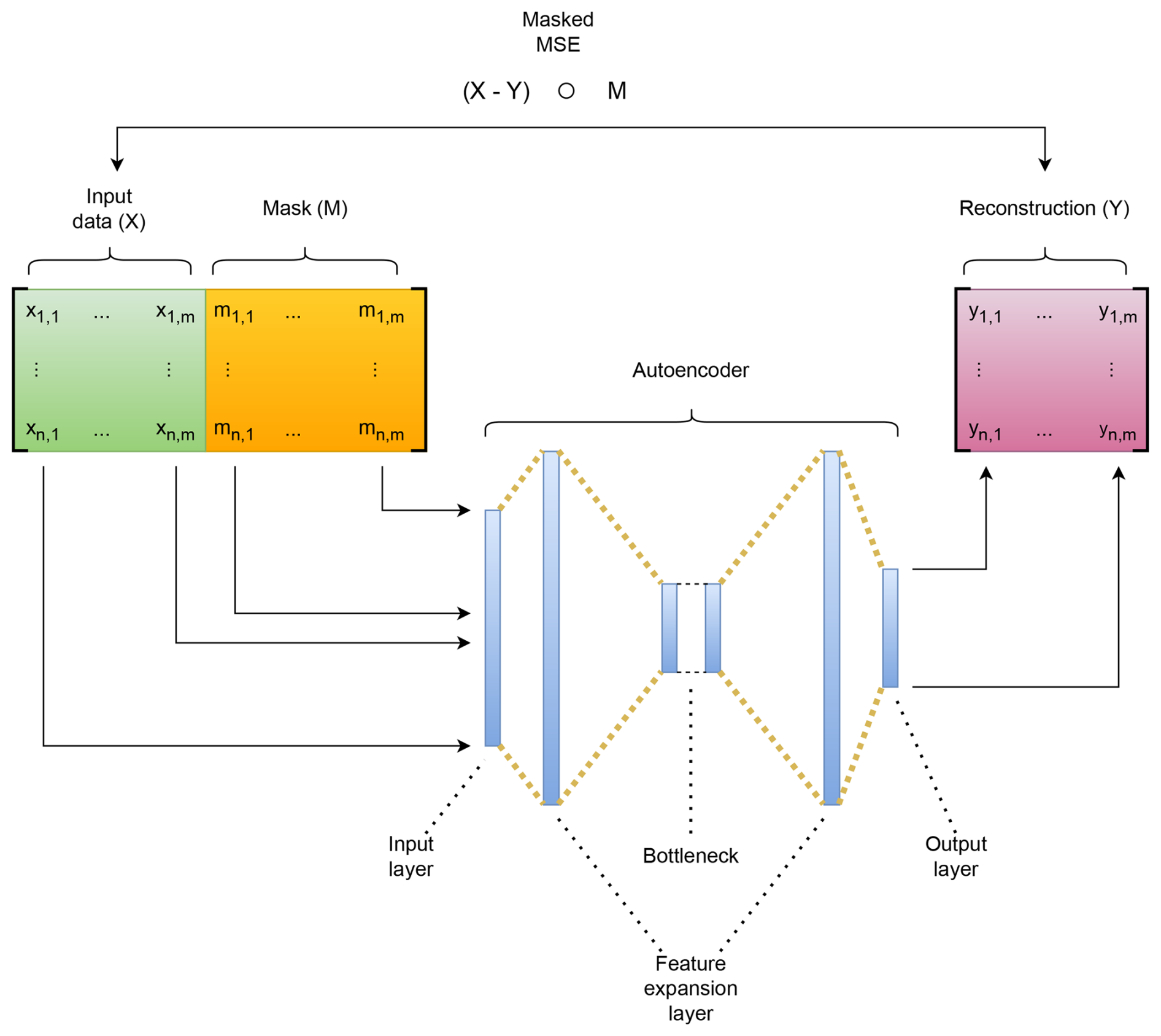
3.3.1 Masked autoencoder training and prediction

We develop a variant of an MAE tailored to the structure of SCADA data. Figure 1 gives a schematic overview. Let the input matrix X contain n observations and m features, where x_i,j denotes the value of feature j in observation i. Each value has an associated mask entry $m_{i,j}\in \mathit{\{}\mathrm{0},\mathrm{1}\mathit{\}}$, forming the mask matrix M. Here 0 indicates that the value in X is masked and 1 otherwise. If a value in X is masked, its value is changed to the masking value 0 ($m_{i,j}=\mathrm{0}\Rightarrow x_{i,j}=\mathrm{0})$. Before being fed into the AE, X and M are concatenated, enabling the network to distinguish between true zeros and masked entries without requiring out-of-range mask values. The AE comprises an encoder ($f_{\mathit{\theta }}:{\mathbb{R}}^{\mathrm{2}m}\to {\mathbb{R}}^d$) and a decoder ($g_{\mathit{\varphi }}:{\mathbb{R}}^d\to {\mathbb{R}}^m$), producing the reconstruction ${\mathit{Y}}_i=g_{\mathit{\varphi }}\left(f_{\mathit{\theta }}\right({\mathit{X}}_i,{\mathit{M}}_i\left)\right)$. Training minimizes a masked mean squared error (MSE) loss $l(\mathbf{Y},\mathbf{X},\mathbf{M})=\left|\right|(\mathbf{Y}-\mathbf{X})\odot \mathbf{M}\left|\right|$, ensuring that only unmasked elements contribute to the loss.

Model architecture and training parameters are optimized using the Keras Tuner Hyperband algorithm, which allocates computational resources via a multi-armed bandit strategy (Li et al., 2018). Separate training and validation sets are used to avoid overfitting. Several architectural constraints are imposed to limit the hyperparameter search space:

• Symmetric architecture. The encoder and decoder are mirror images, except that the encoder input layer has dimensionality 2m due to concatenation of X and M, while the decoder outputs m reconstructed features.

• Feature expansion layer. The first hidden layer of the encoder expands the dimensionality, with the number of units constrained to [2.5m,8m].

• Bottleneck layer. The latent dimension d is required to satisfy $d\in [\mathrm{0.25}m,\mathrm{0.75}m]$, ensuring a compressed representation.

• Intermediate layers. Units in intermediate layers follow an exponential decay pattern determined by the expansion-layer width 2m, the bottleneck width d, and the number of layers h between them: $r=(\frac{d}{\mathrm{2}m}{)}^{\frac{\mathrm{1}}{h}}$.

Training is capped at 200 epochs with early stopping (patience = 10). For MAE, it is important that candidate models are allowed sufficient training time before elimination. Accordingly, the Hyperband reduction factor is set to 2, slowing down the elimination schedule, and the hyperband_iterations parameter is set to 3 to encourage adequate exploration.

Table 2 Overview of the number of layers and number of units per layer for the best model for WF1, WF2, WF3, and WF4.

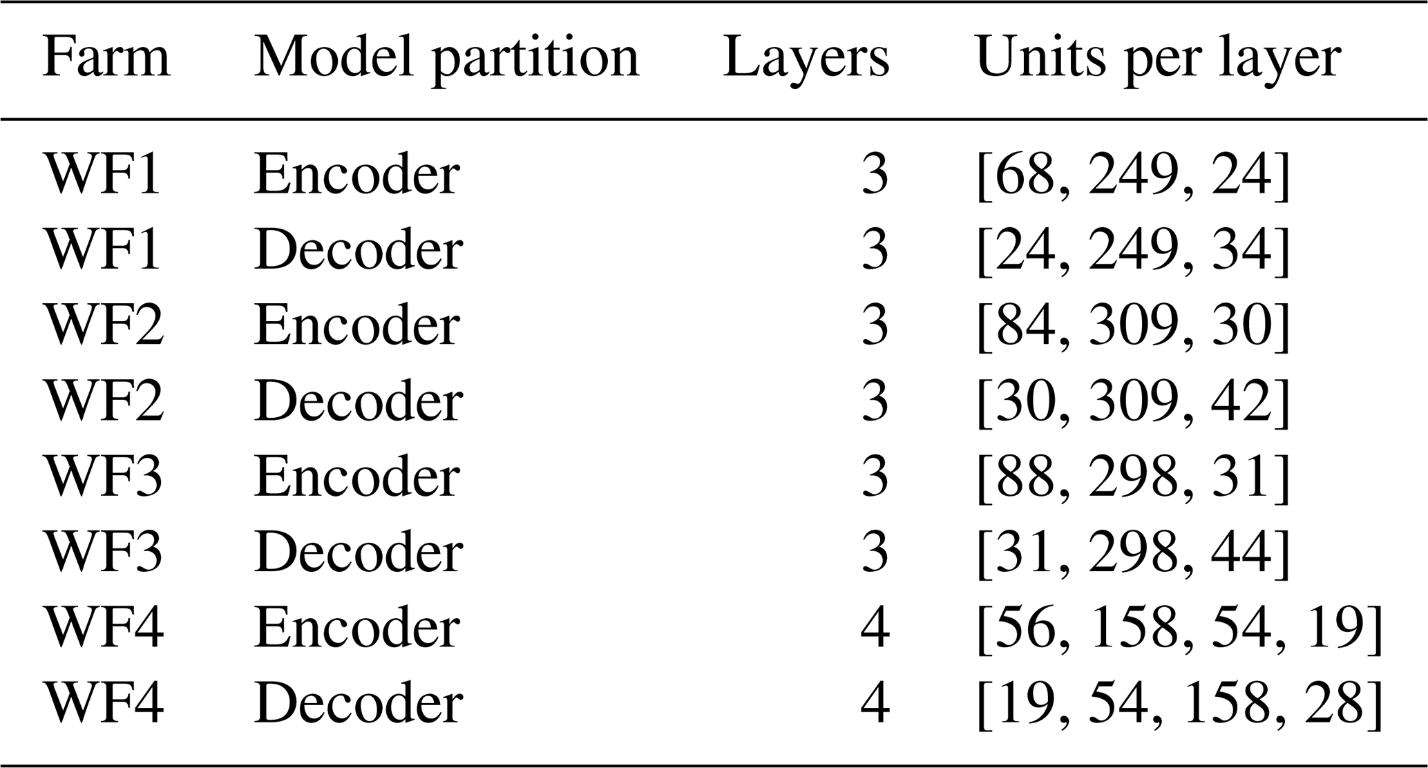
For three of the four datasets, the best models selected through hyperparameter tuning are MAE architectures whose encoders and decoders each comprise three layers. For the WF4 dataset, both the encoder and the decoder consist of four layers. In all cases, the bottleneck induces a substantial reduction in dimensionality. An overview of these architectures is provided in Table 2.

A single model provides only point estimates and does not quantify prediction variability. To obtain stability estimates, we apply bootstrapping (Efron, 1979). The training dataset is resampled with replacement 200 times, generating 200 datasets of equal size. Because the autoencoder relies on masking during training, a new random mask with a noise ratio of 0.5 is generated for each resampled dataset.

For each bootstrap sample, a model with the best-performing hyperparameters is trained from scratch with randomized weights, again for up to 200 epochs with early stopping. This procedure yields 200 independently trained AEs. During prediction, each model produces its own reconstruction errors, resulting in an ensemble of 200 reconstruction error time series that collectively characterize both expected behavior and predictive uncertainty.

3.3.2 Evaluation of the masked autoencoder

The bootstrapped models are used to generate predictions on the test data in two ways: first without masking measurement errors and then with masking applied. This enables an assessment of the impact of masking. When masking is applied, the mask for the affected signal(s) and the corresponding signal values are set to 0 for the relevant time window. This reflects a realistic operational scenario. The procedure is carried out for all sensor error cases described in Sect. 3.1. Three aspects of the methodology are evaluated: (i) the extent to which masking corrects the prediction artifacts caused by sensor failures, (ii) the accuracy of the model on healthy data, and (iii) the ability of the MAE to identify an approaching failure.

The three aspects are relevant for the following reasons. Methodologies that model the normal behavior of a target signal using other available signals as predictors are inherently sensitive to sensor errors affecting these predictors. If a predictor contains a sensor error and exhibits correlation with the target signal, the estimated normal (or healthy) values of the target may be distorted. This represents a major challenge in condition monitoring based on the NBM approach, as it can lead to a high number of false positives. If the MAE is able to temporarily suppress the influence of such faulty predictors, this issue can be mitigated. For this reason, investigating the first aspect is of particular importance.

The second aspect provides insight into the ability of the model to accurately approximate the original healthy data. Large reconstruction errors indicate that the model does not adequately capture the relationships among the different signals. For anomaly detection, this limitation is not necessarily critical, as the primary objective is to distinguish between healthy and unhealthy data (see aspect 3). However, in such cases, the model would have limited value as a predictive tool. Ideally, we have an NBM that models the healthy data well (small reconstruction error) and can distinguish healthy from unhealthy data easily.

The third aspect concerns the need to ensure that a solution capable of mitigating the impact of sensor errors remains effective in predicting component failures. This is, ultimately, the primary objective of the normal-behavior modeling approach in wind turbine condition monitoring. In principle, it is possible to design a model that is robust to sensor errors but performs poorly in failure prediction. A trivial example is a model that ignores all predictors (i.e., sets all predictor parameters to zero) and outputs a constant value. While such a model would be insensitive to sensor errors in the predictors, it would most likely be ineffective for condition monitoring under variable conditions. To ensure that this is not the case for the MAE, we additionally evaluate it with respect to its ability to predict component failures.

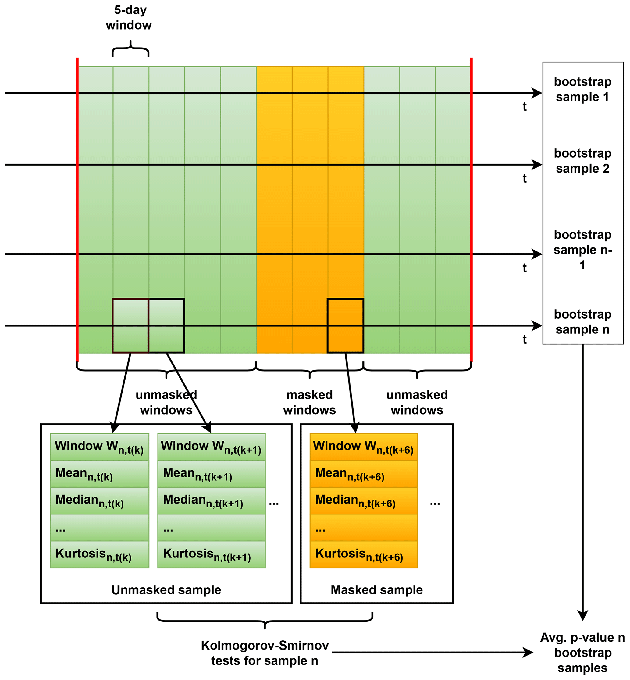
Figure 2 Schematic overview of the methodology used for determining the similarity between the reconstruction error distributions of masked data and nominal data.

The first aspect is assessed by comparing the reconstruction errors of each signal (except the one suffering from the sensor error) inside a masked window (meaning at least one signal is generated by a faulty sensor and is masked) to those outside the window. If the MAE functions correctly, these reconstruction errors should be statistically similar. The comparison is based on several distributional properties: mean, median, standard deviation (SD), interquartile range (IQR), skewness, and kurtosis. To ensure fair comparison, only data from the same inter-failure data window (IFDW), which is a continuous interval between two consecutive major component failures/replacements or between turbine commissioning and the first major failure, are used for each sensor error case. Since major replacements can substantially alter the relationships between signals, comparing reconstruction errors across different IFDWs would lead to misleading conclusions.

The IFDW data are segmented into blocks of 5 d, and the metrics listed above are computed for each block. Blocks are then labeled as masked or unmasked (masked if they are part of the masked window, unmasked if they are not). To determine whether the distributions differ between the two groups, the two-sided Kolmogorov–Smirnov test (KS test) (95 % significance level) is applied. For each signal and each bootstrapped model, one p value is obtained, yielding 200 p values per signal (one for each resampled dataset). Their mean is then computed. The MAE is considered to perform adequately if, for all signals except the one affected by the sensor error, the average p value exceeds 0.025 (2.5 %).

The procedure for testing whether the distributions are similar is based on multiple tests. For each sensor error case, six metrics are tested using a KS test. Based on these six tests, a decision can be taken on whether the distributions are similar or not. However, due to the fact that multiple tests are used, the p values should in principle be adjusted for multiple hypothesis tests. This is necessary for the following reason. If a hypothesis is tested at the 5 % significance level, then there is a 5 % chance of rejecting a true null hypothesis. If however six independent tests are done, this rejection chance becomes 26.49 %, which is substantially higher. There are several methods to compensate for this. One well-known method to control the family-wise error rate is the Bonferroni correction (Shaffer, 1995). Using this correction, to keep the Type I error rate at 5 %, the significance level should be divided by 6, which means 0.83 %. This method is however very conservative, which reduces the power of the test significantly.

Because the validation is conducted in operational rather than simulated or laboratory settings, uncontrolled variables may introduce unforeseen effects. Nevertheless, aside from minor discrepancies, the results for most signals should be robust and unambiguous. To make sure that the KS test has sufficient power, the IFDW must be sufficiently long and contain sufficient healthy data (not influenced by component damage). This condition will drive the selection of sensor error validation cases.

The second aspect is evaluated by computing the absolute and relative reconstruction errors for data classified as healthy. Healthy data are defined as observations that are not labeled as unhealthy, where unhealthy data correspond to observations occurring within 90 d prior to a major failure. For each signal of every turbine across the four wind farms, the absolute reconstruction error is calculated as the difference between the reconstructed signal and the original signal. The relative reconstruction error is defined as the ratio of the absolute reconstruction error to the original signal value. The absolute and relative reconstruction errors are subsequently averaged per component (i.e., gearbox and generator) for each wind farm. In addition, the corresponding SDs are computed.

The third aspect is evaluated by examining how well the model differentiates between healthy and unhealthy data using the abnormal-behavior sensitivity metric (ABSM). This is also based on IFDWs. This ensures that healthy and unhealthy data are both generated under consistent component configurations. Unhealthy data are defined as observations within 90 d preceding a major failure, which corresponds to the last 90 d of the IFDW; healthy data are defined as the first 30 d of the corresponding IFDW. For each signal, the ratio is computed between (i) the fraction of unhealthy observations for which the 2.5th percentile of the reconstruction error exceeds zero and (ii) the corresponding fraction for healthy observations.

Since the failure logs delivered by the industrial partners specify only whether a failure concerns the generator or the gearbox (and not which subcomponent has failed), the results are aggregated per component by taking the maximum ratio among all signals associated with that component. This approach reflects practical usage, where an analyst inspects multiple signals and determines which component shows the strongest deviation. For the method to be useful as an anomaly detector, this ratio should be substantially greater than 1, indicating clear differentiation between healthy and unhealthy behavior. A ratio above 2 is considered strong evidence, values between 1.25 and 2 indicate marginal identification, and values below 1.25 are classified as misses.

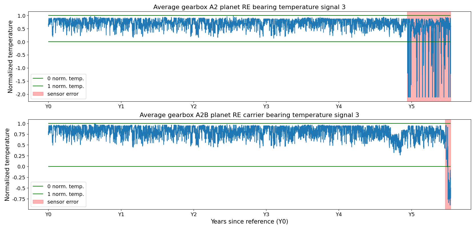
Figure 3 Sensor failures in two signals of the turbine in WF1. The sensor failure is a combination of types, i.e., bias and scaling.

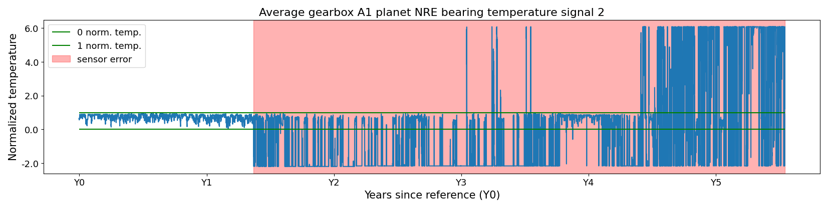
Figure 4 Sensor failure in the temperature signal of the turbine in WF3. The sensor failure is a combination of types, i.e., bias and scaling.

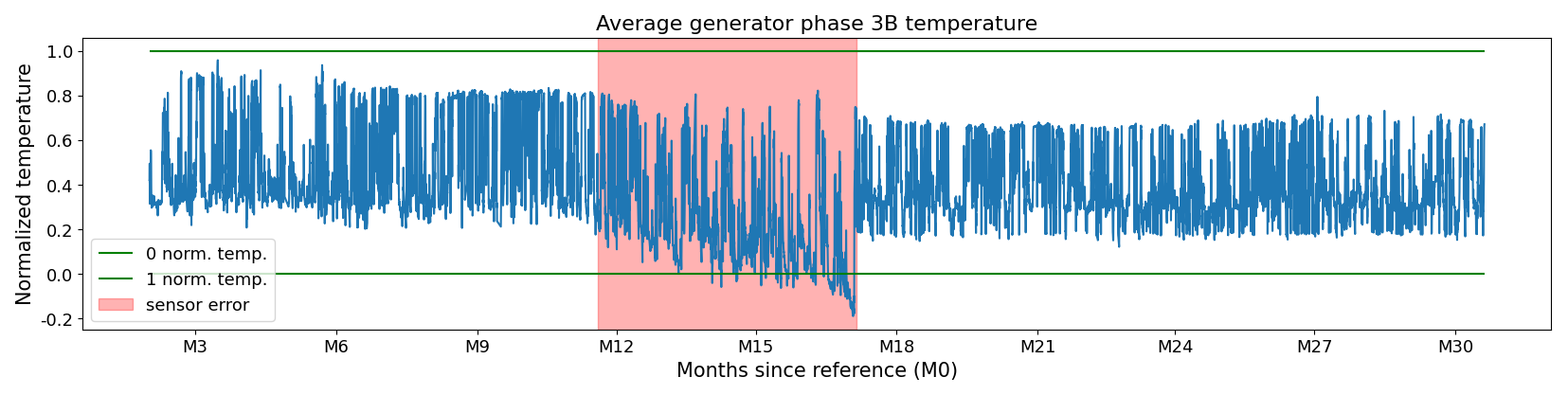
Figure 5 Sensor failure in the temperature signal of the turbine in WF2. The sensor failure is of the drift type.

3.4 Sensor errors

The input data contain numerous sensor failures that manifest as measurement errors. For validation, 12 cases were selected from WF1, WF2, and WF3. The selection is based on their suitability for the analysis. As explained in the previous section, the IFDW – of which the masked window is a part – must be sufficiently long and contain sufficient healthy data. A sufficient number of samples need to be available for the KS test. This implies that both the sensor error window and the healthy or normal data window surrounding the sensor error window must be large enough. This was the case for 12 cases.

The cases include several of the sensor failure types discussed in Sect. 2. Some sensor errors are readily identifiable because they produce physically impossible values, as illustrated in Figs. 3 and 4. These typically correspond to biased sensors or hard faults. Other errors are more subtle, arising from gradual sensor drift. This drift appears as a slow upward or downward trend and may only produce implausible values after an extended period, if at all (see Fig. 5). These cases are more difficult to detect, especially because temperature-related signals may also deviate due to legitimate causes, such as component wear or damage.

To make the identification of the sensor errors easier, the MAE was first applied in a non-masking mode, meaning that no observations or signals are switched off. In this configuration, sensor failures manifest as characteristic anomalies in the reconstruction errors. In some instances, the failures appear as isolated outliers, but more commonly they result in prolonged periods during which the reconstruction error deviates consistently from the expected pattern, reflecting biased readings or hard faults, as visible in Figs. 3, 4, and 5. These extended error periods arise because sensor issues are often not noticed immediately, and even once identified, repairs or replacements typically occur only during scheduled maintenance. In some cases, the sensor errors persist for several years before the issue is resolved (see Fig. 4). These patterns were identified (in collaboration with industrial partners) and logged (i.e., turbine, signal, start, and end). The log was then used to switch off signals during the run in masking mode.

The sensor errors occur across a broad range of sensors, including hydraulic oil temperature sensors, gearbox oil sump temperature sensors, gearbox A2B planet non-rotor-end (NRE) carrier bearing temperature sensors, gearbox A2B planet rotor-end (RE) carrier bearing temperature sensors, generator phase 3B temperature sensors, generator air outlet 1 temperature sensors, gearbox A1 planet NRE bearing temperature sensors, gearbox A2 planet RE bearing temperature sensors, gearbox B planet NRE carrier bearing temperature sensors, the nacelle temperature sensor, and generator slip-ring temperature sensors.

3.5 Component failures

During the observation period, the wind turbines under study experienced several types of failures. Based on feedback from industrial partners and their assessment of the economic relevance of each failure type, the methodology is validated on generator and gearbox failures. These failures occurred relatively frequently within the wind farm and were associated with long downtimes; outages exceeding 1 month were not uncommon. In all cases, the failures resulted in complete replacement of the affected component, which is a non-trivial operation given the size and complexity of these components.

The industrial partners provided a list comprising 22 failures deemed relevant for this study, including 9 gearbox failures and 13 generator failures. Failures were identified by the industrial partners at the time of occurrence, and their nature was subsequently determined through inspections of the failed components. The gearbox failures were primarily caused by bearing damage, representing relatively conventional cases for which SCADA-based condition monitoring techniques are well established. In contrast, the generator failures involved electrical short circuits. These cases are more challenging to detect, as the failures are electrical in nature and can only be observed indirectly through the warming of certain generator components like the phases. At the time of writing, the exact root causes of the generator failures remain unknown.

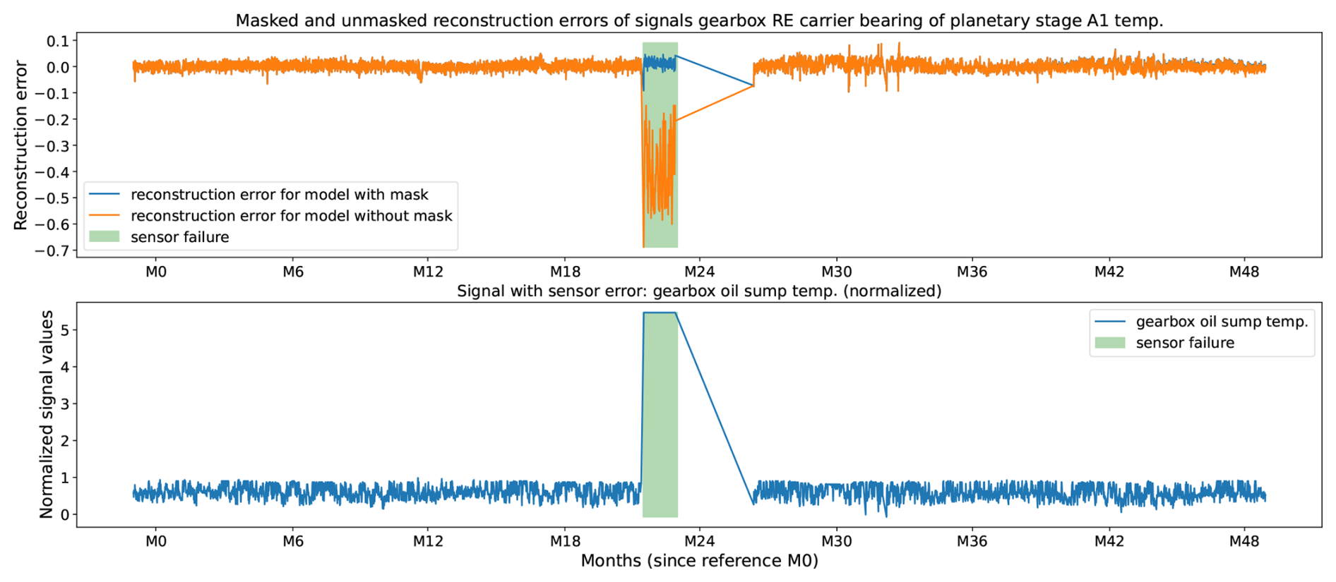
Figure 6 Gearbox oil sump temperature (bottom plot) sensor failure (bottom plot, green box) and its impact (top plot) on the reconstruction error of the gearbox RE carrier bearing of planetary stage A1 temperature (top plot) without (top plot, orange curve) and with (top plot, blue curve) masking of the sensor error. The data originate from turbine 1 of WF1.

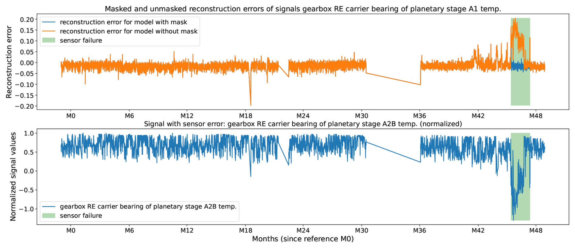
Figure 7 Gearbox RE carrier bearing of planetary stage A2B temperature (bottom plot) sensor failure (bottom plot, green box) and its impact on the reconstruction error of the gearbox RE carrier bearing of planetary stage A1 temperature (top plot) without (top plot, orange curve) and with (top plot, blue curve) masking of the sensor error. The data originate from turbine 21 of WF1.

4 Results

4.1 Distributional similarity of the reconstruction errors under masked sensor error and nominal conditions

The first question examined in this study is whether the reconstruction errors produced by the MAE when at least one sensor has failed remain comparable to those obtained when none of the sensors have failed and the turbine is in a healthy state. Establishing this equivalence is critical: if reconstruction errors differ substantially between these two regimes, it would indicate that the AE has not adequately learned the underlying inter-sensor relationships in the presence of missing or corrupted inputs. In such a case, the reconstruction errors would become unreliable for anomaly detection precisely when sensor faults occur, thereby undermining the purpose of the method.

Figures 6 and 7 provide qualitative insight into the behavior of the algorithm. The bottom plot in each figure shows the normalized signal that is generated by the faulty sensor. The window during which the sensor has failed is highlighted with a green box. The top plot shows the reconstruction errors for a signal different from the one suffering from the sensor failure. The model generates the orange reconstruction error when the data generated by the faulty signal are not masked and the blue reconstruction error when they are masked.

In Fig. 6, the failure occurs in the gearbox oil sump temperature sensor (bottom panel). When the failure is not masked, the corrupted measurement propagates through the learned correlations and induces distortions in the reconstruction errors of other signals, for example, the temperature measured at the gearbox rotor end (RE) carrier bearing of planetary stage A1 (orange line in top plot). These distortions render the anomaly detections for these signals unreliable. Specifically, the failed sensor exhibits a sudden upward bias, which in turn produces an inverted (downward) bias in the reconstructed estimates of correlated signals (orange line in top plot). Because the AE models the normal relationships among these variables, an anomalously high value in one variable prompts overestimation of the corresponding “normal” values of others, leading to negatively biased reconstruction errors. When the gearbox oil sump temperature signal is masked when suffering from the sensor error (green box) the reconstruction error is not influenced by the reconstruction bias, and the error remains in line with the errors outside the green box (blue line in top plot). This indicates that the MAE and the masking of the faulty signal work well.

An analogous but reversed pattern is observed in Fig. 7. Here, the affected sensor, the gearbox RE carrier bearing of planetary stage A2B temperature, shows a pronounced downward bias during the sensor failure window (green box), resulting in upward-biased reconstruction errors in several correlated signals, exemplified in the figure by the reconstruction error for the gearbox RE carrier bearing temperature (orange line in top plot). When the faulty sensor is masked, this upward bias is eliminated, and the reconstruction errors align with the surrounding baseline values (blue line in top plot).

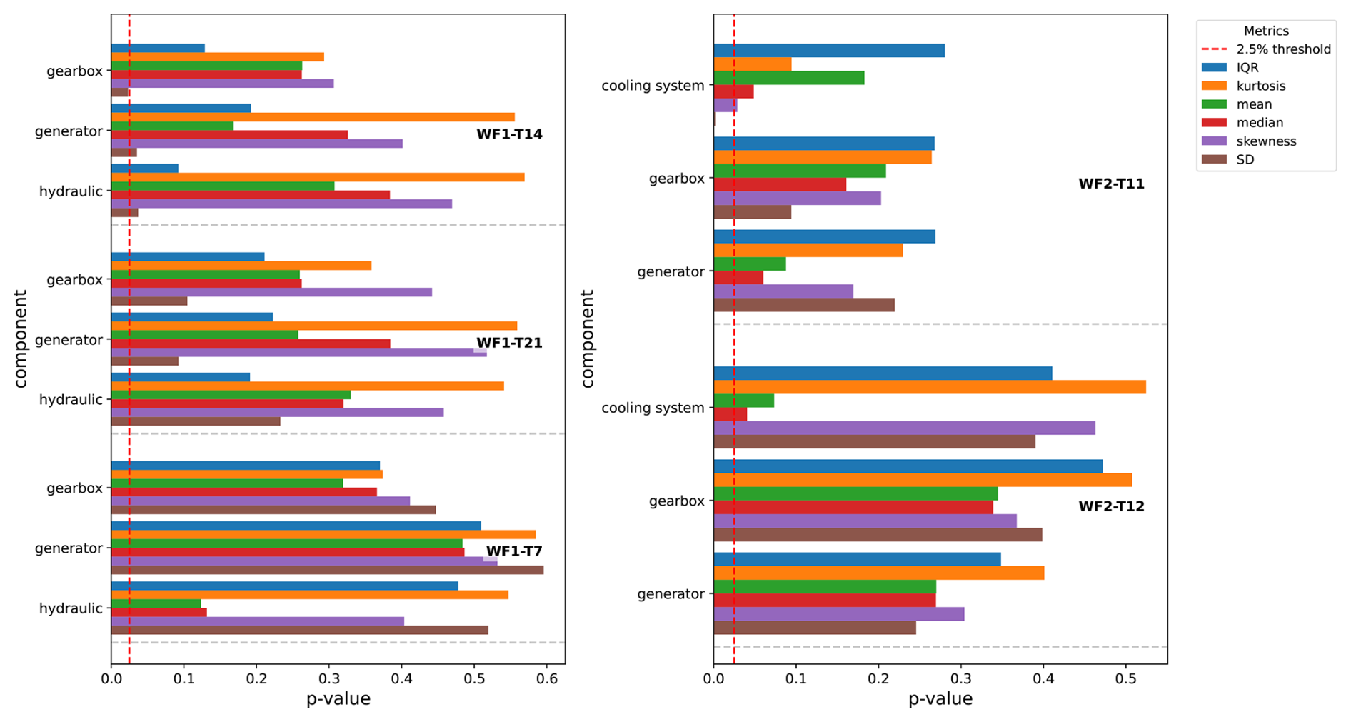
Figure 8 Figure shows for several turbine components, i.e., generator, gearbox, and hydraulics for wind farm 1 (left subfigure) and cooling system, gearbox, and generator for wind farm 2 (right subfigure), the mean of the p values of the KS tests for several distribution-describing metrics, i.e., interquartile range (IQR), kurtosis, mean, median, skewness, and standard deviation (SD). The mean is determined as the average of the p values of the KS tests of the temperature signals that are related to the component (see Tables A1 and A2). The red dotted vertical line indicates the 2.5 % threshold (threshold that separates significant from insignificant evidence against the null hypothesis). The longer the bars, the more similar the metrics are for the reconstruction errors of the signals generated in windows with and without sensor errors. The x axis shows the p values for the different metrics and components. The y axis indicates the component. The colors indicate the metric.

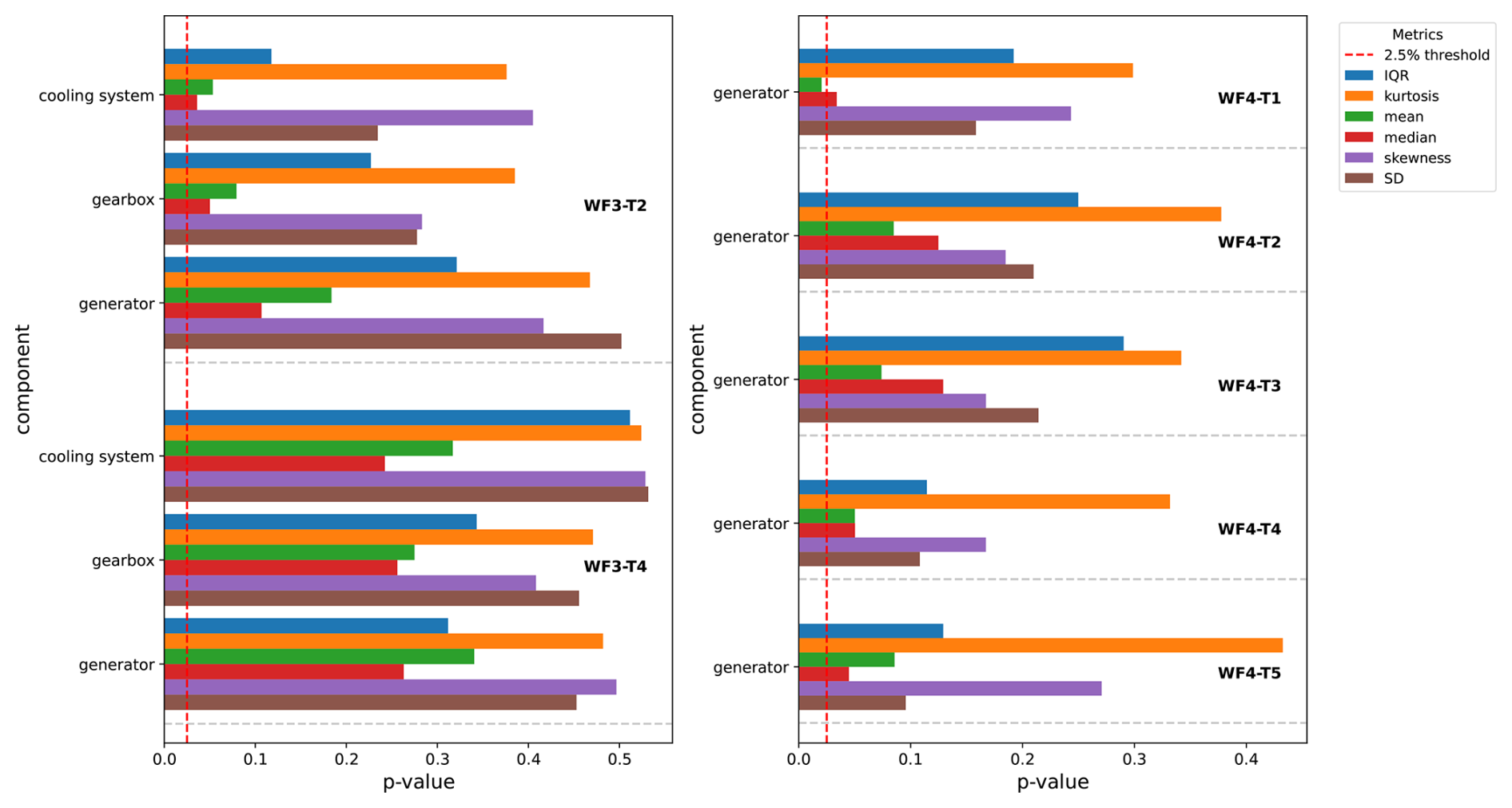
Figure 9 Figure shows for several turbine components, i.e., cooling system, gearbox, and generator for wind farm 3 (left subfigure) and generator for wind farm 4 (right subfigure), the mean of the p values of the KS tests for several distribution-describing metrics, i.e., interquartile range (IQR), kurtosis, mean, median, skewness, and standard deviation (SD). The mean is determined as the average of the p values of the KS tests of the temperature signals that are related to the component (see Tables A3 and A4). The red dotted vertical line indicates the 2.5 % threshold (threshold that separates significant from insignificant evidence against the null hypothesis). The longer the bars, the more similar the metrics are for the reconstruction errors of the signals generated in windows with and without sensor errors. The x axis shows the p values for the different metrics and components. The y axis indicates the component. The colors indicate the metric.

Due to the large number of sensor error validation cases (12 in total), exhaustive visual inspection is impractical. We therefore adopt an automated and formal evaluation based on multiple statistical metrics (see the Methodology section). Figures 8–9 report the average p values (horizontal bars) obtained from KS tests for different subsystems, i.e., the generator, gearbox, cooling system, and hydraulics, and for several statistical descriptors of the reconstruction error distributions, i.e., the mean, median, SD, IQR, skewness, and kurtosis. The purpose of these figures is to assess the similarity of reconstruction error distributions, for signals not suffering from sensor errors, between masked windows containing one or more sensor errors and unmasked windows free of such errors. If the distributions are statistically indistinguishable, the corresponding KS test p values should exceed the 2.5 % significance threshold (indicated by the horizontal reference bars). Larger p values indicate weaker evidence against the null hypothesis of identical distributions. By considering multiple metrics that capture different distributional properties, a more comprehensive assessment of similarity is obtained. For clarity and conciseness, only the average p value per component is shown in the figures.

For validation, 12 sensor error cases were identified. The selection procedure prioritized cases that provide high test quality, requiring that (i) the sensor error period be sufficiently long to extract multiple samples and (ii) enough healthy operational data be available in the surrounding time windows to enable a balanced comparison. Details of this procedure are provided in the Methodology section. The results indicate that, for most components and metrics, the average p values clearly exceed the 2.5 % threshold, implying that the null hypothesis (no difference between reconstruction error distributions with and without sensor errors) cannot be rejected. The consistency of these findings across metrics suggests that there is insufficient statistical evidence to conclude that reconstruction errors differ between data affected by sensor errors and unaffected data. Since the applied metrics characterize complementary aspects of the distributions, these results indicate that the MAE effectively compensates for sensor errors.

In some instances, p values approach or slightly fall below the 2.5 % threshold. There are several possible explanations for this. Firstly, when comparing the p values to the Bonferroni-corrected significance levels, which take into account the multiple hypothesis testing, then none of the p values are smaller than the threshold (0.42 %). However, as stated in the Methodology section, this procedure is very conservative. Secondly, as the data originate from operational wind farms rather than controlled laboratory environments, where unobserved operational events may influence measurements, some fluctuations are expected. A third, farm-specific explanation applies to wind farm 4, which exhibits particularly complex sensor error conditions. In this farm, all gearbox-related signals are missing for an extended period exceeding 2 years, likely due to a persistent communication failure, although the root cause cannot be conclusively determined. As a result, only generator-related results are shown in the right subfigure of Fig. 9. For WF4-T1, the p value for the mean falls below the significance threshold, and the p value for the median lies close to it. Overall, the average p values for wind farm 4 are lower than those observed for the other farms. This reduction reflects the increased difficulty of the scenario, in which approximately half of the input signals are missing. Despite these challenging conditions, the MAE continues to produce reconstruction errors for the generator signals that are broadly representative, albeit with reduced robustness.

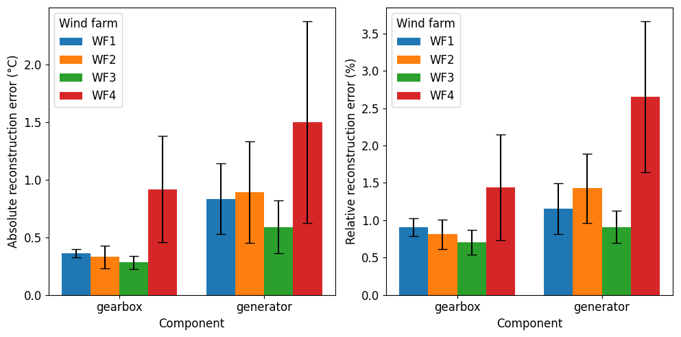
Figure 10 Overview of the absolute reconstruction errors in °C (left plot) and relative reconstruction errors in % (right plot) generated by the model. Each bar color indicates a certain wind farm. The bars are grouped per machine component. The size of the bar indicates the average of the absolute reconstruction errors of the different signals related to the specific component (i.e., gearbox or generator). The whiskers on top of each bar indicate the SD of the average of absolute reconstruction errors of the different signals related to the component.

4.2 Prediction accuracy of model

In this section, we evaluate the modeling performance of the MAE. The assessment is based on the absolute reconstruction errors computed for data classified as healthy. Unhealthy data are identified using the procedure described in the Methodology section. For each signal, both the mean absolute reconstruction error and the mean relative reconstruction error are calculated. The absolute reconstruction error is defined as the absolute difference between the reconstructed and the original signal. The relative reconstruction error is defined as the ratio between the absolute reconstruction error and the corresponding input value. These metrics are subsequently averaged across components, namely the gearbox and the generator. The results are presented in Fig. 10. Overall, the mean absolute reconstruction error is below 1 °C for most cases, with the exception of the generator results for WF4, where it is approximately 1.5 °C. Similarly, the mean relative reconstruction error is generally below 1.5 %, except for the WF4 generator results, where it ranges from approximately 2.5 % to 3.0 %. These findings indicate that the model is able to capture normal operating behavior with good accuracy.

The comparatively lower performance observed for WF4 may have several explanations. First, this wind farm provides the smallest number of available signals for modeling. For instance, only one signal is available per generator phase, whereas two signals are available for the other wind farms. These signals are known to contain complementary information. In addition, many turbines in WF4 are known to experience generator bearing slip. The cause and nature of the bearing slip are currently unknown. The phenomenon manifests as frequent, sudden spikes in bearing temperatures, which are difficult for the model to predict and therefore increase the reconstruction error. Because these events are widespread, they are not fully excluded by the unhealthy data filtering procedure and thus remain present in the dataset considered healthy. This may explain the higher absolute and relative reconstruction errors observed for the WF4 generators.

4.3 Discriminative performance of model in distinguishing healthy and unhealthy data

For failure prediction, it is not sufficient that the model effectively masks sensor faults; it must also reliably distinguish between healthy and degraded operating conditions. Real-world data are not generated under lab conditions. This implies that the data, in this case the temperatures, are influenced by many factors, among which there are factors that are unrelated to the failure cases we use for validation. This might cause temperatures to rise suspiciously and result in anomalies that cannot be correlated with the validation failure cases. However, it would be incorrect to label these as false positives since the temperature increases are real. The validation is further complicated by the fact that these unrelated influential factors are often not all known to us and the industrial partners. This can be due to a lack of information on the occurrence of the event or on the relation between the factor and the temperature signals.

The validation of the methodology is based on generator and gearbox failures. These failures were identified by the industrial partners and are based on actual inspection of the component after the failure. The validation methodology, which is based on the ABSM metric, is tailored in such a way that it measures the actual performance of the algorithm in identifying the validation failure cases as well as possible, with as little influence as possible from the other unknown influential factors. For the analysis of the figures, we focus on the evolution of the anomaly concentration metric just prior to the failure and less on the evolutions far removed in time since those can be caused by the other unknown influential factors.

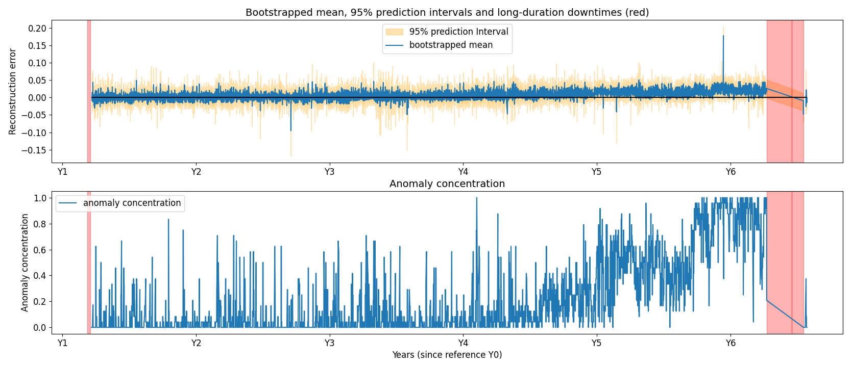
Figure 11 Generator failure for turbine 22 of wind farm 1. The top plot shows the reconstruction error and the 95 % PIs for the generator phase 2 temperature. The bottom plot shows the anomaly concentration score for the same signal.

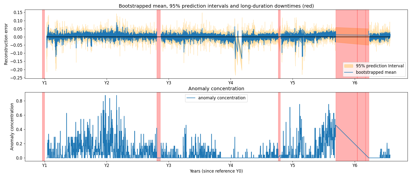
Figure 12 Gearbox failure for turbine 5 of wind farm 1. The top plot shows the reconstruction error and the 95 % PIs for the gearbox RE main bearing temperature. The bottom plot shows the anomaly concentration score for the same signal.

Figures 11 and 12 illustrate examples of correct detections. The top plot in each figure shows (i) the mean of the reconstruction errors generated by the 200 bootstrapped models (blue line) and (ii) the 95 % prediction intervals (PIs) (yellow zone) for a specific signal, namely generator phase 2 temperature in Fig. 11 and gearbox RE main bearing temperature in Fig. 12, respectively. The PIs are generated by calculating the 2.5 % and 97.5 % percentiles of the reconstruction errors generated by the 200 bootstrapped models. These percentiles bound the 95 % PIs. The bottom plot shows the anomaly concentration for the respective signals. An anomaly is identified when the 2.5 % percentile of the reconstruction errors is larger than 0. By using this rule for flagging anomalies, both the trend and the uncertainty are taken into account. The anomaly concentration is the ratio of the number of anomalies versus the number of data points in a 1 d window. This results in a time series with values between 0 and 1.

In Fig. 11, a gradual degradation trend is visible in the anomaly concentration for the generator phase 2 temperature. The trend starts approximately 18 months prior to the failure, which occurred at year 6.25. In Fig. 12, temperatures in the gearbox RE main bearing begin to rise around year 5.5, followed by failure at year 5.75. The detection lead time varies substantially across failures, influenced by many factors that are not always observable. In both of these cases, the model identifies the degradation well in advance. The figure also includes several long-duration downtimes unrelated to the gearbox; these are not detected when using gearbox signals, as the associated failure modes are not gearbox related. In Fig. 12 the anomaly concentration metric also rises around Y2. It is unclear what causes this. There is no evidence that it is caused by seasonal fluctuations since this would also be visible in the following years. An analysis of the event is ongoing.

Table 3 ABSM results for wind farm 1.

Table 4 ABSM results for wind farms 3 and 4.

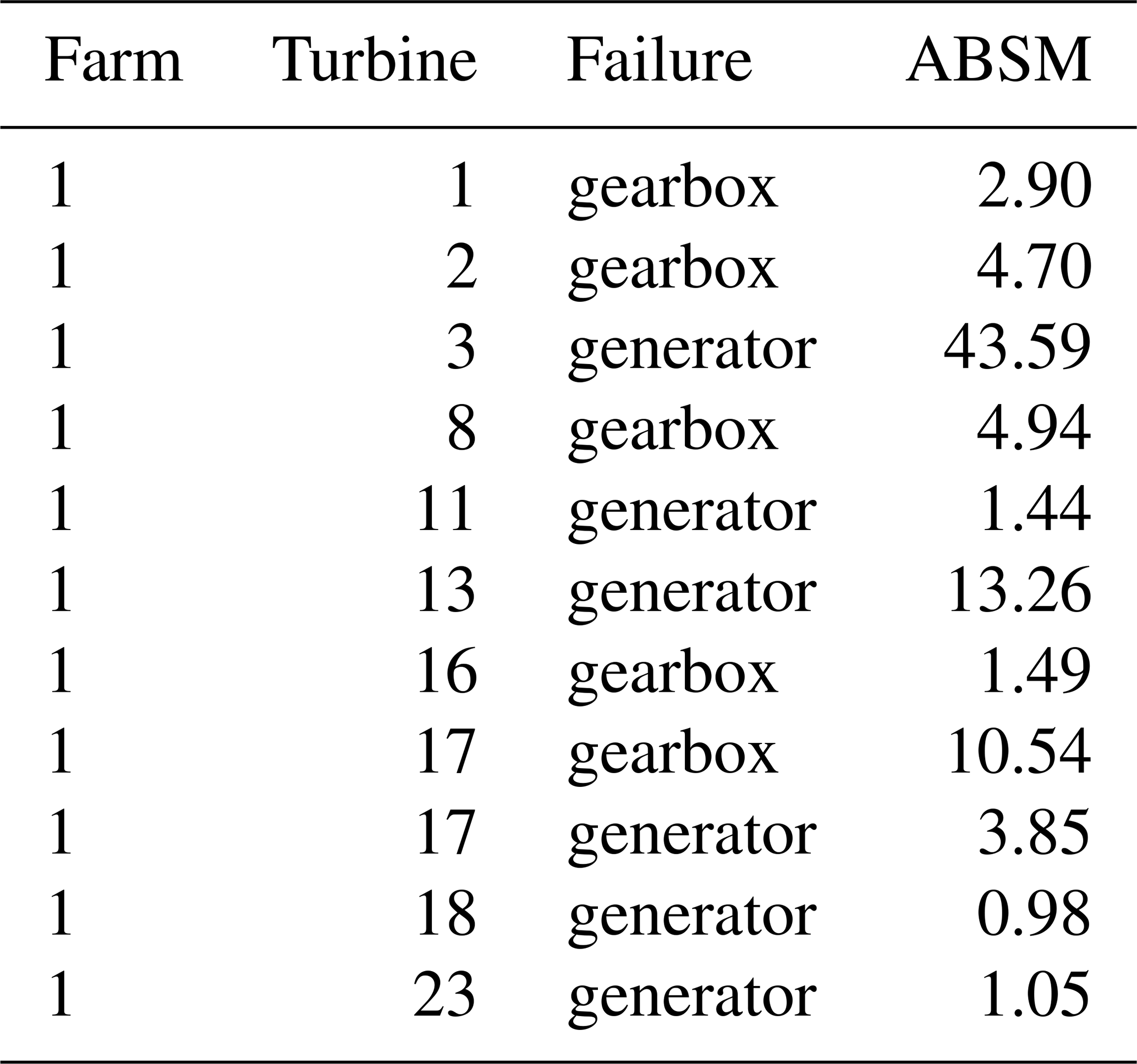
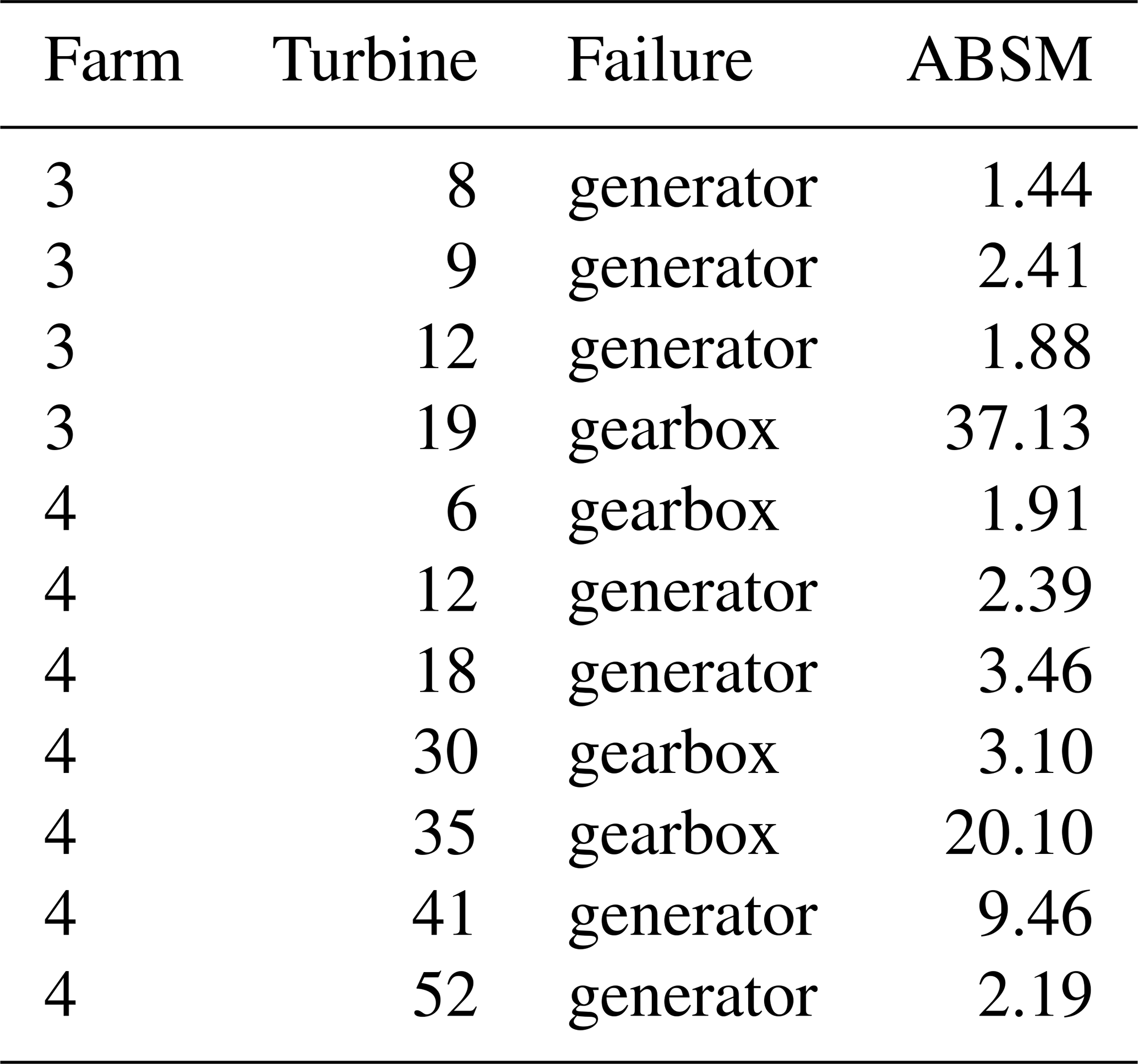
To obtain a general assessment of the value of the model as NBM, we validate it on historical failure data from operational offshore wind farms. For three of the four wind farms described in the Methodology section, industrial partners provided lists containing the turbine ID, timestamp, and failure type. Validation is performed using the ABSM metric (see Methodology section). A strong NBM should yield ABSM values substantially greater than 1 for the component that ultimately fails. In total, 22 drive-train-related failures were evaluated: 9 gearbox failures and 13 generator failures. These failures were provided by the industrial partner. They constructed the list based on post-failure inspections of the components. The results for wind farm 1 and wind farms 2 and 3 are presented in Tables 3 and 4, respectively.

Detection performance is categorized as follows: ABSM >2 indicates a strong detection, 1.25<ABSM≤2 a marginal detection, and ABSM≤1.25 a missed detection. Across all 22 failures, 15 (68.18 %) are strong detections, 5 (22.72 %) are marginal detections, and 2 (9 %) are missed detections, yielding an overall detection rate of 20 out of 22 cases (90.91 %). When split by failure type, the detection rate is 11 of 13 (84.62 %) for generator failures and 9 of 9 (100 %) for gearbox failures.

Overall, the model demonstrates strong discriminative ability. It reliably separates healthy from unhealthy behavior in most cases, with performance somewhat higher for gearbox failures than for generator failures. This difference is expected: several generator failures, particularly in wind farms 1 and 3, stem from electrical issues that are only indirectly reflected in generator-phase temperatures, making early detection more difficult. The two missed detections correspond to generator failures in wind farm 1.

5 Conclusions

This paper presented a sensor-error-robust methodology for failure prediction in wind turbines using SCADA data. Because sensors inevitably degrade or fail during the operational lifetime of a turbine (and because modern condition-monitoring systems rely on large numbers of sensors), the likelihood of encountering faulty measurements is high. The validation data examined in this work contained a substantial number of sensor failures, many of which persisted for extended periods. If left untreated, such failures can significantly distort reconstruction errors and degrade anomaly detection performance. Several examples in this study illustrate how unmasked sensor faults propagate bias into the reconstruction errors of correlated signals, underscoring the necessity of a method that remains reliable in the presence of sensor errors.

The methodology is validated on data and failures from real operational wind farms. The cases used for validation are, on the one hand, temperature sensor failures that have an impact on the performance of the NBM and, on the other hand, drive train failures, i.e., generator and gearbox failures. The focus on wind turbines and drive train failures follows from the availability of failure information and is not due to certain methodological requirements. The methodology can be used on data and failures from other components or machines as long as the data conform to the SCADA data format (time series of signal values) and the model is able to learn the normal or healthy relations between the signals.

The MAE proposed here enables the selective exclusion of corrupted signals during prediction by leveraging a mask matrix that identifies missing or unreliable inputs. This robustness was achieved by training the model on data in which 50 % of the inputs were randomly masked, allowing it to learn inter-signal relationships even under substantial data loss. The results demonstrate that the model successfully maintains consistent reconstruction error distributions when one or more sensors fail. Even in the extreme scenario where all gearbox signals were absent for more than 2 years, the model produced generator signal reconstruction errors of acceptable quality, although with some signs of performance degradation.

The results also demonstrate that the MAE can model the healthy data of the drive train well. In addition, the MAE proved capable of reliably distinguishing healthy from damaged drive trains, even when sensor errors were present. This indicates that the approach is suitable as an NBM. Validation on three operational offshore wind farms, covering both generator and gearbox failures, yielded an overall detection rate of 90.91 %. As expected, detection performance was slightly lower for electrically driven generator failures, which manifest only indirectly in temperature signals.

Several avenues for future work remain. First, the influence of the masking (noise) ratio during training warrants further investigation, as previous studies report effective ratios both lower and higher than the 50 % used here. Exploring this parameter may yield improvements in robustness or detection sensitivity. Second, a more detailed assessment of the stability of the model and uncertainty is desirable. While the current methodology incorporates bootstrapping to characterize stability, further work is needed to translate this stability into calibrated uncertainty estimates and to determine whether additional recalibration methods are required. Finally, evaluating the method on different turbine types and a broader range of failure modes would help establish its generalizability.

Appendix A

Table A1 Component temperature signals for turbines in WF1.

Table A2 Component temperature signals for turbines in WF2.

Table A3 Component temperature signals for turbines in WF3.

Table A4 Component temperature signals for turbines in WF4.