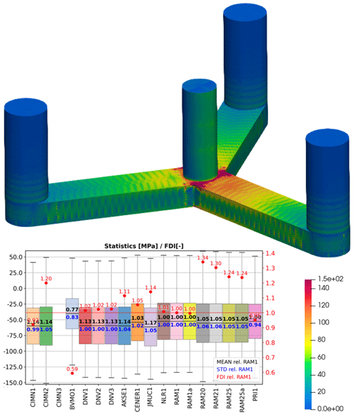
OC7 project Phase II: comparison of global-to-local load transfer approaches in floating structures

Global-to-local load transfer remains a critical – yet largely unstandardized – step in the structural assessment of floating structures. This paper presents the results of package WP2.2 from the OC7 project Phase II, which establishes a cross-industry benchmark for the workflows connecting global performance analysis (based on integrated loads analysis, ILA) and the local structural assessment (based on finite-element analysis, FEA). The study evaluates a spectrum of industry practices, including sequential approaches with the FEA following the ILA, fully integrated time-domain approaches with hydro-structural coupling, and simplified ILA-only approaches. Using the VolturnUS-S reference semi-submersible, the models were first harmonized through mass and inertia, static, and modal verifications. Structural responses were then compared across three primary scenarios: topside-only excitation, irregular waves, and combined wind and wave loading. The results establish a structured comparison framework, highlighting how specific modelling choices and load transfer techniques directly influence confidence in design processes. The findings offer practical guidance to reduce uncertainty in “global-to-local” design workflows.

1 Introduction

The Offshore Code Comparison Collaboration 7 (OC7) project is a large-scale international collaboration conducted under the International Energy Agency (IEA) Wind Technology Collaboration Programme (TCP) Task 56. Its objective is to advance engineering-level, physics-based modelling tools and establish best practices for offshore energy systems (IEA Wind TCP, 2025).

Phase II of the OC7 project is structured into two work packages: WP2.1 (led by the National Laboratory of the Rockies, not in the scope of this paper), covering analysis of member-level loads within a floating substructure (Bergua et al., 2026), and WP2.2 (led by Ramboll, focus of this paper), dedicated to validating the load transfer from global system-level simulations to detailed local structural models (further referred to as “global-to-local” load mapping). This process is critical for assessing structural integrity, especially in floating structures where uncertainties are greater.

While global design and global performance analysis of floating systems have matured significantly in recent years, moving from the global system-level to local stress-level design remains a challenge. Especially beyond the front-end engineering design (FEED) level, detailed structural verifications in ultimate limit state (ULS) and fatigue limit state (FLS) as required by certification societies are challenging to conduct within tight commercial project schedules (Karch et al., 2024). Traditional assessment procedures adopted from fixed-bottom offshore foundations or oil-and-gas sectors are inapplicable, and the existing approaches applied so far have often tried to find a compromise between accuracy and efficiency but have often failed to bridge this gap, leading to either overly conservative designs or severe computational inefficiencies (Karch et al., 2024). Hence, a major effort is currently being undertaken by industry and academia to develop new analysis procedures, with the global-to-local load-mapping process being a key focus.

Yim et al. (2026) demonstrated that failing to maintain strict physical and geometric consistency between global load and local structural models introduces artificial boundary reactions that distort computed structural stresses, which is an important finding relevant for the commonly applied sequential load-mapping approach, where the structural assessment in FEA is separated and follows the global performance analysis (ILA).

Concurrently, as the industry scales up to multi-megawatt capacities, the classical rigid-body assumption for the substructure hull is increasingly challenged. Omitting structural elasticity in global analysis models can compromise structural response predictions. Aguilera et al. (2026) demonstrated using in situ measurements that neglecting floater flexibility introduces significant errors in tower eigenfrequency predictions, whereas incorporating this effect ensures accurate member-level load assessments.

To bypass the steep computational penalties of full shell-element FEA across thousands of time-domain simulations, the industry has turned toward mid-fidelity and reduced-order modelling techniques. Knezevic et al. (2022) established that deploying fully integrated multi-physics methods utilizing reduced basis finite-element analysis (RB-FEA) enables efficient structural integrity assessments without sacrificing geometric complexity. Alternatively, Serván-Camas et al. (2025) proved that leveraging modal matrix reduction methods successfully condenses structural degrees of freedom in coupled aero-hydro-servo-elastic environments, yielding high-fidelity hotspot stress distributions at a fraction of the computational expense. Similarly, Karch et al. (2024) introduced the global influence superposition (GIS) method, a highly efficient unit-load-based approach that maps complex hydrodynamic pressures by applying generalized unit pressure patterns across distinct hull segments, thereby eliminating time-step-by-time-step FEA via linear superposition of scaled unit responses.

Considering fundamental differences between these newly developed analysis procedures, industry stakeholders require verification of their consistency and reliability. Consequently, WP2.2 aims to increase industry confidence in global-to-local analysis workflows by promoting consistency, clarity, and accuracy through shared modelling strategies and verification activities using simulation data from participants to compare the different modelling approaches and workflows in a joint effort. The primary focus of this study is to evaluate the consistency of the different models, while numerical performance, robustness, and efficiency are not considered.

2 Participants and numerical models

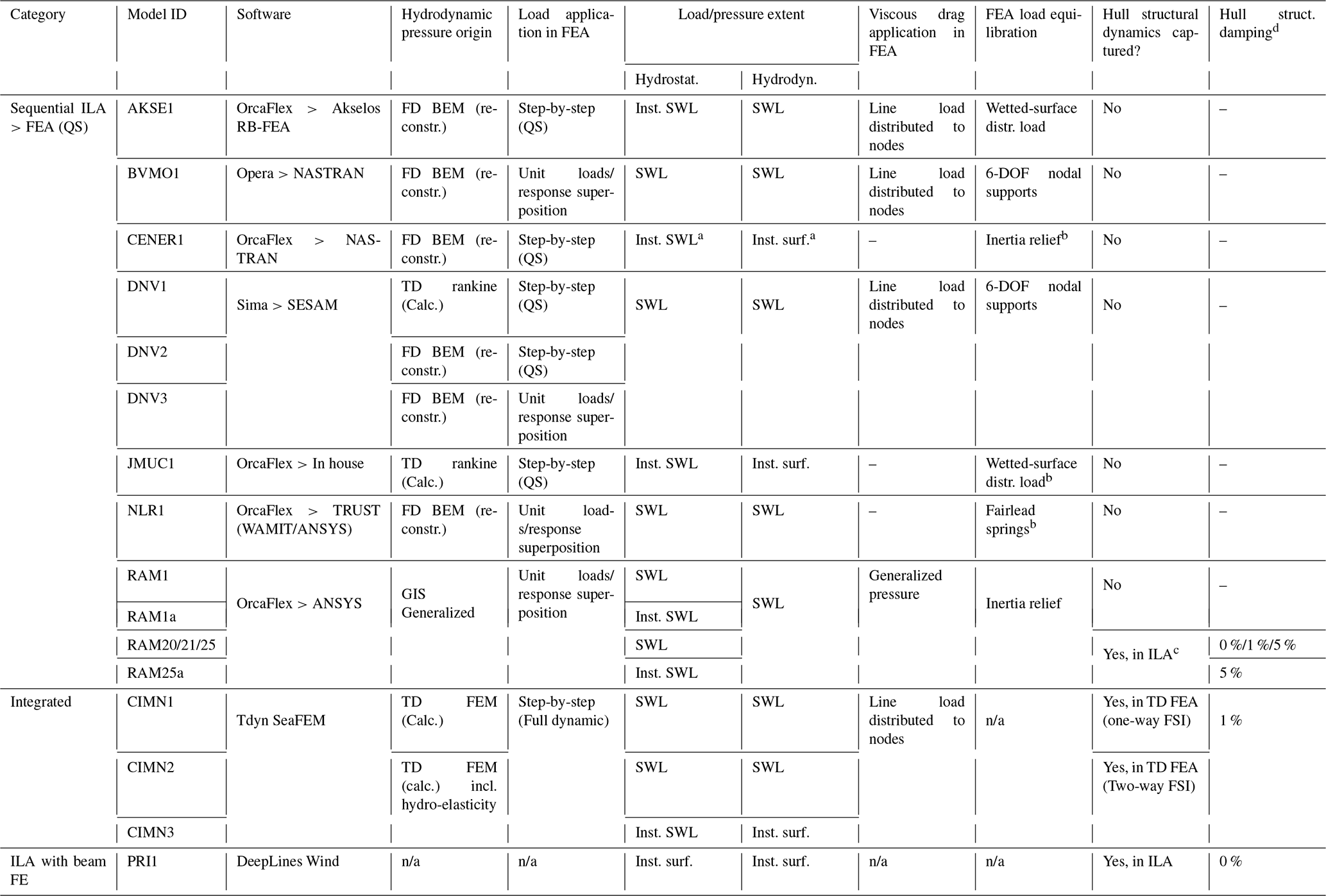
A total of 23 academic and industrial partners participated in WP2.2 from Phase II of the OC7 project. Those actively contributing with results for comparison were, in alphabetical order, Akselos S.A. (AKSE); Bureau Veritas Marine and Offshore (BVMO); Centro Nacional de Energías Renovables (CENER); Centre Internacional de Mètodes Numèrics en Enginyeria together with Universidad Politécnica de Madrid (CIMN); DNV (DNV); the Japan Marine United Corporation together with Nihon Shipyard Co., Ltd. (JMUC); the National Laboratory of the Rockies (NLR); PRINCIPIA (PRI); and Ramboll (RAM). The participants contributed either with one, or – to address the impact of specific model variations and sensitivities – several numerical models; see Table 1 with further modelling details explained in this section below.

Table 1 Model categorization and approaches used.

Abbreviations used:
BEM: boundary element method, DOF: degree of freedom, FD: frequency domain, FE (FEA/FEM): finite-element (analysis/method), FSI: fluid–structure interaction, GIS: global influence superposition, QS: quasi-static, SWL: still-water level, TD: time domain.
^a Pressures set to zero above initial SWL. ^b Expected to be non-negligible as viscous drag is not transferred. ^c Mapped from ILA to QS FEA as inertia load. ^d In % of the critical damping at the first fore–aft flexible eigenfrequency. n/a: not applicable.

The applied numerical models can be categorized based on the general workflow and the level of integration between the global analysis (ILA) and the local structural assessment (FEA) into three main groups:

1. sequential workflow, with separated global analysis (ILA) and structural FEA (i.e. loosely coupled link, indicated by “>” in Table 1);

2. integrated workflow, with global analysis and structural FEA running simultaneously (i.e. strongly coupled link);

3. simplified workflow, without shell-element FEA, with basic structural assessment within the ILA using beam FEM.

The following paragraphs describe each modelling category, highlighting their similarities and specific differences to facilitate the interpretation of the results.

Category 1: sequential workflow

The models assigned to this category are AKSE1, BVMO1, CENER1, DNV1/2/3, JMUC1, NLR1, and RAM1(a)/20/21/25(a) (Bredmose et al., 2024; De Lauzon et al., 2013; Gao et al., 2023; Karch et al., 2024; Knezevic et al., 2022; Touzon et al., 2025; Yim et al., 2026).

This category is used by most participants and appears to represent the current standard industry practice. It involves a sequential workflow where the ILA is conducted first, followed by the FEA.

In most models applied in this project, due to the quasi-static (QS) nature of the FEA, the structural dynamics of the hull are generally not captured in the obtained structural responses. The RAM20/21/25(a) models are an exception, where the global effect of hull flexibility is captured in the ILA and transferred to the QS FEA through inertia loads. In general, methods adopted for DNV1/2, JMUC1, and NLR1 would allow for consideration of structural dynamics via fully dynamic time-domain FEA; however, this feature is not utilized in this project.

By separating the ILA and FEA, the global-to-local link in these models remains relatively loose and relies heavily on the quality of the load transfer (mapping) approach. A critical aspect of this process is the inclusion of all ILA load components; this is essential for maintaining load balance within the FEA. Any imbalances resulting from transfer inaccuracies must be equilibrated through support reactions, inertia relief, or other techniques. However, if a load component is neglected and the resulting imbalance is non-negligible, the equilibration will likely fail to reflect the physical nature of the missing load, ultimately distorting the calculated structural responses. In this regard, it should be noted that models CENER1, JMUC1, and NLR1 do not transfer viscous drag to the FEA; hence, the applied load equilibration technique might become relevant (see Table 1). For other models, the FEA equilibration technique is less relevant as the imbalance is either proved or expected to be negligible.

A major differentiator of the models in Category 1 is the way the hydrodynamic loads from the ILA are converted into pressures (i.e. where the applied pressures originate from). Here, three options exist (see Table 1):

• a.

  Pressures are obtained directly from the time-domain potential flow solution using the rankine source method (DNV1 and JMUC1).

• b.

  Pressures or structural responses are reconstructed via linear superposition of hydrodynamic coefficients or the structural response to these, from the frequency-domain potential flow solution (BEM), scaled by the instantaneous motions and wave data from the ILA (AKSE1, BVMO1, CENER1, DNV2/3 and NLR1).

• c.

  Pressures are reconstructed via linear superposition of generalized pressure distributions (uniform and gradient patterns) on hull segments, scaled by the instantaneous hydrodynamic loads acting on these segments in the ILA, i.e. following the global influence superposition methodology (RAM1(a)/20/21/25(a)).

Furthermore, the models differentiate in the way the pressures, together with other loads, are applied in FEA:

• a.

  The instantaneous loads are directly applied on the FE model, with subsequent FEA, in every time step of the analysis (AKSE1, CENER1, DNV1/2, JMUC1).

• b.

  A set of unit load cases is solved in the FEA once, yielding unit structural responses. The full time history of structural responses is obtained via linear superposition of unit responses, scaled by appropriate scaling factors from the ILA. This method aligns well with the pressure reconstruction strategies (b, c) described above (BVMO1, DNV3, NLR1, RAM1(a)/20/21/25(a)).

Category 2: integrated workflow

The models assigned to this category are are CIMN1, 2, and 3 (García-Espinosa et al., 2023; Berdugo-Parada et al., 2024; Serván-Camas et al., 2025; García-Espinosa et al., 2026).

In the models of this category, a pure time-domain analysis approach is used, combining global response and structural FEA. Hence, the global-to-local link in these models is inherently strong. The structural model includes hull, tower, topside (i.e. rotor-nacelle assembly, or RNA), and mooring lines. The potential flow problem is solved directly in the time domain using the FEM on a fluid volumetric mesh. In the structural solver, a dynamic analysis is performed in the time domain, inherently capturing structural flexibility and structural dynamic effects. Because the fluid and structural solvers are mathematically coupled at every time step, load equilibrium is inherently satisfied without the need for artificial boundary conditions or inertia relief techniques.

The fluid–structure interaction is considered on two levels:

• a.

  The hull is coupled as a rigid body to the hydrodynamic potential flow solution, while elastic deformations have no effect on the fluid pressure (one-way coupling) (CIMN1).

• b.

  The hull is modelled as an elastic body and coupled to the hydrodynamic potential flow solution through generalized structural modes, using an enriched modal reduction approach. This enables a two-way coupling, with elastic deformation affecting the fluid potential field and vice versa (CIMN2/3).

Category 3: simplified workflow, ILA with beam FEM

The model assigned to this category is PRI1 (Defoy et al., 2018; Quideau et al., 2025).

In this category, no external FEA model is used, and no load transfer from ILA to shell-model FEA is done. Consequently, the discussed concepts for pressure calculation/reconstruction, load equilibration, etc., are not applicable. The global-to-local link is inherent but simplified in the way that local structural responses (stresses) are obtained from the global responses/loads. The ILA model differs significantly from the OrcaFlex reference model (see Sect. 6.1); the hull is modelled using skeleton beams, with potential flow multi-bodies attached to them at appropriate locations. The beams are joined using rigid connections, and their stiffnesses are defined based on computer-aided drafting (CAD) geometry to approximate the global structural flexible behaviour. Hence, global structural dynamics are inherently captured within the ILA. The structural responses (stresses) are derived from sectional beam loads (axial and bending) in a simplified way based on classical beam theory. With that, only longitudinal stress components can be retrieved, and the accuracy is expected to be limited around beam joints; i.e. no stresses are available inside the joints.

Disregarding the above toolchain categorization, the different models are further distinguished in Table 1 by the vertical extent of fluid pressure application. Most models (BVMO1, DNV1/2/3, NLR1, RAM1/20/21/25, and CIMN1/2) follow a linearized approach, applying both hydrostatic and hydrodynamic pressure components up to the initial, undisplaced still-water level (SWL). For models based on unit loads/responses, such linearization is usually a common limitation.

In contrast, other models (especially those applying pressures step by step) can capture specific non-linear surface effects:

• Hydrostatic non-linearity. AKSE1 applies hydrostatic pressures to the instantaneous SWL in time domain, considering roll, pitch, and heave motions and accounting for a physically more correct pressure distribution. The unit-load-based models RAM1a and RAM25a also capture this effect by employing a data-driven reduced-order model, utilizing orthogonal eigenpressure modes as unit loads to reconstruct the hydrostatic pressures to instantaneous SWL in the time domain.

• Hydrostatic and hydrodynamic non-linearity. CENER1, JMUC1, CIMN3, and PRI1 further extend fidelity by applying hydrodynamic pressures up to the instantaneous wave surface. While specific implementations vary (e.g. applying only Froude–Krylov forces to the surface while keeping radiation/diffraction terms linear), these models generally aim to consider a physically more realistic pressure distribution than the linear models.

3 Reference model description

This study was performed using the VolturnUS-S reference semi-submersible platform (Allen et al., 2020) with the IEA 15 MW reference wind turbine (Gaertner et al., 2020) (see Fig. 1).

Figure 1 VolturnUS-S semi-submersible platform.

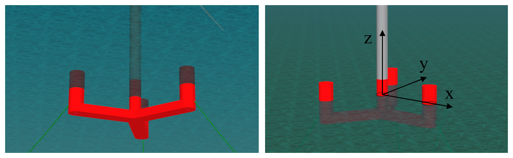
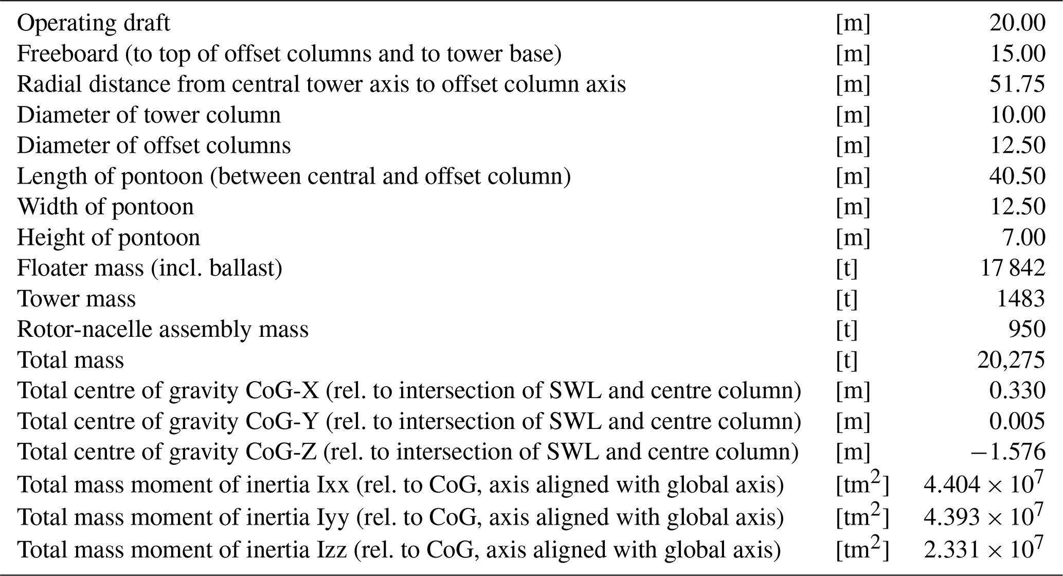
As in WP2.1, the structure was simplified by removing the horizontal braces that connected the top of the columns to the central tower. This was done to (1) simplify the distribution of load paths, making analytical verifications easier, and (2) create a more flexible structure where the effects of structural dynamics are more pronounced and easier to study. The mooring system is a steel chain catenary system consisting of three lines attached to the offset at the top of pontoon level (7.0 m above baseline). The main particulars of the structure are compiled in Table 2.

Table 2 Main particulars of VolturnUS-S reference structure.

4 Load case definition

The load cases considered are compiled in Table 3. The ultimate goal of this study was to assess the impact of the global-to-local (i.e. ILA-to-FEA) load transfer approach on the evaluated structural responses. Load cases (LCs) 6.2, 6.3, 7.2 and 7.3 are of primary interest in this regard, comprising irregular wave excitation with and without RNA load. The other load cases primarily served to align and verify the models and improve understanding of the root causes for deviations between them while generally increasing model complexity within and across load case groups.

Table 3 Load case definitions.

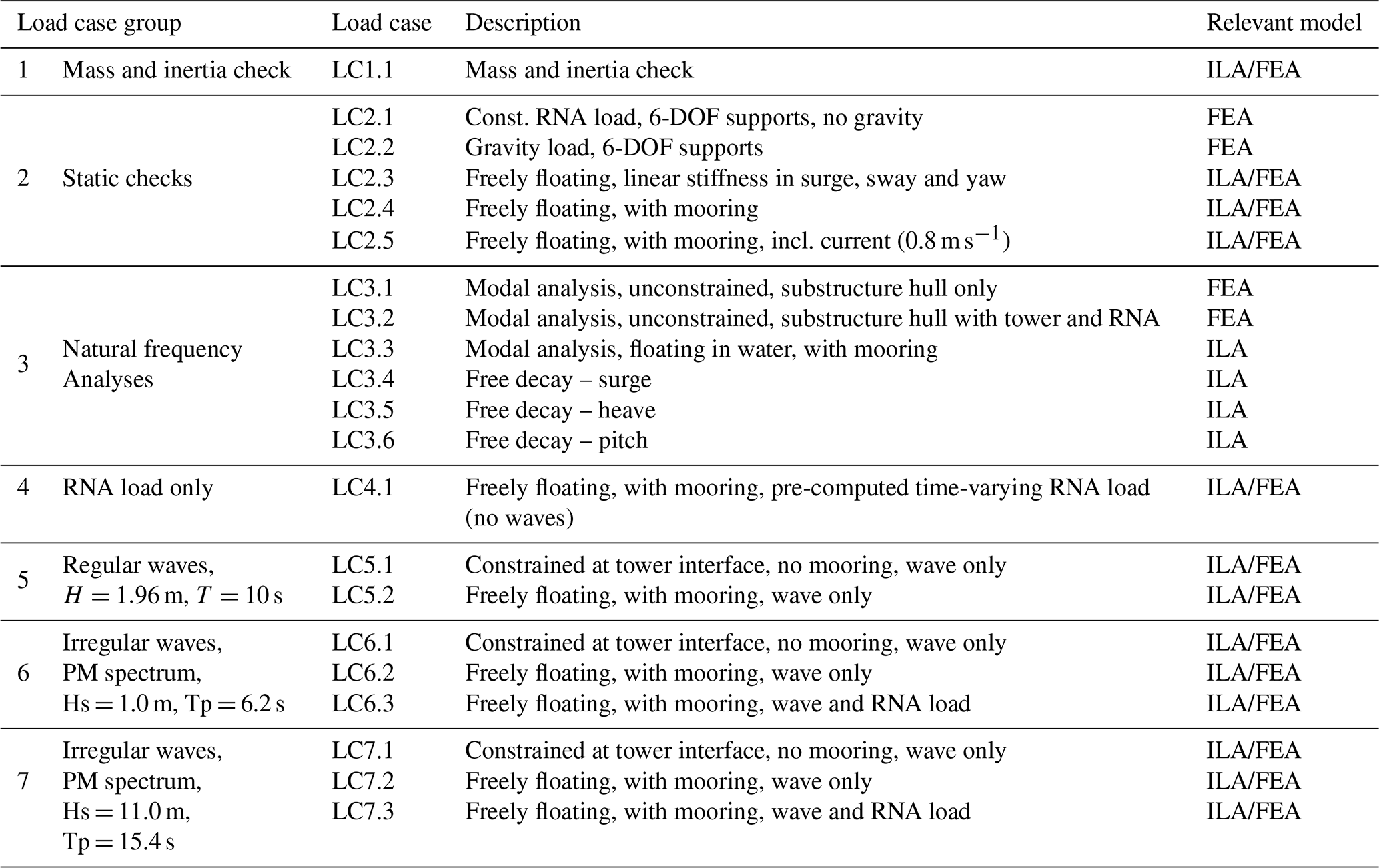
For models with a sequential workflow (Category 1), the load cases were evaluated in FEA, ILA, or in both models with load transfer between them. Simulation durations in LC groups 4 and 5 were 600 and 200 s, respectively. For irregular wave LC groups 6 and 7, the simulation duration was 1200 s, allowing assessment of both the individual wave events and statistics. Modelled water depth was 200 m. All environmental loads (waves, current, RNA load) were applied from the same direction (180°, i.e. towards negative x direction; see Fig. 1). Wind drag was not considered. The RNA load was defined by Ramboll as a pre-computed load time series applied along the rotor shaft axis, based on turbulent wind simulation (mean wind speed of 12 m s⁻¹, Class C turbulence intensity, vertical wind shear exponent of 0.14). This simplified RNA load approach was chosen to eliminate full rotor aerodynamics in the ILA as a potential source of discrepancy between participants' models.

5 Finite-element (FE) models

5.1 Reference FE model

To better align the FE models used in the different toolchains, a reference structural model of the VolturnUS-S semi-submersible was created at the start of the project (see Fig. 2). The structural layout, including plate thicknesses and internal stiffening, was based on minimum scantling requirements and created solely for educational purposes of this project and to maintain consistency across the participants, with no intention of fully complying with any structural rule requirements (i.e. not to be used for a real engineering project).

Figure 2 Reference FE model of the VolturnUS-S semi-submersible.

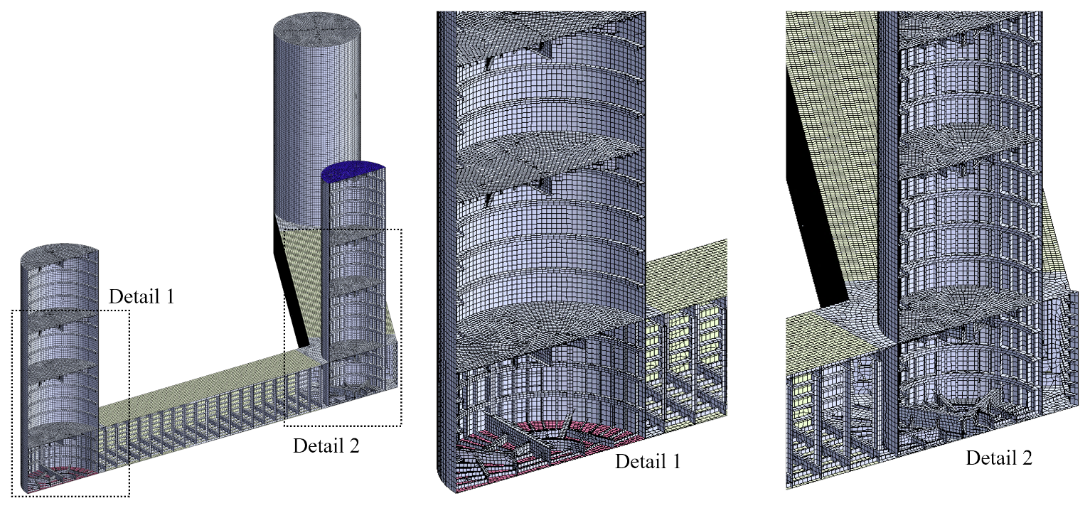
The original VolturnUS-S semi-submersible design has ballast in columns and pontoons to achieve the required operating draft. While modelling of the ballast is straightforward in global response analysis (ILA), its consideration in structural assessments can be challenging. Some tools distribute the ballast mass to nodes of the FE mesh, while others model it as mass points connected to the FE mesh via springs or as pressure distributions. The deviations in the evaluated structural responses introduced by the different modelling techniques can be difficult to isolate and assess and would require another dedicated study. Therefore, the global effect of the ballast was replicated in this study in a simplified way by increasing the material density in different areas of the FE mesh.

The reference FE model consists of 420 672 shell elements (i.e. no 1D beam elements or solid elements) and only includes the hull. The tower and mooring lines are not modelled in FE and are applied as interface loads during ILA-to-FEA load transfer. The model is supported at the base of its three columns, constraining 3 DOFs (x, y, z) at column 1, 2 DOFs (y, z) at column 2, and 1 DOF (z) at column 3. The support conditions primarily affect the static analyses in LC2.1 and LC2.2; in the free-floating cases, the external loads should be in equilibrium, making FE support reactions negligible.

The reference FE model was created by Ramboll in ANSYS and shared with participants in various export formats and as a CAD geometry file to accommodate the different toolchains involved. In all toolchains using a sequential workflow (Category 1), the reference mesh definition could be adopted directly, or similar meshes could be created based on the CAD geometry. The integrated workflow (Category 2) applied in CIMN models required a structural model that included the entire floating structure (hull, tower, RNA, and mooring lines) and therefore had to be extended accordingly. The simplified workflow (Category 3) applied in the PRI1 model does not require a separate structural FEA model.

5.2 FE model alignment verification

The alignment of the applied FEA models was verified based on the following:

• mass and inertia check (LC1.1 in Table 3), which was performed by the participants during FE model creation and is not further detailed in this paper;

• static FE analyses (LC2.1 and 2.2); and

• modal FE analyses (LC3.1 and 3.2).

Since the participant's model variants DNV1/2/3, CIMNE1/2/3, and RAM1(a)/20/21/25(a) share a single underlying FE model, only one variant per participant was evaluated. The PRI1 model does not use a separate FEA model and was therefore not evaluated.

5.2.1 Static FE analyses

For the static FE analyses (LC2.1 and LC2.2), panel-averaged stress components are evaluated. Area-weighted averaging across the elements of one panel was performed to minimize the dependency of results on the mesh density, which differs between participants. Mesh sensitivity analysis was not the focus of the study. The evaluated panels are shown in Fig. 3.

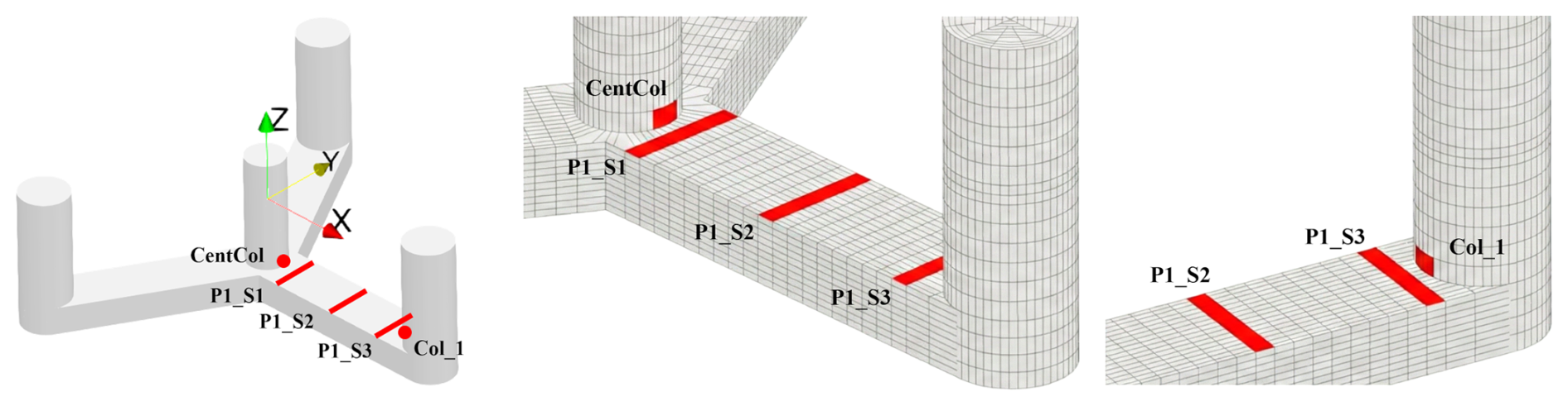
Figure 3 Panel definition for the evaluation of panel-averaged stress components (marked red).

The calculated stress components Sxx (in longitudinal pontoon/column direction) are shown in Fig. 4. Generally, good agreement is observed between the FE models. Any deviations may be due to potential misinterpretations of the definitions of boundary conditions, RNA load application, or stress averaging. The alignment level is deemed acceptable moving forward.

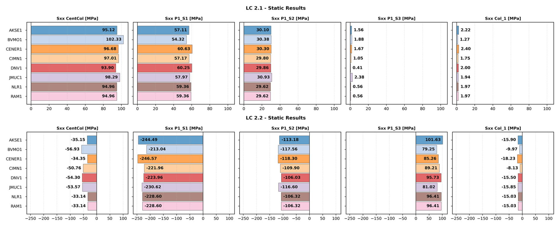
Figure 4 Comparison of panel-averaged stresses (Sxx component) for static load cases LC2.1 (RNA load only) and LC2.2 (gravity only).

5.2.2 Modal FE analyses

The results of modal FE analyses (LC3.1 and 3.2) are shown in Fig. 5. LC3.1 considers a structural model comprising only the substructure hull, whereas LC3.2 additionally includes the tower and a simplified representation of the RNA (modelled as a mass point with associated inertias). The modal analysis is performed in the FEA software without applying boundary conditions (i.e. no supports), assuming a dry structure without hydrodynamic added mass. All FE models show very good agreement in the calculated natural frequencies.

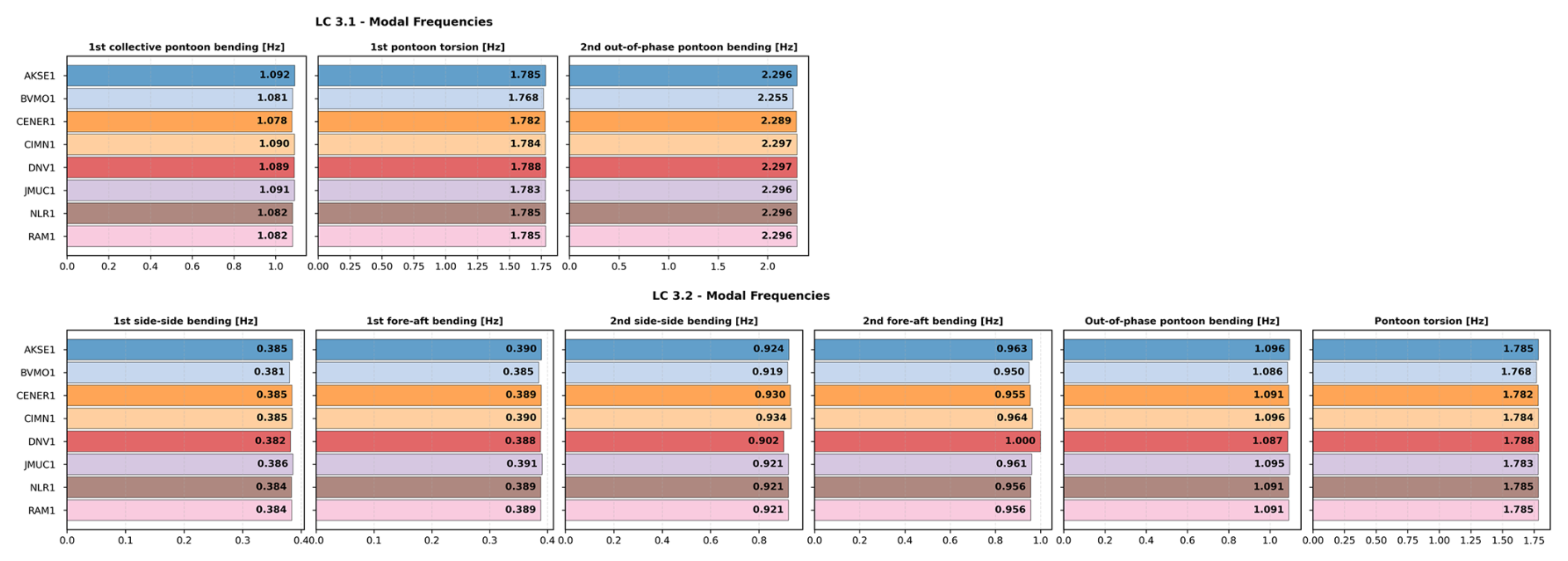
Figure 5 Comparison of eigenfrequencies from FE modal analyses (LC3.1: hull only, LC3.2: hull, tower, and RNA).

6 Global response (ILA) models

6.1 Reference ILA model

To investigate the global-to-local (i.e. ILA-to-FEA) load transfer, it is important that the global basis (ILA) is well aligned between all participants. Therefore, at the start of the project, Ramboll provided the project participants with a reference global response analysis (ILA) model in OrcaFlex software combined with model descriptions and parameter overviews. The modelling details aimed to suffice the common floating wind industry requirements and practices (e.g., hull hydrodynamics based on BEM, consideration of viscous drag, non-linear mooring) while at the same time being relatively simple to better align with capabilities of available load transfer approaches, allowing more institutions to participate (e.g. rigid hull, exclusion of ballast, exclusion of second-order wave loads).

This reference model was used directly by most participants for their analyses. Where specific toolchains required a different ILA software (Opera, Sima, DeepLines Wind, SeaFEM), the respective models were created to adopt (if possible) the OrcaFlex reference model features. Furthermore, some model variations were created by participants on purpose to investigate specific modelling aspects (e.g. hull flexibility, pressure application extent).

For this project that largely focuses on the ILA-to-FEA load transfer, the (hydrodynamic) modelling of the hull in the ILA is of particular interest; mooring lines and tower/RNA modelling are less relevant, as these components are usually not included in the same FEA and considered only via respective interface loads.

In the OrcaFlex reference model, the hull is modelled as a single rigid body. The first-order potential flow loads (radiation/diffraction) are reconstructed from frequency-domain coefficients obtained with BEM: radiation forces are calculated via the Cummins convolution integral, while wave excitation loads are applied via superposition of linear transfer functions. Hydrostatic stiffness is linearized about the initial (undisplaced) floating position. Viscous drag is modelled non-linearly using Morison elements, with drag forces integrated up to the instantaneous water surface using Wheeler stretching. Second-order wave loads are not considered. Mooring lines are modelled with finite elements (OrcaFlex line objects). The tower was modelled as a flexible beam and the RNA as a mass point with inertia and pre-computed load time series (see Sect. 4) applied to it in selected load cases (see Table 3). Wind drag was neglected.

6.2 Global model alignment verification

The alignment of the global response models was verified based on the following:

• static analyses in freely floating conditions (LCs 2.3, 2.4, and 2.5);

• global modal analyses (LC3.3); and

• free decay simulations (LCs 3.4, 3.5, and 3.6; cf. Table 3).

For the comparison, two groups of models should be distinguished where deviations are expected:

1. The first is models aimed to replicate the same features as the OrcaFlex reference model (rigid hull): AKSE1, BVMO1, CENER1, DNV1/2/3, JMUC1, NLR1, RAM1(a). In models RAM1(a), the hull was divided into 14 segments and treated as a multi-body system in the BEM solution. This is necessary for the global influence superposition load transfer approach (Karch et al., 2024). However, since the segments are rigidly connected, the global performance behaviour is the same as that of the single-body reference model.

2. The second is models with features modified on purpose (see also Table 1):

   • RAM20/21/25(a). The same hull segmentation as in RAM1(a) is used but with flexible connections between segments whose stiffness was calibrated to achieve the same modal response (first/second fore–aft/side–side bending) as the FEA model. Model variants differ in the amount of structural damping considered.

   • CIMN1/2/3 and PRI1. The integrated CIMN models and the simplified (ILA with beam FE) PRI1 model inherently capture hull flexibility and structural dynamic effects as well as hydrostatic/hydrodynamic non-linearities (only CIMN3 and PRI1).

Other sources of expected discrepancies are the following:

• Model BVMO1 only considered one drag coefficient (Cd) for the normal direction, whereas the OrcaFlex reference model considers individual coefficients for the horizontal and vertical directions for pontoons.

• Rigid-body motions are reported differently across various flexible-hull models. In models RAM20/21/25(a) and PRI1, this relates to a point fixed on the central column (column axis, at SWL). In models CIMN1/2/3, however, rigid-body motions are extracted directly from the total displacement field using standard FEM procedures, mathematically separating the overall rigid-body movement from the elastic deformation of the hull.

6.2.1 Static analyses in freely floating conditions

Figure 6 shows the rigid-body motions in static freely floating cases LC2.4 (without current) and LC2.5 (with current). While no results for the DNV model were available, other rigid-hull models are generally well aligned. Here, BVMO1 shows some deviations in both cases. Flexible-hull models RAM20 (also representing RAM21/25(a)), CIMN1 (also representing CIMN2/3), and PRI1 show some differences, likely related to the way rigid-body motions are extracted; see explanations above.

Figure 6 Comparison of rigid-body motions in static freely floating cases LC2.4 (without current) and LC2.5 (with current).

In Fig. 7 panel-averaged stresses for LC2.4 are shown (LC2.5 is very similar). The results are generally consistent, showing similar deviations to those observed in LC2.2 (see Fig. 4). The deviations observed in the BVMO1 model for motions are also reflected in the stresses. The beam-based model PRI1 shows deviations in stresses, especially in the pontoon (P1_S1/2/3, see Fig. 3), which are likely inherent in the structural model simplifications.

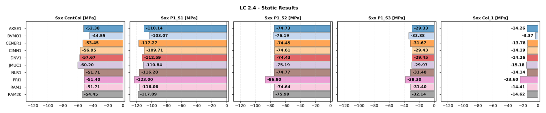
Figure 7 Comparison of panel-averaged stresses (Sxx component) for the static freely floating case LC2.4.

6.2.2 Global modal analyses

The results of global modal analysis (LC3.3) are shown in Fig. 8. All rigid-hull models are very well aligned. The flexible-hull models of CIMN1 (also representing CIMN2/3) and RAM20 (also representing RAM21/25(a)) are well aligned, while the PRI1 model deviates slightly, which is probably caused by simplifications of the beam-based structural model and/or differences in hydrodynamic added mass formulation.

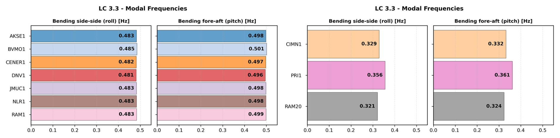
Figure 8 Comparison of first fore–aft/side–side bending eigenfrequencies from global modal analyses (LC3.3) for rigid-hull (left) and flexible-hull (right) models.

6.2.3 Free decay simulations

In Fig. 9 the results of the free decay simulations are shown, i.e. time series (left), statistics (middle), and power spectral densities (PSDs; right). The statistics plots show mean values, standard deviations (coloured boxes), and minimum and maximum values (dashed vertical black lines) for each model. The annotations for the mean (black) and standard deviation (blue) values show the ratio to the RAM1 model, which should be treated as a reference only, for relative comparison. Rigid-body natural frequencies of the floating system (dashed vertical lines) are included in the spectral density plots as reference, i.e. surge 0.007 Hz, pitch 0.036 Hz, and heave 0.049 Hz (Allen et al., 2020).

Figure 9 Free decay results for platform surge (LC3.4), heave (LC3.5), and pitch (LC3.6).

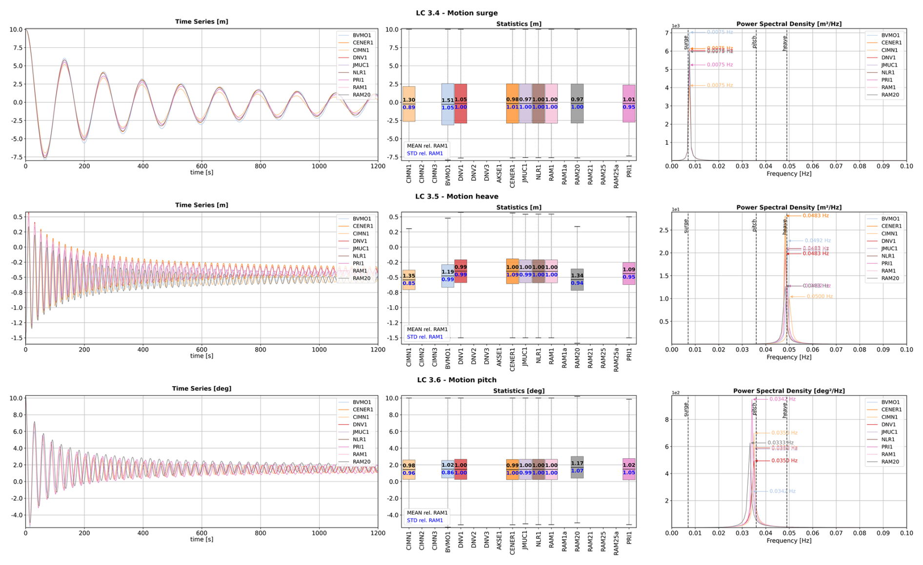
While no results for the AKSE1 model were available, other rigid-hull models are generally well aligned. Here, BVMO1 indicates higher damping in pitch, reflected in a smaller standard deviation value and lower PSD peak, which could be related to the drag coefficient definition (see explanations above). Flexible-hull models RAM20 (also representing RAM21/25(a)), CIMN1 (also representing CIMN2/3), and PRI1 show slight deviations, probably related to the way rigid-body motions are reported (see explanations above) and – in the case of PRI1 – potential implications of non-linear hydrostatics used in this model. While RAM20 and PRI1 indicate higher pitch amplitudes (standard deviation values) for flexible models, CIMN1 shows a distinct response trend.

Overall, while there are some differences between the global response models, the alignment is deemed acceptable moving forward. However, it is expected that the global motion behaviour might deviate significantly in longer irregular wave simulations in groups LC6 and LC7, which are the focus of the following sections.

7 Evaluation of numerical models

After ensuring sufficient alignment between the applied FEA and global analysis (ILA) models, the global-to-local (i.e. ILA-to-FEA) load transfer approaches are evaluated based on stress comparisons in the following load cases:

• LC4.1 (no wave, RNA load only),

• LC6.2/6.3 (irregular waves Hs = 1.0 m, without/with RNA load), and

• LC7.2/7.3 (irregular waves Hs = 11.0 m, without/with RNA load).

Other load cases (LCs 5.1/5.2/6.1/7.1) from Table 3 were used for specific verifications and are not presented in this paper. The results are presented in a format similar to Fig. 9:

• time series plot on the left;

• statistics box plot in the middle, with annotations of mean values (black) and standard deviations (blue) expressed as ratios relative to the rigid-hull RAM1 model for comparison;

• PSD plot on the right, including dashed lines indicating the natural rigid-body frequencies, the global flexible eigenfrequencies (fore–aft/side–side), and the peak frequency of the RNA load.

To make the global performance simulations as consistent and comparable as possible, the RNA load was specified through a pre-computed load time series applied on the rotor; see Fig. 10. The time series plot includes a 15 s zoom-in region (300–315 s). The peak RNA load occurs at a frequency of 0.0017 Hz. With a mean rotor speed of 0.782 rad s⁻¹, the corresponding 3P rotor frequency is 0.373 Hz. This 3P frequency is approximately 15 % higher than the first fore–aft bending eigenfrequency, and it carries only low-energy content (see PSD plot in Fig. 10). Therefore, significant 3P excitation of the tower is not expected.

Figure 10 RNA load time series applied on the rotor in LC4.1, LC6.3, and LC7.3.

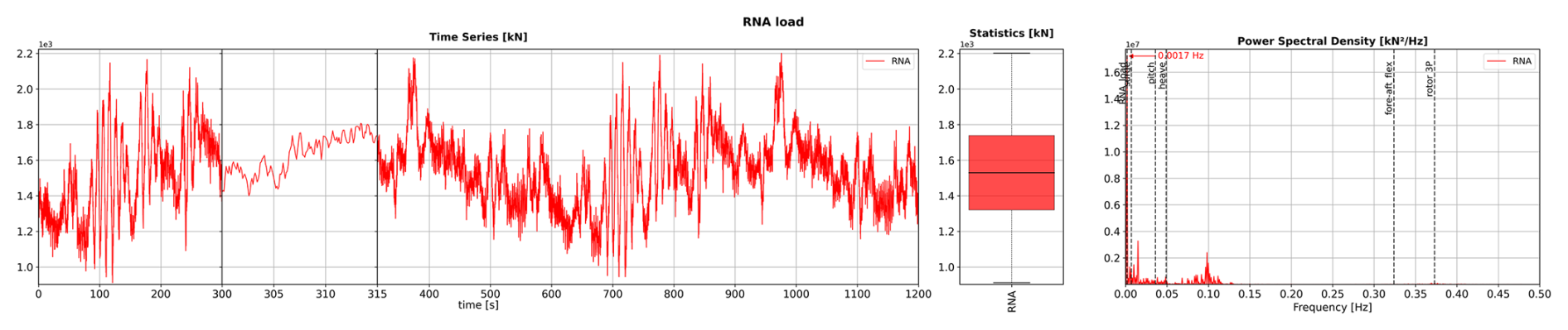
Furthermore, the wave elevation time series (i.e. the amplitudes and phase shift angles of the irregular wave components) were specified as the input data for load cases LC6.2/6.3 and LC7.2/7.3.

Only the most relevant stress results are presented in the following sections. Further results, such as stresses on other panels, sectional loads, and pressures, were evaluated and used to validate and support the derived conclusions.

7.1 Load case LC4.1 (no waves, RNA load only)

Figure 11 shows panel-averaged stress components Sxx (in longitudinal pontoon/column direction) for panels CentCol, P1_S1, P1_S3, and Col_1 (see Fig. 3). As additional information, fatigue damage indicators (FDIs) are included as red dots in the statistics plots. The FDIs are essentially damage ratios relative to the RAM1 model, which is used as the reference for comparison. Damage is calculated based on rainflow counting of stress component time series, considering the S–N curve exponent of m=3. The FDIs are intended solely as qualitative indicators of fatigue damage accumulated in the different models and do not represent a rule-compliant fatigue assessment.

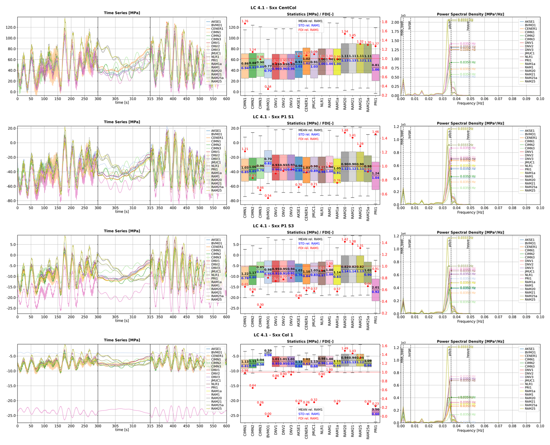
Figure 11 Comparison of panel-averaged stresses (Sxx component) for LC4.1 (no wave, RNA load only).

The time series plots in Fig. 11 reveal discrepancies between the global analysis models discussed in Sect. 6.2. The models based on the OrcaFlex reference model form one cluster (see zoom-in region 300–315 s), with the other rigid-hull models close by, except for BVMO1. All flexible-hull models deviate from this cluster. The statistics plots show that most models are relatively well aligned. Those in the cluster in particular show good consistency in mean and standard deviation values and mostly in FDIs. The statistics of the flexible-hull models CIMN1/2/3 and RAM20/21/25 generally align quite well with these. The flexible-hull PRI1 model aligns well on standard deviation values, while deviating on the mean values.

By comparing RAM20/21/25 with RAM1 (all using linearized hydrostatics) and RAM25a with RAM1a (both using non-linear hydrostatics), it is evident that considering hull flexibility increases the standard deviation values, particularly the FDIs. The amount of structural damping included in the RAM20/21/25 hull models (see Table 1) clearly impacts the FDIs.

A comparison between the CIMN1 and CIMN2 models shows that considering two-way hydrodynamic coupling – where elastic deformations affect hydrodynamic pressures – accounts for the hydrodynamic damping caused by waves radiating by elastic displacements, leading to reduced FDIs and a potentially more realistic representation of energy dissipation mechanisms.

Furthermore, a significant reduction in FDI can be seen in panels P1_S1, P1_S3, and Col_1 of models CIMN3, AKSE1, CENER1, JMUC1, RAM1a, and RAM25a. These models differ from similar ones in how hydrostatic pressures are applied in the FEA. While models such as BVMO1, DNV1/2/3, NLR1, RAM1/20/21/25, and CIMN1/2 apply a linearized distribution, models CIMN3, AKSE1, CENER1, JMUC1, RAM1a, and RAM25a use a non-linear formulation. This leads to different load path distributions within the hull structure (see Fig. 12).

Figure 12 Impact of the linearization of hydrostatic pressures on the load path distribution within the hull structure.

In models with linearized distribution, the hydrostatic restoring moment is generated through negative pressures on the fore column. In models with non-linear distribution, however, it is generated through positive pressures on the aft columns. For LC4.1, the resulting force vector on the fore column is greater for models with a linearized distribution. This increases the sectional loads in the column base and throughout the pontoon sections, consequently increasing the panel-averaged stresses in the respective panels.

The PRI1 model uses a non-linear pressure formulation, and the deviations in stress statistics are likely partially related to this approach. However, the impact of the pressure formulation on the CentCol panel is unexpected; therefore, the remaining deviations are likely due to the simplifications of the beam-based structural model.

The impact of pressure formulation becomes very evident when looking at the sectional bending moments at the base of fore column (Col_1); see Fig. 13 (for CENER1 and BVMO1 no results were available).

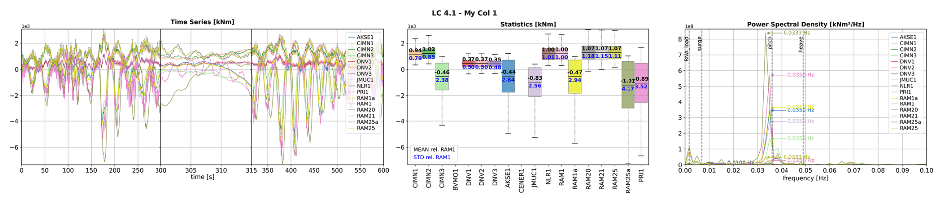
Figure 13 Bending moment at the base of the fore column (Col_1) for LC4.1 (no wave, RNA load only). The effect of non-linear formulation for hydrostatic pressures is evident in models CIMN3, AKSE1, JMUC1, RAM1a, RAM25a, and PRI1.

7.2 Load cases LC6.2/6.3 (irregular waves Hs = 1.0 m, without/with RNA load)

The panel-averaged stresses (Sxx) for the CentCol and P1_S3 panels are evaluated for load cases LC6.2 (without RNA load) and LC6.3 (with RNA load), with irregular waves and Hs = 1.0 m, on a case-by-case basis. This allows the impact of the RNA loads to be assessed directly. Evaluation of the other panels leads to similar conclusions regarding the overall behaviour of the different models and is therefore omitted.

Figure 14 shows the stresses in panel CentCol. Without an RNA load (LC6.2), the tower leans forward, resulting in compressive stresses and small, motion-induced fluctuations from the low-wave-amplitude seaway with Hs = 1.0 m. The stress spectrum is governed by wave excitation and, for flexible models CIMN2 and RAM20/21, exhibits distinct peaks around the first fore–aft bending mode. The RNA load (in LC6.3) leans the tower in the opposite direction and results in tensile stresses with much more pronounced fluctuations (higher standard deviation values). The stress spectrum shows much higher energy content and is dominated by RNA-induced pitch motions.

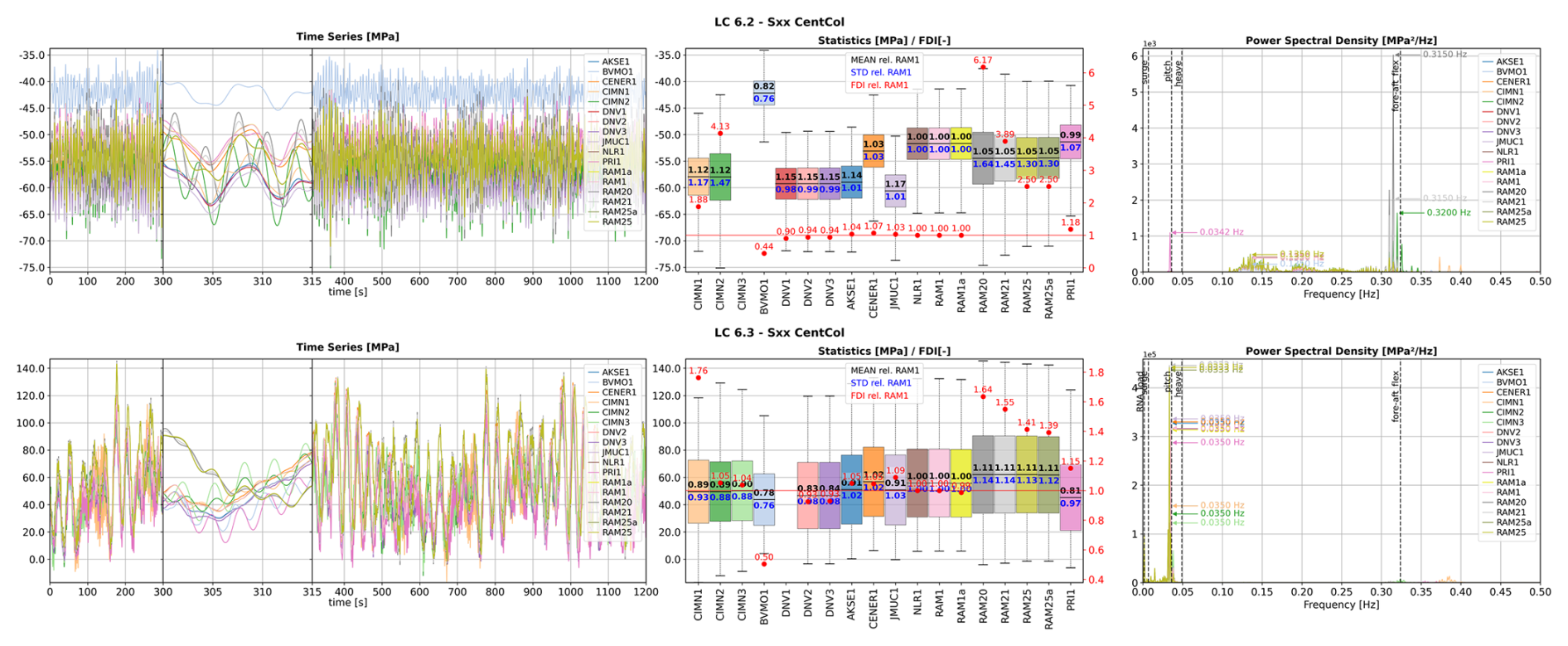
Figure 14 Comparison of panel-averaged stresses (Sxx component) in panel CentCol for LC6.2 (without RNA load) and LC6.3 (with RNA load).

While some differences (especially in mean values) exist, the overall agreement between the models is good. In particular, rigid-body models show good agreement in standard deviation and FDI values. Here, BVMO1 deviates from the others. In LC6.2, the flexible models RAM20/21/25 and CIMN1/2 show significantly higher standard deviation values and FDIs compared to rigid-body models. The RAM20 model without structural hull damping experiences excessive excitations at the first fore–aft bending mode, which reduce with the increased structural damping in RAM21/25 models but are still pronounced. The RNA load in LC6.3 stabilizes the structural response of the flexible models, making the results and conclusions very similar to those from LC4.1 (RNA only).

Figure 15 shows the stresses in panel P1_S3. Similarly to panel CentCol, the stress spectrum is dominated by wave excitation in LC6.2 and by RNA-induced pitch motions with a higher energy content in LC6.3. However, the excessive impact of the structural dynamic effects observed in the flexible models in panel CentCol is not seen in panel P1_S3.

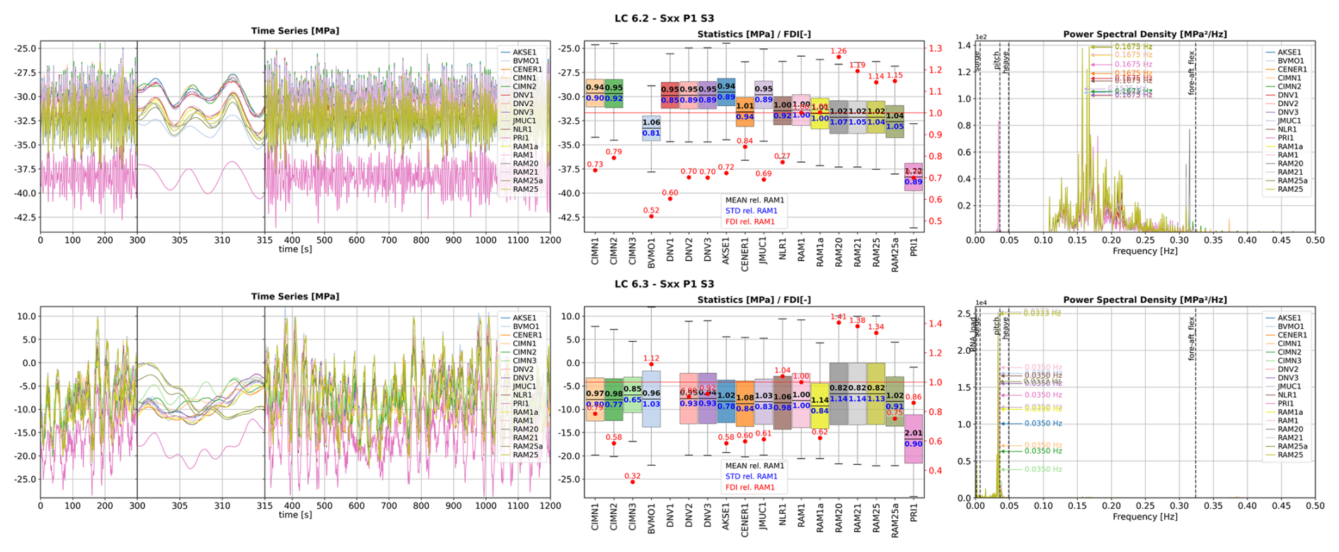
Figure 15 Comparison of panel-averaged stresses (Sxx component) in panel P1_S3 for LC6.2 (without RNA load) and LC6.3 (with RNA load).

Comparing AKSE1, CENER1, JMUC1, and PRI1 results and directly comparing RAM1 vs. RAM1a, RAM25 vs. RAM25a, and CIMN2 vs. CIMN3, it is evident that the hydrostatic modelling strategy (linearized vs. non-linear) has no impact on the CentCol panel (see Fig. 14). In contrast, in panel P1_S3 (close to the fore column), a clear impact of the hydrostatic modelling strategy can be observed in LC6.3 (with RNA load), where the pitch angle is considerable, consistent with the observations from LC4.1 (RNA only).

Including fluid–structure interaction (i.e. two-way coupling; see CIMN2 vs. CIMN1) appears to amplify the FDIs in LC6.2 (wave only), suggesting an increase in wave loads and/or structural oscillations resulting from them. By contrast, in LC6.3, where platform motions are mainly enforced by external RNA excitation, the inclusion of fluid–structure interaction has a damping effect through waves radiated by elastic displacements, thereby reducing the FDIs.

7.3 Load cases LC7.2/7.3 (irregular waves Hs = 11.0 m, without/with RNA load)

Similar to Sect. 7.2, the evaluation of the panel-averaged stresses (Sxx) for load cases LC7.2 (without RNA load) and LC7.3 (with RNA load), with irregular waves with Hs = 11.0 m, is limited to panels CentCol and P1_S3. Evaluation of other panels leads to similar conclusions and is therefore omitted.

Figure 16 shows the stresses in panel CentCol. Without an RNA load (LC7.2), the stress spectrum is completely governed by the high-amplitude wave excitation and resulting floater pitch response, with small peaks around the first fore–aft bending mode appearing in flexible models. The low-frequency RNA load shifts the distribution in the PSD in LC7.3, and the highest peaks occur at the RNA load frequency and the pitch natural frequency. Still, the wave energy content is very pronounced.

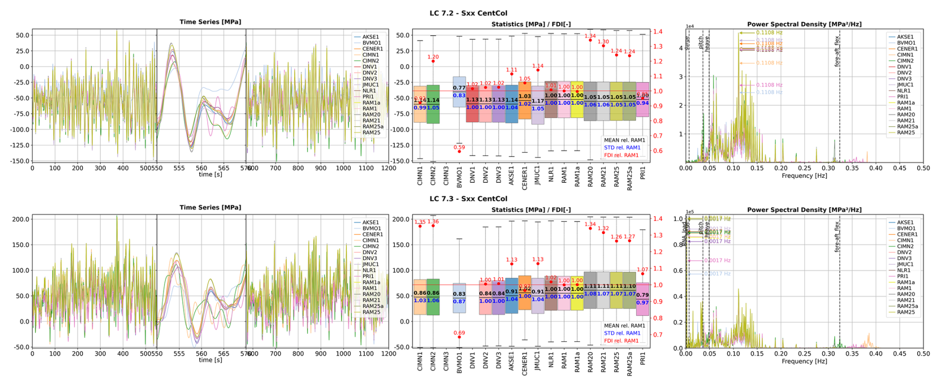
Figure 16 Comparison of panel-averaged stresses (Sxx component) in panel CentCol for LC7.2 (without RNA load) and LC7.3 (with RNA load).

The time series plots in Fig. 16 reveal good overall agreement between most of the models. The time series for all rigid-body models follow a very similar course, except for BVMO1. This is due to the weak alignment of its global analysis model, which is potentially caused by the deviating formulation of the drag coefficients. The flexible models are generally closer to the rigid-body ones and are less scattered than in other LCs. This good agreement is also reflected in the statistics plots, with most mean and standard deviation values being relatively close. This indicates a good alignment between the global analysis models in terms of wave response. Most models compare very well on the applied hydrodynamic loads (radiation, diffraction, and drag), which clearly govern the loads in LCs 7.2 and 7.3.

Rigid-body motions dominate structural responses and structural dynamics, which makes the effect of hull flexibility less visible in time series and standard deviation values. Nevertheless, the FDIs highlight its importance; see the results for CIMN1/2 and RAM20/21/25(a). The FDIs of the flexible PRI1 model do not align with these models, which is probably due to the generally lower accuracy of the beam-based structural model.

The AKSE1 and JMUC1 models have higher FDI values than other rigid-body models. This cannot be attributed to their non-linear treatment of hydrostatic pressures, as this should have no impact on the CentCol panel and is also not observed in other models, such as CENER1, RAM1a, and PRI1, which treat hydrostatic pressures in a similar way.

The results for panel P1_S3 in Fig. 17 lead to similar overall observations. While the time series and the mean and standard deviation value statistics are very well aligned, the FDIs show discrepancies that are, in some cases, significant, even among similar rigid-body models (see BVMO1, DNV2/3, NLR1, and RAM1). These discrepancies cannot be explained by differences in the hydrostatic pressure treatment: RAM1 and RAM25 are similar to RAM1a and RAM25a, respectively, while e.g. AKSE1 significantly deviates from these. They also cannot be attributed to structural dynamics: rigid-body RAM1 behaves similarly to the flexible-body RAM20/21/25, while CIMN1/2 is significantly different.

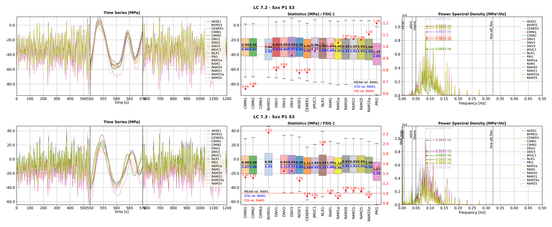
Figure 17 Comparison of panel-averaged stresses (Sxx component) in panel P1_S3 for LC7.2 (without RNA load) and LC7.3 (with RNA load).

The effect of fluid–structure interaction (see CIMN2 vs. CIMN1) in LCs 7.2 and 7.3 is much less pronounced than in LCs 6.2 and 6.3 (Hs = 1.0 m) and is only observed in the increased FDIs of the CentCol panel in LC7.2. This suggests that rigid-body hydrodynamics are the primary contributor to structural loading.

The effect on non-linear hydrodynamics (i.e. the Froude–Krylov pressures applied to the instantaneous wave surface) was expected to be visible in LCs 7.2 and 7.3 (Hs = 11.0 m). However, the relevant models (CENER1, JMUC1, and PRI1) are too inconsistent and do not allow clear trends to be derived in this regard. For CIMN3, no results were available.

One remaining possible explanation for the inconsistencies observed in the calculated FDIs in LCs 7.2 and 7.3 is the difference in FEA load equilibration techniques. This becomes relevant if residual loads arise from the ILA-to-FEA load-mapping process, which is more likely to occur in LC 7.2 and 7.3 environments with high loads and motions.

7.4 Synthesis of observed modelling trends

The comparisons across LCs 4.1, 6.2/6.3, and 7.2/7.3 show that the influence of the modelling technique depends strongly on the governing excitation mechanism. For RNA-load-dominated cases, the treatment of hydrostatic pressures and structural flexibility has a clear effect on stress ranges and fatigue damage indicators (FDIs). For wave-dominated high-sea-state cases, global hydrodynamic loading and rigid-body motions dominate the stress response, while differences in FDI remain sensitive to structural dynamics and local load-mapping details. The main trends are summarized in Table 4.

Table 4 Summary of observed modelling trends in Sect. 7.1–7.3.

8 Conclusions and further work recommendations

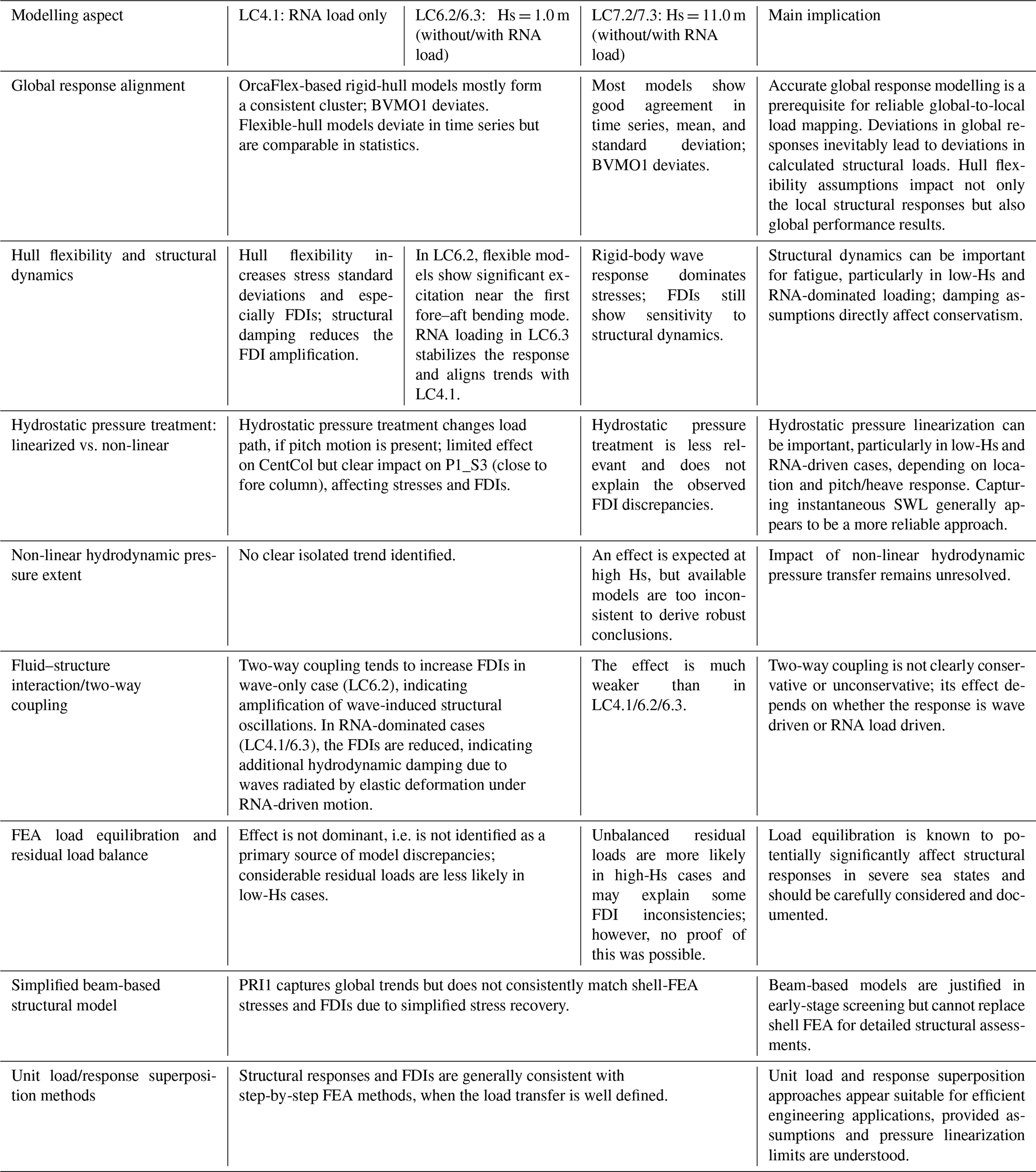
This work investigated a variety of models that approach the global-to-local (i.e. ILA-to-FEA) load transfer and structural assessment in different ways. The models differ in terms of their general workflows, methods for calculating and applying hydrostatic and hydrodynamic pressures, approaches to considering structural dynamic effects, etc. The purpose of this study was not to identify the best model in terms of accuracy, efficiency, or performance. Also, the overall approach and results obtained in this study hardly allow for the selection of the most accurate method, as no real reference exists (e.g. model test based). Nevertheless, the following general conclusions can be drawn from the evaluation of the structural responses calculated with different models:

• The accuracy of the global performance model is the most important factor. It is essential to create an accurate global performance model that adequately captures relevant global load effects to obtain accurate local structural responses.

• Structural dynamic effects contribute significantly to structural responses in some cases, making them important to capture. While the hull structure in this study was intentionally made very soft to better visualize these effects, it is expected that they will not be negligible for most real-world steel floating structures. Their contribution to fatigue in low-Hs sea states appears to be particularly relevant. While different modelling approaches were employed to capture these effects – namely, structural reduced-order models based on generalized modes (CIMN1/2/3) and flexible multi-body ILA models (RAM20/21/25(a) and PRI1) – they all proved effective, though showing some degree of scatter in the results.

• Simplified structural models (such as the beam-based PRI1 model) expectedly yield less accurate results and cannot replace shell-element FE models in resolving the global-to-local load transfer. However, their application may be justified in engineering practice at the early conceptual design stage to increase efficiency and provide high-level identification of structural utilization.

• Linearization of pressures (i.e. application of pressures up to the initial undisplaced SWL) may affect the distribution of load paths within the structure and the calculated structural responses. The significance of this effect is expected to depend heavily on the shape of the hull, the location at which the structural responses are evaluated, and the sea state (i.e. the resulting heave, roll, and pitch motions). In this context, aligning the hydrostatic modelling (linear vs. non-linear) between the ILA and FEA models is advisable to maintain load balance after load transfer.

• Models based on unit loads/response superposition appear to manage the global-to-local load transfer well. While most of these models have some inherent restrictions (e.g. related to pressure linearization), they generally lead to results similar to those of the models solving the FEA step by step. Their application in engineering industry practice appears to be well justified, especially considering their usually substantial efficiency gains.

The study provided valuable insights into the global-to-local transfer of hydrostatic and hydrodynamic loads and highlighted the importance of incorporating structural dynamics. However, as these dynamic effects are not yet fully proven, further verification and validation will be required as methodologies improve.

Most models used in this study were based on linear potential flow solutions, evaluating hydrostatic and hydrodynamic pressures up to the initial undisplaced SWL. While the study successfully isolated the impact of this simplification for hydrostatic pressures, the effects of hydrodynamic non-linearities could not be entirely decoupled. Nevertheless, this modelling aspect is relevant; as observed in WP2.1 (Bergua et al., 2026), incorporating non-linear Froude–Krylov corrections up to the instantaneous water level yielded more accurate results. Therefore, future work focused on transferring non-linear hydrodynamic effects to the FEA level is recommended, potentially benchmarking against computational fluid dynamics.

Furthermore, for the sake of simplicity, the current models did not account for ballast. Considering ballast in structural assessments is not straightforward and can be done in different ways, such as distributing the ballast mass to nodes of the FE mesh or by applying generalized pressure distributions. Studying the effect of different modelling techniques on the calculated local structural responses and their implications for structural design would be beneficial.