Experimental investigation of the rotor–tower interaction of a modern multi-megawatt wind turbine

The increasing demand for a reduction in energy costs per kilowatt hour is leading to larger wind turbines, resulting in longer rotor blades that are also more slender, lighter, and more flexible. These structures are more dynamically responsive and more sensitive to excitations. When a rotor blade passes the tower, an aerodynamic interaction occurs between the blade and the tower, known as rotor–tower interaction. This interaction induces fluctuating loads on both the blade and the tower. Understanding the fluctuating loads on both blade and tower is essential for the design of larger and therefore more dynamically active wind turbines.

To assess how and to what extent the influence of the rotor–tower interaction impacts the structure of modern multi-megawatt wind turbines, in this study, the rotor–tower interaction was investigated by means of pressure measurements on the tower of a modern 4.26 MW upwind wind turbine. For the measurements, a pressure belt, equipped with 36 differential pressure sensors, was mounted on the tower at mid-rotor height. The measurements were conducted over 2 months with the aim of measuring transient surface pressure fluctuations induced by the passing rotor blades. The blade root bending moments recorded by the wind turbine were also examined for selected operating points.

The results show a clear periodic fluctuation of the aerodynamic loading of the tower at the 3P (three times per revolution) blade-passing frequency. Aerodynamic phenomena at the tower, such as velocity excess, stagnation point displacement, and synchronized vortex shedding, which had been predicted in earlier numerical studies, are confirmed by these measurements. The maximum dynamic loads on the tower occur when the turbine reaches its rated power, where the aerodynamic load on the blades is at its highest. The investigation of the blade root bending moment shows that the blade is also influenced by the tower. A fluctuation in the flapwise bending moment of approximately 1 % of the maximum flapwise bending moment is observed when the blade passes the tower. This impact is lower than predicted in several numerical studies, which may be attributed to differences in modeling assumptions and the behavior of a real wind turbine under operating conditions. These findings demonstrate that rotor–tower interaction occurs in modern multi-megawatt wind turbines and can be measured experimentally. Since the observed effect is comparatively small for the investigated turbine type, the results indicate potential for a re-evaluation of blade–tower clearance in modern multi-megawatt wind turbines.

1 Introduction

Wind turbines are subjected to unsteady aerodynamic loads during operation, which are caused by factors such as wind shear, turbulence, and tower interference. In contrast to the unsteady loading caused by inflow turbulence, which spans a wide frequency spectrum, periodic loading induced by wind shear or the tower occurs at multiples of the rotor's rotational frequency (Gómez and Seume, 2009b). Among the periodic sources, tower-induced loading is governed by the aerodynamic interaction between the rotor and the tower's disturbed flow field. The tower alters the surrounding flow field by decelerating the incoming flow on the upstream side and accelerating it around the sides while generating a wake region with reduced wind speed and vortex shedding on the downstream side (Hau, 2016). As a rotor blade passes through this tower-affected region, an aerodynamic interaction between blade and tower occurs, referred to as rotor–tower interaction. This effect arises periodically with each blade passing and induces periodic load fluctuations on the tower at the blade-passing frequency (3P (three times per revolution) for three-bladed rotors).

The mechanisms of rotor–tower interaction vary depending on whether the turbine operates in an upwind or downwind configuration as the rotor blades pass through different regions of the disturbed flow field around the tower. In a downwind configuration, the rotor blades pass through the wake of the tower where a velocity deficit persists. This leads to a temporary change in the effective angle of attack, affecting both the aerodynamic blade loads and the generated rotor torque (Hau, 2016). This periodic blade–wake interaction has been associated with low-frequency acoustic emissions (Madsen, 2010), which contributed to the near-complete disappearance of downwind rotor concepts in large-scale commercial applications (Hau, 2016). In addition, significantly increased fatigue loading has been reported. Zahle et al. (2009) showed that, for a downwind turbine, the blade–wake interaction leads to fluctuations in the normal and tangential blade forces of up to 40 % relative to the free-stream level. A direct comparison of a 1.5 MW wind turbine operating in upwind and downwind configuration, recently made by Bortolotti et al. (2025), shows a similar result. Increases in damage equivalent loads of up to around 25 % were observed. For an upwind turbine, the rotor blades pass through the decelerated incoming flow in front of the tower rather than through the wake. This has a smaller aerodynamic impact on the rotor blade compared to the downwind configuration. Nevertheless, as rotor diameters and hub heights in modern wind turbines continue to increase, maintaining sufficient blade–tower clearance becomes an increasingly critical design constraint (Bortolotti et al., 2025). Therefore, reliable prediction of aerodynamic loading must account for the effects of rotor–tower interaction, even for the predominantly used upwind configuration. Consequently, rotor–tower interaction in upwind wind turbines has been investigated in numerous mostly numerical studies.

The turbines investigated in the literature range from the two-bladed NREL Phase VI turbine with a 10 m rotor diameter to the NREL 15 MW reference turbine with a 240 m rotor diameter, indicating that effects of rotor–tower interaction occur regardless of turbine size. However, the applied simulation approaches differ with respect to modeling assumptions and boundary conditions. The NREL Phase VI turbine represents one of the few wind turbines for which comprehensive and well-documented experimental reference data are available. The objective was to obtain accurate, quantitative aerodynamic and structural measurements of a wind turbine that was geometrically and dynamically representative of full-scale machines at that time. This was achieved by operating it in a wind tunnel under controlled inflow conditions, without turbulence or wind shear (Hand et al., 2001). The wind tunnel measurements obtained for this turbine were used to validate numerical models, which were then used to study rotor–tower interaction under varying inflow conditions. For multi-megawatt turbines, however, the available studies are based almost exclusively on numerical simulations. These simulations have been either validated against scaled model experiments or conducted on purely conceptual reference wind turbines. As these reference turbines do not physically exist, it is not possible to validate the corresponding simulation models experimentally. Accordingly, the reported effects of rotor–tower interaction show a strong dependence on the chosen simulation setup, particularly with respect to the inflow modeling and the consideration of structural elasticity. The most important effects are summarized below.

Several studies show that the rotor–tower interaction leads to periodic fluctuations of the aerodynamic forces acting on the blades as they pass the tower. Simulations by Shkara et al. (2018), Shkara et al. (2020), Kim et al. (2011), and Ghandour et al. (2022) demonstrate that individual blades experience local reductions in aerodynamic forces and moments of 3 %… 9 % when passing through the flow field in front of the tower. These fluctuating aerodynamic loads lead to variations in rotor torque and, consequently, rotor power. Zahle and Sørensen (2008), Shkara et al. (2018), and Shkara et al. (2020) reported rotor torque fluctuations of approximately 2 %… 4 %. Simulations by Horcas et al. (2016) showed rotor power fluctuations of approximately 2 %, while Ghandour et al. (2022) reported fluctuations of up to 7.5 % in a study of a wind turbine scaled to three different rotor diameters (20, 40, and 80 m), and the magnitude of these fluctuations was independent of turbine size. It was also found that the relative magnitude of these fluctuations diminishes with increasing wind speed (Kim et al., 2011; Wang et al., 2012; Hsu et al., 2013).

A direct comparison of the studies by Shkara et al. (2018) and Shkara et al. (2020) shows that the use of elastic rotor blades reduces the influence of rotor–tower interaction on structural loading. Similar observations for flexible rotor blades were reported by Santo et al. (2020). Kim et al. (2011) showed that both increasing yaw misalignment and stronger wind shear lead to a further reduction in the relative influence of the rotor–tower interaction. In both cases, pronounced 1P load fluctuations occur over the entire rotor revolution, meaning the overall loading is increasingly dominated by yawed inflow and wind shear, while the relative contribution of the rotor–tower interaction decreases. Santo et al. (2020) identified an additional influence of the turbine tilt when using flexible rotor blades. The drop in rotor torque induced by rotor–tower interaction decreased from 2.7 % in simulations without tilt to 1.42 % when a tower tilt of 5° was considered. Zahle and Sørensen (2008) performed simulations using a rigid model of a Siemens 3.6 MW wind turbine without tilt. It was found that the tower shadow led to a reduction in thrust and torque of approximately 1 %… 2 % during tower passage.

Fruh et al. (2008), Gómez and Seume (2009a), Gomez and Seume (2009), and Gómez and Seume (2009b) analyzed the aerodynamic interactions between rotor blades and the tower by means of computational fluid dynamics (CFD) simulations. Gómez and Seume (2009b) and Gomez and Seume (2009) explained the interaction between blade and tower as a result of the dynamic change in bound circulation on the airfoil as the blade passes through the altered flow field in front of the tower. According to Kelvin's circulation theorem, a change in bound circulation requires the shedding of vorticity into the flow (analogous to the shed starting vortex by an airfoil accelerated from rest). The effect of the rotor–tower interaction becomes more pronounced with decreasing blade–tower clearance and increasing tower diameter. As a result of the rotor–tower interaction, three phenomena occur on the tower each time the rotor blade passes it (Gómez and Seume, 2009a):

• Stagnation point displacement. The stagnation point on the tower surface is deflected in the direction of blade motion as the blade passes the tower. After the blade has passed, the transient flow dies out and the stagnation point returns to its original position. This periodic displacement of the stagnation point leads to a dynamic change in the pressure field around the tower, which causes pulsating lateral loads on the tower.

• Velocity excess. The aerodynamic interaction of blade and tower causes a local acceleration of the flow on the tower surface, leading to velocities exceeding those predicted by potential flow theory. The strongest flow acceleration occurs at the side of the tower facing in the direction of rotor rotation (i.e., the right side of the tower when the blade passes from left to right). This effect decreases with a larger clearance between the rotor and the tower.

• Wake skewness. The displacement of the stagnation point on the tower surface disturbs the symmetry of the vortex shedding downstream of the tower, temporarily disrupting its periodicity. The result of this is a skewed tower wake.

The simulations also show that vortex shedding from the tower is synchronized with the blade passage. For a three-bladed rotor, a shedding frequency of 1.5P is observed. With increasing rotor–tower clearance this synchronization effect is reduced (Gómez and Seume, 2009b; Gomez and Seume, 2009).

It becomes evident that these studies exhibit a wide variation in modeling assumptions, which leads to corresponding differences in the reported results. The question is therefore how these effects manifest in a real wind turbine under normal operating conditions. To address the lack of full-scale experimental data, this study presents a high-resolution experimental investigation of the rotor–tower interaction on a modern 4.26 MW wind turbine by means of tower pressure measurements using a pressure belt. This study aims to assess whether the effects of rotor–tower interaction are measurable in a modern multi-megawatt wind turbine under real operating conditions by experimentally capturing the aerodynamic phenomena at the tower associated with rotor–tower interaction (e.g., stagnation point displacement and velocity excess). The primary contribution of this study is methodological rather than the provision of a reference database for CFD validation, particularly since the measurement data sets cannot be made publicly available.

2 Experimental setup

To characterize the rotor–tower interaction at a modern multi-megawatt wind turbine, the unsteady pressure fluctuations at the tower are measured. The measurements were conducted at the WiValdi wind energy research farm in Krummendeich, Germany. The wind farm consists of two Enercon E115-EP3-E4 wind turbines, each with a rotor diameter of 115.7 m, a hub height of 92 m, a tilt angle of 7°, and a rated power of 4.26 MW at a rated speed of 13.2 min⁻¹.

Both wind turbines are equipped with extensive instrumentation (recorded at up to 200 Hz), with all measurement data stored in a centralized data management system. Turbine operational parameters, including rotor position, blade root bending moments, and pitch angles, are recorded at a sampling rate of 100 Hz. In the main wind direction, a meteorological mast is located 234 m upstream of the first turbine (OPUS 1), recording the atmospheric conditions at 10 Hz. At the time of the measurements, one cup anemometer at 33 m height and three cup anemometers at 91 m height were in operation. All measurement systems are time-synchronized (Jessen et al., 2025).

To measure the flow around the tower, a pressure belt was designed at the Institute of Turbomachinery and Fluid Dynamics of Leibniz University Hannover and installed on the tower of turbine OPUS 1 in March 2023 (Fig. 1). The belt was installed during turbine assembly while the tower segment was stored horizontally on the ground. After assembly, the belt is located at a height of 59 m above the ground, at mid-rotor level (Fig. 2). The belt is 50 mm thick, has a total length of 13.2 m, and encircles the tower. A total of 72 pressure ports with a diameter of 4 mm are integrated into the belt, of which every second port was equipped with a sensor for this measurement campaign. The 36 differential pressure sensors measure the pressure difference between the outer tower surface and the interior of the tower. The distribution of the sensors around the tower in the earth-fixed coordinate system is shown in Fig. 3. To minimize distortion and response time of the pressure signal through the sensing tubes, the sensors are located less than 10 cm from their corresponding pressure ports in the belt. The differential pressure sensors used (Amsys AMS 4712-0050-D-B) have a pressure range of ±5000 Pa. All sensors share a common reference pressure line routed into the inside of the tower.

The measurement data for this study were collected in the period from 18 September 2024 to 19 November 2024. Throughout the entire measurement campaign, two sensors were identified as outliers. These sensors were excluded from the analysis entirely and are highlighted in red in Fig. 3.

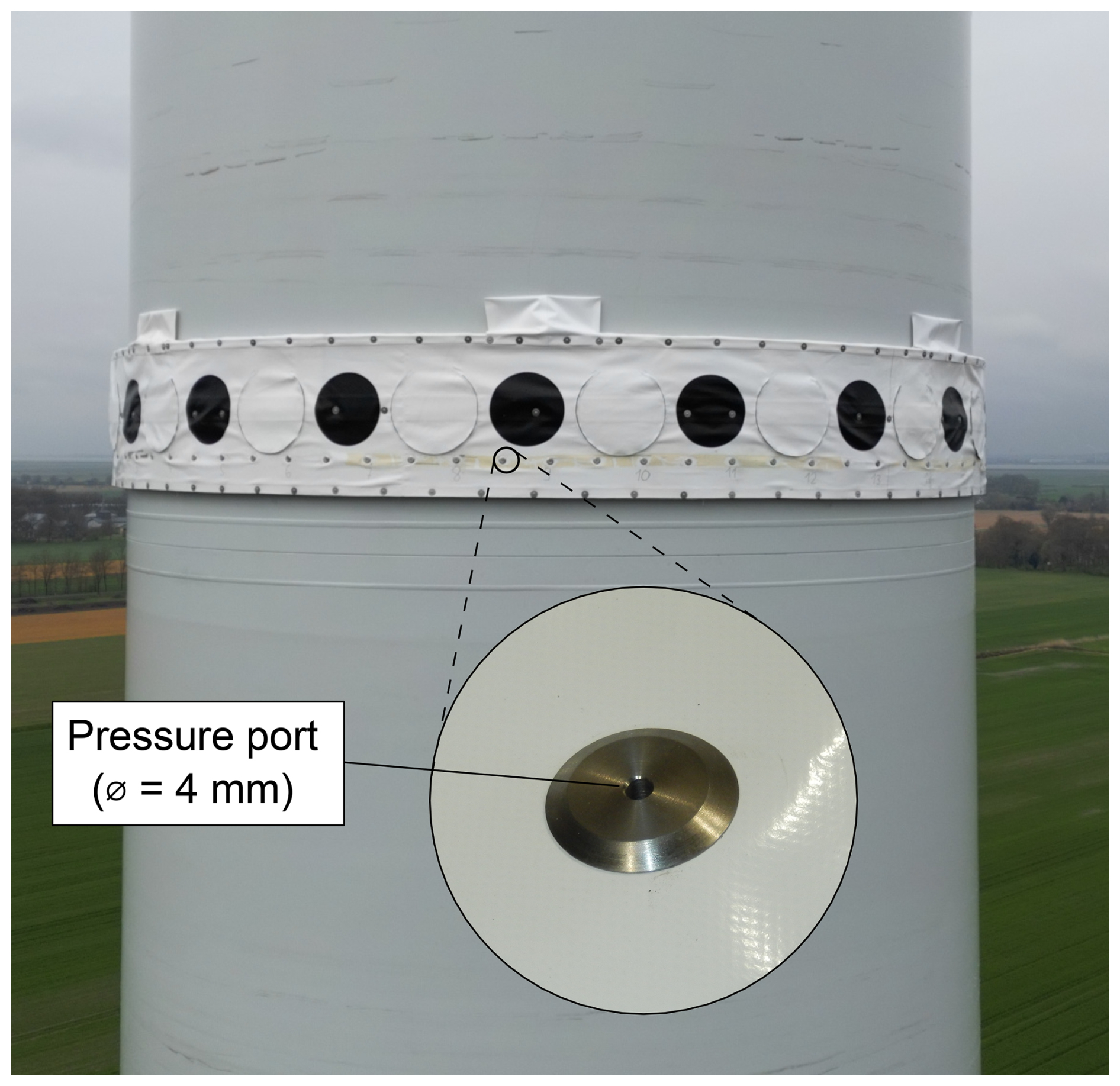
Figure 1 Pressure belt installed on the tower of OPUS 1. The pressure ports have a diameter of 4 mm. A total of 72 pressure ports are integrated into the belt, of which 36 (every second port) were equipped with sensors for this measurement campaign. The black markers are used for digital image correlation (DIC) measurements and were not considered in this study. Photo credit: Kevin Gnebner, DLR.

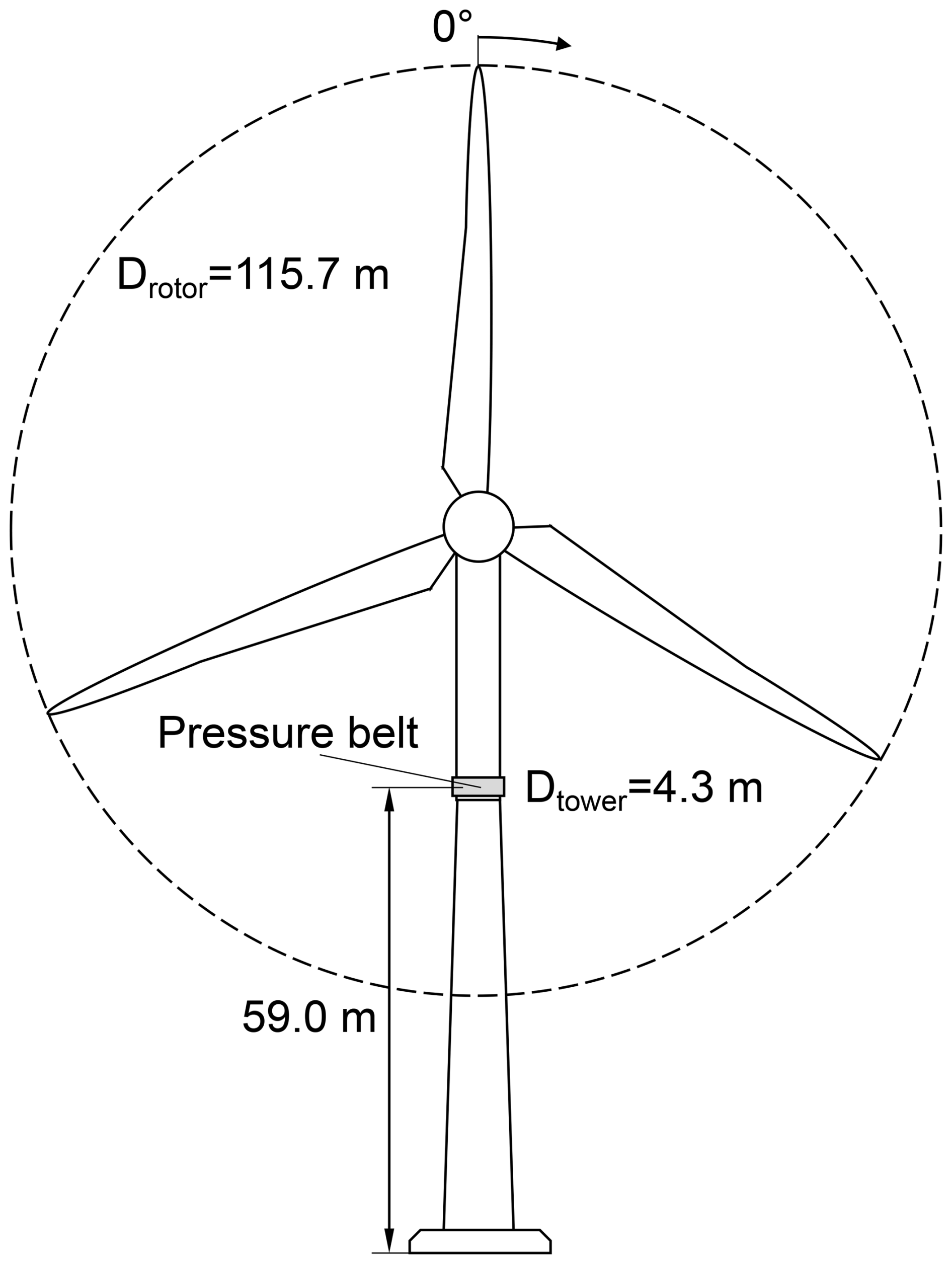
Figure 2 Position of the pressure belt on the tower of the wind turbine and definition of the rotor position. A rotor position of 0° corresponds to the 12 o'clock position. Positive angles are defined in the direction of clockwise rotation (forward-looking aft).

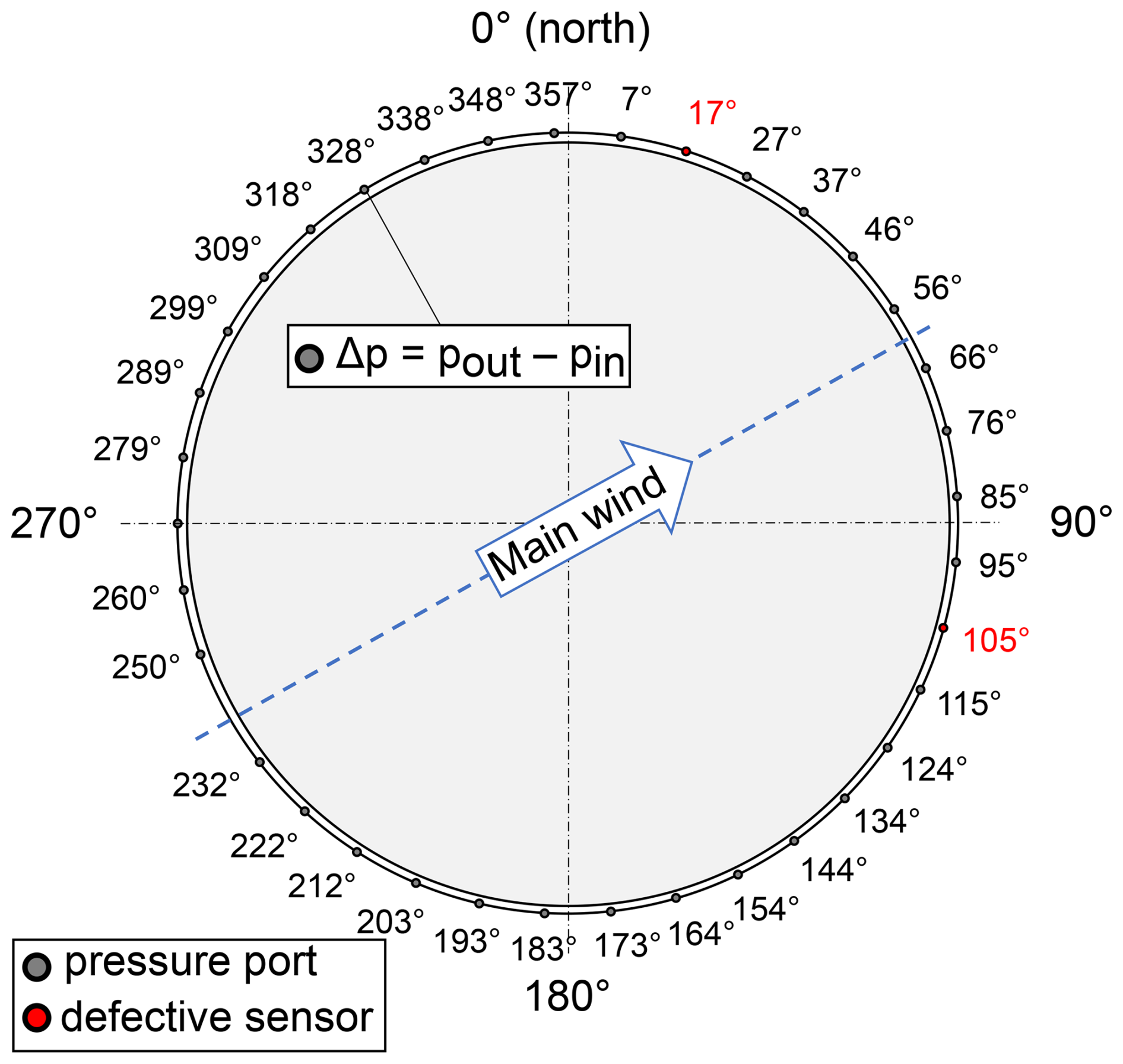
Figure 3 Distribution of pressure ports on the belt in the earth-fixed coordinate system (0° facing north). The differential pressure is measured between the tower surface (p_out) and the inside of the tower (p_in). Two defective sensors (marked in red) were excluded from the analysis.

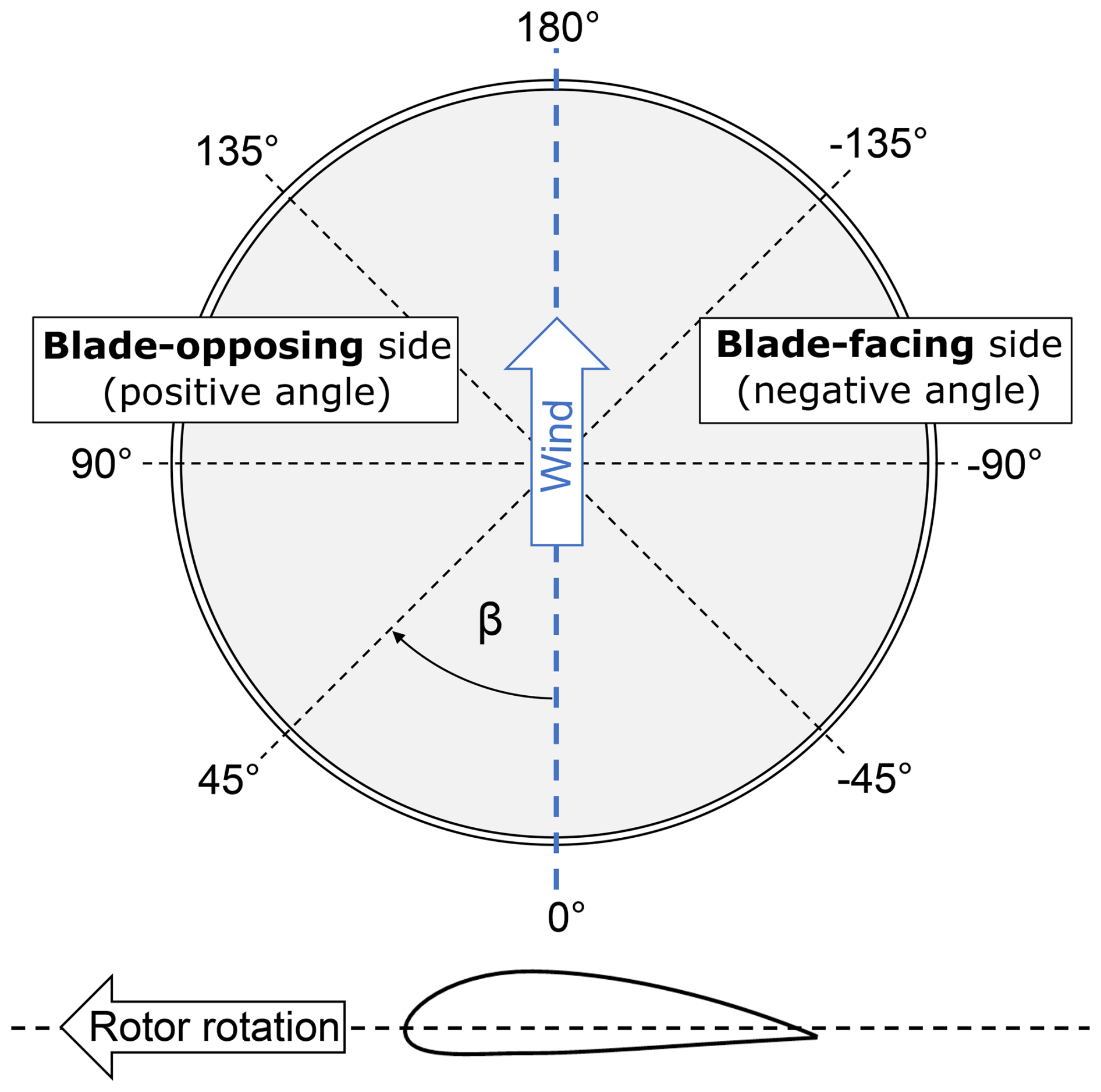
Figure 4 Definition of angle conventions for pressure signals aligned with the wind direction: wind is assumed to come from 0°. The blade passes the tower from right to left. A negative angle β corresponds to the blade-facing side, while a positive angle corresponds to the blade-opposing side.

According to the manufacturer, the sensors have a specified absolute measurement uncertainty of ±50 Pa. Before installation, the sensor calibration was tested over their whole range in 1000 Pa steps, indicating a linear response. At the start of the measurements on the wind turbine, pressure fluctuations below 50 Pa were observed, which were successfully resolved by the sensors. Since the belt had already been installed on the turbine, it was no longer possible to access the sensors directly. Laboratory tests using two identical sensors confirmed that the sensors also show a linear response in the low-pressure range below 50 Pa. However, individual sensors showed different offsets at a differential pressure of 0 Pa. An example of a sensor's response curve is shown in Fig. 5, where the offset is clearly visible. The scatter of the data points in this figure is caused by the pressure gauge used in the laboratory tests, which has a maximum resolution of 10 Pa. A linear fit of the data shows a coefficient of determination of R²=0.9996, indicating a linear sensor behavior. It was therefore concluded that these sensors can resolve the relevant pressure levels by performing an additional zeroing and calibration of the sensors.

To estimate the offset of the sensors already installed on the tower, time intervals with no wind were identified. Since the internal tower reference pressure was not measured but all sensors reference the same internal pressure, one sensor was selected as a reference. The offset of all other sensors was then determined relative to this sensor. For each sensor, at least 400 000 samples were analyzed across 4 different days between May and November 2024. The resulting offsets are shown in Fig. 6. Based on the standard deviation of these measurements, the individual uncertainty of each sensor was re-evaluated. Sensor no. 26 showed the highest standard deviation of 3.72 Pa. From the standard deviation, the 95 % confidence uncertainty was calculated using a t factor of 1.965. A measurement uncertainty of 7.3 Pa with an individual offset was then used for every sensor.

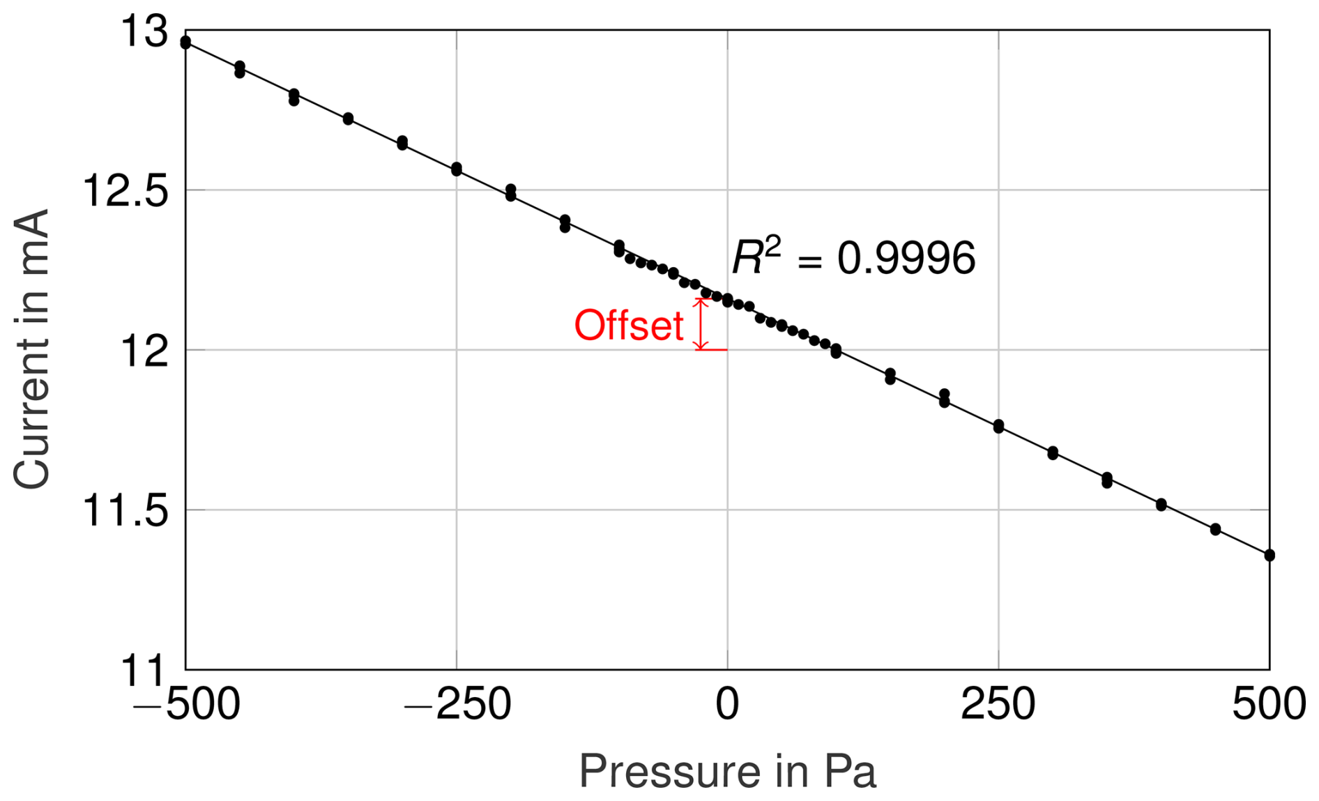
Figure 5 Sensor characteristic curve determined in the laboratory for the range of −500…500 Pa. The offset at a differential pressure of 0 Pa is clearly visible.

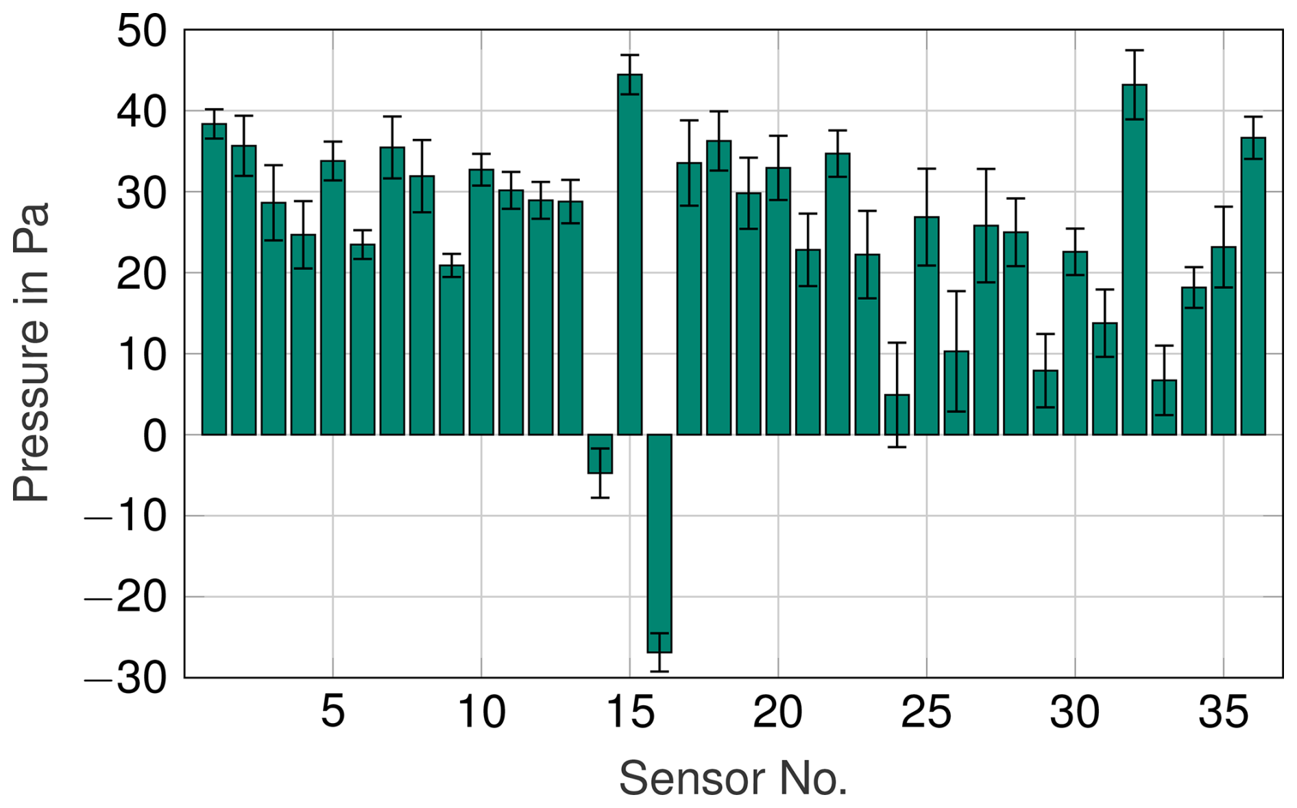
Figure 6 Zero pressure offsets of all 36 pressure sensors. The error bars indicate the measurement uncertainty in the 95 % confidence interval.

3 Data processing and analysis

Two types of analyses were performed: one based on high-resolution data divided into 10 min windows and another based on long-term data averaged in 1 min bins. In both cases, the data were filtered to exclude periods with non-operational turbine states (e.g., idling or throttled power) or periods with missing sensor data (e.g., due to outages and maintenance work).

For the high-resolution analysis, 10 min averages of the filtered data over the entire measurement period were grouped into wind speed bins with a width of 1 m s⁻¹. Within each bin, the 10 min intervals were ranked based on the standard deviation of the wind speed. This allowed the identification of one representative 10 min interval per bin with the most stable wind conditions. The high-resolution data from these selected intervals were then used for further analysis. The extracted 10 min intervals for this study are shown in Table 1.

Table 1 Operating points with high-resolution data. The 10 min mean values ± standard deviation are shown.

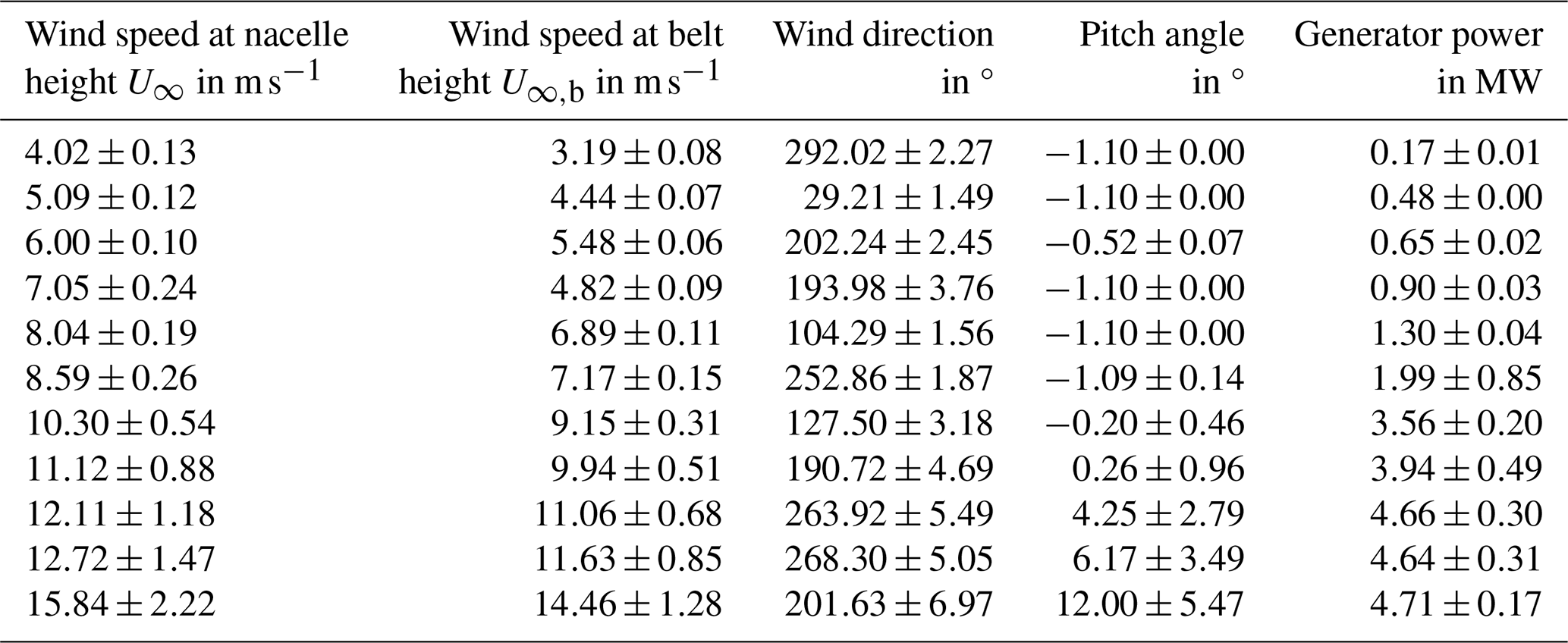
Since no wind speed measurements were available at the height of the pressure belt, wind speed values were interpolated to this level using vertical wind profiles. For each 10 min interval, a power-law wind profile was fitted based on the anemometer measurements at 33 and 90 m on the meteorological mast. The wind speed at the belt height, U_∞,b, was then interpolated from this power-law profile.

The orientation of the sensors with respect to the wind direction is shown in Fig. 4. Sensor data were aligned based on the mean wind direction, which is defined as 0°, indicating the direction from which the wind is coming. Sensors are then represented with their sensor angle β within a range of −180 to 180°. The negative side corresponds to the side facing the approaching rotor blade and is referred to as the blade-facing side. The positive side, which faces in the direction of rotor rotation, is referred to as the blade-opposing side.

The raw differential pressure data were converted into non-dimensional pressure coefficients C_p to enable comparison across varying wind conditions and sensor positions. The pressure coefficients were calculated using the interpolated wind speed at belt height U_∞,b:

$$\begin{array}{}\text{(1)}& C_p={\displaystyle \frac{p-p_{\mathrm{\infty }}}{\frac{\mathrm{1}}{\mathrm{2}}\mathit{\rho }{U}_{\mathrm{\infty },\mathrm{b}}^{\mathrm{2}}}}.\end{array}$$

The pressure coefficient was calculated based on the sensor output, defined as $p-p_{\mathrm{\infty }}=p_{\mathrm{out}}-p_{\mathrm{in}}$. Air density ρ was determined using the air pressure and temperature measured at the meteorological mast. Since the reference pressure inside the tower was not recorded, a correction was applied to the pressure distribution. Based on the wind direction, the sensor closest to the inflow direction (0°), i.e., closest to the stagnation point, was identified and its C_p value was set to 1. The pressure coefficients of all other sensors were then corrected by the corresponding offset.

4 Results and discussion

In Sect. 4.1 to 4.3, the results of the high-resolution pressure measurements obtained with the pressure belt are presented. This is followed by an analysis of the pressure belt long-term measurement data (Sect. 4.4). Finally, Sect. 4.5 examines the influence of the rotor–tower interaction on the rotor blade.

4.1 Tower flow field

In this section, flow phenomena such as velocity excess, stagnation point displacement, and pressure fluctuations around the tower, as predicted by Gómez and Seume (2009a), are analyzed and discussed.

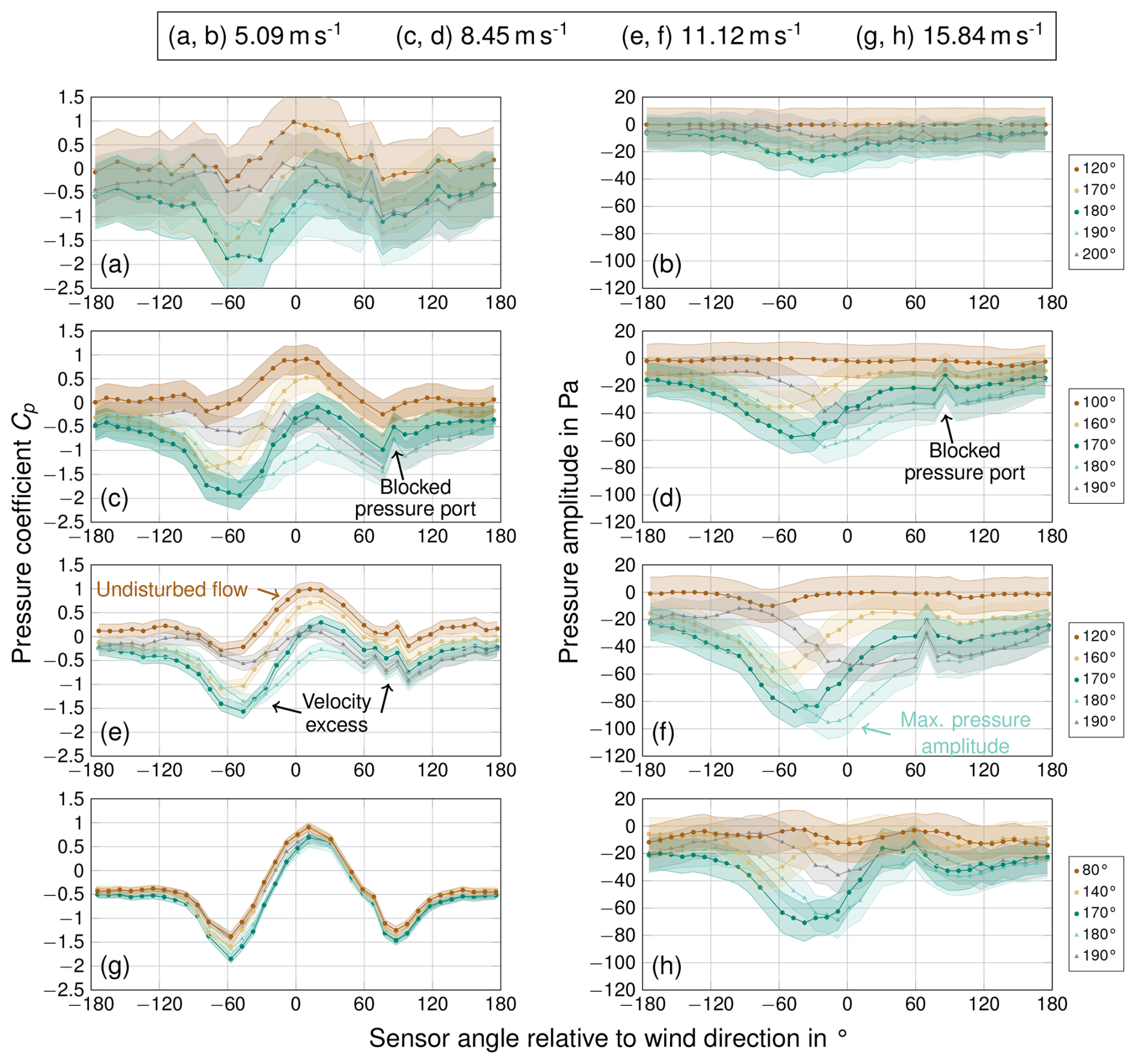
Figure 7 Left column: C_p distribution relative to wind direction. Right column: pressure amplitude relative to wind direction. The pressure amplitude is calculated as the difference between the current value of each sensor and its maximum over one rotor revolution. The colored curves represent the distributions at the corresponding rotor positions indicated in the legends (see Fig. 2 for definition of rotor position). Each row corresponds to a different wind speed. The shaded areas indicate the measurement uncertainty in the 95 % confidence interval.

4.1.1 Velocity excess

Figure 7 shows the measured C_p distribution (left column) and the corresponding pressure amplitude (right column) relative to the wind direction for selected rotor positions, covering a complete blade passage. Using the rotor position signal from the wind turbine, the pressure data were divided into 2° rotor position bins, and the mean value was calculated for each bin over the whole 10 min window. The different curves represent selected rotor positions. The pressure amplitude is the difference between the maximum mean value of each sensor over the full rotor revolution and the mean value at the current rotor position.

In the measurements represented by the brown curve, no rotor blade is located in front of the tower. It is observed for all wind speeds that the C_p values around the whole tower decrease as a rotor blade passes by. This trend is also reflected in the pressure amplitudes. Since the C_p value is directly related to the local flow velocity (a decreasing C_p corresponds to an increasing velocity), it becomes evident that the passing blade induces a flow acceleration at the tower surface. As the rotor blade approaches, the flow accelerates on the blade-facing side (negative angles) of the tower (represented by the yellow and green curves). As the blade has moved past the tower (gray curve), the flow on the blade-opposing side accelerates, while deceleration occurs on the blade-facing side. Across all wind speed ranges, the highest flow velocity (i.e., lowest C_p value) is consistently reached on the blade-facing side of the tower (green curves), which contrasts with the simulations by Gómez and Seume (2009a) and Shkara et al. (2018), where the strongest accelerations occur on the blade-opposing side.

When no rotor blade is located in front of the tower (brown curve), the C_p distribution is comparable to that of an undisturbed flow around a cylinder with the stagnation point in the middle. The C_p values at the flanks typically drop below −2 in this Reynolds number range of $\mathit{Re}=\mathrm{1.3}\mathrm{\dots }\mathrm{4.3}\times {\mathrm{10}}^{\mathrm{6}}$ (Jones et al., 1969). The fact that the C_p values at the flanks do not drop below −0.5 in the measurement of the undisturbed state indicates a deceleration of the flow caused by the pressure belt itself. This is also supported by the fact that, at higher wind velocities (Fig. 7g), the C_p values on the flanks of the undisturbed state become lower and the C_p distribution more closely resembles that of an undisturbed flow around a cylinder. In this case, the wind speed is sufficient to overcome the aerodynamic resistance introduced by the belt. An additional source of uncertainty arises from the reference wind speed, which was interpolated from measurements at the met mast upstream of the turbine. This approach does not account for possible changes in the flow between the met mast and the turbine or for the deceleration of the flow downstream of the rotor plane. It is also evident that the maximum pressure fluctuations reach only about 100 Pa (Fig. 7f), indicating an overall relatively low pressure fluctuation at this position on the tower.

Outliers can be observed in some of the C_p and pressure distributions (Fig. 7c and d). In these cases, the sensor signal appears to be damped, as indicated by a significantly lower amplitude compared to neighboring sensors. This indicates that the pressure fluctuations are not fully transmitted to the sensor, which is likely caused by a blocked pressure port due to moisture or debris.

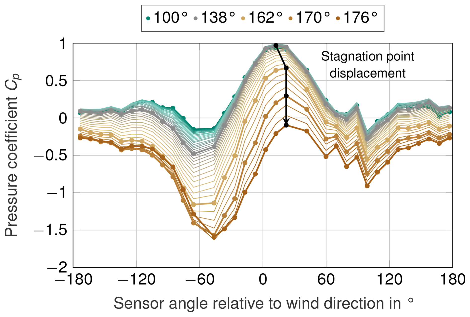
Figure 8 Mean C_p distribution in 2° increments of the rotor position as the blade approaches the tower. Curves corresponding to selected rotor positions are highlighted in bold and shown in the legend.

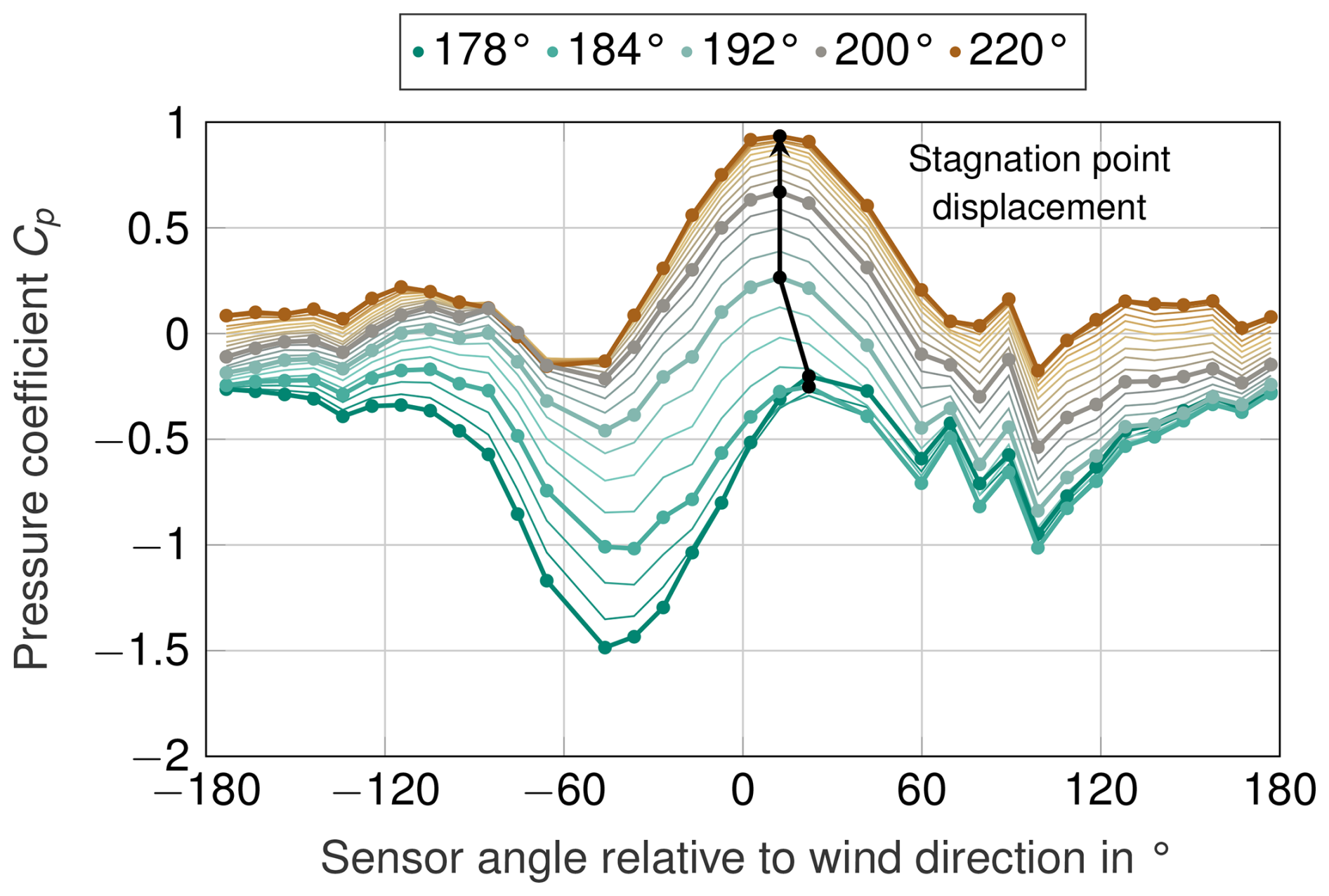
Figure 9 Mean C_p distribution in 2° increments of the rotor position as the blade moves away from the tower. Curves corresponding to selected rotor positions are highlighted in bold and shown in the legend.

4.1.2 Stagnation point displacement

Figures 8 and 9 show the mean C_p distribution for every 2° of rotor position during a single blade passage. Figure 8 shows the period during which the rotor blade approaches the tower (100° $\le \text{rotor position}\le \mathrm{176}$°), while Fig. 9 shows the period during which the blade moves away from the tower (178° $\le \text{rotor position}\le \mathrm{220}$°). Curves corresponding to selected rotor positions are highlighted in bold and are shown in the legend.

As previously noted in Sect. 4.1.1, a significant decrease in C_p values is observed on the blade-facing side (negative sensor angles), whereas the C_p values on the blade-opposing side show a less pronounced drop. The curves in Fig. 8 are closer to each other than in Fig. 9. This shows that the acceleration of the flow induced by the approaching blade occurs over a longer duration, whereas the deceleration and recovery of the flow toward the non-disturbed flow around the tower happen more rapidly.

A noticeable drop in C_p is also observed at the stagnation point. The maximum C_p value of each individual curve is marked in black. It can be seen that the stagnation point shifts by one sensor position (approximately 10°) in the positive direction of the sensor angle and, thus, toward the blade-opposing side. This indicates a slight stagnation point displacement, which was already found by Gómez and Seume (2009b). However, in the measurement, the drop in C_p near the stagnation point is significantly more pronounced. At a rotor position of 176°, the C_p value at the stagnation point is nearly equal to that on the backside of the tower, indicating a strong acceleration of the flow along the front side of the tower. Shkara et al. (2018) observed a pressure drop at the stagnation point in their simulations at rated power to values even lower than those on the back side of the tower. This behavior was only observed at a lower wind speed of 8.45 m s⁻¹ (Fig. 7c) in this study.

As previously observed, the rotor blade induces a velocity field around the tower: initially on the blade-facing side and, with increasing rotor position also on the blade-opposing side. This time-delayed, left-to-right progression of the induced velocity is superimposed on the potential flow of the undisturbed cylinder. As a result, the stagnation point is slightly displaced, and the flow in this region is additionally accelerated.

4.1.3 Wake skewness

The wake of a cylinder typically appears in the C_p distribution as a plateau on the backside, beginning at approximately ±120° in this Reynolds number range (Hau, 2016; Sørensen, 2009). A deflection of the wake would be expected to shift this plateau. However, such a shift is not clearly visible in the C_p distributions (Fig. 7). Instead, a general decrease in C_p and, thus, a pressure loss due to the flow separation is seen across the entire backside of the tower. Similarly to the stagnation point displacement, any deflection of the wake likely occurs over only a few degrees and is therefore impossible to resolve due to the sensor spacing.

4.2 Aerodynamic loading of the tower

The velocity induced by the passing rotor blade changes the pressure distribution around the tower and thus affects the aerodynamic loading of the tower. To characterize these effects, the drag coefficient c_d and lift coefficient c_l are evaluated over a full rotor revolution. These coefficients are calculated from the pressure coefficient C_p (Eq. 1) and the sensor angle β (Fig. 4) as follows:

$$\begin{array}{}\text{(2)}& {\displaystyle }{c}_l& {\displaystyle }=-{\displaystyle \frac{\mathrm{1}}{\mathrm{2}}}\underset{\mathrm{0}}{\overset{\mathrm{2}\mathit{\pi }}{\int }}{C}_p\sin \left(\mathit{\beta }\right)\mathrm{d}\mathit{\beta },\text{(3)}& {\displaystyle }{c}_d& {\displaystyle }={\displaystyle \frac{\mathrm{1}}{\mathrm{2}}}\underset{\mathrm{0}}{\overset{\mathrm{2}\mathit{\pi }}{\int }}{C}_p\cos \left(\mathit{\beta }\right)\mathrm{d}\mathit{\beta }.\end{array}$$

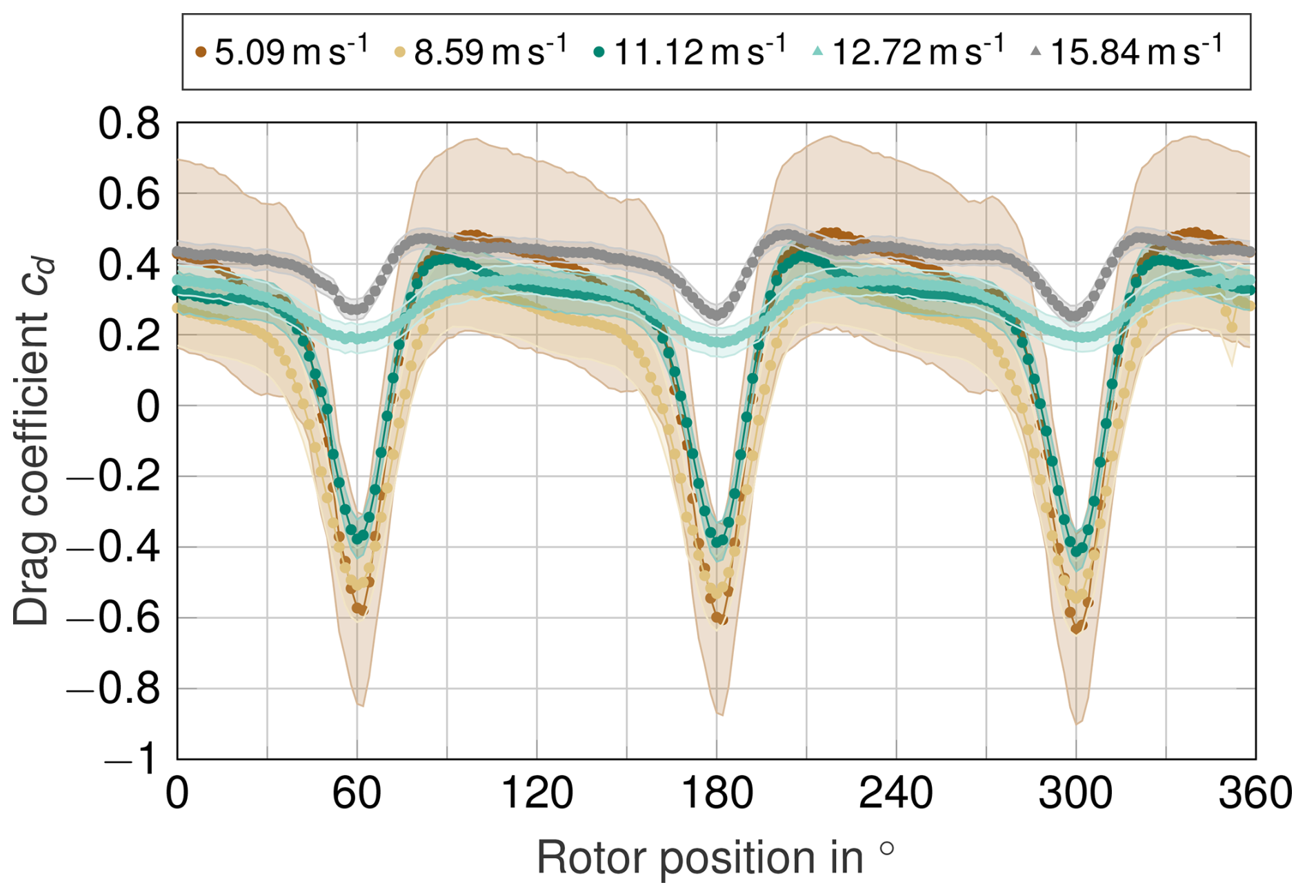
Figure 10 Drag coefficient of the tower as a function of rotor position. The different curves correspond to different wind speeds. The shaded areas indicate the measurement uncertainty in the 95 % confidence interval. The curves have been corrected for inconsistent rotor position timestamps and aligned so that the first pressure minimum appears at 60°.

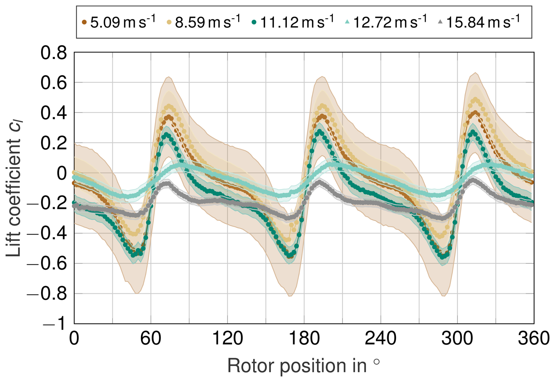
Figure 11 Lift coefficient of the tower as a function of rotor position. The different curves correspond to different wind speeds. The shaded areas indicate the measurement uncertainty in the 95 % confidence interval. The curves have been corrected for inconsistent rotor position timestamps and aligned so that the first pressure minimum appears at 60°.

Figure 10 shows the drag coefficient c_d as a function of the rotor position for four different wind speeds. It can be observed that c_d drops three times per rotor revolution. The highest values occur when no rotor blade is in front of the tower. A value of c_d≈0.4 in this state agrees well with the typical drag coefficient of a cylinder in this Reynolds number range (Hau, 2016).

A significant decrease in c_d is observed when a blade passes the tower. This fluctuation of the coefficients occurs mainly within an azimuthal range of approximately ±30° around the tower passage. A similar fast change was observed by Carrion et al. (2014) in their simulations of the NREL Phase VI turbine. At wind speeds up to 11.12 m s⁻¹, the minimum values even reach negative levels, as predicted by González (2010). When no blade is in front of the tower, the pressure distribution around the tower resulting from the flow field produces a net force that pushes the tower in the direction of the free stream, resulting in a positive c_d. When a blade passes in front of the tower, the flow on the front side of the tower is accelerated. This acceleration causes a pressure drop at the front, leading to a net force opposite to the free-stream direction and resulting in a negative c_d. At wind speeds of 12.72 and 15.84 m s⁻¹, c_d remains positive throughout the entire rotor revolution, indicating that the tower is continuously loaded in the direction of the free flow.

Due to inconsistent rotor position timestamps between each examined operating point, the curves were aligned by shifting them so that the first pressure minimum of each curve coincides at 60° rotor position. This corresponds to the rotor position at which the first rotor blade passes the tower and ensures consistent phase alignment across all analyzed operating points.

Figure 11 shows the lift coefficient c_l as a function of the rotor position. A positive c_l indicates a force component acting in the direction of rotor rotation, i.e., toward the blade-opposing side of the tower. A clear 3P periodic fluctuation is observed as well, with c_l initially decreasing into the negative range and subsequently rising into the positive range. As the blade approaches the tower, a higher flow velocity on the blade-facing side of the tower is induced, leading to a local pressure drop and a net force acting in that direction. As the blade moves past the tower, the pressure on the blade-facing side increases again, while it decreases on the opposite side. This shift in the pressure distribution results in a lateral force acting in the opposite direction.

It is noticeable that some curves do not oscillate symmetrically around c_l=0, indicating a slight asymmetry in lateral loading. The coefficient values are referenced to the wind direction measured at the meteorological mast. Possible causes for this offset are a constant cross flow induced by the rotor blade, a deviation of the local inflow direction at the turbine, or a combination of both effects.

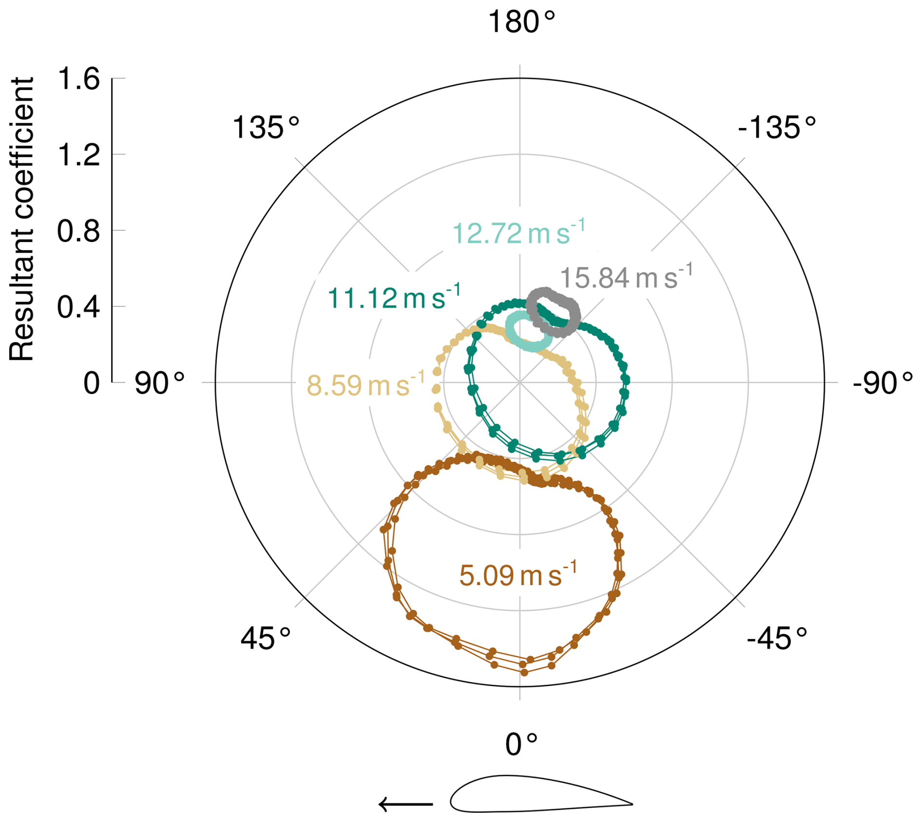
Figure 12 Mean resultant force coefficient plotted against the corresponding angle relative to the free-stream direction (see Fig. 4 for angle definition). Different curves correspond to different wind speeds.

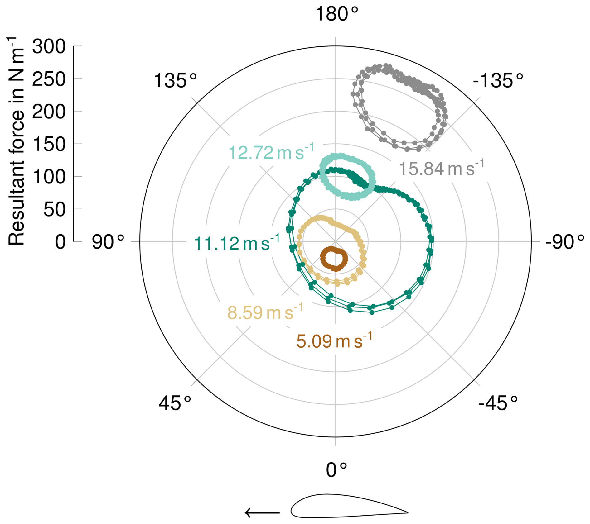
Figure 13 Mean resultant force plotted against the corresponding angle relative to the free-stream direction (see Fig. 4 for angle definition). Different curves correspond to different wind speeds.

From the axial and lateral loads acting simultaneously on the tower, the resulting load on the tower can be determined. Figure 12 shows the mean value of the resultant force coefficient c_R and the corresponding angle β^′ for different wind speeds. The resultant force coefficient and its corresponding angle are calculated as follows:

$$\begin{array}{}\text{(4)}& {\displaystyle }{c}_{\mathrm{R}}& {\displaystyle }=\sqrt{c_{\mathrm{l}}^{\mathrm{2}}+c_{\mathrm{d}}^{\mathrm{2}}},\text{(5)}& {\displaystyle }{\mathit{\beta }}^{\prime }& {\displaystyle }=\arctan \left({\displaystyle \frac{c_{\mathrm{l}}}{c_{\mathrm{d}}}}\right).\end{array}$$

The resultant force coefficient over a complete rotor revolution occurs now as a circle in the polar diagram. When the circle is centered around the coordinate origin (e.g., at 8.59 and 11.12 m s⁻¹), this indicates that the resultant force completes a full rotation during a single blade passage. As a result, the tower is subjected to a circumferential load, with the magnitude of the force varying with the angle.

For very low and very high wind speeds, the tower experiences loading predominantly in a single principal direction. At higher wind speeds (12.72 and 15.84 m s⁻¹), the pressure fluctuations induced by the blade are small relative to the dynamic pressure of the free flow, resulting in a net load acting only in the direction of the free flow (0°). At 5.09 m s⁻¹, the tower is consistently loaded opposite to the flow direction over the entire rotor revolution. It is possible that, at this wind speed, only the flow on the front side of the tower is significantly influenced by the rotor blade. Since the dynamic pressure is still relatively low, this may also be a measurement artifact caused by the pressure belt itself. The blade-influenced flow might not carry enough energy to fully overcome the surface roughness of the belt, which slows down the flow. As a result, the sensors on the backside of the tower detect a distorted flow velocity. Overall, the relative contribution of the fluctuating pressure component decreases with increasing wind speed, as indicated by the decreasing circle diameters at higher wind speeds.

The resultant force acting on the tower can be estimated using the mean wind speed at belt height U_∞,b and the tower diameter D_tow with the following equation:

$$\begin{array}{}\text{(6)}& F_{\mathrm{R}}={\displaystyle \frac{\mathrm{1}}{\mathrm{2}}}\mathit{\rho }{U}_{\mathrm{\infty },\mathrm{b}}^{\mathrm{2}}{D}_{\mathrm{tow}}{c}_{\mathrm{R}}.\end{array}$$

This result can be seen in Fig. 13. The largest force fluctuation, which is identified by the diameter of the largest circle in the polar plot, occurs at a wind speed of 11.12 m s⁻¹. The gray circle is furthest out, which means that the highest average force value occurs at a wind speed of 15.84 m s⁻¹. As already noted, the static load on the tower increases with rising wind speed. The rotor blade superimposes this load with a dynamic fluctuation, which is most pronounced at a wind speed of 11.12 m s⁻¹. And as the wind speed continues to rise, the effect of this dynamic fluctuation decreases compared to the static loading caused by the free flow.

The maximum range of the coefficients and the resulting force across all investigated operating points are determined by identifying the largest diameter of the circles in Figs. 12 and 13. The results are shown in Figs. 14 and 15. The coefficient range is initially high and then decreases significantly between 10 and 12 m s⁻¹. In this wind speed range, the force range also shows a notable decline. By comparing with Table 1, it becomes evident that the force amplitude increases with rising wind speed as long as the blades are not pitched. At 12 m s⁻¹, the pitch angle becomes positive, and the blades are pitched out of the wind. In this region, both the force and coefficient amplitudes decrease.

The maximum dynamic aerodynamic loading on the tower occurs just as the turbine reaches rated power. At this operating point, the aerodynamic forces on the blade are strongest, and, due to blade bending, the blade–tower clearance is at its minimum. This results in the greatest aerodynamic interaction between blade and tower and, consequently, the highest dynamic loading on the tower. As the wind velocity increases further, the rotor blades are pitched out of the wind, resulting in a larger clearance and a reduction in dynamic loading on the tower. Figure 15 shows that, at the operating point of 15.84 m s⁻¹, after the drop between 10 and 13 m s⁻¹, the force amplitude increases again. Since the aerodynamic forces on the rotor blade are already decreasing at this wind velocity, it is likely that a blade-shadowing effect occurs. The passing rotor blade intermittently disrupts the high free-stream velocity, leading to fluctuating loads on the tower.

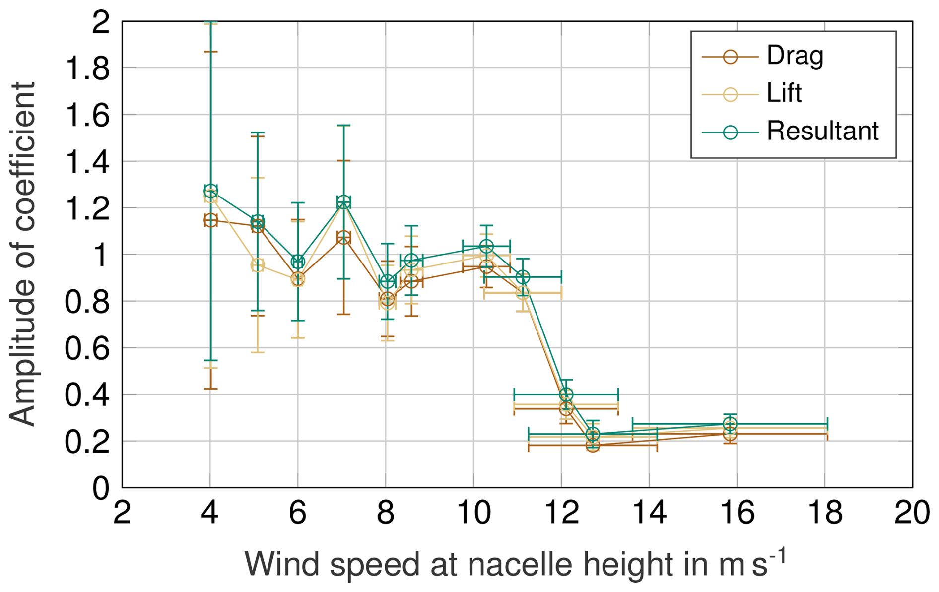
Figure 14 Maximum amplitude of the resultant force coefficient (corresponding to the maximum diameter of the curves in Fig. 12) as a function of the free-stream velocity. Results are shown for all operating points listed in Table 1. The vertical error bars indicate the measurement uncertainty in the 95 % confidence interval. The horizontal error bars represent the standard deviation of the 10 min average wind velocity.

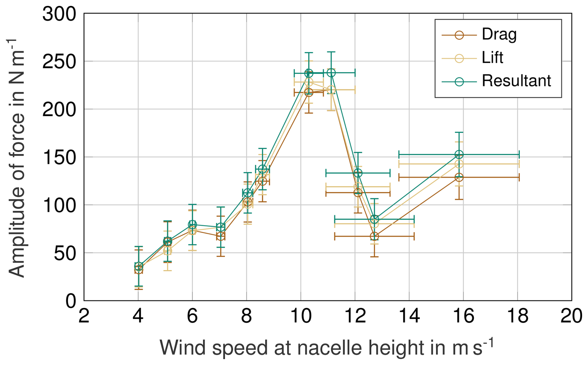
Figure 15 Maximum amplitude of the resultant force (corresponding to the maximum diameter of the curves in Fig. 13) as a function of the free-stream velocity. Results are shown for all operating points listed in Table 1. The vertical error bars indicate the measurement uncertainty in the 95 % confidence interval. The horizontal error bars represent the standard deviation of the 10 min average wind velocity.

4.3 Frequency domain

Figures 16 and 17 show the order-based FFT (fast Fourier transform) analysis of the drag and lift coefficients. It is clearly visible that both coefficients exhibit distinct peaks at the 3P frequency and its higher harmonics (6P, 9P, 12P, etc.). This confirms that the tower loading is strongly driven by the aerodynamic influence of the rotor blades.

The peak at 1.44P corresponds to the tower vortex shedding synchronized with the blade passage, as previously predicted by Gómez and Seume (2009b). This effect is most pronounced at a wind speed of 11.12 m s⁻¹, which is the operating point where the rotor–tower interaction is strongest.

Figure 16 Order-based FFT analysis of the drag coefficient.

Figure 17 Order-based FFT analysis of the lift coefficient.

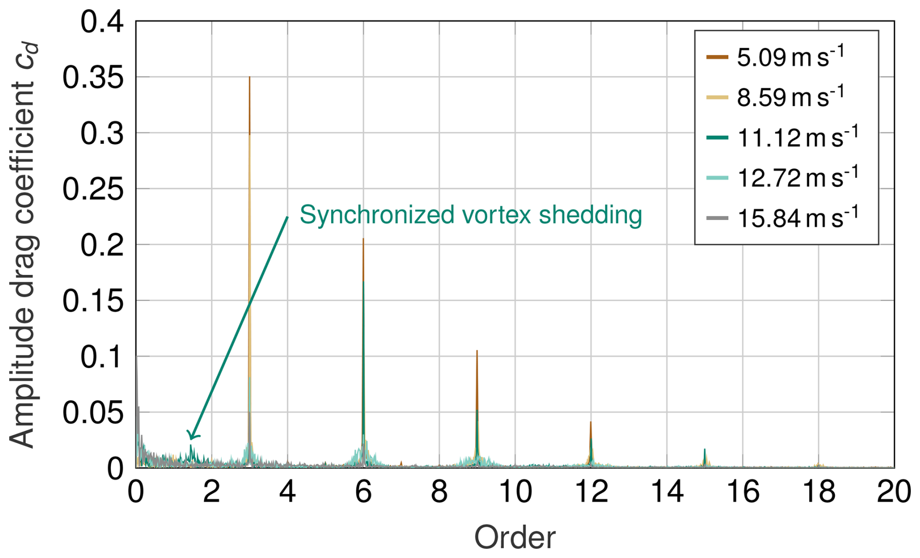
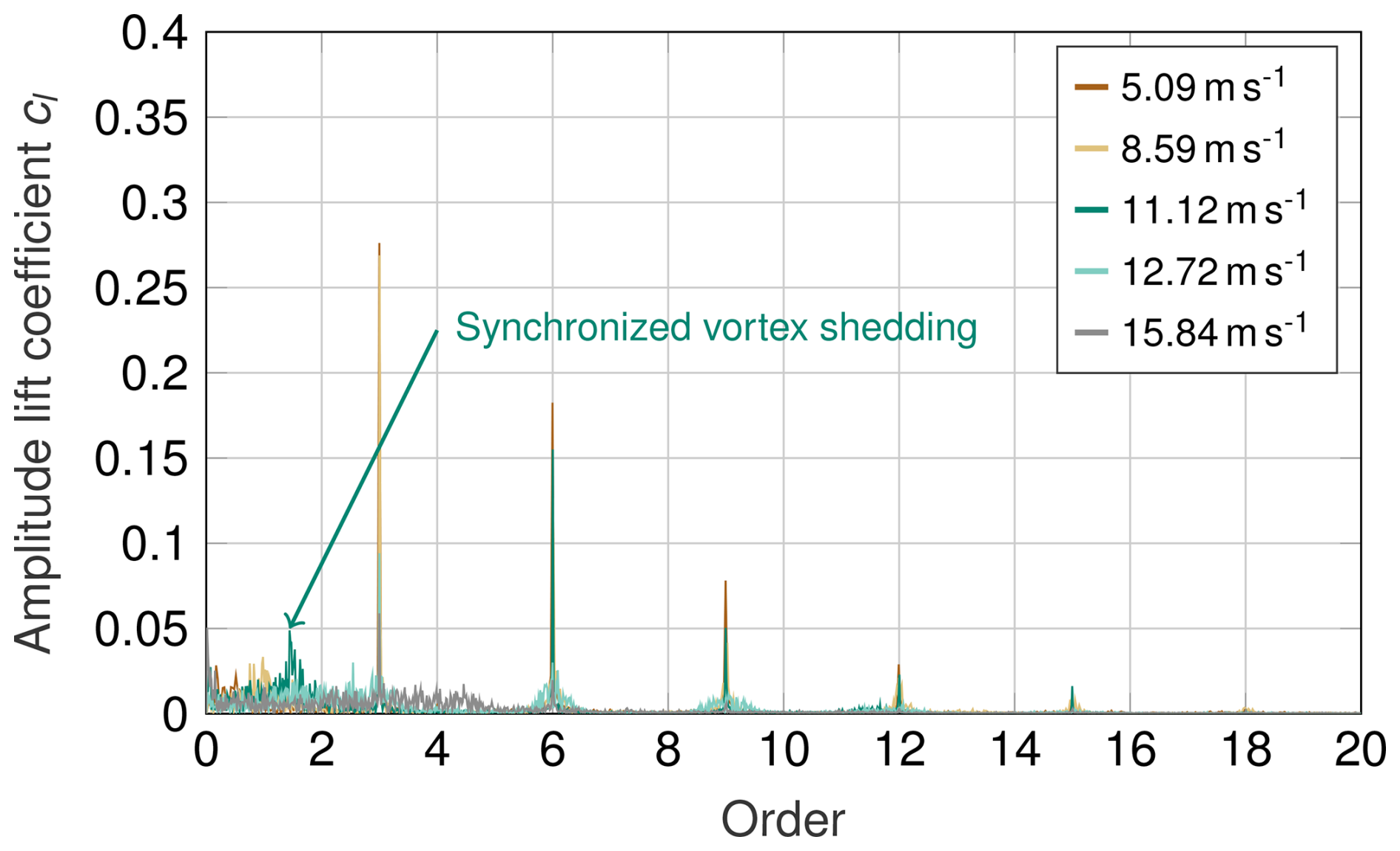
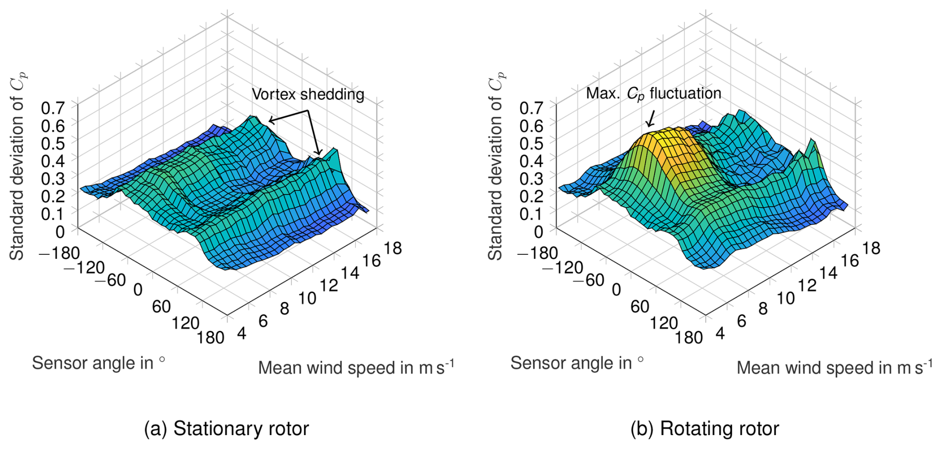
Figure 18 The 1 min averages of the standard deviation of C_p as a function of sensor angle relative to the wind direction (see Fig. 4 for angle definition) and wind speed. (a) Stationary rotor, when no blade is in front of the tower. (b) Rotating rotor.

Figure 19 The 1 min averages of the standard deviation of pressure p as a function of sensor angle relative to the wind direction (see Fig. 4 for angle definition) and wind speed. (a) Stationary rotor, when no blade is in front of the tower. (b) Rotating rotor.

4.4 Long-term measurement data

In this section, 1 min averaged data over the entire measurement period are analyzed to support the previously presented findings. The aim is to confirm the observed phenomena within the context of a long-term analysis. The measured fluctuations for both the non-rotating and rotating rotor are analyzed. Figure 18a shows the standard deviation of C_p as a function of the sensor angle relative to the wind direction and wind speed for the non-rotating rotor. Two distinct ridges appear to the left and right of 0°, corresponding to the vortex shedding of the tower. Under rotating-rotor conditions (Fig. 18b), a significant increase in C_p fluctuation is observed on the blade-facing side. The two vortex-shedding ridges are still visible, indicating that vortex shedding continues to occur and, as shown in Sect. 4.3, is synchronized with the blade-passing frequency. It is clearly visible that the maximum C_p fluctuations on the tower surface occur as the turbine reaches rated power, which is consistent with the previous findings.

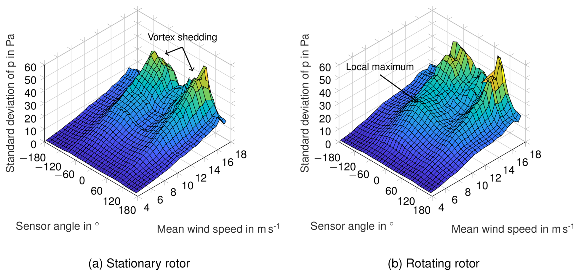
Figure 19 shows the standard deviation of the pressure fluctuations. The two ridges associated with vortex shedding are clearly visible again. For the rotating rotor, a local maximum in pressure fluctuations is observed at rated power. Beyond this point, the pressure fluctuations continue to increase and become significantly larger at higher wind speeds. This observation is consistent with the findings in Sect. 4.2 and suggests that, in this wind velocity regime, because the aerodynamic loading of the blade is already decreasing, the pressure fluctuations are caused by the blade interrupting the free-stream flow.

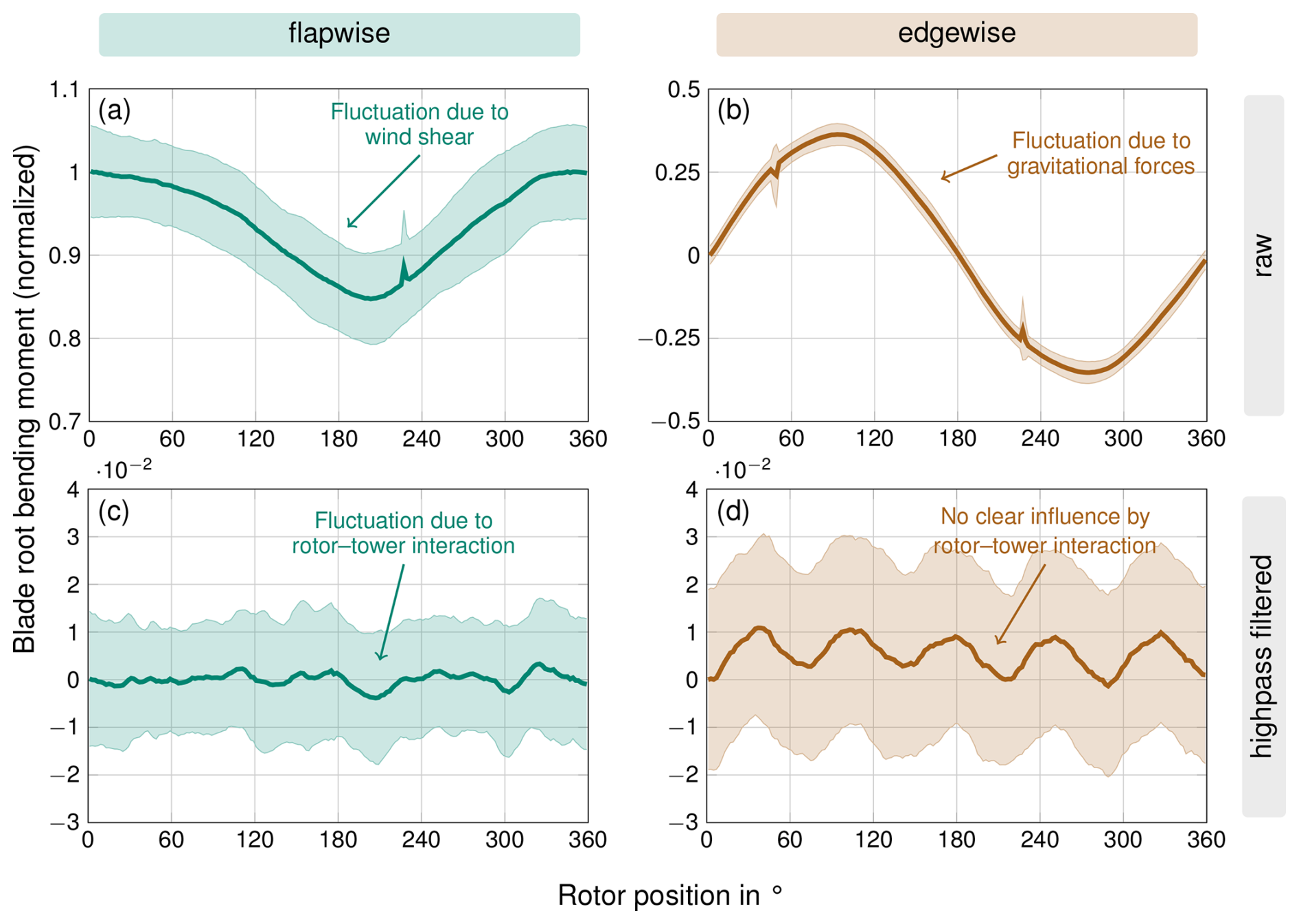
Figure 20 Flapwise (left column) and edgewise (right column) root bending moments of one rotor blade as a function of rotor position for the operating point $U_{\mathrm{\infty }}=\mathrm{11.12}\mathrm{m}{\mathrm{s}}^{-\mathrm{1}}$ (Table 1). The top row shows the raw signal, while the bottom row shows the high-pass-filtered signal. For confidentiality reasons, the data were normalized to the maximum flapwise bending moment. The shaded areas indicate the standard deviation of the 10 min average.

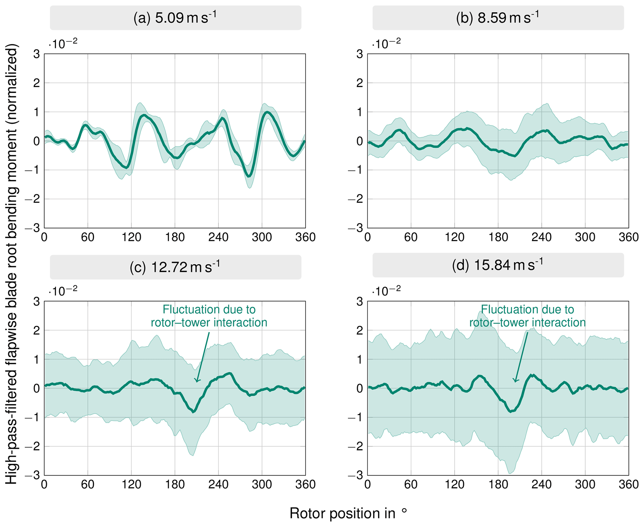
Figure 21 High-pass-filtered flapwise bending moment as a function of rotor position for selected operating points from Table 1. For confidentiality reasons, the data were normalized to the maximum flapwise bending moment at the operating point $U_{\mathrm{\infty }}=\mathrm{11.12}\mathrm{m}{\mathrm{s}}^{-\mathrm{1}}$ (Fig. 20a). The shaded areas indicate the standard deviation of the 10 min average.

4.5 Influence on the rotor blade

González (2010) derived theoretically that the rotor blade and tower influence each other aerodynamically. Since the previous sections have demonstrated that the tower is affected by the rotor blade, the following section investigates whether the blade is also influenced by the presence of the tower. Figures 20a and 20b show the flapwise and edgewise bending moments at a wind speed of 11.12 m s⁻¹, the condition under which the aerodynamic loading on the blade is highest and effects on the blade due to rotor–tower interaction are most likely to be observed. At a rotor position of 200°, the blade has just passed the tower. A distinct change in the flapwise bending moment is observed at this rotor position, whereas no noticeable change appears in the edgewise bending moment. A delayed occurrence of the minimum flapwise blade loading after the blade has passed the tower was also reported by Carrion et al. (2014). The 1P fluctuation of the flapwise bending moment caused by wind shear is clearly visible. Since both wind shear and rotor–tower interaction introduce 1P loads, the changes in bending moment resulting from the rotor–tower interaction cannot be distinctly identified through an FFT analysis of the bending-moment signal. This was one of the reasons why uniform inflow conditions were selected for the NREL Phase VI turbine experiments in order to better isolate and distinguish the individual effects (Hand et al., 2001).

Assuming that the tower's influence on the blade occurs as an impulsive load during the blade's passage through the disturbed tower flow field, the signal is instead high-pass filtered using a Butterworth filter to reveal the effect of rotor–tower interaction on the blade (Fig. 20c and d). A cut-off frequency equal to 4 times the rotor's rotational frequency was selected for the high-pass filter. In the flapwise bending moment, a fluctuation is now visible during the tower passage. In contrast, no noticeable influence is observed in the edgewise bending moment, and it is therefore not analyzed further.

The high-pass-filtered flapwise bending moments for various wind speeds are shown in Fig. 21. At low wind speeds, no clear influence of the tower is visible (Fig. 21a and b). However, at higher wind speeds (Fig. 21c and d), the influence of the tower becomes visible. Considering the amplitude in Fig. 21c, this fluctuation accounts for approximately 1 % of the maximum flapwise bending moment, which is lower than the values reported by Shkara et al. (2018), Shkara et al. (2020), Kim et al. (2011), and Ghandour et al. (2022). Together with the relatively low pressure fluctuations identified earlier, this indicates that rotor–tower interaction appears to be relatively weak for the investigated turbine type when compared to a large portion of the published literature.

The numerical studies in the literature show different assessments of the strength of rotor–tower interaction, depending on the applied modeling assumptions. The low interaction strength observed in this study suggests that some simulation-based predictions for modern upwind turbines may overestimate rotor–tower interaction effects if simplified inflow conditions or simplified structural models are used. A closer comparison of the studies reporting the lowest interaction amplitudes reveals that these conclusions were obtained under different modeling approaches. Shkara et al. (2020) considered wind shear and a flexible turbine model based on the NREL 5 MW reference turbine, whereas Zahle and Sørensen (2008) employed a rigid structural model without tilt but used geometric and operational data of an actual Siemens multi-megawatt turbine. This comparison highlights that similar quantitative outcomes can arise from different modeling assumptions. In this context, it is noteworthy that the turbine investigated in the present study features a tilt angle of 7°, a configuration not explicitly considered in the referenced literature, to the best of the authors' knowledge. With increasingly realistic simulation setups that account for structural flexibility, wind shear, tilt, and turbine-specific geometry, the magnitude of predicted rotor–tower interaction effects may converge toward the lower amplitudes measured in this study. This could in turn indicate potential for optimizing the distance between rotor blades and tower in future upwind turbine designs. To conduct a robust assessment, the turbine would need to be monitored over a longer period, and the most severe wind conditions, such as the strongest gusts in low wind shear, would need to be identified during rated operation. Under these conditions, the blade–tower clearance could then be re-evaluated.

Even though the contribution is small, rotor–tower interaction adds to the fatigue loading of the rotor blades of modern multi-megawatt wind turbines. The remaining question is how significant this contribution is. For the present analysis, operating points with the lowest wind speed fluctuations were selected for each wind speed bin from a total measurement period of approximately 2 months. To determine the share of rotor–tower interaction in the overall fatigue loading more precisely, a broader evaluation covering the full wind speed and turbulence spectrum is required. Nevertheless, the effect is significantly smaller than that observed for similarly sized downwind turbines (Bortolotti et al., 2025), which underlines the advantage of upwind turbine configurations in this respect.

5 Conclusions

Although rotor–tower interaction is generally less pronounced in upwind wind turbines compared to downwind configurations, it is still measurable under real operating conditions. A pressure belt proved to be a suitable instrumentation for experimentally investigating the effects caused by rotor–tower interaction on a multi-megawatt wind turbine.

The strongest dynamic loading on the tower due to rotor–tower interaction was observed at rated power, where the aerodynamic forces on the rotor blades are highest. As wind speed increases beyond this point, the tower is subjected to increasing static loads from the free-stream wind, while the relative contribution of dynamic pressure fluctuations decreases. Overall, rotor–tower interaction appears to be relatively weak in this turbine type as the maximum measured pressure amplitudes at the tower were around ±100 Pa. Deviations of the bending moment at the blade root of approximately 1 % caused by rotor–tower interaction were also smaller than those reported by Shkara et al. (2018, 2020), Kim et al. (2011), and Ghandour et al. (2022). Nevertheless, the aerodynamic phenomena, such as velocity excess and stagnation point displacement, which were predicted by Gómez and Seume (2009b); Gomez and Seume (2009), could be confirmed in this study. This shows that the interaction between the rotor and the tower influences the flow field around the tower and that the underlying theoretical considerations accurately predict these effects.

Because the pressure fluctuations at low wind speeds were close to the sensor's specified uncertainty of ±50 Pa, the pressure sensors had to be recalibrated. It was found that the Amsys AMS 4712-0050-D-B sensors all had individual offsets and were able to resolve fluctuations in the range of ±7.3 Pa (95 % confidence interval). Due to the small pressure amplitudes, especially at low wind speeds, the pressure belt itself may have influenced the flow around the tower. In future experiments, a redesigned belt should therefore be used that is thin enough to only minimally disturb the flow around the tower. A narrower spacing of pressure ports could help to resolve the stagnation point displacement more precisely. This setup can be complemented by a pressure belt mounted on the rotor blade at the same height as the tower-mounted belt. This will allow a simultaneous investigation and comparison of the local flow around both the tower and the rotor blade.

The presented results raise the question of whether future multi-megawatt wind turbines could be designed with reduced tower clearance. To address this question, the investigated turbine would need to be analyzed over a longer observation period and under the most unfavorable wind conditions. In this context, the digital image correlation (DIC) measurements can provide additional insight. The rotor blades of the investigated turbine are also equipped with DIC markers so that the deformation of the blades can be measured during operation. The gained data can be used to quantify the blade–tower clearance and to investigate the blade deformation during tower passage. However, even studies in the literature reporting stronger rotor–tower interaction effects did not observe any blade–tower contact. This suggests that current blade–tower clearance requirements for modern multi-megawatt wind turbines may be conservative, with potential for reduced clearances.

Overall, this study demonstrates that rotor–tower interaction occurs in a modern multi-megawatt wind turbine and can be measured under real operating conditions. The primary contribution of this study is therefore methodological, providing a field demonstration of the applied measurement approach. In future work, a broader evaluation of the available measurement data and accompanying CFD simulations are required to further substantiate the findings.