Influence of the inflow conditions on the dynamics of a floating wind turbine wake under harmonic surge motion

Floating offshore wind turbines (FOWTs) are projected to undergo substantial expansion in the coming decades. However, the high compliance of their floating foundations, coupled with aerodynamic, hydrodynamic and mooring forces, leads to complex platform motions that make it difficult to predict their wake dynamics. The vortex ring structure produced during surge motion has been the subject of study for nearly a decade now but there are still many features to bring to light. As most studies have been under idealised uniform flow, there is little knowledge on how this structure behaves under atmospheric boundary layer (ABL) flow. In this work, the authors propose to study this structure under three different inflow conditions: laminar and low-turbulence no-shear flows and ABL flow. Large eddy simulations are carried out in combination with an actuator disc (AD) as a wind turbine model, with a focus on surge motion and a Strouhal number ranging between 0 and 0.47. The velocity values are extracted at a vertical plane parallel to the AD axis, which is subsequently analysed by means of proper orthogonal decomposition (POD) and phase averaging. In the POD analysis, vortex ring structures are identified under all inflow conditions, though their energy decreases as turbulence increases. Additionally, a dependence of energy on frequency is observed for low-turbulence no-shear and ABL flows, with the maximum energy occurring at Strouhal numbers 0.30 and 0.32, respectively. Furthermore, vertical meandering is detected in both cases. In low-turbulence no-shear flow, meandering and vortex rings act as decoupled phenomena. Replicating the analysis on a horizontal plane at hub height, it is observed that lateral meandering is uniformly intense under this inflow condition. Conversely, under ABL conditions, the surge motion interacts with the turbulent shear flow to actively induce a coupled vertical meandering. Vertical and lateral meandering in ABL conditions rely on entirely distinct mechanisms, the latter being unrelated to the vortex ring structure. Finally, phase-averaging analysis indicates that the wake is modulated by the surge motion, manifesting as expansions and contractions, for laminar and low-turbulence no-shear cases. Conversely, an inclination of the structures towards the flow direction is identified in the ABL conditions, attributable to the shear flow.

1 Introduction

In the global pathway towards decarbonisation, wind energy has become one of the leading renewable technologies over the past decades. As shallow-water sites become increasingly saturated, floating offshore wind turbines (FOWTs) are expected to play a central role in the expansion of wind power into deeper waters (Zhou et al., 2025). However, the knowledge gained from bottom fixed wind turbines still leaves several open questions when extrapolated to floating configurations, since in addition to aerodynamics, hydrodynamics and mooring now also play a significant role. FOWTs are subjected to rigid-body motions in six degrees of freedom, which lead to an overall modification in both aerodynamic performance and the wake structure formed downwind. It was first described by Xu et al. (2015), Farrugia et al. (2016), Tran and Kim (2016) and Wen et al. (2017) that wind turbines subjected to periodic surge movement show oscillations in thrust and power output, as the blades experience variations in the local angle of attack. Schulz et al. (2024) state that these oscillations can be considered a superposition of quasi-steady effects caused by the instantaneous changes in the apparent wind speed experienced by the moving rotor and the impact of potential unsteady aerodynamic phenomena. Also, it has been pointed out that, out of all possible movements, wind turbine aerodynamics are mostly affected by turbine surge and pitch motions (Lee and Lee, 2019; Wang et al., 2023). In terms of wake modifications, surge motions generate a pulsating mode in the form of periodic expansion and contraction in the wake, which have been studied for the past decade both numerically and experimentally (Sivalingam et al., 2018; Messmer et al., 2024; Hubert et al., 2025).

In the numerical modelling of FOWT wakes, simulations using an actuator line model (ALM) have consistently shown that surge motion induces a transformation of standard helical tip vortices into distinct stronger vortex ring structures (Arabgolarcheh et al., 2023a, b; Wang et al., 2024). The formation and strength of these structures are heavily dictated by the platform's motion frequency, which directly governs the growth rate of vortex instabilities (Kleine et al., 2022). As demonstrated by Duan et al. (2022) using blade-resolved improved delayed detached eddy simulation (IDDES), the surge frequency governs the intensification of these vortex rings at specific intervals and has a significantly larger impact on the overall wake structure than the surge amplitude. While ALM and blade-resolved approaches are strictly necessary to resolve the discrete transient helical tip vortices in the near-wake, the actuator disc (AD) model presents a highly suitable and computationally efficient alternative for studying the overall wake behaviour under surge motion. Although the AD approach inherently bypasses the resolution of individual blade tip vortices, it successfully captures the downstream symmetric vortex ring structures that dominate the interaction between surge motion and wake development. As pointed out by Kopperstad et al. (2020), the inherent symmetry of these rings makes the AD particularly appropriate for such far-wake analyses. This assumption is further substantiated by recent ALM studies (Zhou et al., 2025) which confirm that vortex rings formed under surge motion firmly retain their symmetry. Furthermore, the AD method has been reliably applied to demonstrate how surge-induced turbulence accelerates wake recovery (Rezaeiha and Micallef, 2021), thereby justifying its application for evaluating overall wake development under surge motion.

However, most of the aforementioned studies characterising these surge-induced structures were carried out under uniform idealised flow conditions. This is a useful approach to isolate the particular phenomena present in FOWT but it leaves out effects produced in atmospheric boundary layer (ABL) flow. In particular, due to the continuously increasing size of wind turbines, there is a need for studies that can predict the effect of ABL flow over the vortex ring structure. Also, ABL turbulence is responsible for wake meandering, which interacts with the wake dynamics produced by surge motion. For these reasons, Xu et al. (2022) suggest the need for further investigations of more realistic atmospheric inflows and strong interactions between multi-FOWTs. In this line of work, Zhou et al. (2022) and Nybø et al. (2022) studied the effect of atmospheric turbulence on FOWT by means of synthetic turbulence generators, and in the case of Nybø et al. (2022) the results were compared with large eddy simulations (LES), pointing out that synthetic models may lead to incorrect estimations for FOWT dynamic responses besides not considering ABL flow thermal stability. Johlas et al. (2019, 2020) conducted full ABL simulations incorporating the motions induced by waves on an ALM. The results demonstrated that, due to turbine pitch motion, the wakes of FOWTs exhibit an upward deflection in comparison to the wakes of fixed wind turbines. Also, Xu et al. (2023, 2024) studied full ABL flows combined with ALM by means of LES in the first case and DDES (delayed detached eddy simulation) in the second. Results confirm previous findings for wake centre deflection under pitch motion and that, under ABL flow, platform motions have negligible impact on wake recovery. The latest work also includes a comparison with uniform and shear flows. In terms of vortex structures, they were able to visualise the tip vortices breaking apart into the ring structure for the uniform and shear cases but, due to the presence of other structures in ABL flow, the ring vortex structure is not distinguished in the wake for this case. Bridging this specific gap, namely understanding the persistence and behaviour of vortex rings generated by surge motion under realistic atmospheric turbulence and shear, constitutes the primary motivation of the present study.

Regarding the experimental approach, Messmer et al. (2024) studied a model wind turbine under laminar flow and surge motion, analysing a range of Strouhal numbers $\mathit{St}=\frac{f_{\text{surge}}D}{U_{\text{ref}}}$ between 0 and 1, where D denotes the disc diameter, f_surge the surge motion frequency and U_ref the upstream reference velocity. Results show a clear pulsating structure on the wake for $\mathrm{0.2}\le \mathit{St}\le \mathrm{0.55}$, with the frequency of the motion appearing in the wake spectra. In terms of realistic inflow conditions, Schliffke et al. (2020, 2024) conducted experiments in an ABL wind tunnel with a porous disc subjected to surge motion and analysed the wake profile at 4.6 D downstream. These experiments included a range of $\mathrm{0}\le \mathit{St}\le \mathrm{0.36}$. The authors observed that while harmonic motions leave a clear frequency signature in the wake's energy spectra, they do not significantly alter time-averaged statistics. Specifically, for a motion amplitude of $\frac{D}{\mathrm{8}}$, in the second work they determined that a St number of at least 0.19 was required to detect this signature at a downstream distance of 8 D, as almost no sign is detected for St≤0.13. Also, the higher signature was observed close to St=0.30. In the context of the UNAFLOW campaign, Fontanella et al. (2021, 2022b) obtained analogous results regarding wake recovery by analysing the wake at 2.3 D under uniform inflow conditions with low TI. Recently, Hubert et al. (2025) investigated the spatio-temporal nature of this effect achieving an experimental visualisation of the signature of the vortex ring structure under ABL flow by means of particle image velocimetry (PIV). Even at a lower Strouhal number (St=0.11), they described the wake's dynamic response as a pulsating behaviour, characterised by a periodic contraction and expansion of the wake rather than a displacement of its centre.

To successfully isolate these periodic structures from background turbulence, advanced analysis techniques are required. The proper orthogonal decomposition (POD) method provides a decomposition basis for the data that is optimal in terms of energy as it sorts the resulting modes by energy content. It is useful in cases where certain structures have a specific associated frequency (Iungo et al., 2015), like the case of the vortex ring structure and surge motion. In VerHulst and Meneveau (2014) Hamilton et al. (2018) and Ali et al. (2021) the method was applied to the wake obtained from LES combined with an AD, and in Andersen et al. (2014) and Cherubini et al. (2022) with an ALM. In the latter, the frequency spectrum was calculated for each mode to have a better interpretation of the structures present. Bastine et al. (2014, 2015) applied this method considering a plane at 4 D downstream an AD to visualise the modes under ABL flow. Regarding FOWT cases, Wang et al. (2024) applied the method downstream an ALM under surge motion and uniform inflow. The results show that four modes are enough to capture 95 % of the energy in the wake. Also, in Raibaudo et al. (2022) the technique was applied to planes of streamwise velocity obtained experimentally at 4.6 D and 8.1 D downstream a porous disc model under surge motion. For each case, the corresponding surge frequency was identified within the modes but no specific spatial mode was found.

As far as the authors are aware, there is still lack of studies that explain the effects of combining realistic ABL conditions with FOWT phenomena. In this work, we expect to shed some light on this matter by comparing the flow structures produced by surge motion under three distinct inflow conditions: laminar no-shear flow, low-turbulence no-shear flow and ABL flow, hereafter named laminar, low-turbulence and ABL cases, respectively. This progression allows us to systematically test the effects of background turbulence and vertical shear flow. LES are carried out together with an AD representing a FOWT model under surge motion. The numerical framework for the ABL case was configured following the experimental setup of Schliffke et al. (2024), enabling comparisons with the reported wake dynamics and spectral characteristics throughout the article. Different frequencies of surge motion are analysed, and the resulting wake for each case is studied using POD and phase averaging with the corresponding surge frequency. By applying these techniques, this study aims to characterise the spatial and temporal evolution of the pulsating structures and determine how they are modulated or disrupted by the atmospheric environment.

The paper will be organised as follows: the numerical setup is detailed in Sect. 2. Section 3 presents the mesh sensitivity analysis and baseline wake flow characterisation. Then, the POD analysis is outlined in Sect. 4, followed by the phase average study in Sect. 5. Finally, conclusions are drawn in Sect. 6.

2 Numerical setup

The numerical setup is defined based on the wind tunnel located at École Centrale Nantes, where porous discs have been studied as wind turbine models for the past years under an offshore-like ABL flow (Schliffke et al., 2020; Belvasi et al., 2022; Schliffke et al., 2024; Hubert et al., 2025). With a 26 m test section and a cross section measuring 2 m by 2 m, this open-circuit atmospheric wind tunnel is set up to reproduce a neutral atmospheric boundary layer at a geometric scale of 1:500. The porous disc diameter is 0.16 m, resulting in a blockage ratio of approximately 0.5 %, and in the case of ABL flow, the hub height is 0.12 m. While the present study adopts the same geometric scale, inlet profiles and motion parameters as the experimental campaigns, its objective is not to perform a direct quantitative validation against a specific dataset. Instead, the experimental configuration is used as a physically realistic and well-characterised reference framework to isolate and analyse the fundamental wake dynamics under controlled inflow conditions.

Within this framework, three different inflow conditions are considered. The first one is a uniform laminar flow where the inlet velocity is unperturbed. Then, a second case is built with a perturbation on the inlet flow leading to a uniform low-turbulence flow, with a TI≈1.2 %. Finally, an ABL flow is considered with a higher turbulence, reaching TI≈9 % at hub height. The mean velocity and turbulence intensity profiles will be presented in Sect. 3. In the case of the ABL flow, the results presented herein build upon and substantially extend the preliminary findings reported in Barile et al. (2025). Through these three varying inflows, specific phenomenological similarities with the experimental observations are qualitatively compared later in Sects. 4 and 5.

2.1 Numerical model

The flow is governed by the spatially filtered incompressible Navier–Stokes equations, which are solved using the SOWFA libraries (NREL, 2012; Churchfield et al., 2012a, b) within the OpenFOAM framework (OpenCFD-Ltd, 2004). The subgrid-scale stresses are modelled using a one-equation eddy viscosity approach (Yoshizawa, 1986) for the ABL case and a Smagorinsky formulation for the laminar and low-turbulence cases. The AD forces are included as source terms in the momentum equations.

While the core numerical framework follows the standard SOWFA implementation, two main modifications were introduced to suit the current study. First, temperature variations were disregarded, focusing solely on the fluid mechanical behaviour of the flow. Second, the driving mechanisms were adapted depending on the flow case. ABL flow simulations are driven by a forced pressure gradient. For this case, a precursor region is defined upstream of the AD where a specific reference velocity is forced at hub height. Only the average velocity at hub height in this region is taken into account to calculate the pressure gradient, which is then applied to the entire domain. This approach ensures that the forcing mechanism is not biased by the local flow perturbations induced downstream the disc while still maintaining the desired boundary-layer development. Conversely, the laminar and low-turbulence flow simulations are driven by an inlet boundary condition instead of a pressure gradient. In both cases, the same reference velocity value is set. However, in the low-turbulence case, a perturbation is added to achieve a low-turbulence inflow with length scales close to the ABL case, as described in Sect. 2.3. In contrast, an unperturbed inflow is considered for the laminar case.

2.2 Actuator disc

To represent the effect of the porous disc an AD approach (Jimenez et al., 2007; Mikkelsen, 2004) is used, which is similar to the one presented in Navarro Diaz et al. (2019a, b, 2021). The AD is represented by a set of nodes arranged on a planar disc that are independent of the background fluid mesh. Nodes are arranged as rings and the separation between rings is set according to Navarro Diaz et al. (2023). To ensure numerical stability, the nodal forces are later spread to the surrounding cells through a regularisation kernel, which relies on a three-dimensional Gaussian distribution (Porté-Agel et al., 2011; Hodgson et al., 2021).

First, a calibration table is constructed, for which the motionless AD is simulated with different fixed inlet wind speeds and uniform force distribution, in order to establish the induction relation between the unperturbed wind speed and the velocity at each AD node. During the computational fluid dynamics (CFD) simulation, the AD is subjected to a sinusoidal surge motion where the position and velocity are given by

$$\begin{array}{}\text{(1)}& {\displaystyle }\mathrm{\Delta }x\left(t\right)=A_{\text{surge}}\sin \left(\mathrm{2}\mathit{\pi }{f}_{\text{surge}}t\right),\text{(2)}& {\displaystyle }\mathrm{\Delta }v\left(t\right)=\mathrm{2}\mathit{\pi }{f}_{\text{surge}}{A}_{\text{surge}}\cos \left(\mathrm{2}\mathit{\pi }{f}_{\text{surge}}t\right).\end{array}$$

In the above expressions, A_surge is the surge amplitude, which is considered $D/\mathrm{8}$ based on Schliffke et al. (2020, 2024) and f_surge the corresponding frequency, which differs across cases. Considering the fluid velocity at each node U_i, the local velocity sensed by the AD node is obtained in each time step as

$$\begin{array}{}\text{(3)}& U_{i|\mathrm{rel}}\left(t\right)=U_i\left(t\right)-\mathrm{\Delta }v\left(t\right)\end{array}$$

which is then used to enter the calibration table and obtain the unperturbed wind speed relative to the AD, U_∞|rel. Finally, the force is calculated as

$$\begin{array}{}\text{(4)}& \mathrm{\Delta }{f}_i={\displaystyle \frac{\mathrm{1}}{\mathrm{2}}}\mathit{\rho }{C}_{\mathrm{t}}{U_{\mathrm{\infty }|\mathrm{rel}}}^{\mathrm{2}}\mathrm{\Delta }{S}_i,\end{array}$$

where ρ is the air density, C_t is the disc thrust coefficient and ΔS_i is the area corresponding to the particular AD node. The thrust coefficient of the AD is set to C_T=0.65 to match the experimental measurements of the porous disc (Aubrun et al., 2019). This value is kept constant under platform surge motion. Although the platform motion induces variations in the apparent inflow velocity of approximately ±25 % relative to the upstream velocity, the corresponding Reynolds number changes do not significantly affect the aerodynamic drag characteristics of the rigid porous mesh, as previously verified experimentally for varying inflow speeds (Aubrun et al., 2019).

While this constant C_T approach accurately replicates the passive aerodynamic behaviour of a physical porous disc undergoing surge motion, it introduces a loss of generality when extending the results to a real three-bladed wind turbine rotor. In a physical floating wind turbine, the instantaneous thrust coefficient varies due to changes in tip-speed ratio, pitch control actions and dynamic inflow effects induced by the platform motion. Consequently, the present AD framework isolates the purely kinematic interaction between the surge motion and the wake dynamics, serving as a fundamental baseline for more complex aeroelastic scenarios.

2.3 Computational domain and boundary conditions

In the case of laminar and low-turbulence flows, a 25 D long domain is built, with a 10 D × 10 D cross section. This cross-sectional area yields a blockage ratio of less than 1 %. Since this value is well below the typical 5 % threshold where confinement effects become significant (Sarlak et al., 2016), the numerical domain is wide enough to avoid artificial acceleration around the AD. The starting mesh is uniform and various mesh refinements are carried out. In order to capture the surge motion, a higher resolution is required. Therefore, the cells near the AD are twice as large in the cross directions as they are in the flow direction. To carry out a mesh convergence study, four meshes are built under these conditions and compared for the case of a motionless AD under laminar flow, analysing the wake at 4 D, 6 D and 8 D downstream the AD. The characteristics of the four meshes are presented in Table 1 and mesh no. 2 is shown in Fig. 1. This mesh contains 12.8 cells D⁻¹ in the cross direction and 25.6 cells D⁻¹ in the flow direction and is the one selected for the rest of the study, as will be shown in Sect. 3. Also, the chosen mesh leaves 8 D upstream the AD inside the more refined mesh in order to give the flow enough space to develop correctly before arriving at the AD. Finally, 12 D are left behind with the same cell size to cover the wake from 2 D till 10 D.

Table 1 Details about the meshes analysed during the mesh convergence study for laminar flow.

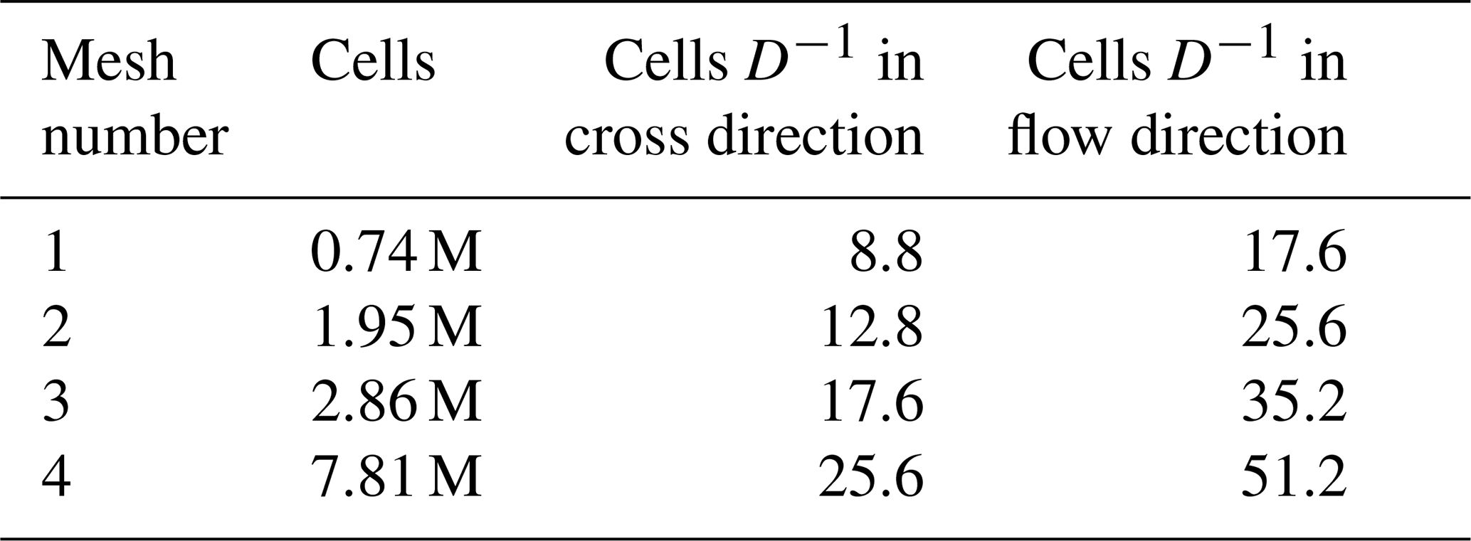
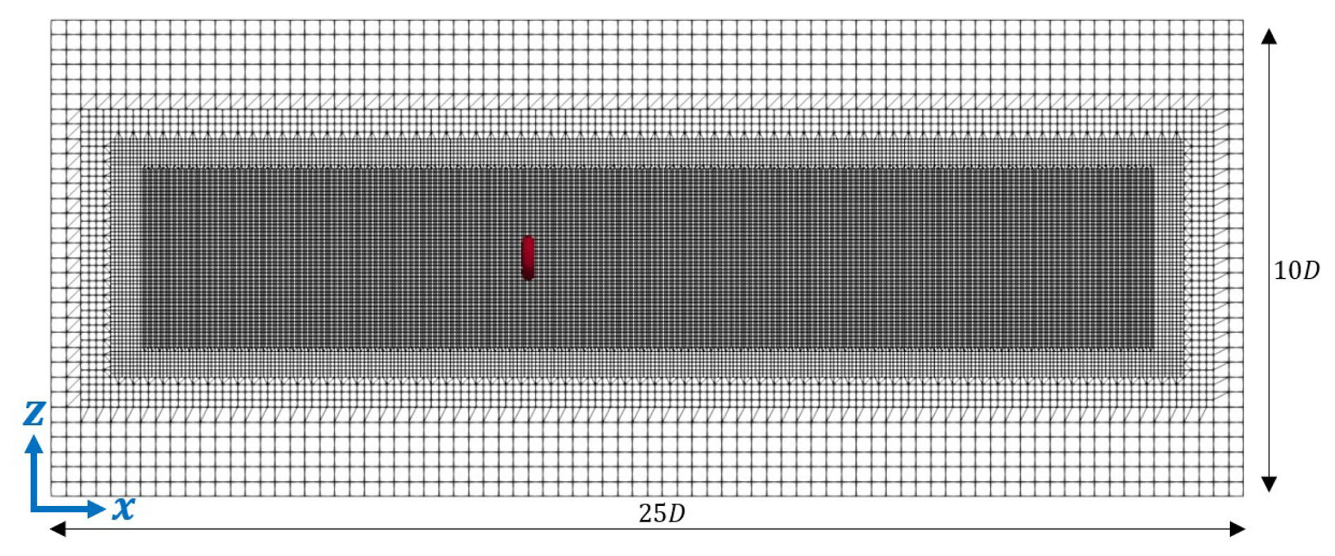
Figure 1 Schematic of the mesh implemented for laminar and low-turbulence flow cases. 8 D and 12 D are left upstream and downstream, respectively, with the smallest cells.

To achieve a converged ABL flow, many authors have opted for the precursor technique, where the flow is developed by recirculation until convergence, and only then it is presented with the wind farm (Churchfield et al., 2012a, b; Stevens et al., 2014; Lanzilao and Meyers, 2023). In this work, the authors choose to include the precursor region within the simulation domain, as it is done by Chen et al. (2022), and the inlet is set by mapping the end of the precursor region. The zone of analysis is located downstream this region. A schematic of the numerical domain is shown in Fig. 2, where the flow at 75 D from the inlet is mapped into the domain inlet boundary condition (BC). For the ABL case, the domain dimensions are 175 D long and 10 D wide, but the height is reduced to 5 D. This cross section yields a blockage ratio of approximately 1.5 %, which, similarly to the uniform flow cases, is well below the 5 % threshold, ensuring that confinement effects remain negligible. The decision to restrict the domain height is intrinsically linked to the numerical modelling of the atmospheric surface layer (ASL). At the real scale, the ASL refers to the lowest portion of the ABL where turbulent quantities and fluxes display a near-constant behaviour (Richards and Hoxey, 1993; Stull, 2012; van der Laan et al., 2020, 2021). Simulating a deep domain for a neutrally stratified ABL without resolving temperature gradients, and thus lacking an inversion capping layer, can lead to an artificial decay of turbulence in the upper portion of the domain. To avoid this issue in the present scaled configuration, the domain height is limited to 5 D. This reduced height is combined with a top stress boundary condition, which provides the required forcing to maintain realistic turbulence levels and preserve a consistent ASL profile over the downstream distance considered (Zahn and Bou-Zeid, 2024). The mesh originally contains 12.8 cells D⁻¹ in the vertical direction and 3.2 cells D⁻¹ in the horizontal direction. Also, a mesh height gradient is imposed near the bottom in order to correctly model the flow near the surface, and the same gradient is applied near the top. After the precursor region, based on the previously mentioned mesh convergence study, two mesh refinements are carried out only in the horizontal direction, reaching 25.6 cells D⁻¹ in the region near the AD for both horizontal directions and 12.8 cells D⁻¹ in the vertical direction. This mesh refinement continues up to 25 D downstream the AD. The resulting total number of cells is 4.84 M.

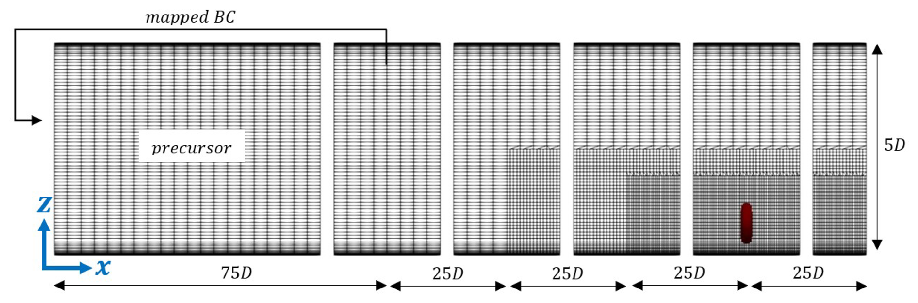
Figure 2 Schematic of the mesh implemented for ABL flow. After the precursor region, two mesh refinements are carried out in the horizontal direction.

Cyclic lateral BCs are imposed in all cases. For the laminar and low-turbulence cases, the other two boundaries (top and bottom) are set to slip. For the ABL case, stress boundary conditions are prescribed at both faces to sustain the neutral ASL. The bottom boundary follows Schumann’s model (Schumann, 1975) to account for the physical surface roughness of the wind tunnel floor, while the top boundary applies a shear-stress condition based on the target friction velocity u^*, similar to what is done by Jimenez et al. (2007) and Zahn and Bou-Zeid (2024). The inlet boundary condition is set to a velocity fixed value without any perturbation in the laminar case, while a filtered noise boundary condition is applied for the low-turbulence case. This type of inflow, as originally proposed by Klein et al. (2003), consists of imposing the desired length scales on a random Gaussian white noise through a filtering operation and subsequently scaling to achieve the desired Reynolds stress tensor. Following this, the targeted mean flow is superimposed on the signal. For the low-turbulence case, the targeted mean flow is entirely uniform (i.e. it contains no vertical shear) and only the turbulent fluctuations are superimposed. For further details regarding this process, we refer the reader to Immer (2016). The turbulent length scales used for the filtering process in the inlet flow are set equal to the values obtained in the ABL flow, but the same length scale is set in both cross directions. In order to achieve an average uniform flow with a lower turbulence, the same values are specified in the entire inlet surface. Regarding the physical characteristics of the chosen ABL, it is modelled to represent the scaled wind tunnel boundary layer experimentally studied by Schliffke et al. (2024) rather than a specific physical site. Accordingly, the target velocity and turbulence intensity profiles were configured following VDI guideline 3783 (VDI, 2000) for atmospheric boundary layer wind tunnel modelling. This provides a standardised, strongly sheared and highly turbulent baseline to contrast with the uniform inflow cases without shear.

2.4 Cases analysed

Table 2 summarises the cases analysed in this work. The reference velocity U_ref=2.71 m s⁻¹ is taken at the inlet for the uniform flow cases and at the AD original position in a simulation without AD for the ABL case. The specific test cases are selected following those in Schliffke et al. (2020, 2024), whose experimental setup was originally designed to replicate the Floatgen project, featuring a 2 MW Vestas V80 wind turbine with a 60 m hub height and an 80 m rotor diameter.

Table 2 Surge frequency of the cases analysed in this work with the corresponding Strouhal number. In all cases, the amplitude is set to $\frac{D}{\mathrm{8}}$.

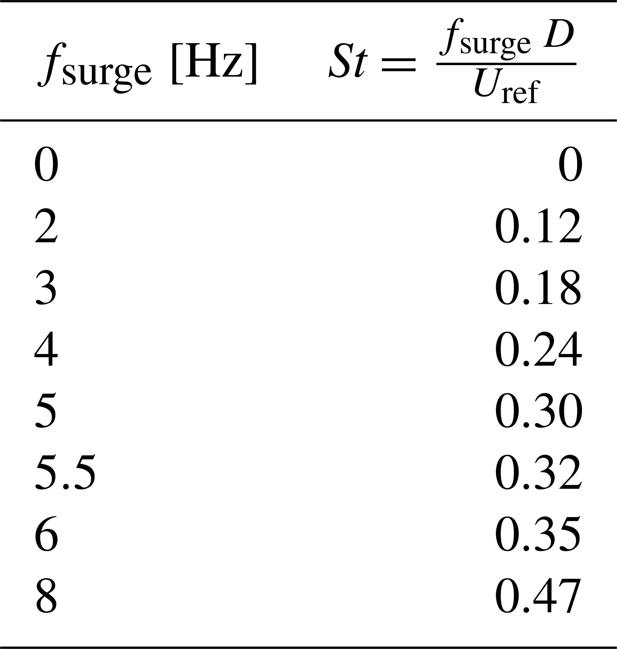
Although these initial experiments were scaled based on a 2 MW turbine, the selected Strouhal numbers hold direct physical relevance to modern 10 to 15 MW floating wind turbines. For such full-scale turbines, characterised by rotor diameters of 180 to 240 m and near rated wind speeds of approximately 10 to 11 m s⁻¹ (Zahle et al., 2014; Gaertner et al., 2020), the St range of 0.12 to 0.47 corresponds to physical oscillation frequencies between 0.005 and 0.03 Hz. This frequency range is representative of the rigid-body platform motions typically observed in spar and semisubmersible floating wind turbines, whose natural frequencies generally lie between approximately 0.005 and 0.05 Hz for large-scale systems (Allen et al., 2020; Fontanella et al., 2022a). Specifically, a motion amplitude of $\frac{D}{\mathrm{8}}$ represents a bounding scenario for extreme resonant responses in these large structures. Consequently, this study focuses strictly on these low-frequency, large-amplitude dynamics, whereas higher reduced frequencies (St>0.5), typically associated with first-order wave excitation, fall outside the current scope.

3 Mesh sensitivity analysis and wake flow characterisation

This section presents the preliminary results of the LES. First, a mesh convergence study is performed for the laminar inflow case to evaluate the accuracy of the numerical setup. Then, an independent assessment is carried out for the low-turbulence and ABL inflow cases, where the inflow generation method is validated against experimental inflow conditions for the latter. Finally, the vortex ring structure is analysed by examining the vorticity field and the Q criterion for one of the surge frequencies considered in this work.

In order to verify the mesh convergence, a laminar uniform flow inlet is applied to the four meshes described in Table 1, including the AD with no movement. The first 10 s are left for the flow to develop, after which the results of the following 40 s are averaged. Based on the time scaling factor of 150 associated with this experimental setup (Schliffke et al., 2024), these intervals translate to approximately 25 min of initialisation and 100 min of continuous data collection at full scale. The time-averaged velocity deficit profiles of all cases at 4 D, 6 D and 8 D downstream the AD are compared in Fig. 3a, b and c, respectively. It can be seen that mesh no. 2 already reaches convergence near the wake centre for the flow downstream the AD. This agreement with the finer meshes is maintained at 6 D and 8 D, where the profiles for mesh no. 2 show a consistent behaviour across the entire wake width, suggesting that the spatial resolution is adequate for the purposes of this study.

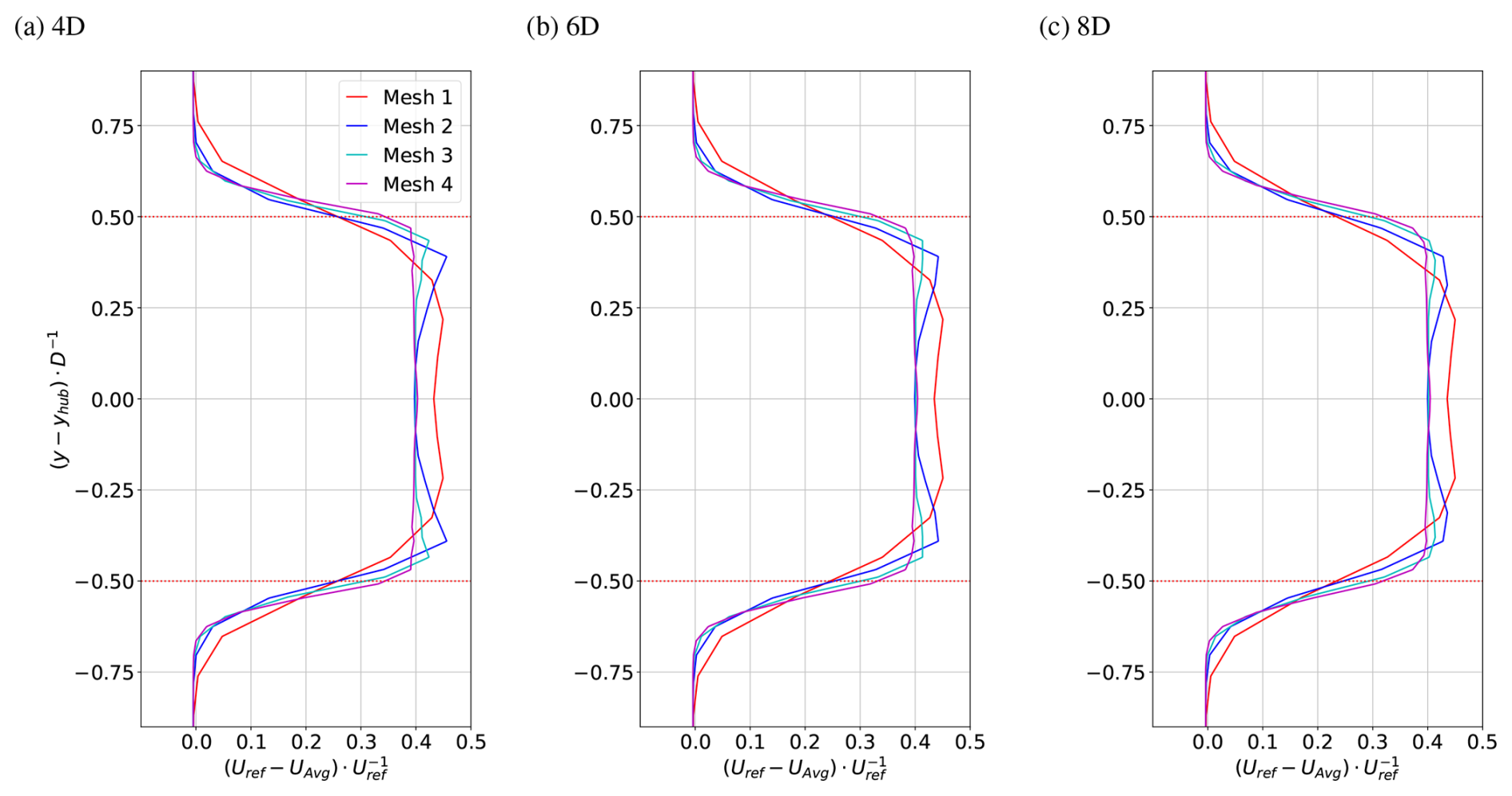
Figure 3 Average velocity deficit results for the mesh convergence study under laminar uniform flow at 4 D, 6 D and 8 D downstream the AD.

With regard to the low-turbulence inflow conditions, following mesh refinement, 10 s are allowed for the flow to develop in a simulation without the AD. Thereafter, two consecutive 40 s periods are run. Figure 4a presents the averaged velocity zoomed around the AD region during the second period, followed by the TI split into three components, in Fig. 4b, c and d. The initial plot displays a uniform inflow, while the subsequent three plots demonstrate statistical convergence of the flow during these specified periods. In such conditions, a turbulence intensity of approximately 1.2 % is obtained, and the integral length scale is found to be approximately $L_u^x\approx \mathrm{910}$ mm.

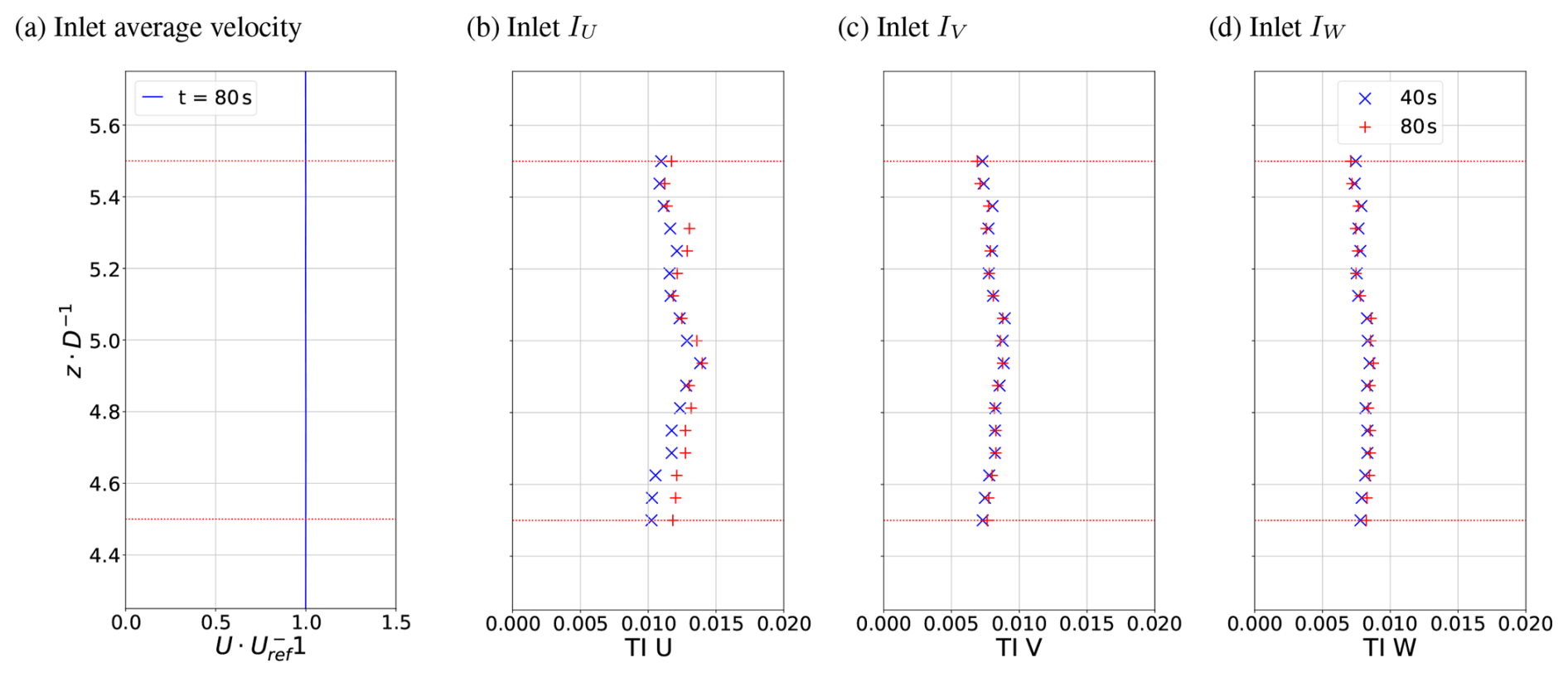
Figure 4 Inlet flow average velocity (a) and TI profiles for the three velocity components (b, c, d) after mesh refinement for low-turbulence flow. All profiles are zoomed in the refined region. The dotted red lines delimit the height of the porous disc.

In order to verify that the ABL wind tunnel profile is accurately reproduced during the simulations, an initial precursor stage is run for 1200 s on a base mesh without mesh refinement or AD. Using the resulting flow field as the initial condition, the two mesh refinements detailed in the previous section are carried out. The simulation is run for an additional 100 s (up to t=1300 s) to allow the flow to develop correctly before the results are recorded. A total of 80 s is then run, split into two runs of 40 s each. Based on the time scaling factor of 150 (Schliffke et al., 2024), these intervals correspond to 250 min of initialisation and 100 min per run at full scale. The results for the average velocity, zoomed in the AD region, after 80 s are shown in Fig. 5a along with the profile reported in Schliffke et al. (2024), which corresponds to a scaled maritime boundary layer, showing a high degree of correlation. Also, each component of the turbulence intensity for the two 40 s run is shown in Fig. 5b, c and d, which demonstrate statistical convergence between the two periods. The experimental values reported in Schliffke et al. (2024) are also included for comparison. Compared with these experimental values, the CFD exhibits a close match across all three components, with a slight surplus observed in the U component and a slight deficit in V and W components. In such conditions, a turbulence intensity of approximately 9 % is obtained at hub height, and the integral length scale at this point is found to be approximately $L_u^x\approx \mathrm{750}$ mm, which is of the same order of magnitude as the experimental value reported in Schliffke et al. (2024); Hubert et al. (2025), $L_u^x\approx \mathrm{480}$ mm. For the cases including the AD, the process is repeated, starting with the results of the first 1200 s. The AD is activated when the mesh refinements are carried out, and 100 s are left for the wake to develop.

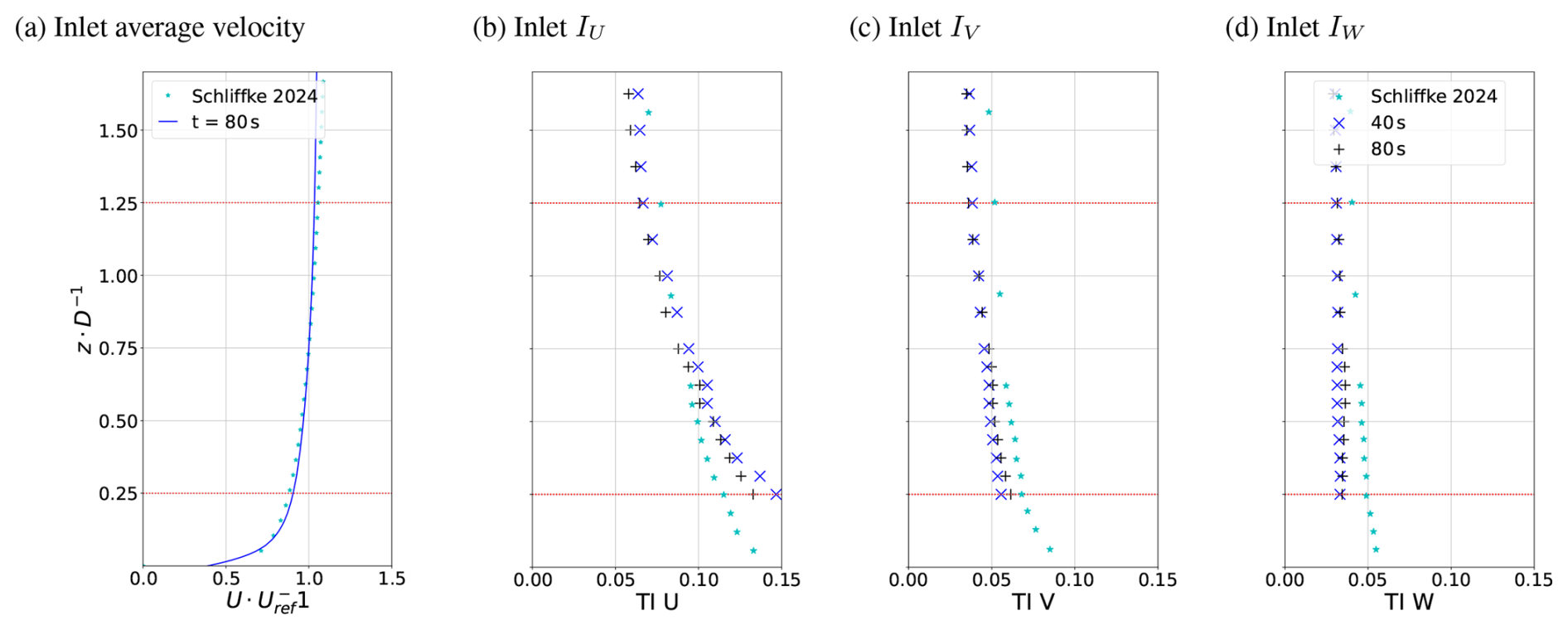
Figure 5 Inlet flow average velocity (a) and TI profiles for the three velocity components (b, c, d) after mesh refinement. All profiles are zoomed in the refined region and compared with experimental values from Schliffke et al. (2024). The dotted red lines delimit the height of the porous disc.

For the three inflow conditions (laminar, low-turbulence and ABL), the cases from Table 2 are simulated as described. Data recording starts at 10 s for the laminar and low-turbulence inflow cases and at 1300 s for the ABL inflow case. Two consecutive simulation periods of 40 s each are performed with the moving AD. In a first attempt to visualise the flow structure, Q criterion contours (Q=50) are presented for a harmonic surge motion at S_t=0.32 under laminar, low-turbulence and ABL flows in Fig. 6a, b and c, respectively. The figure clearly shows the vortex ring structure for both the laminar and low-turbulence inflow cases. This vortex ring structure was previously visualised under uniform inflow for a variety of St values: Arabgolarcheh et al. (2023b) for St=0.08 and 0.18, Duan et al. (2022) and Zhou et al. (2025) for St=0.55, Wang et al. (2024) for St=0.69 and Arabgolarcheh et al. (2023a) for St=1.22. In contrast, the ABL flow exhibits no clear structure in the wake. This was also the finding of Xu et al. (2024), in which the vortex structure was clear for uniform and shear inflows, but there was no visible pattern in the wake under turbulent ABL conditions. The same situation arises for the other movement frequencies. In order to gain a clearer understanding of the structures involved, POD will be applied to these results in the following section.

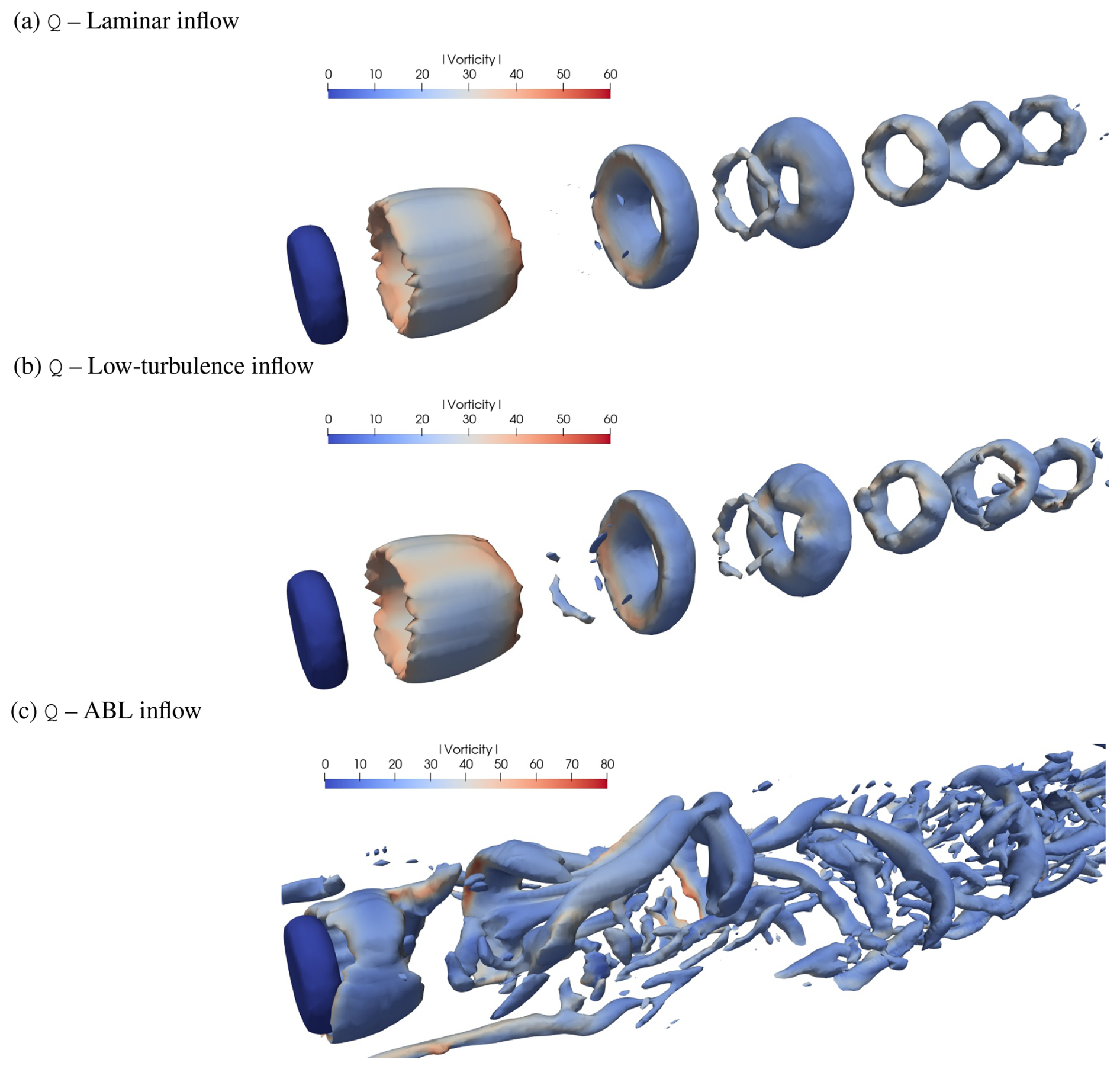
Figure 6 Q criterion contours (Q=50) for S_t=0.32 under laminar (a), low-turbulence (b) and ABL (c) inflows. The contours are coloured by vorticity magnitude.

4 Proper orthogonal decomposition

The POD is a statistical technique originally developed by Lumley (1967) to extract the most energetic coherent structures from turbulent flows by projecting data onto an optimal orthogonal basis. Later, Sirovich (1987) reformulated it into the so-called snapshot method, which made the approach computationally efficient for large datasets. The resulting modes are presented sorted by energy content. The following steps are taken when applying the POD technique in this work. During the last 40 s of each CFD run, once the flow has reached converged statistics, snapshots of the wake are taken in a vertical plane parallel to the AD axis at a sampling frequency of 100 Hz. Data are extracted from 2 D downstream the AD to 10 D, considering only streamwise and vertical velocity components. POD is applied to these results using the MODULO software (Ninni and Mendez, 2020), which implements Sirovich's snapshot method. The result is a decomposition in the form:

$$\begin{array}{}\text{(5)}& u^{\prime }(x,t)=\sum _{P=\mathrm{1}}^N{\mathit{\sigma }}_P{\mathrm{\Phi }}_P\left(x\right){\mathrm{\Psi }}_P\left(t\right),\end{array}$$

where Φ_P and Ψ_P are the spatial and temporal modes respectively sorted by energy content, and σ_P is the square root of the energy of the associated mode. Physically, the spatial modes (Φ_P) represent the most energetic coherent spatial structures of the flow, while the temporal modes (Ψ_P) describe the temporal evolution of the projection of the flow onto each spatial mode. $u^{\prime }(x,t)$ corresponds to the in-plane velocity fluctuations as the mean velocity is subtracted before computing the POD.

In this work, POD spatial modes are used to reveal flow structures that could not be identified using the Q criterion in Sect. 3 and POD temporal modes are used to determine whether the associated flow structures are correlated with the imposed harmonic movement. The latter is done by computing the Fourier transform of the temporal modes. In all cases, the technique is applied to the velocity fluctuations in the plane x−z between 2 D and 10 D downstream the AD. A total of 3600 modes are calculated for each case, and 90 % of accumulated energy is achieved, depending on the frequency, within approximately 10 modes for laminar inflow, 30 modes for low-turbulence inflow and 100 modes for the ABL inflow.

4.1 POD – laminar

The laminar inflow case is considered in the initial stage in order to establish a reference for the subsequent cases. Figure 7 shows the energy content for each mode, which is obtained as the square of the singular value corresponding to the mode in Eq. (5), normalised by the total of this quantity. Results are shown for St=0, St=0.24 and St=0.32, in Fig. 7a, b and c, respectively. These frequencies are representative of all the cases observed (see Table 2). In all figures, the most energetic modes include pairs with similar energy content. Particularly for the cases with surge motion (St=0.24 and St=0.32), this pairing provides a clear baseline to understand how POD captures flow dynamics. In the context of POD, this mode pairing is the mathematical signature of a travelling wave or a convecting coherent structure, such as the vortex rings generated by the AD surge motion. Because these structures continuously change their downstream position over time, a single stationary spatial mode is insufficient to describe them. Consequently, the POD algorithm decomposes this advection into a pair of orthogonal spatial modes that exhibit similar spatial patterns but present a $\mathit{\pi }/\mathrm{2}$ phase shift in the streamwise direction. When these paired spatial modes are multiplied by their corresponding harmonic temporal modes, which oscillate at the same frequency but are also phase-shifted in time, their linear combination accurately reconstructs the continuous downstream advection of the vortices. Following this interpretation, Fig. 8a, b and c show the first four spatial modes for St=0, St=0.24 and St=0.32, respectively. The resulting modes are displayed using vectors indicating the direction of the local velocity fluctuation and are coloured by the fluctuation magnitude, normalised by the maximum value in each case. It is evident that all three cases confirm the presence of pairs of opposite modes (1 and 2, 3 and 4). Also, all modes displayed in pairs present the same Fourier spectrum of the time component (not shown here), thus confirming that they belong to the same vortex structure. The frequencies present in modes 1 and 3 for each case are shown in Fig. 9a, b and c.

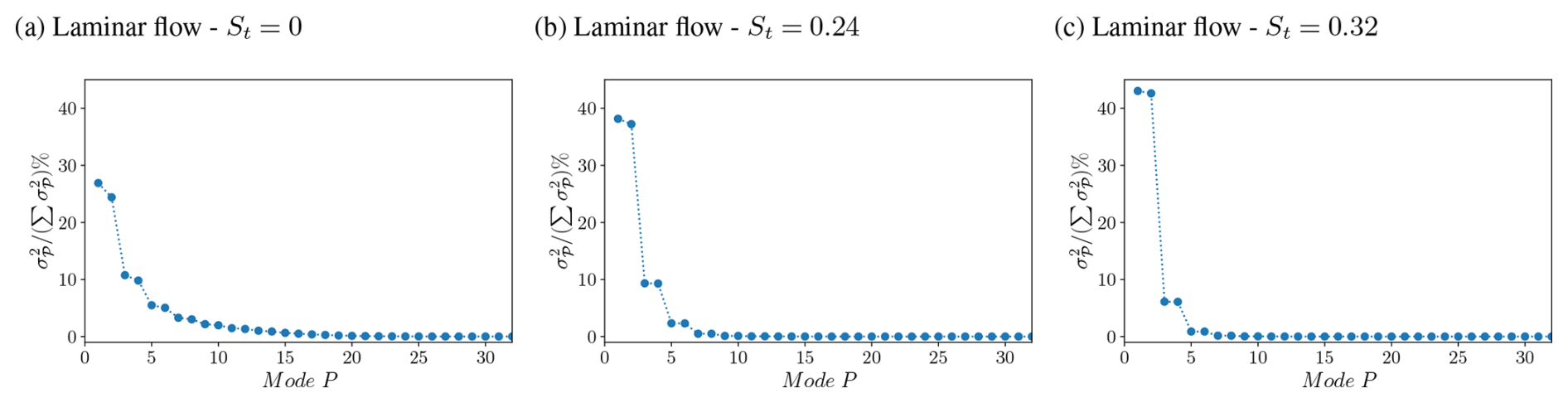
Figure 7 Energy distribution across modes for St=0 (a), St=0.24 (b) and St=0.32 (c), under laminar flow.

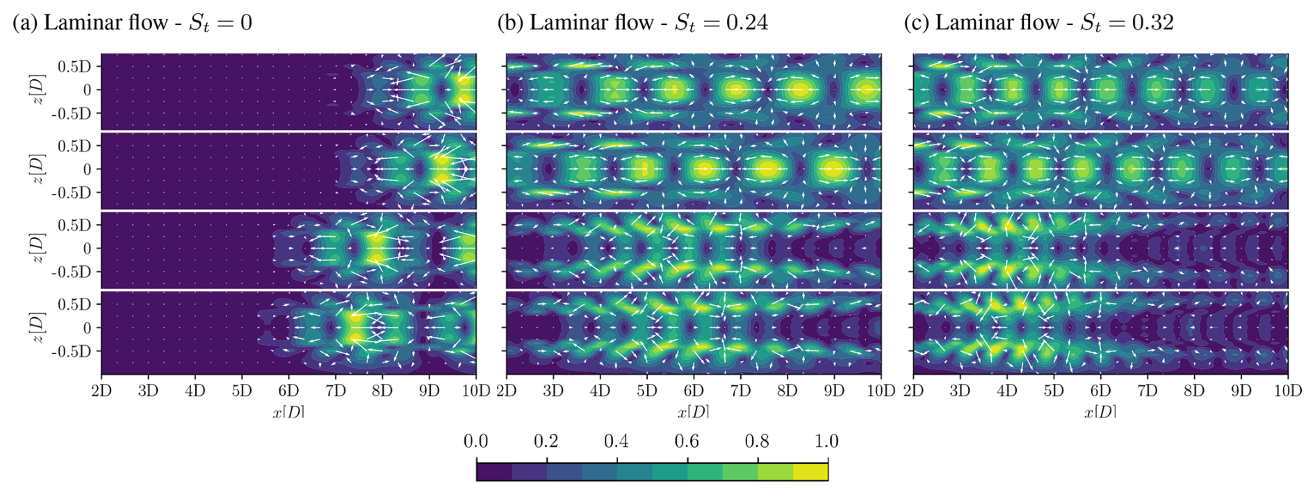
Figure 8 First four spatial modes Φ₁(x)−Φ₄(x) resulting from POD analysis applied to surge cases with St=0 (a), St=0.24 (b) and St=0.32 (c), under laminar flow. The modes are displayed with vectors indicating the direction of the local velocity fluctuation and are coloured by the fluctuation magnitude, normalised by the maximum value in each case.

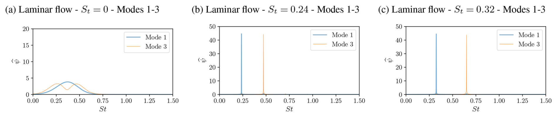
Figure 9 Fourier spectrum of the temporal modes Ψ₁(t) and Ψ₃(t) for St=0 (a), St=0.24 (b) and St=0.32 (c), under laminar flow.

In the absence of motion, that is, when St=0, the spatial modes are found to be symmetric with respect to the AD axis (z=0 in Fig. 8a). This observation indicates that the situation is not one of alternating vortex shedding. Furthermore, the frequencies exhibited in the modes, as illustrated in Fig. 9a, show a distributed energy content across a specific band of frequencies ($\mathit{St}\approx \mathrm{0.2}-\mathrm{0.55}$). While a broadband frequency distribution could theoretically indicate the presence of physical mechanisms whose exact frequency and lateral expansion slowly evolve over time (such as wake meandering), the spatial modes here remain strictly symmetric (Fig. 8a), contradicting an alternating meandering behaviour. Instead, these modes most likely correspond to the advection of negligible residual fluctuations in the wake, as the maximum velocity magnitude reconstructed from them is 6 orders of magnitude smaller than the mean velocity field. This confirms the absence of any dominant coherent structure under stationary laminar conditions.

On the other hand, besides presenting the energy content in pairs (Fig. 7b and c), cases St=0.24 and St=0.32 exhibit a discernible pattern for spatial modes 1 and 2, associated with the advection of the vortex ring structure visualised in Sect. 3 (Fig. 8b and c). In addition, modes 3 and 4 correspond to the first harmonic of this configuration, as illustrated by their spectra in Fig. 9b and c. Also, both pairs of modes present symmetry with respect to the AD axis (z=0) in terms of velocity direction. For modes 1 and 2, the only prevailing frequency is the surge frequency, whereas for modes 3 and 4, it is the double of this frequency. It is noticeable that St=0.32 exhibits higher energy in the first pair of modes and lower energy in the harmonics, compared to St=0.24. In both cases approximately 94 % of the total energy is contained within the first four modes, which is consistent with the findings of Wang et al. (2024), where these modes accounted for about 95 % of the total energy under uniform flow. It is worth mentioning that modes 5 to 10, not shown in this work, behave in a similar way, displaying pairs of different harmonics of the vortex ring structure. Also, in all cases analysed, more than 99.9 % of the energy is accumulated within the first 10 modes, showing that there is no other strong coherent structure present. These observations suggest that the vortex ring structure is a prevailing feature under laminar flow within the specified frequency range. Furthermore, it agrees with the observations made in previous studies, which reported the visualisation of the vortex ring structure for a broad range of frequencies, ranging from St=0.08 to St=1.22, under uniform inflow conditions, as discussed in Sect. 3. In addition, a visual inspection of the spatial modes in Fig. 8 reveals that the coherent pulsation associated with the first pair of modes maintains its structural integrity as it is convected downstream. This persistent coherence is a direct consequence of the complete absence of background turbulence, allowing the structures generated by the surge motion to evolve without external disruption.

4.2 POD – turbulent

The analysis continues with the application of POD to the low-turbulence flow results, with the objective of investigating how the behaviour changes in the presence of turbulence. The energy content for each mode is presented in Fig. 10a, b and c for the cases of St=0, St=0.24 and St=0.32, respectively. These results are followed by the first six spatial modes for each case in Fig. 11a, b and c. In contrast with the laminar no-motion case, where mode pairing was exhibited, the St=0 case presents six distinctly different energy contents for the first six modes characterised by a linear decay (Fig. 10a). Also, the spatial modes in Fig. 11a show asymmetry in terms of velocity direction, as evidenced by the arrows above and below the AD axis (z=0), which point in directions that are not congruent. This suggests an alternating behaviour, such as vertical meandering. Considering the frequency spectrum of modes 1 and 3 (Fig. 12a), it can be seen that the frequency ranges neither match between modes nor show a harmonic relation. The results obtained indicate the presence of meandering phenomena throughout the wake, which is distributed along six modes. A higher energy allocation is observed in the tail of the wake, due to increased wake movement in that sector.

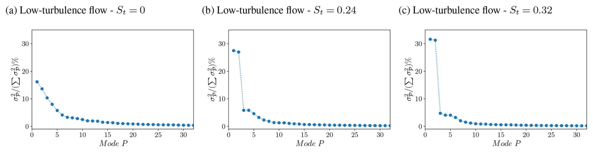
Figure 10 Energy distribution across modes for St=0 (a), St=0.24 (b) and St=0.32 (c), under low-turbulence flow.

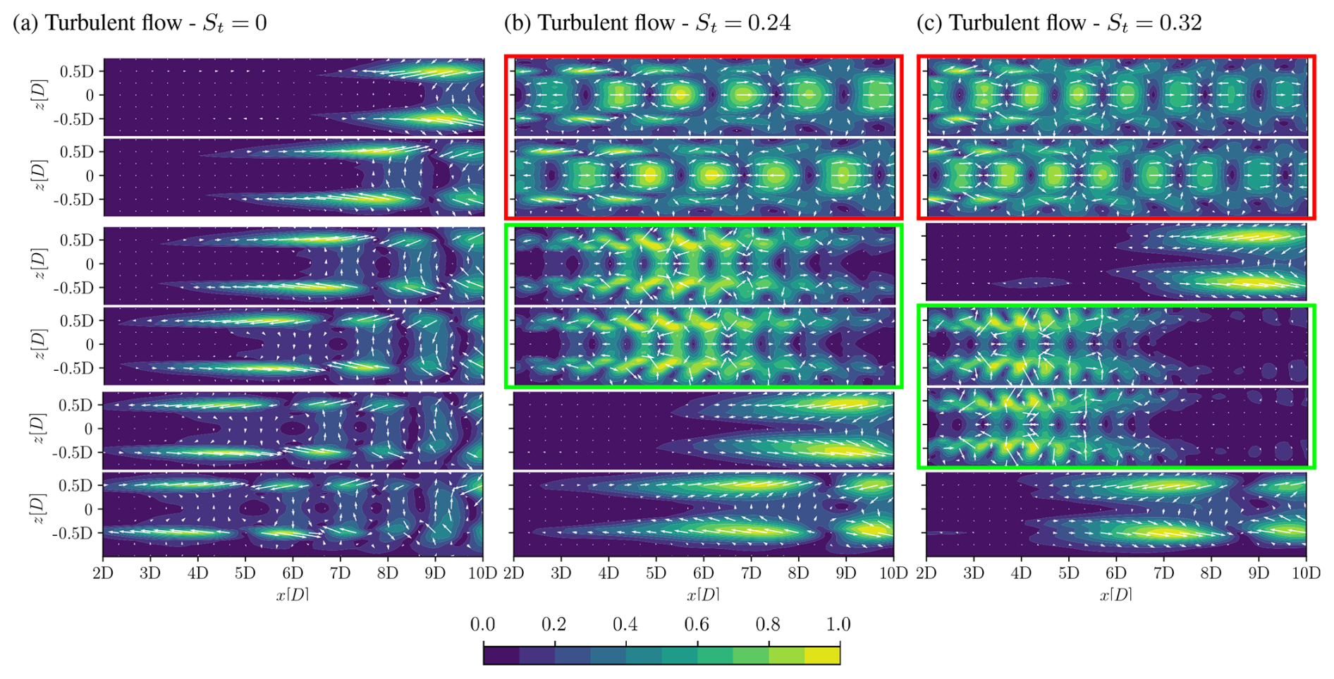
Figure 11 First six spatial modes Φ₁(x)−Φ₆(x) resulting from POD analysis applied to cases with St=0 (a), St=0.24 (b) and St=0.32 (c), under low-turbulence flow. Pairing modes are outlined in red for the case of the main pair (modes 1 and 2 in St=0.24 and St=0.32) and in green for pairing corresponding to harmonics of f_surge (modes 3 and 4 in St=0.24 and modes 4 and 5 in St=0.32). The modes are displayed with vectors indicating the direction of the local velocity fluctuation and are coloured by the fluctuation magnitude, normalised by the maximum value in each case.

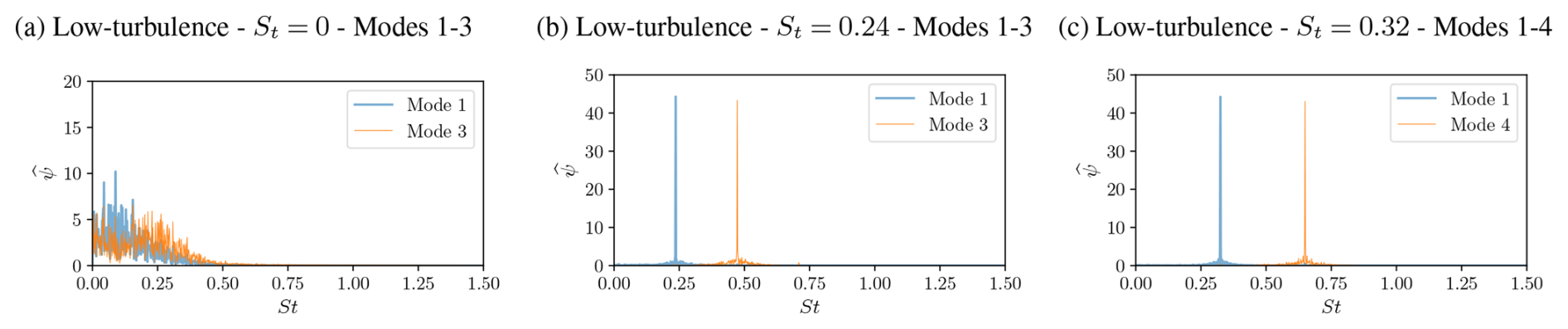
Figure 12 Fourier spectrum of the temporal modes Ψ₁(t) and Ψ₃(t) for St=0 (a), Ψ₁(t) and Ψ₃(t) for St=0.24 (b) and Ψ₁(t) and Ψ₄(t) for St=0.32 (c), under low-turbulence flow.

In the St=0.24 case, it can be observed in Fig. 10b that the first two modes show similar energy content, corresponding to a mode pairing situation. Modes 3 and 4 show a similar pattern. This is confirmed in Fig. 11b, where modes 1 and 2 show pairing corresponding to the vortex ring structure and modes 3 and 4 show a pattern related to the first harmonic of the same structure. These patterns are symmetric with respect to the AD axis (z=0), as it was the case for laminar flow in Fig. 8b. Furthermore, the Fourier spectra of modes 1 and 3 (Fig. 12b) show a single peak corresponding to the surge frequency and twice the surge frequency, respectively. A novel feature is that now, spatial modes 5 and 6 show good agreement with the first two modes in the no motion case. This indicates that, within the most energetic modes, two new modes emerge that are related to the wake meandering rather than the vortex ring structure. The range of frequencies in these modes, not shown here, matches closely with modes 1 and 2 from the St=0 case. Also, the energy distribution presented in Fig. 10b shows that these modes are not paired, resembling the behaviour exhibited for St=0.

For St=0.32, a similar situation is evident for modes 1 and 2, where a clear mode pairing can be seen in Figs. 10c and 11c. This corresponds to the vortex structure shown in Fig. 6b. However, instead of the second harmonic, spatial mode 3 resembles the first mode corresponding to the no-motion case. This means the second harmonic signature is slightly less energetic than for the previous motion frequency, as the corresponding modes fall behind the wake meandering mode. The second mode pairing related to double the surge frequency appears in modes 4 and 5. Finally, mode 6 shows the second mode corresponding to the no-motion case, that is, mode 2 for St=0. In addition, the frequency spectra of modes 1 and 4 displayed in Fig. 12c agree with these observations.

To summarise the results of the POD analysis of the eight cases in Table 2, Fig. 13a and b show the energy content of the first 10 modes for each case. The filled markers connected by a line indicate mode pairing corresponding to the surge frequency, while harmonics are connected with dotted lines. The mode pairing is clear in all cases, where the modes have a similar energy and frequency spectrum. However, the harmonics in St = 0.18 present an arrangement of three modes. In addition, a local maximum is exhibited by the energy content of the pairing modes. This is more clearly seen in Fig. 13c, where the combined energy in both modes and harmonics corresponding to the vortex structure is shown against the St number. The total energy captured by the vortex ring structure for the laminar cases has been added to Fig. 13c for comparison. In the laminar regime, the absence of background turbulence makes the structures generated by the surge motion accumulate nearly 100 % of the kinetic energy across all frequencies. Conversely, under inflow conditions with low turbulence, the energy allocation drops significantly. It is apparent that for the turbulent case at St=0.30, the structure attains its maximum relative energy and subsequently begins a decline as the movement frequency increases. This direct comparison demonstrates that the presence of background turbulence, along with induced phenomena such as wake meandering, severely limits the energy that the vortex rings can retain. Furthermore, contrasting the spatial modes from both regimes (Figs. 8 and 11) reveals that, while the coherent pulsation in the laminar case maintains its amplitude as it convects downstream (first two modes in Fig. 8b), the equivalent structures in the turbulent cases visibly start dissipating in the far wake region. This confirms that even a low level of background turbulence is sufficient to trigger the disruption of the pulsating structures. Ultimately, these results indicate that a characteristic frequency of approximately St=0.30 appears to be the most stable for the propagation of the vortex ring structure under the evaluated conditions with low turbulence.

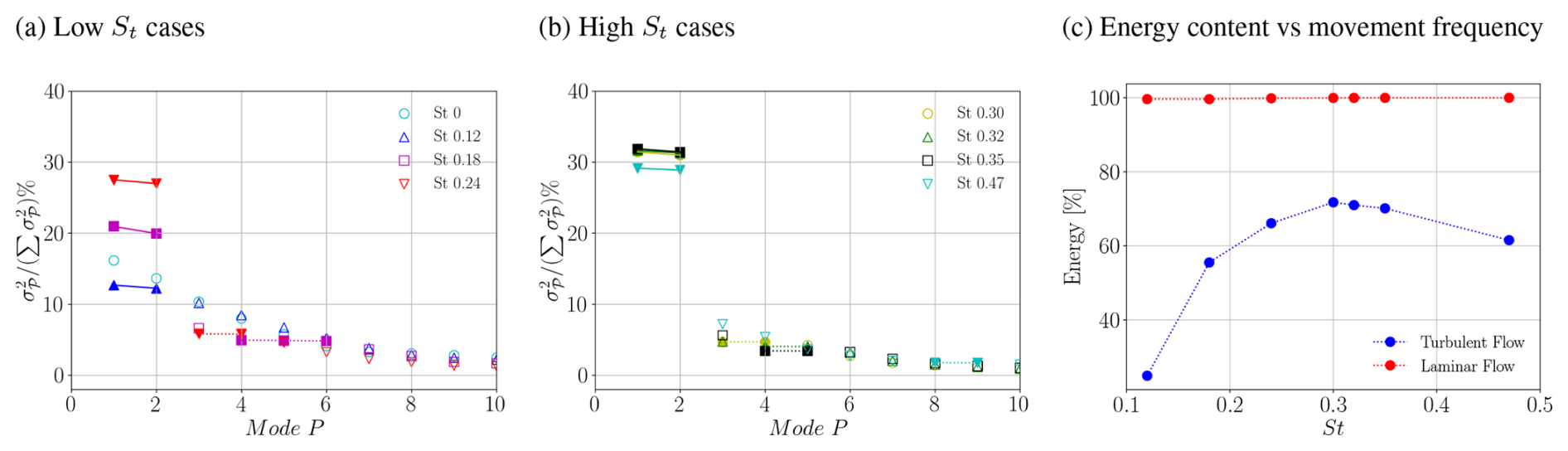
Figure 13 Energy content per mode in low and high St values (a, b) and corresponding to the combined contribution of all modes associated with the vortex ring structure (c) as a function of the St number, under low-turbulence flow. In the first two plots, the filled markers connected by a dashed line indicate mode pairing corresponding to the surge frequency, while harmonics are connected with dotted lines.

4.3 POD – ABL

In the case of ABL flow, the results differ significantly from those of the previous cases. In Fig. 14a, b and c the energy content for each mode is displayed for the cases of St=0, St=0.24 and St=0.32, respectively, followed by the corresponding first six spatial modes in Fig. 15a, b and c. In the no-motion case, the two most energetic modes exhibit an uneven distribution of energy, with the first mode having a markedly higher energy content than the second (Fig. 14a). Also, these two modes exhibit a new spatial distribution (Fig.15a) and a frequency spectrum that spans lower frequencies (Fig. 16a). Instead of a mode pairing situation, the modes can be associated with the inlet ABL flow and its interaction with the AD. Subsequently, modes 3 to 6 manifest distinctive characteristics analogous to those observed in the no-motion case under low-turbulence flow, that is, a quasi-linear behaviour in the energy content decay and a non-symmetric behaviour in terms of velocity direction, as evidenced by the arrows in Fig. 15a. Then, these modes can also be associated with a wake meandering phenomenon divided in four modes, where the energy content is once again higher at the tail of the wake due to a stronger oscillation.

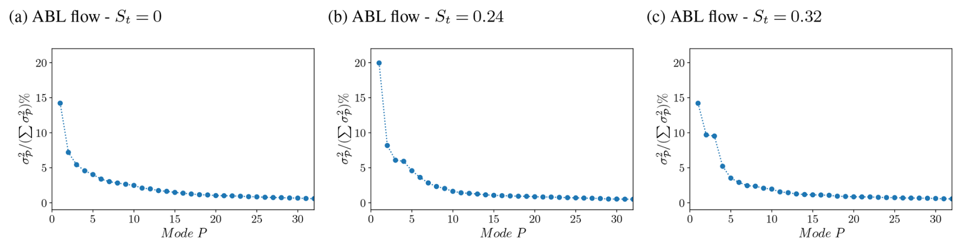
Figure 14 Energy distribution across modes for St=0 (a), St=0.24 (b) and St=0.32 (c), under ABL flow.

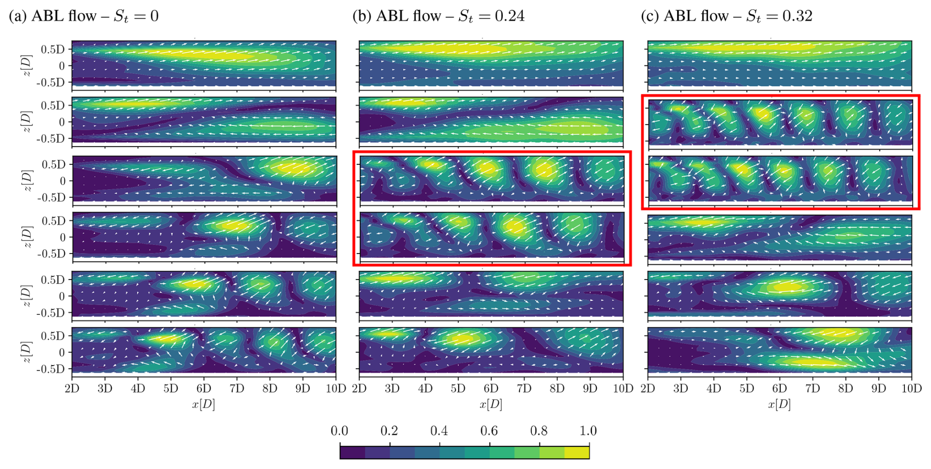
Figure 15 First six spatial modes Φ₁(x)−Φ₆(x) resulting from POD analysis applied to cases with St=0 (a), St=0.24 (b) and St=0.32 (c), under ABL flow. Pairing modes are outlined in red (modes 3 and 4 in St=0.24 and modes 2 and 3 in St=0.32). Modes corresponding to inlet flow and no motion case are the ones resembling modes 1 and 2 in St=0 (modes 1 and 2 in St=0.24 and modes 1 and 4 in St=0.32).

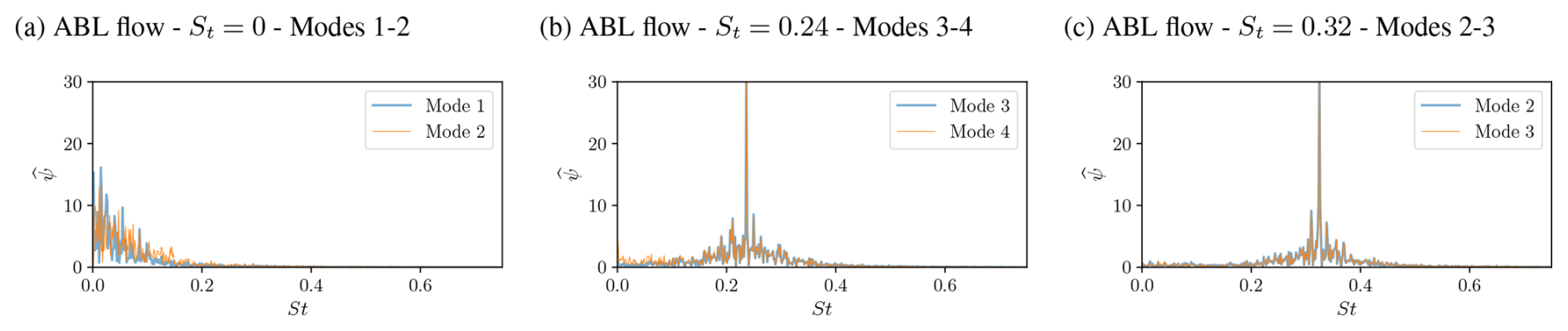
Figure 16 Fourier spectrum of the temporal modes Ψ₁(t) and Ψ₂(t) for St=0 (a), modes Ψ₃(t) and Ψ₄(t) for St=0.24 (b) and modes Ψ₂(t) and Ψ₃(t) for St=0.32 (c), under ABL flow. Modes 1 and 2 for St=0.24 and modes 1 and 4 for St=0.32 have similar spectra as the ones displayed by modes 1 and 2 in St=0.

Regarding the St=0.24 case, Fig. 14b exhibits significantly higher energy in the first mode in comparison to the other modes, as observed in the no-motion case. The vortex pairing can be identified due to the similarity in energy content between modes 3 and 4. Also, it can be noted that the spatial modes 1 and 2 in Fig. 15b show a high degree of agreement with the same modes from St=0. This similarity is absent in modes 3 and 4, where St=0.24 exhibits a pair of opposite modes, as was previously observed in the context of laminar and low-turbulence inflow conditions. Furthermore, the Fourier spectrum of both modes, as illustrated in Fig. 16b, reveals a clear peak at the St that corresponds to the surge movement, with no other frequencies observed. Consequently, it can be deduced that the vortex ring structure is present in this case and that the first two modes are related to the inlet flow and an interaction with the AD similar to that of the no-motion case. Additionally, the Fourier spectrum of these modes, not shown here, exhibit a close match with the ones for modes 1 and 2 in St=0. In this instance, the spatial modes corresponding to the vortex ring structure show no symmetry with respect to the AD axis (z=0) in terms of velocity direction, unlike the laminar and low-turbulence cases. This indicates that, under ABL conditions, the vertical meandering and vortex ring structures are strongly coupled, as the surge motion interacts with the ambient shear flow to induce a synchronised, meandering phenomenon. In relation to the remaining two modes depicted in Fig.15b, mode 5 has not been previously observed and is characterised by an absence of a peak related to the surge frequency in its Fourier spectrum (not shown). Finally a certain degree of similarity is observable between mode 6 and mode 4 from the no-motion case, which can also be related to vertical meandering.

The energy content for St=0.32, displayed in Fig. 14c, shows a single first mode less energetic than for St=0.24, followed by a mode pairing between modes 2 and 3. This indicates that the energy associated with this structure is higher at this frequency than at the previous one, thus explaining the significant reduction in the energy content of the first mode. The energy of the structure was found to vary with the surge frequency for low-turbulence flow, although the vortex pairing shifted to higher modes in this instance. This is corroborated by the spatial modes displayed in Fig.15c, where a first mode similar to the previous cases is shown, followed by a mode pairing between modes 2 and 3. Furthermore, the Fourier spectra depicted in Fig. 16c reveals the absence of any other frequency except that corresponding to the movement. This finding suggests that these modes are exclusively associated with the vortex ring structure. Once again, the modes show no symmetry with respect to the AD axis (z=0) in terms of velocity direction, indicating a vertical meandering phenomenon which is driven by the combination of surge motion and shear flow. Additionally, the spatial mode 4 bears a strong resemblance to mode 2 of the St=0 case, indicating that these modes are not associated with the AD motion but rather with the inlet flow. In a manner analogous to that observed in the St=0.24 case, two novel modes emerge which do not contain the motion frequency in their spectra (5 and 6). Nevertheless, these modes demonstrate the impact of the vortex ring structure on wake behaviour.

Figure 17a and b show the energy share of the first 10 modes for all the cases in Table 2. The filled markers connected by a line indicate mode pairing. Two points merit consideration. On the one hand, the energy associated with modes in the same structure is almost uniform in all cases except for St=0.12 and St=0.18. In the first one, the surge frequency manifested in other modes but no new mode emerged due to the surge motion. In the second, both pairing modes have additional minor peaks of varying frequencies apart from the movement frequency on their spectrum (not shown here), which may have led to alterations in the energy content. This indicates that the convective structures within this range may not yet have attained sufficient strength, consistent with the threshold of St>0.19 reported by Schliffke et al. (2024) for a clear signature at 8 D downstream, under ABL flow. On the other hand, a local maximum is exhibited by the energy content of the pairing modes. This phenomenon is more clearly seen in Fig. 17c, where the combined energy of both modes is shown against the St number. It is apparent that for the case of St=0.32 the structure attains its maximum energy and subsequently begins to decline as the movement frequency increases. Compared with the low-turbulence case in Fig. 13c, a similar pattern is observed in the energy of the structure, which varies with frequency. In this instance, the peak manifests at St=0.32 instead St=0.30 and with a marked increase in the energy content, indicating that a characteristic frequency in proximity to this value favours the propagation of the vortex ring structure for the surge motion conditions studied. Furthermore, the decline in the energy content as the frequency increases is more pronounced in the case of the ABL flow. The presence of more turbulent, complex structures appears to have led to a further reduction in the energy present in the vortex ring structure, given that its energy content is much lower than in the low-turbulence case. In addition, Schliffke et al. (2024) also reported that the highest energy levels occur close to St≈0.30 for ABL, which is in agreement with the values obtained in this work. This comprehensive comparison with laminar and low-turbulence inflows has revealed distinct behaviours of the vortex ring structure and the wake in general within the investigated range when ABL flow is considered.

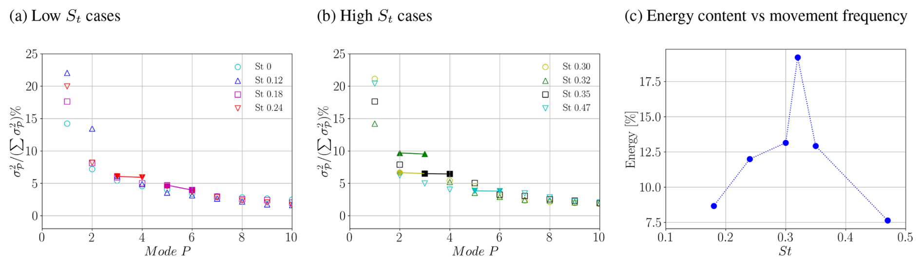
Figure 17 Energy content per mode in low and high St values (a, b) and corresponding to the combined contribution of the two modes associated with the vortex ring structure (c) as a function of the St number, under ABL flow. In the first two plots, the filled markers connected by a dashed line indicate mode pairing.

4.4 Analysis of lateral wake meandering

The POD analysis of a vertical plane revealed, among other details, the presence of vertical meandering for the cases under low-turbulence and ABL inflow conditions. In the low-turbulence scenario, the dynamics of the vortex ring structure and the wake meandering behaved as decoupled phenomena, captured by distinct POD modes with separated frequencies. Furthermore, in neither of the temporal modes did the surge frequency appear within the meandering modes. However, under ABL conditions, these phenomena became highly coupled. The POD mode associated strictly with the surge frequency revealed a spatial structure that inherently includes vertical meandering. This indicates that, in a highly turbulent and sheared environment, the surge motion itself acts as an additional mechanism that triggers induced meandering, phase-locked to the platform's oscillation. In order to delve deeper into this phenomenon, a similar analysis is carried out in this section but on a horizontal plane, with the intention of identifying side-to-side meandering. The data are obtained in the same periods analysed before, with the same sampling frequency. Considering the moving AD at St=0.32, Figs. 18 and 19 show the energy content and spatial modes, respectively, resulting from applying POD analysis to a horizontal plane at hub height under low-turbulence and ABL flow.

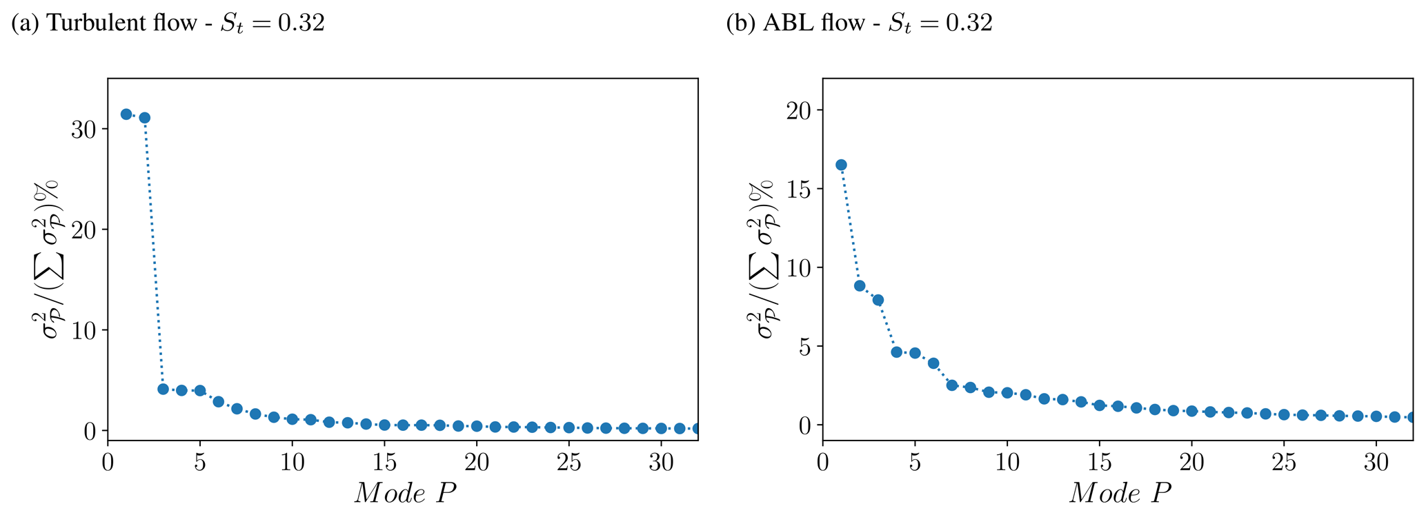
Figure 18 Energy distribution across modes resulting from POD analysis applied to a horizontal plane on cases with St=0.32 under low-turbulence flow (a) and ABL flow (b).

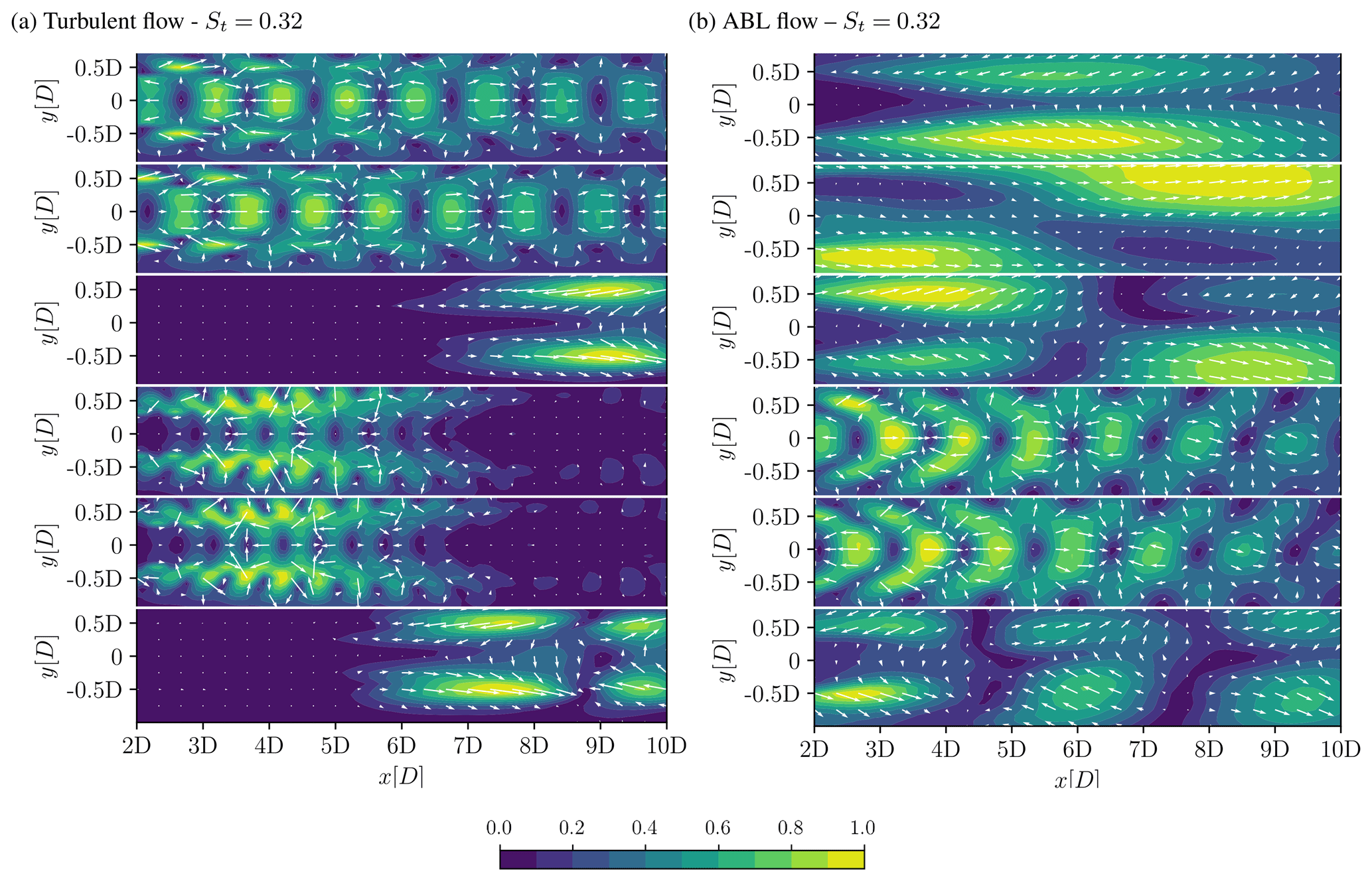
Figure 19 First six spatial modes Φ₁(x)−Φ₆(x) resulting from POD analysis applied to a horizontal plane on cases with St=0.32 under low-turbulence flow (a) and ABL flow (b).

Considering the low-turbulence inflow conditions, Fig. 18a shows an energy distribution across modes that closely resembles that of the vertical plane (displayed in Fig. 10c), with a clear mode pairing situation between modes 1 and 2, followed by three modes with similar energy content. When looking at the spatial modes displayed in Fig. 19a, the results show two mode pairing situations (modes 1–2 and modes 4–5), along with two other modes related to side-to-side meandering (modes 3–6). This is the exact same behaviour as the one presented by the spatial modes on a vertical plane in Fig. 11c. Finally, a similar situation happens when comparing the Fourier spectra of the temporal modes for vertical and horizontal planes (not shown here). These observations allow one to conclude that under low-turbulence inflow conditions, the meandering is present in both vertical and horizontal directions. Given the averaged uniformity of the inflow, it is expected that meandering will occur in the same manner in all directions, as there are no preferred directions.

In contrast, a distinct scenario emerges when considering a horizontal plane for the ABL inflow conditions. Firstly, the energy content of the modes is displayed in Fig. 18b. In this figure, a mode pairing situation can be distinguished between modes 4 and 5, as opposed to modes 2 and 3, as was the case for the vertical plane (Figs. 14c and 15c). In addition, the first mode exhibits a significantly higher energy level in comparison to the subsequent modes, a phenomenon that bears a notable resemblance to the observations presented in Fig. 14c. However, the remaining modes demonstrate a divergent energy content pattern. A detailed analysis of the spatial modes depicted in Fig. 19b reveals significant disparities when compared to the vertical plane modes illustrated in Fig. 15c. The two most energetic modes, which in the previous case were related to the inlet flow, show a different pattern in terms of the spatial modes. Upon analysis of the Fourier spectra in Fig. 20a, it is evident that both modes exhibit a comparable frequency range to the initial two modes observed in the vertical plane case (illustrated in Fig. 16a). This observation suggests that the underlying cause may be the same in both cases. In addition, spatial modes 4 and 5, which are associated with the vortex ring structure, demonstrate a symmetrical pattern with regard to velocity direction until 7 D downstream, as illustrated by the arrows. Beyond this point, the mode begins to manifest signs of asymmetry. This finding suggests that, in a significant proportion of the wake, the vortex ring structure does not exhibit lateral meandering, in contrast to the vertical meandering observed in modes 2 and 3 of Fig. 15c. As demonstrated in Fig. 20b, the Fourier spectra of both modes indicate the absence of any external signal, confirming the presence of a signal exclusively belonging to this structure. In this instance, the modes appear to be more analogous to those observed in the low-turbulence flow case.

Finally, spatial modes 3 and 6 demonstrate a complex pattern that can initially be difficult to identify. At an initial stage, spatial modes 2 and 3 appear analogous; however, a discrepancy in their frequencies prevents a valid basis for the grouping of mode 3 with the inlet flow. A thorough examination of the spatial mode depicted in Fig. 19b reveals that, in the initial phase, the mode undergoes a clockwise rotation during the first half of the wake, followed by an anti-clockwise rotation in the subsequent phase. As is evident in Mode 6, a similar behaviour is exhibited, yet it is divided into three distinct sections. It can thus be theorised that both modes are related to side-to-side meandering. As demonstrated in Fig. 20c, an analysis of the frequency spectra indicates that both modes exhibit a range of frequencies below St=0.2. However, the second mode demonstrates a higher frequency range than the first, due to presenting smaller structures in the spatial mode. Furthermore, in mode 6, a minor peak can be observed at the surge frequency, indicating a minimal presence of surge motion within the mode. However, in contrast to the vertical behaviour, the overall lateral meandering remains physically decoupled from the dynamics of the surge-induced vortex rings.

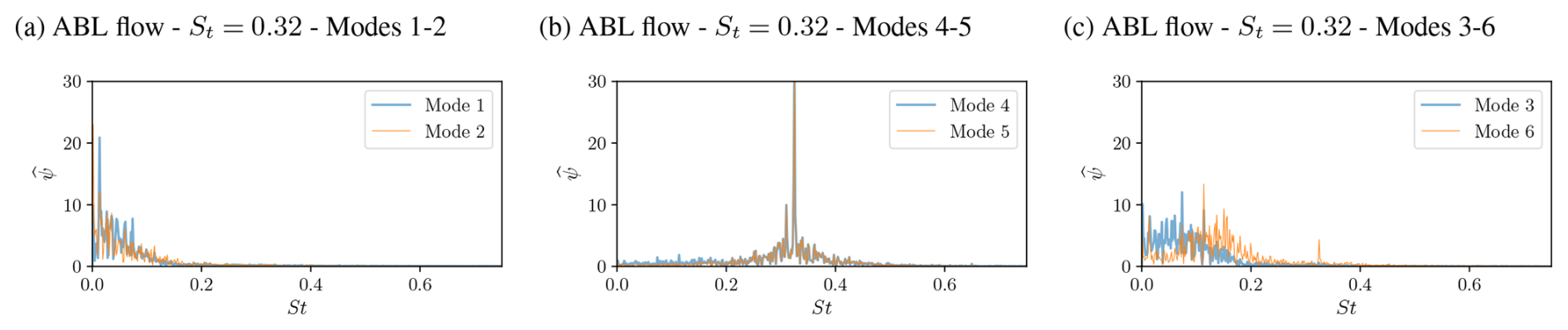
Figure 20 Fourier spectrum of the temporal modes Ψ₁(t) and Ψ₂(t) (a), Ψ₄(t) and Ψ₅(t) (b) and Ψ₃(t) and Ψ₆(t) (c) for St=0.32 under ABL flow.

5 Phase average

The pairing modes visible in Figs. 8, 11 and 15 reveal that the intensity of velocity fluctuations varies depending on the downwind distance, reaching a maximum at a point that depends on each case. The next stage of the analysis focuses on this spatial variation. For this purpose, a phase-averaging procedure is applied to the data planes where the local mean velocity is subtracted in each point. First, the planes of data are re-sampled by linear interpolation to obtain exactly 25 planes within the surge period of each case. Then, every plane is averaged with those sharing the same phase, resulting in 25 planes that contain the averaged fluctuations of one complete surge cycle, $\stackrel{\mathrm{̃}}{u^{\prime }}(x,t)$. Only the fluctuation in the streamwise velocity component was considered in this analysis. Figure 21 shows five planes evenly distributed over the surge period for St=0.32 in the laminar, low-turbulence and ABL flow cases. The results are presented as a percentage of U_ref.

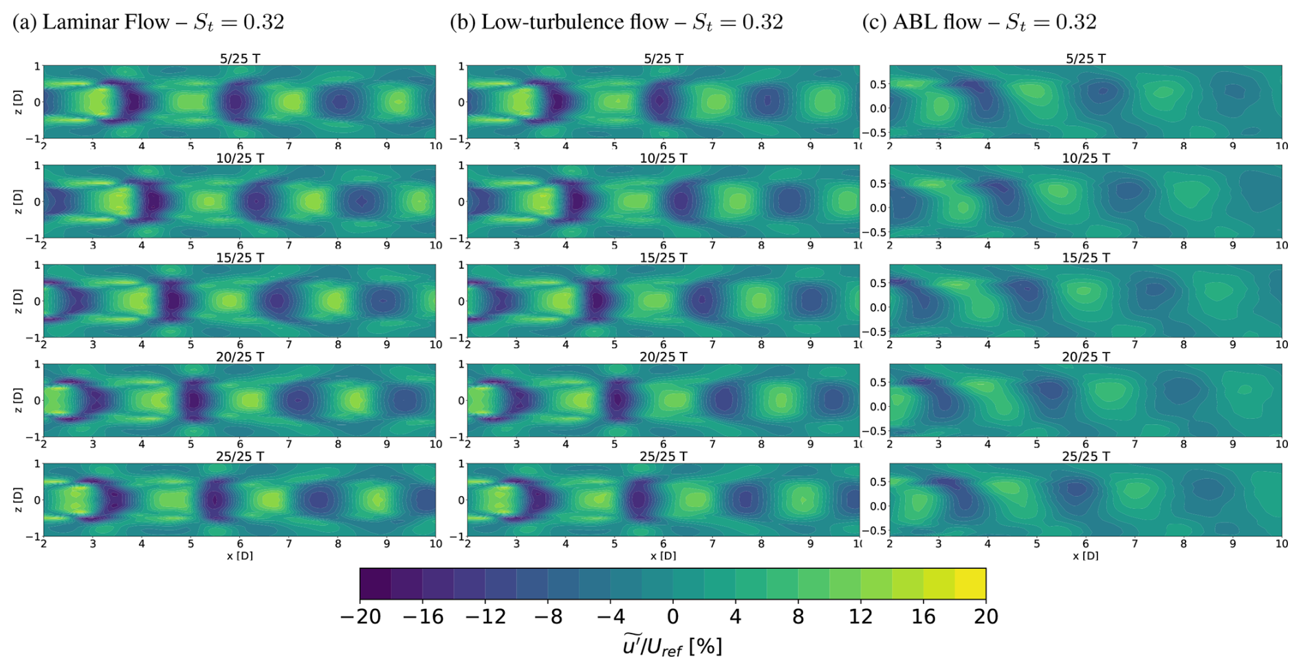
Figure 21 Phase-averaged streamwise velocity fluctuations for laminar flow (a), low-turbulence flow (b) and ABL flow (c). Out of the 25 averaged planes within the surge period, 5 uniformly distributed planes are shown.

The propagation of the structure associated with the surge frequency is visible in all three cases. While the overall configuration remains largely similar, a slight diffusion in the intensity of the velocity oscillations can be observed for the low-turbulence case compared to laminar conditions (Fig. 21a and b respectively). As demonstrated in Sect. 4, the shapes are found to be symmetrical with respect to the AD centreline. It is worth noting that the structural patterns in the phase-averaged fields appear at half the frequency of those in the POD modes since the phase average preserves the velocity sign, whereas the POD representation in Sect. 4 reflects the velocity magnitude. Conversely, for the ABL case (Fig. 21c) the configuration of the structure is modified by the ABL's shear flow. Moreover, the ABL case presents the maximal velocity variations at approximately one-quarter of the diameter above the centre of the disc. In contrast, in the other cases, these values appear at the centre of the disc. This result aligns closely with the findings reported in Schliffke et al. (2024), where the highest signature values were observed in the wake at points situated along a vertical line positioned above the disc centre. Regarding the structural patterns, in both the laminar and low-turbulence cases, the regions of minimum fluctuation along the AD centreline appear to merge with off-centre zones, forming an upstream-facing curvature (towards the left) in the near wake (x< 5 D). Further downstream, this pattern seems to invert into downstream-facing arcs. This behaviour could be attributed to the difference in advection velocities inside and outside the wake, a hypothesis that will be thoroughly analysed in the subsequent subsection. In the ABL scenario, the lower-fluctuation structures initially exhibit a downstream tilt up to x≈ 4 D, likely resulting from the reduced advection velocity below the centreline caused by the shear flow. Beyond this point, an apparent sudden shift in inclination occurs, which may be caused by the merging of a low-velocity region from one structure with the subsequent one. Given the complexity of these flow features, they will be examined in greater detail and with clearer visualisations in the following subsection.

Sampling along a line at the vertical position where the maximum oscillation occurs (the centre (z=0) for laminar and low-turbulence flows and $z=\frac{\mathrm{1}}{\mathrm{4}}$D for ABL) and recording half the amplitude between the maximum and minimum values reveals the spatial propagation dynamics of the pulsating mode, as shown in Fig. 22. The majority of cases demonstrate an initial increase, subsequently followed by a decline in amplitude throughout the wake. In the laminar case (Fig. 22a), as the frequency increases, the amplitude peak is presented closer to the AD and the decay begins sooner in the wake. In particular, the case of St=0.47 shows the fastest decay. Also, lower frequencies exhibit higher amplitude peaks, with the exception of St=0.12. It is possible that a higher peak may be present further in the wake for this case, although this point is not attained in the present study. Considering a reference distance of 8 D from the AD, which was described as an optimum balance for large offshore wind farms by Sørensen et al. (2021), it can be observed that, with the exception of the highest frequency, all cases present a fluctuation of over 10 % and even over 15 % of the inlet velocity.

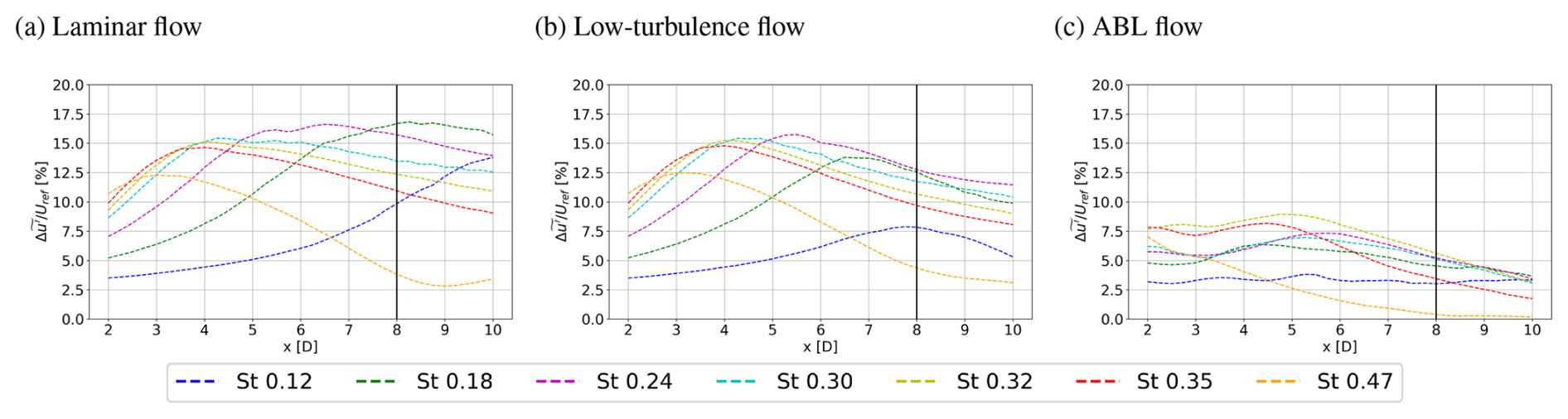
Figure 22 Half amplitude between the maximum and minimum value for the phase-averaged velocity fluctuation within one period. Laminar and low-turbulence values are extracted at the AD centre, while ABL values are extracted at $\frac{D}{\mathrm{4}}$ above the AD centre.

In the case of low-turbulence flow (Fig. 22b), all cases show a faster decay of the signal towards the end, with the exception of the highest frequency, which shows a similar behaviour than in the laminar case, with the peak value at 3 D and a continuous decay until 9 D. In particular, compared with the laminar inflow, the most-affected cases seem to be the lower frequencies, St=0.12–0.24, as their shift towards the AD, producing an earlier onset of decay compared to previous observations. As demonstrated in Sect. 4, the aforementioned cases exhibited the lowest energy levels in the vortex ring structure. Contrary to this, the cases with higher energy content in Sect. 4, St=0.30–0.35 exhibit a peak close to 4 D, both with and without turbulence. This may indicate that for those frequencies that favour the energy content of the vortex ring structure, the growth rate and spatial propagation up to the peak value is unaffected by turbulence. Finally, for the highest frequency, St=0.47, the spatial behaviour remains almost unaltered, although the decay was already rapid under laminar flow. It is notable that all cases maintain an amplitude almost over 10 % at 8 D from the AD, with the exception of the highest and lowest frequencies.

Finally, in the ABL flow case (Fig. 22c), it is evident that all cases display a more pronounced decay towards the end than in previous inflow conditions. Nonetheless, the case St=0.32, which demonstrated the higher energy content in Sect. 4, exhibits a higher amplitude throughout the entire wake. In addition, the case with St=0.12 that previously exhibited no mode pairing related to the vortex ring structure maintains a low amplitude for the entire wake, demonstrating an absence of ascending–descending behaviour. Once again, St=0.47 exhibits accelerated decay. It can be pointed out then that, similar to the low-turbulence case, the spatio-temporal behaviour of the structure deviates from the ideal laminar inflow conditions, and the extent of deviation is contingent on the energy content of the vortex structure for a given surge frequency. This specific behaviour is not observed in the highest frequency case, wherein the decay always exhibits a faster rate. Compared with the inlet velocity, three of the analysed cases remain with an amplitude over 5 % at 8 D, while the remaining cases exhibit a decay that falls below this threshold.

A thorough examination of the three plots in Fig. 22 reveals that the strongest surge motion signature in the wake at 8 D occurs at St=0.18 for laminar flow, St=0.24 for low-turbulence flow and St=0.32 for ABL flow. However, it is important to note that this observation should not be confused with the energy content discussed previously in Sect. 4, as the present analysis focuses on the response at a specific height, whereas the earlier analysis considered the vortex structure at all heights.

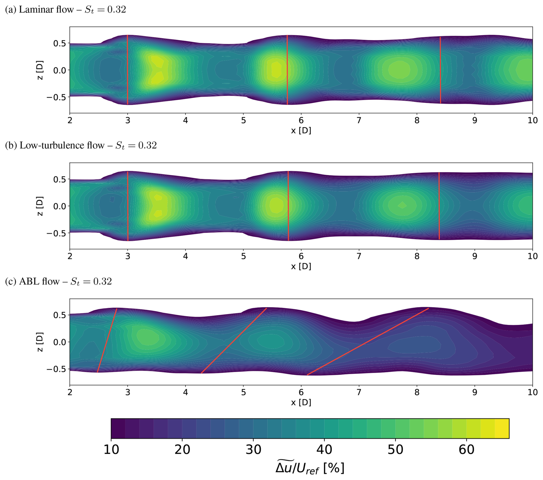
Figure 23 Phase-averaged streamwise velocity deficit for laminar flow (a), low-turbulence flow (b) and ABL flow (c). For each case, only 1 out of the 25 averaged planes is shown. Red lines connect the expansion tops and bottoms for the first three cycles in each case.

5.1 Spatio-temporal wake modulation

As demonstrated in Sect. 4, while the surge motion generates decoupled vortex ring structures under uniform inflows, the ABL shear flow couples with these structures to induce a synchronised vertical meandering. Furthermore, distinct spatial patterns emerge depending on the inflow, ranging from symmetric wake modulation to a noticeable structural inclination of the velocity fluctuations in the ABL scenario (as illustrated in Fig. 21c). In this section, a more profound examination of these varied wake configurations is proposed. To this end, the velocity deficit will be subjected to phase averaging in place of velocity fluctuations. This approach is intended to provide a more precise depiction of the wake's configuration during surge motion. The process is analogous to the previous analysis but rather than subtracting the mean flow values, the inflow profiles displayed in Figs. 4a and 5a are subtracted considering the corresponding case. Once again, 25 planes are obtained, containing in this instance the velocity deficit, $\stackrel{\mathrm{̃}}{\mathrm{\Delta }u}(x,t)$. In this analysis, the focus was exclusively on the streamwise velocity component. Figure 23 illustrates one of the frames for St=0.32 in the laminar, low-turbulence and ABL flow cases. The results are presented as the percentage of U_ref.

In the laminar and low-turbulence cases, illustrated in Fig. 23a and b, the averaged velocity deficit exhibits a wake modulated by an expansion and contraction due to the surge motion. This behaviour aligns closely with the synchronised coherent pulsing experimentally observed by Messmer et al. (2024) under laminar inflow at a comparable Strouhal number (St=0.38 vs. St=0.32). Furthermore, recent ABL wind tunnel tests by Hubert et al. (2025) confirmed that these periodic wake expansions persist even at a lower frequency (St=0.11), while numerical evaluations attribute this overall dynamic to strong variations in the rotor's axial induction (Sivalingam et al., 2018). As demonstrated in the case of fluctuations in Fig. 21, there is a minimal difference between laminar and low-turbulence inflow with regard to this aspect. The only discernible discrepancy manifests towards the culmination of the wake, in proximity to 10 D, where the contraction is more pronounced in the laminar inflow scenario. Conversely, in the context of ABL flow, as illustrated in Fig. 23c, the phase average deficit reveals a wake characterised by traces of contraction and expansion, coupled with a vertical deformation induced by the background wind shear. Red lines in the three panels connect the expansion tops and bottoms for the first three cycles in each case. For the first two scenarios, the lines maintain a parallel configuration throughout the wake. It is evident that, in the initial line on the left, the maximum deficit is situated to the right of the red line. For the second and third lines, the maximum deficit is observed to the left of the line. This phenomenon is attributable to a disparity in advection velocity, whereby maximum deficit structures travel slower within the wake in comparison to the expansion and contraction observed at the periphery of the wake. The lines in the ABL case, in contrast to the first two cases, show an inclination towards the right. Furthermore, it has an increasing tendency further away from the AD original position. This phenomenon is attributable to the effects of shear flow, which modify the translation velocity of the vortex structure above and below the AD centreline. As was evidenced in the preceding cases, the expansion regions situated above the wake appear to travel faster than the maximum deficit structures. However, it is now evident that the expansion regions situated below the wake travel slower. Consequently, this disparity in translation velocities causes the surge motion to couple with the shear flow, inducing a synchronised vertical meandering. This phenomenon was also observed by Hubert et al. (2026), who conducted a SPIV analysis at 8.125 D from the position of a porous disc under surge motion. In addition, the configuration of the maximum deficit structures appears to undergo a transformation throughout the wake, as evidenced by the iso-deficit lines. Furthermore, an increase in velocity above the AD centreline results in a greater force acting on the top than on the bottom, leading to greater fluctuations over the AD axis.

6 Conclusions

In this work, new physical insights were achieved regarding the vortex ring structure that appears downstream a FOWT model under surge motion, by comparing its dynamics under realistic ABL conditions against laminar and low-turbulence flows. For the ABL inflow configuration, the numerical results were also analysed in relation to the reference wind tunnel experiments, showing generally consistent trends in terms of the dominant physical mechanisms, dynamic thresholds and spatial energy distribution. The structure was first visualised by means of the Q criterion for laminar and low-turbulence uniform inflows, while no discernible pattern was observed under ABL inflow, in line with previous works. Subsequently, a POD analysis was conducted for the three inflow conditions. In the laminar flow configuration, the method allocated more than 99 % of the energy to the vortex ring structure generated by the harmonic surge motion applied to the actuator disc, displaying pairs of opposite modes associated with the surge frequency and multiple harmonics. In this instance, all modes displayed symmetry with respect to the AD centreline, indicating no meandering phenomenon. Additionally, the low-turbulence case also displayed pairs of opposite modes related to the vortex ring structure which were symmetric in terms of velocity direction. Yet, these were combined with non-symmetric modes related to the no-motion case, which were linked to the wake meandering phenomenon. The energy content analysis confirmed that the signature related to the vortex ring structure shows a local maximum in the studied frequency range.

In the context of the ABL inflow scenario, a divergent tendency was identified, manifesting a single pair of opposite modes associated with the surge frequency and two high-energy modes linked to the inlet flow. The latter were observed in both motion and no-motion cases. In this instance, no harmonic of the surge frequency was excited within the most energetic modes. Furthermore, in cases involving a moving AD, the modes related to the vortex ring structure exhibited asymmetry with respect to the AD centreline, thereby indicating the presence of meandering in such modes. In the absence of any other significant peaks in the Fourier spectra, it can be concluded that under ABL conditions, the combination of surge kinematics and background shear induces synchronised vertical meandering. A more thorough investigation into the meandering phenomenon revealed that, while meandering occurs in every direction with equal intensity for the low-turbulence inflow case, under ABL conditions the lateral and vertical meandering are produced by different factors. While the vertical meandering is strongly linked to the surge motion, the lateral meandering remains physically decoupled from the vortex ring dynamics and is driven by different atmospheric factors. In both low-turbulence and ABL inflows, the highest energy content structures manifested at St values consistent with those observed in previous experiments. However, distinct behaviours were observed, with the ABL case exhibiting a narrower energy distribution. It was determined that the no-motion modes were more significant under ABL than under low-turbulence inflow. Consequently, the generation of structures related to the vortex ring structure with higher energy was observed in the latter.

The phase-averaging analysis of velocity fluctuations yielded further insights into the spatio-temporal dynamics, propagation and growth rates of the structure and how these are affected by inlet conditions. In laminar and low-turbulence cases the structure demonstrated a symmetrical configuration. However, in the ABL case, the shear flow modified the modes, thereby shifting the location of fluctuation extrema, which is consistent with previous experimental observations. Furthermore, both low-turbulence and ABL flow showed a diminished impact on growth rate for those frequencies that developed the most energetic structures. In both cases, the decay towards the end was faster than under laminar inflow. Finally, the majority of cases exhibited an amplitude in over 10 % of the inlet velocity at 8 D downstream the AD, under low-turbulence flow, which aligns closely with the findings observed in laminar inflow conditions. In contrast, for the ABL case, this value declined to approximately 5 % or less, depending on the specific case scenario.

Finally, to obtain a thorough analysis of the shape of the wake, phase averaging was applied to the velocity deficit. The present study has demonstrated that, in laminar and low-turbulence cases, the wake is modulated by an expansion and contraction in response to surge motion. This periodic behaviour firmly corroborates the phase-locked coherent pulsing documented in recent wind tunnel experiments at comparable Strouhal numbers. Conversely, under ABL flow, the study revealed traces of this modulation coupled with a vertical deformation induced by the background wind shear. This phenomenon was attributed to the disparity in translation velocity between the lower and upper regions of the structure. This phenomenon was also visualised in recent wind tunnel experiments under ABL conditions.

Despite the robustness of the AD model in capturing the far-wake evolution, this approach inherently bypasses the initial generation of discrete helical tip vortices and their subsequent breakdown into vortex ring structures. Consequently, future work should extend this analysis using ALM or blade-resolved simulations to capture these near-wake dynamics and investigate how these helical tip vortices behave and transition under realistic ABL conditions. Overall, this study establishes that while the surge-induced wake modulation and its energy–frequency dependence persist across different inflows, the highly turbulent and sheared nature of the ABL introduces unique dynamics. Specifically, the combined effects of atmospheric shear and elevated background turbulence not only structurally deform the wake but also induce a directional decoupling of the meandering phenomenon. These findings emphasise the need for further research under realistic atmospheric conditions, where marine atmospheric boundary layer thermal stability should be taken into account in the analysis of FOWT wakes.