Large-eddy simulation of thermally stratified atmospheric boundary layers with a lattice Boltzmann method

Thermal stratification plays an important role in wind farm flows and must therefore be included in simulations of such flows. At the same time, wind farms are covering larger areas, requiring very large domains and leading to exceptional computational costs for large-eddy simulations (LESs). The lattice Boltzmann method (LBM) is a novel approach to LES of wind farm flows that is particularly efficient and suitable for massively parallel hardware, such as graphics processing units (GPUs). In this work, we present a novel model for LES-LBM of stratified atmospheric boundary layers, using a so-called double-distribution function approach. We develop a novel boundary condition to apply Monin–Obukhov similarity theory and implement a number of other components required for simulations of stratified boundary layers in the GPU-resident version of the open-source LBM solver VirtualFluids. The model is validated for conventionally neutral and stably stratified boundary layers. Results agree closely with numerical references. The model is able to simulate conventionally neutral boundary layers with parameters typical for wind energy applications of the order of real time on a single GPU. Future work will include development of a precursor–successor method for wind farm flow simulations and improvements to the collision operator of the temperature model.

1 Introduction

Wake recovery (Abkar and Porté-Agel, 2015), the persistence of wind farm wakes (Platis et al., 2022), and the occurrence of gravity waves (Lanzilao and Meyers, 2024) all depend on the thermal stratification of the atmospheric boundary layer (ABL). Large-eddy simulation (LES) enables the most accurate examination of these phenomena that is feasible with currently available hardware. Wind farms or clusters of wind farms cover large areas, yet simulations need to be well resolved to fully capture the behavior of the boundary and inversion layer (Allaerts and Meyers, 2017). The resulting simulations thus feature extremely large numbers of degrees of freedom. Current LES models for the ABL, typically CPU-resident finite-volume or pseudospectral solvers, require days or months of computing time on very large compute clusters to perform such simulations.

A new generation of solvers seeks to alleviate the immense computational cost by utilizing graphics processing units (GPUs), such as MircoHH (van Heerwaarden et al., 2017), AMR-Wind (Kuhn et al., 2025b), and FastEddy (Sauer and Muñoz-Esparza, 2020). van Heerwaarden et al. (2017) report that 32 CPU cores are necessary to achieve the same computational performance as one NVIDIA Quadro K6000. Sauer and Muñoz-Esparza (2020) have already reported that 1 GPU equals the performance of 256 CPU cores, highlighting the rapidly increasing speed of GPUs.

However, a different approach, based on the lattice Boltzmann method (LBM), has also been introduced to wind energy and boundary layer research over the last decade. A recent review can be found in Korb et al. (2026). The LBM's mathematical structure is well suited for the use of massively parallel hardware, such as GPUs. In the LBM, fluid is described as a set of populations on the nodes of a Cartesian grid. The LBM then follows a two-step algorithm. First, the populations at a node collide, then they are advected to neighboring nodes (Krüger et al., 2017). The collision step is potentially non-linear but is a local operation, while the advection step simply consists of moving memory on a computer. While initial formulations of the LBM were unstable at high Reynolds numbers, recent advances in the formulation of the collision step have rendered it a suitable method for high-Reynolds flows and LES (Geier et al., 2015, 2020; Jacob et al., 2018).

LES based on the LBM has been used now for over a decade to simulate large-scale boundary layer flows. Onodera et al. (2013) present a simulation of 10 km × 10 km of Tokyo's urban area at a 1 m resolution on up to 1000 GPUs, demonstrating the method's suitability for very large problems. Further examples of simulations utilizing GPUs include King et al. (2017) and Lenz et al. (2019). Both report near-real-time computational performance, demonstrating the high computational efficiency of the LBM on GPUs. None of the aforementioned simulations include wall models. Asmuth et al. (2021) introduced a wall-modeling approach suitable for atmospheric boundary layers and showed very good agreement with reference results.

All of the aforementioned models only consider isothermal boundary layers, and very few models considering thermal stratification have previously been presented in the literature. The temperature equation can be discretized either via “traditional” approaches, such as finite difference or finite volume, or via a modified LBM. The former is named a hybrid approach, while the latter is referred to as a double-distribution function approach (DDF). A hybrid approach was applied in one of the earliest studies of stratified boundary layer flows with the LBM, the TheLMA project, described in a series of publications (Obrecht et al., 2012, 2013, 2015). Another solver designed for atmospheric boundary layers implementing a hybrid approach is presented in Feng et al. (2021). ProLB employs the hybrid recursive regularized collision model (Jacob et al., 2018) and the wall-modeling approach by Malaspinas and Sagaut (2014). However, it is not mentioned that it utilizes GPUs, and no remarks on its computational performance are given. An overview of advection–diffusion LBM models can be found in Gruszczyński and Łaniewski-Wołłk (2022), where the authors also compare a number of more advanced LBM models. They find that models based on the cascaded LBM yield the most accurate results. A similar model is applied in Alihussein et al. (2021) to simulate the dissolution in porous media. Wang et al. (2020) present a method using the DDF approach for simulation of the stratified flow over a ridge. Both LBM models (for momentum and temperature) employ a multiple-relaxation time method (d'Humières, 1994).

In this paper, we propose a novel model to simulate the stratified atmospheric boundary layer via a DDF LBM model based on the cumulant LBM for momentum and a factorized cascaded model for the advection–diffusion equation. We describe the methodology in Sect. 2. We compare results obtained with our method to reference data for both a neutral and a stably stratified test case in Sect. 3 and give our concluding remarks in Sect. 4. As with any model development, we tried many different variants until we converged on the model we present here. We document some of those approaches in Appendix A.

2 Methodology

We will be begin by describing the fundamentals of the cumulant lattice Boltzmann method and its modifications to simulate atmospheric boundary layers. Subsequently, we present the method used to simulate the advection–diffusion of the potential temperature. Finally, we discuss novel formulations for boundary conditions and other aspects specific to modeling thermally stratified boundary layers.

2.1 Governing equations

Our aim is to simulate the filtered incompressible Navier–Stokes equations with Coriolis forces coupled to an advection–diffusion equation of potential temperature via the Boussinesq approximation (see Stoll et al., 2020, and references therein):

$$\begin{array}{}\text{(1)}& {\displaystyle }& {\displaystyle \frac{\partial u_i}{\partial x_i}}=\mathrm{0},\text{(2)}& {\displaystyle }& {\displaystyle \frac{\partial u_i}{\partial t}}+u_j{\displaystyle \frac{\partial u_i}{\partial x_j}}=-{\displaystyle \frac{\mathrm{1}}{{\mathit{\rho }}_{\mathrm{0}}}}{\displaystyle \frac{\partial p}{\partial x_i}}+{\displaystyle \frac{\partial }{\partial x_j}}\left({\mathit{\nu }}_{\mathrm{e}}{\displaystyle \frac{\partial u_i}{\partial x_j}}\right)+F_i^{\mathrm{C}}+F_i^{\mathrm{B}},\text{(3)}& {\displaystyle }& {\displaystyle \frac{\partial \mathit{\theta }}{\partial t}}+u_j{\displaystyle \frac{\partial \mathit{\theta }}{\partial x_j}}={\displaystyle \frac{\partial }{\partial x_j}}\left(D_{\mathrm{e}}{\displaystyle \frac{\partial \mathit{\theta }}{\partial x_j}}\right).\end{array}$$

Here, the coordinate system is denoted as $\mathit{x}=[x,y,z{]}^{\mathrm{T}}$; t is time; ρ₀ is the density; u is the filtered velocity; p is the pressure deviation from the background pressure; θ is the filtered potential temperature; the Coriolis and buoyancy forces are F^C and F^B, respectively; and subgrid stresses and heat flux are parameterized via an effective viscosity and diffusivity, ν_e and D_e, respectively. We use Einstein's summation convention. The Coriolis force is given by

$$\begin{array}{}\text{(4)}& F_i^{\mathrm{C}}=-{\mathit{ϵ}}_{ij\mathrm{3}}(G_j-u_j)f_{\mathrm{c}},\end{array}$$

where ϵ_ijk is the Levi–Civita symbol, $\mathit{G}=G[\cos \mathit{\alpha },\sin \mathit{\alpha },\mathrm{0}{]}^{\mathrm{T}}$ is the geostrophic wind with the geostrophic wind speed G and direction α, and f_c=2Ωsin φ is the Coriolis parameter that depends on the rotational speed of the Earth Ω and latitude φ. The Boussinesq approximation assumes $F_i^{\mathrm{b}}=g\frac{\mathit{\theta }-{\mathit{\theta }}_r}{{\mathit{\theta }}_r}{\mathit{\delta }}_{i\mathrm{3}}$, where g is the gravitational acceleration, θ_r is a reference temperature, and δ_ij is the Kronecker delta. However, to remove the hydrostatic pressure, we take the horizontal average, denoted by 〈⋅〉, of Eq. (2) with i=3, following, e.g., Deardorff (1970). We find that $\frac{\mathrm{1}}{{\mathit{\rho }}_{\mathrm{0}}}\frac{\partial \langle p\rangle }{\partial z}=\frac{\langle \mathit{\theta }\rangle -{\mathit{\theta }}_{\mathrm{0}}}{{\mathit{\theta }}_{\mathrm{0}}}$, since the continuity equation dictates 〈u₃〉=0. Splitting p into $p^{\prime }+\langle p\rangle$ and inserting the previous result in Eq. (2), we can write

$$\begin{array}{}\text{(5)}& F_i^{\mathrm{B}}=g{\displaystyle \frac{\mathit{\theta }-\langle \mathit{\theta }\rangle \left(z\right)}{{\mathit{\theta }}_{\mathrm{r}}}}{\mathit{\delta }}_{i\mathrm{3}}\end{array}$$

if we replace p by p^′. Contrary to “classical” computational fluid dynamics, we do not discretize these equations but instead solve them via the lattice Boltzmann method implemented in the GPU-resident version of the open-source solver VirtualFluids (Geier et al., 2025).

2.2 The cumulant lattice Boltzmann method

The fundamental variable of the lattice Boltzmann method is the particle distribution function (PDF) f. The PDF describes the probability of encountering a particle with velocity ξ at time t and location x. The discretization of velocity space to a lattice of discrete velocities ${\mathit{c}}_{\mathit{\iota }\mathit{\kappa }\mathit{\lambda }}=(\mathit{\iota }{\mathit{\delta }}_{i\mathrm{1}}+\mathit{\kappa }{\mathit{\delta }}_{i\mathrm{2}}+\mathit{\lambda }{\mathit{\delta }}_{i\mathrm{3}})c$, with $c=\frac{\mathrm{\Delta }x}{\mathrm{\Delta }t}$ as lattice velocity, leads to the discrete populations $f_{\mathit{\iota }\mathit{\kappa }\mathit{\lambda }}(\mathit{x},t):=f({\mathit{c}}_{\mathit{\iota }\mathit{\kappa }\mathit{\lambda }},\mathit{x},t)$. Following Geier et al. (2015), we denote lattice directions with triplets of Greek indices corresponding to their directions in space and define $\stackrel{\mathrm{‾}}{\mathit{\iota }}:=-\mathit{\iota }$. Note that Greek indices are not subject to the summation convention, and triplet indices in parentheses represent all possible permutations of that triplet. We employ a D3Q27 lattice, i.e., the set of 27 lattice directions of all permutations with $\mathit{\iota },\mathit{\kappa },\mathit{\lambda }\in \mathit{\{}-\mathrm{1},\mathrm{0},\mathrm{1}\mathit{\}}$. The lattice speed of sound is $c_{\mathrm{s}}=\frac{c}{\sqrt{\mathrm{3}}}$, and each c_ικλ has an associated weight w_ικλ. Macroscopic quantities, that is quantities on the scale of continuum mechanics, are obtained by taking different order moments of f_ικλ, for example density (zeroth order) and velocity (first order):

$$\begin{array}{}\text{(6)}& {\displaystyle }& {\displaystyle }\mathit{\rho }=\sum f_{\mathit{\iota }\mathit{\kappa }\mathit{\lambda }},\text{(7)}& {\displaystyle }& {\displaystyle }\mathit{\rho }\mathit{u}=\sum {\mathit{c}}_{\mathit{\iota }\mathit{\kappa }\mathit{\lambda }}{f}_{\mathit{\iota }\mathit{\kappa }\mathit{\lambda }}+{\displaystyle \frac{\mathit{F}}{\mathrm{2}}}.\end{array}$$

F is the total force density. The evolution of the PDF is described by the Boltzmann equation. Replacing the continuous PDFs with the discrete populations and integration along the characteristic x=c_ικλt from t to t+Δt yields the lattice Boltzmann equation:

$$\begin{array}{}\text{(8)}& f_{\mathit{\iota }\mathit{\kappa }\mathit{\lambda }}(\mathit{x}+{\mathit{c}}_{\mathit{\iota }\mathit{\kappa }\mathit{\lambda }}\mathrm{\Delta }t,t+\mathrm{\Delta }t)=f_{\mathit{\iota }\mathit{\kappa }\mathit{\lambda }}(\mathit{x},t)+\mathrm{\Delta }t{\mathrm{\Omega }}_{\mathit{\iota }\mathit{\kappa }\mathit{\lambda }}(\mathit{x},t),\end{array}$$

where Ω is the collision operator, which is discussed later on. Asymptotic analysis shows that the moments of the lattice Boltzmann equation yield the weakly compressible Navier–Stokes equations, which approximate the incompressible Navier–Stokes equations with an error proportional to 𝒪(Ma³), with the Mach number $\text{Ma}=\frac{V_{\mathrm{0}}}{c_{\mathrm{s}}}$ and V₀ being a reference velocity. The size of this error is effectively controlled by the size of the time step and the grid spacing since

$$\begin{array}{}\text{(9)}& \text{Ma}={\displaystyle \frac{\sqrt{\mathrm{3}}{V}_{\mathrm{0}}\mathrm{\Delta }t}{\mathrm{\Delta }x}}.\end{array}$$

By limiting Ma<0.1, we ensure that the error is small. The collision operator is of great importance for the accuracy and stability of the method. In this work we employ the cumulant collision operator (Geier et al., 2015, 2017); here we present a short overview. Generally, collision operators relax the populations towards an equilibrium. The cumulant collision operator performs this relaxation in cumulant space, eliminating many shortcomings of traditional multi-relaxation time methods, mainly due to the fact that cumulants are statistically independent and can therefore be relaxed at independent rates. First, the populations in continuous form undergo a Laplace transformation to wave number space:

$$\begin{array}{}\text{(10)}& F\left(\mathbf{\Xi }\right)=\mathcal{L}\left\{\sum _{\mathit{\iota }\mathit{\kappa }\mathit{\lambda }}{f}_{\mathit{\iota }\mathit{\kappa }\mathit{\lambda }}\mathit{\delta }(\mathit{\iota }c-\mathit{\xi })\mathit{\delta }(\mathit{\kappa }c-\mathit{\upsilon })\mathit{\delta }(\mathit{\lambda }c-\mathit{\zeta })\right\},\end{array}$$

where δ is the Dirac delta function. Thereafter, cumulants c_αβγ are obtained from the cumulant generating function

$$\begin{array}{}\text{(11)}& c_{\mathit{\alpha }\mathit{\beta }\mathit{\gamma }}=c^{-\mathit{\alpha }-\mathit{\beta }-\mathit{\gamma }}{\displaystyle \frac{{\partial }^{\mathit{\alpha }}{\partial }^{\mathit{\beta }}{\partial }^{\mathit{\gamma }}}{\partial {\mathrm{\Xi }}^{\mathit{\alpha }}\partial {\mathrm{{\rm Y}}}^{\mathit{\beta }}\partial {\mathrm{Z}}^{\mathit{\gamma }}}}\ln \left(F\left(\mathbf{\Xi }\right)\right){|}_{\mathrm{\Xi }=\mathrm{{\rm Y}}=\mathrm{Z}=\mathrm{0}}.\end{array}$$

Note that transformation from populations to cumulants is implemented via the chimera transform, which greatly reduces the computational cost while significantly improving the numerical precision of the computation (Geier et al., 2015, Appendix I). After transformation, the cumulants are relaxed towards their respective equilibrium $c_{\mathit{\alpha }\mathit{\beta }\mathit{\gamma }}^{\text{eq}}$:

$$\begin{array}{}\text{(12)}& c_{\mathit{\alpha }\mathit{\beta }\mathit{\gamma }}^{\ast }={\mathit{\omega }}_{\mathit{\alpha }\mathit{\beta }\mathit{\gamma }}{c}_{\mathit{\alpha }\mathit{\beta }\mathit{\gamma }}^{\text{eq}}+(\mathrm{1}-{\mathit{\omega }}_{\mathit{\alpha }\mathit{\beta }\mathit{\gamma }})c_{\mathit{\alpha }\mathit{\beta }\mathit{\gamma }},\end{array}$$

where $c_{\mathit{\alpha }\mathit{\beta }\mathit{\gamma }}^{\ast }$ denotes the post-collision cumulant. Finally, the post-collision cumulants are transformed back to populations. The relaxation rates ω_αβγ are computed according to Geier et al. (2017). The relaxation rate of the second-order cumulants ω₍₁₁₀₎ is related to the kinematic viscosity by

$$\begin{array}{}\text{(13)}& {\displaystyle \frac{\mathrm{1}}{{\mathit{\omega }}_{\left(\mathrm{110}\right)}}}={\displaystyle \frac{\mathit{\nu }}{c_{\mathrm{s}}^{\mathrm{2}}\mathrm{\Delta }t}}+{\displaystyle \frac{\mathrm{1}}{\mathrm{2}}}.\end{array}$$

In this study, we employ an eddy-viscosity model to explicitly model the subgrid scales of the LES. Some studies, e.g., Geier et al. (2020) and Gehrke and Rung (2022), suggest using the cumulant operator alone to conduct implicit LES. However, we have found this method unsuitable for performing LES of the atmospheric boundary layer due to the very high Reynolds number, as discussed in Asmuth et al. (2021).

2.3 The lattice Boltzmann method for advection–diffusion

To solve the advection–diffusion equation, one can either use a so-called hybrid solver that solves the Navier–Stokes equations via the LBM and the advection–diffusion equation via finite differences or use the finite-volume method. The other possibility is to use another LBM solver to solve the advection–diffusion equation with a double-distribution function (DDF) approach. The hybrid method has the advantage that it requires significantly less memory, since for every node in the grid we only have to save one quantity, as compared to the DDF, which needs to save 27 (if one uses a D3Q27 lattice) quantities per node. Therefore, we also implemented a hybrid approach first, but, despite much effort, it was not successful. We discuss the details of the approaches we tried in Appendix A. Instead, we pivoted to a DDF approach: We can describe a scalar, such as the potential temperature θ, with a second set of populations, g_ικλ, and define

$$\begin{array}{}\text{(14)}& \mathit{\theta }=\sum g_{\mathit{\iota }\mathit{\kappa }\mathit{\lambda }}.\end{array}$$

During collision, only the zeroth-order moment, i.e., θ, is conserved. The lattice Boltzmann equation for the advection–diffusion problem is analogous to the formulation for momentum:

$$\begin{array}{}\text{(15)}& g_{\mathit{\iota }\mathit{\kappa }\mathit{\lambda }}(\mathit{x}+{\mathit{c}}_{\mathit{\iota }\mathit{\kappa }\mathit{\lambda }}\mathrm{\Delta }t,t+\mathrm{\Delta }t)=g_{\mathit{\iota }\mathit{\kappa }\mathit{\lambda }}(\mathit{x},t)+\mathrm{\Delta }t{\mathrm{\Omega }}_{\mathit{\iota }\mathit{\kappa }\mathit{\lambda }}^{\text{AD}}(\mathit{x},t).\end{array}$$

In this work, we employ the factorized central moment-based collision operator described in Yang et al. (2016). Similar to the cumulant method, the populations g_ικλ first undergo a Laplace transform,

$$\begin{array}{}\text{(16)}& G\left(\mathbf{\Xi }\right)=\mathcal{L}\left\{\sum _{\mathit{\iota }\mathit{\kappa }\mathit{\lambda }}{g}_{\mathit{\iota }\mathit{\kappa }\mathit{\lambda }}\mathit{\delta }(\mathit{\iota }c-\mathit{\xi })\mathit{\delta }(\mathit{\kappa }c-\mathit{\upsilon })\mathit{\delta }(\mathit{\lambda }c-\mathit{\zeta })\right\}.\end{array}$$

Central moments $\stackrel{\mathrm{̃}}{\mathit{\kappa }}$ are then obtained from the moment-generating function,

$$\begin{array}{}\text{(17)}& {\stackrel{\mathrm{̃}}{\mathit{\kappa }}}_{\mathit{\alpha }\mathit{\beta }\mathit{\gamma }}=c^{-\mathit{\alpha }-\mathit{\beta }-\mathit{\gamma }}{\displaystyle \frac{{\partial }^{\mathit{\alpha }}{\partial }^{\mathit{\beta }}{\partial }^{\mathit{\gamma }}}{\partial {\mathrm{\Xi }}^{\mathit{\alpha }}\partial {\mathrm{{\rm Y}}}^{\mathit{\beta }}\partial {\mathrm{Z}}^{\mathit{\gamma }}}}{e}^{-\mathit{u}\cdot \mathbf{\Xi }}G\left(\mathbf{\Xi }\right){|}_{\mathrm{\Xi }=\mathrm{{\rm Y}}=\mathrm{Z}=\mathrm{0}}.\end{array}$$

Again, the computation is performed via the chimera transform. To obtain the factorized central moments κ_αβγ, the following orthogonalization is applied:

$$\begin{array}{ll}{\displaystyle }& {\displaystyle }{\mathit{\kappa }}_{\mathrm{000}}={\stackrel{\mathrm{̃}}{\mathit{\kappa }}}_{\mathrm{000}}\\ {\displaystyle }& {\displaystyle }{\mathit{\kappa }}_{\left(\mathrm{100}\right)}={\stackrel{\mathrm{̃}}{\mathit{\kappa }}}_{\left(\mathrm{100}\right)}\\ {\displaystyle }& {\displaystyle }{\mathit{\kappa }}_{\left(\mathrm{110}\right)}={\stackrel{\mathrm{̃}}{\mathit{\kappa }}}_{\left(\mathrm{110}\right)}\\ {\displaystyle }& {\displaystyle }{\mathit{\kappa }}_{\mathrm{111}}={\stackrel{\mathrm{̃}}{\mathit{\kappa }}}_{\mathrm{111}}\\ {\displaystyle }& {\displaystyle }{\mathit{\kappa }}_{\left(\mathrm{200}\right)}={\stackrel{\mathrm{̃}}{\mathit{\kappa }}}_{\left(\mathrm{200}\right)}-{\displaystyle \frac{\mathrm{1}}{\mathrm{3}}}{\mathit{\kappa }}_{\mathrm{000}}\\ {\displaystyle }& {\displaystyle }{\mathit{\kappa }}_{\left(\mathrm{210}\right)}={\stackrel{\mathrm{̃}}{\mathit{\kappa }}}_{\left(\mathrm{210}\right)}-{\displaystyle \frac{\mathrm{1}}{\mathrm{3}}}{\mathit{\kappa }}_{\left(\mathrm{010}\right)}\\ {\displaystyle }& {\displaystyle }{\mathit{\kappa }}_{\left(\mathrm{211}\right)}={\stackrel{\mathrm{̃}}{\mathit{\kappa }}}_{\left(\mathrm{211}\right)}-{\displaystyle \frac{\mathrm{1}}{\mathrm{3}}}{\mathit{\kappa }}_{\left(\mathrm{011}\right)}\\ {\displaystyle }& {\displaystyle }{\mathit{\kappa }}_{\left(\mathrm{220}\right)}={\stackrel{\mathrm{̃}}{\mathit{\kappa }}}_{\left(\mathrm{220}\right)}-{\displaystyle \frac{\mathrm{1}}{\mathrm{3}}}{\mathit{\kappa }}_{\mathrm{000}}\\ {\displaystyle }& {\displaystyle }{\mathit{\kappa }}_{\left(\mathrm{221}\right)}={\stackrel{\mathrm{̃}}{\mathit{\kappa }}}_{\left(\mathrm{221}\right)}-{\displaystyle \frac{\mathrm{1}}{\mathrm{9}}}{\mathit{\kappa }}_{\left(\mathrm{001}\right)}\\ {\displaystyle }& {\displaystyle }{\mathit{\kappa }}_{\mathrm{222}}={\stackrel{\mathrm{̃}}{\mathit{\kappa }}}_{\mathrm{222}}-{\displaystyle \frac{\mathrm{1}}{\mathrm{27}}}{\mathit{\kappa }}_{\mathrm{000}}.\end{array}$$

The factorized central moments are then relaxed towards their equilibria:

$$\begin{array}{}\text{(18)}& {\mathit{\kappa }}_{\mathit{\alpha }\mathit{\beta }\mathit{\gamma }}^{\ast }={\mathit{\omega }}_{\mathit{\alpha }\mathit{\beta }\mathit{\gamma }}{\mathit{\kappa }}_{\mathit{\alpha }\mathit{\beta }\mathit{\gamma }}^{\text{eq}}+(\mathrm{1}-{\mathit{\omega }}_{\mathit{\alpha }\mathit{\beta }\mathit{\gamma }}){\mathit{\kappa }}_{\mathit{\alpha }\mathit{\beta }\mathit{\gamma }}.\end{array}$$

All equilibria are zero, except

$$\begin{array}{}\text{(19)}& {\displaystyle }& {\displaystyle }{\mathit{\kappa }}_{\left(\mathrm{200}\right)}^{\text{eq}}=c_{\mathrm{s}}^{\mathrm{2}}{\mathit{\kappa }}_{\mathrm{000}},\text{(20)}& {\displaystyle }& {\displaystyle }{\mathit{\kappa }}_{\left(\mathrm{220}\right)}^{\text{eq}}=c_{\mathrm{s}}^{\mathrm{4}}{\mathit{\kappa }}_{\mathrm{000}},\text{(21)}& {\displaystyle }& {\displaystyle }{\mathit{\kappa }}_{\left(\mathrm{222}\right)}^{\text{eq}}=c_{\mathrm{s}}^{\mathrm{6}}{\mathit{\kappa }}_{\mathrm{000}}.\end{array}$$

The first-order relaxations are related to the diffusivity by

$$\begin{array}{}\text{(22)}& {\displaystyle \frac{\mathrm{1}}{{\mathit{\omega }}_{\left(\mathrm{100}\right)}}}={\displaystyle \frac{D}{c_{\mathrm{s}}^{\mathrm{2}}\mathrm{\Delta }t}}+{\displaystyle \frac{\mathrm{1}}{\mathrm{2}}},\end{array}$$

while we set all other relaxation rates to one. After the relaxation, the factorized central moments have to be transformed back to central moments and then populations.

2.4 Boundary conditions

We require two boundary conditions for both momentum and potential temperature fields. At the top of the domain we set a slip condition for the fluid flow and either a Neumann- or a Dirichlet-type boundary condition for potential temperature. At the bottom we set a combined stress and flux boundary condition computed from a wall model that is discussed in Sect. 2.5. Boundary conditions in the LBM have to be specified for the populations; therefore a variety of methods can be found resulting in the same macroscopic boundary condition. For the sake of completeness, we describe the boundary conditions for the fluid in more detail in Appendix B. A Dirichlet-type boundary condition for the scalar can be implemented via the anti-bounce-back rule as described in Krüger et al. (2017, p. 318). A Neumann boundary condition can be implemented via this approach as well. However, in preliminary studies, we found this approach to cause spurious oscillations at the top of the domain.

Instead, we present here a formulation for a flux boundary condition, which will also be used as a Neumann boundary condition at the top of the domain. We first recall a few basic relations. The total flux j is the sum of the diffusive and advective fluxes j^D and j^A:

$$\begin{array}{}\text{(23)}& \mathit{j}={\mathit{j}}^{\mathrm{D}}+{\mathit{j}}^{\mathrm{A}}=-D\mathrm{\nabla }\mathit{\theta }+\mathit{u}\mathit{\theta }.\end{array}$$

Our goal is now to set a specified wall flux q_w, which will be computed either from a wall model or, in the case of a Neumann boundary condition, from $q_{\mathrm{w}}=-D\frac{\partial \mathit{\theta }}{\partial n}$, where $\frac{\partial \mathit{\theta }}{\partial n}$ is the specified gradient in the wall normal direction n, with n pointing to the fluid domain.

We compute the diffusive flux at the node from the first-order moment of g:

$$\begin{array}{}\text{(24)}& j_i^{\mathrm{D}}=\sum g_{\mathit{\iota }\mathit{\kappa }\mathit{\lambda }}{c}_{\mathit{\iota }\mathit{\kappa }\mathit{\lambda },i}-u_i\mathit{\theta }.\end{array}$$

We then prescribe the flux at the wall j^w to be equal to the diffusive flux in the tangential direction and equal to q_w in the wall normal direction:

$$\begin{array}{}\text{(25)}& j_i^{\mathrm{w}}=j_i^{\mathrm{D}}-\left(j_j^{\mathrm{D}}{n}_j\right)n_i+q_{\mathrm{w}}{n}_i.\end{array}$$

Finally, we employ the bounce-back rule to compute the missing distributions $g_{\stackrel{\mathrm{‾}}{\mathit{\iota }\mathit{\kappa }\mathit{\lambda }}}$:

$$\begin{array}{}\text{(26)}& g_{\stackrel{\mathrm{‾}}{\mathit{\iota }\mathit{\kappa }\mathit{\lambda }}}=g_{\mathit{\iota }\mathit{\kappa }\mathit{\lambda }}-\mathrm{2}{w}_{\mathit{\iota }\mathit{\kappa }\mathit{\lambda }}{\displaystyle \frac{c_{\mathit{\iota }\mathit{\kappa }\mathit{\lambda },i}{j}_i^{\mathrm{w}}}{c_{\mathrm{s}}^{\mathrm{2}}}}.\end{array}$$

2.5 Wall model

At the bottom boundary, we make use of the standard Monin–Obukhov similarity theory (MOST) to determine the wall shear stress τ_w and heat flux q_w:

$$\begin{array}{}\text{(27)}& {\displaystyle }& {\displaystyle }\mathit{\zeta }\left(z\right)={\displaystyle \frac{z}{L}}=-{\displaystyle \frac{z\mathit{\kappa }g{q}_{\mathrm{w}}}{u_{\ast }^{\mathrm{3}}{\mathit{\theta }}_{\mathrm{r}}}},\text{(28)}& {\displaystyle }& {\displaystyle }u\left(z\right)={\displaystyle \frac{u_{\ast }}{\mathit{\kappa }}}\left(\ln {\displaystyle \frac{z}{z_{\mathrm{0}}}}-{\mathit{\psi }}_{\mathrm{M}}\left(\mathit{\zeta }\right)\right),\text{(29)}& {\displaystyle }& {\displaystyle }\mathit{\theta }\left(z\right)-{\mathit{\theta }}_{\mathrm{0}}=-{\displaystyle \frac{q_{\mathrm{w}}}{u_{\ast }\mathit{\kappa }}}\left(\ln {\displaystyle \frac{z}{z_{\mathrm{0},\mathrm{H}}}}-{\mathit{\psi }}_{\mathrm{H}}\left(\mathit{\zeta }\right)\right),\end{array}$$

where ζ is a stability parameter based on the Obukhov length L; $u_{\ast }=\sqrt{\frac{{\mathit{\tau }}_{\mathrm{w}}}{\mathit{\rho }}}$ is the friction velocity; κ is the von Kármán constant; z₀ and z_0,H are roughness lengths for momentum and temperature, respectively; and θ₀ is the surface temperature (Arya, 2001). The similarity functions for momentum (ψ_M(ζ)) and heat (ψ_H(ζ)) have to be determined experimentally. We use the classical Businger–Dyer relations (Businger et al., 1971):

$$\begin{array}{}\text{(30)}& {\displaystyle }& {\displaystyle }{\mathit{\varphi }}_{\mathrm{M}}\left(\mathit{\zeta }\right)=(\mathrm{1}-{\mathit{\gamma }}_{\mathrm{M}}\mathit{\zeta }{)}^{-\mathrm{1}/\mathrm{4}},\text{(31)}& {\displaystyle }& {\displaystyle }{\mathit{\varphi }}_{\mathrm{H}}\left(\mathit{\zeta }\right)=(\mathrm{1}-{\mathit{\gamma }}_{\mathrm{H}}\mathit{\zeta }{)}^{-\mathrm{1}/\mathrm{2}},\text{(32)}& {\displaystyle }& {\displaystyle }{\mathit{\psi }}_{\mathrm{M}}\left(\mathit{\zeta }\right)=\left\{\begin{array}{rl}{\displaystyle }& {\displaystyle }\ln \left[\left({\displaystyle \frac{\mathrm{1}+{\mathit{\varphi }}_{\mathrm{M}}^{\mathrm{2}}}{\mathrm{2}{\mathit{\varphi }}_{\mathrm{M}}^{\mathrm{2}}}}\right){\left({\displaystyle \frac{\mathrm{1}+{\mathit{\varphi }}_{\mathrm{M}}}{\mathrm{2}{\mathit{\varphi }}_{\mathrm{M}}}}\right)}^{\mathrm{2}}\right]\\ {\displaystyle }& {\displaystyle }-\mathrm{2}{\tan }^{-\mathrm{1}}\left({\displaystyle \frac{\mathrm{1}}{{\mathit{\varphi }}_{\mathrm{M}}}}\right)+{\displaystyle \frac{\mathit{\pi }}{\mathrm{2}}},\mathit{\zeta }<\mathrm{0},\\ {\displaystyle }& {\displaystyle }-{\mathit{\beta }}_{\mathrm{M}}\mathit{\zeta },\mathit{\zeta }\ge \mathrm{0}\end{array}\right.\text{(33)}& {\displaystyle }& {\displaystyle }{\mathit{\psi }}_{\mathrm{H}}\left(\mathit{\zeta }\right)=\left\{\begin{array}{rl}{\displaystyle }& {\displaystyle }\mathrm{2}\ln \left({\displaystyle \frac{\mathrm{1}+{\mathit{\varphi }}_{\mathrm{H}}}{\mathrm{2}{\mathit{\varphi }}_{\mathrm{H}}}}\right),\mathit{\zeta }<\mathrm{0}\\ {\displaystyle }& {\displaystyle }-{\mathit{\beta }}_{\mathrm{H}}\mathit{\zeta },\mathit{\zeta }\ge \mathrm{0}\end{array}\right..\end{array}$$

To facilitate the comparison with reference data from Beare et al. (2006) in Sect. 3.2, we set β_M=4.8 and β_H=7.8. However, no values for unstable stratification are reported in Beare et al. (2006). We therefore set ${\mathit{\gamma }}_{\mathrm{M}}={\mathit{\gamma }}_{\mathrm{H}}=\mathrm{15}$, as suggested by Arya (2001). Based on a user-specified distance z_EL, we sample an exchange-location temperature θ_EL and velocity u_EL. Additionally, the exchange-location quantities are exponentially averaged over time, as is recommended by Yang et al. (2017). We do not apply any spatial averaging. The user can choose to prescribe either the surface heat flux or the surface temperature. We employ a variation of algorithm(1) or algorithm(2) from Basu et al. (2008), depending on the prescribed quantity, displayed in Algorithm 1. In the following, the subscript t denotes vectors tangential to the wall, overbars denote temporal averages, and quantities at the first node in the fluid domain are denoted with the subscript 1. Superscripts indicate the time step.

Algorithm 1 Algorithm for computing wall shear stress and kinematic heat flux.

$u_{\ast }^{\mathrm{t}}\leftarrow u_{\ast }^{t-\mathrm{1}}$, $q_{\mathrm{w}}^{\mathrm{t}}\leftarrow q_{\mathrm{w}}^{t-\mathrm{1}}$

repeat

$u_{\ast }^{\text{Old}}\leftarrow u_{\ast }^{\mathrm{t}}$

compute ζ via Eq. (27)

compute ψ_H and ψ_M via Eqs. (32) and (33)

$u_{\ast }^{\mathrm{t}}=\mathit{\kappa }\stackrel{\mathrm{‾}}{\left|{\mathit{u}}_{\text{EL},\mathrm{t}}^{\mathrm{t}}\right|}{\left(\ln \frac{z_{\text{EL}}}{z_{\mathrm{0}}}-{\mathit{\psi }}_{\mathrm{M}}\right)}^{-\mathrm{1}}$

if surface temperature given then

$q_{\mathrm{w}}^{\mathrm{t}}=-u_{\ast }^{\mathrm{t}}\mathit{\kappa }({\stackrel{\mathrm{‾}}{\mathit{\theta }}}_{\text{EL}}-{\mathit{\theta }}_{\mathrm{0}}){\left(\ln \frac{z_{\text{EL}}}{z_{\mathrm{0},\mathrm{H}}}-{\mathit{\psi }}_{\mathrm{H}}\right)}^{-\mathrm{1}}$

end if

until $\frac{u_{\ast }^{\mathrm{t}}-u_{\ast }^{\text{Old}}}{u_{\ast }^{\text{Old}}}<{\mathrm{10}}^{-\mathrm{4}}$

${\mathit{\tau }}_{\mathrm{w}}=\mathit{\rho }(u_{\ast }^{\mathrm{t}}{)}^{\mathrm{2}}\frac{{\mathit{u}}_{\mathrm{1},\mathrm{t}}}{\stackrel{\mathrm{‾}}{\mathrm{|}{\mathit{u}}_{\mathrm{1},\mathrm{t}}\mathrm{|}}}$

The combined boundary condition, which we refer to as the surface layer boundary condition, is executed in the following steps:

• 1.

  Load $f_{\mathit{\iota }\mathit{\kappa }\mathit{\lambda }}^{\ast }$ at the boundary node, and compute ρ₁ and u₁ via Eqs. (6) and (7).

• 2.

  Load $g_{\mathit{\iota }\mathit{\kappa }\mathit{\lambda }}^{\ast }$ at the boundary node, and compute θ₁ via Eq. (14).

• 3.

  Compute τ_w and q_w according to Algorithm 1 using u_EL, θ_EL, z₀, z_0,H, z_EL, and θ₀.

• 4.

  Apply the inverse momentum exchange method to determine u^w and $f_{\stackrel{\mathrm{‾}}{\mathit{\iota }\mathit{\kappa }\mathit{\lambda }}}$.

• 5.

  Apply the flux boundary condition to determine $g_{\stackrel{\mathrm{‾}}{\mathit{\iota }\mathit{\kappa }\mathit{\lambda }}}$.

Thus, the boundary condition is entirely local, with the exception of u_EL and θ_EL. Furthermore, the populations $g_{\stackrel{\mathrm{‾}}{\mathit{\iota }\mathit{\kappa }\mathit{\lambda }}}$ can be computed independently, making the boundary condition easily adaptable to curved boundaries. However, the populations $f_{\stackrel{\mathrm{‾}}{\mathit{\iota }\mathit{\kappa }\mathit{\lambda }}}$ cannot be computed independently.

2.6 Further models

A number of further modifications to VirtualFluids had to be implemented in order for it to be fully equipped to conduct simulations of atmospheric boundary layers. Namely, Coriolis and buoyancy forces have to be computed, and a Rayleigh damping layer has to be implemented.

2.6.1 Coriolis force

The Coriolis force can be computed directly from Eq. (4) based on a user-prescribed geostrophic wind and Coriolis parameter. The Coriolis force is simply added to the body force field in our implementation. Further potential for optimization by combining the computation with the collision kernel was left for future work.

2.6.2 Buoyancy force

As described in the beginning, we model the effect of buoyancy via the Boussinesq approximation. After the collision kernel for g, we add a number of models to compute the buoyancy. For simplicity's sake, we allocate an array with the size of the grid for a local reference temperature. The constant-buoyancy provider only computes a buoyancy force according to Eq. (5) and adds it to the body force field. Thus we can implement a constant-reference-temperature profile simply by changing the way that the reference temperature is initialized. The second variant computes buoyancy relative to the horizontally averaged temperature, as described by Eq. (5).

2.6.3 Damping layer

Since the free atmosphere is essentially an undamped oscillator, spurious oscillations that can arise at the top of the capping inversion propagate throughout the domain. To mitigate these waves, it is common practice to use Rayleigh damping layers (Khan et al., 2025). The force of in the damping layer F_D is computed by

$$\begin{array}{}\text{(34)}& F_i^{\mathrm{D}}=-f\left({\displaystyle \frac{z-z_{\mathrm{s}}}{z_{\mathrm{e}}-z_{\mathrm{s}}}}\right)w{\mathit{\delta }}_{i\mathrm{3}}.\end{array}$$

The function $f\left(\stackrel{\mathrm{̃}}{z}\right)$ of height normalized between start and end heights z_s and z_e of the damping layer can be chosen freely in our implementation but is normally set to $f\left(\stackrel{\mathrm{̃}}{z}\right)=f_{\mathrm{R}}{\sin }^{\mathrm{2}}\frac{\mathit{\pi }}{\mathrm{2}}\stackrel{\mathrm{̃}}{z}$, with a damping factor roughly f_R = 1 × 10⁻⁴ 1 s⁻¹.

2.7 Turbulence models

As mentioned in Sect. 2.1, we parameterize subgrid-scale fluxes with effective viscosity and diffusivity models. A few turbulent viscosity models have been implemented in previous studies, namely the Smagorinsky–Lilly (Smagorinsky, 1963; Lilly, 1966), QR (Verstappen, 2011), and anisotropic minimum dissipation (AMD) (Rozema et al., 2015) models. Note that due to the relation between second-order cumulants and the stress tensor, the Smagorinsky and QR models can be computed very efficiently during the collision step. In addition, we have implemented a number of turbulent diffusivity models for this study, two standalone diffusivity models, namely a constant turbulent Prandtl number model and the model suggested by Moeng (1984). Finally, we have also implemented the stratified AMD model proposed by Abkar et al. (2016), which augments the original AMD model for turbulence viscosity with a term modeling the effect of buoyancy on turbulence and includes a turbulence diffusivity. As this model requires the full velocity gradient tensor, which is only available in between collisions, we compute the effective turbulence viscosity and diffusivity for computing the collision at time step t from the velocity and temperature field at time t−1. In preliminary studies, we found the stratified AMD model to yield the best results; therefore we use only this model in the remainder of this study.

3 Results

We validate our model against reference data in two stability conditions, namely conventionally neutral and stable conditions. We provide a convergence study of the advection–diffusion model in Appendix C and find the order of convergence to be slightly above 2 for both advection and diffusion.

3.1 Conventionally neutral boundary layer

We begin validation of our model for thermally stratified boundary layers by comparing them to the conventionally neutral boundary layer (CNBL) simulation described in Berg et al. (2020). This case has also been used to validate the LES solver AMR-Wind, and we therefore have two references to compare them to. The geostrophic wind speed G is 5 m s⁻¹, the Coriolis parameter is 10⁻⁴ 1 s⁻¹, and the lapse rate of the free atmosphere is $\partial \mathit{\theta }/\partial z$ = 3 K km⁻¹. The reference temperature is θ_r = 290 K, and gravitational acceleration is 9.81 m s⁻¹. The domain has an extent of 2560 m × 2560 m × 896 m. We conduct simulations at two resolutions, Δx = 7 m and Δx = 3.5 m, corresponding to grids B and C of the original publication, respectively. The boundaries in the streamwise and lateral directions are periodic. At the top we employ a slip condition for momentum and the Neumann condition, as described in Sect. 2.4, for the potential temperature, with a temperature gradient equal to the free atmosphere lapse rate. The bottom boundary is a surface layer boundary condition with a prescribed heat flux of 0 K ms⁻¹ and a roughness length of z₀ = 0.05 m. The domain is initialized with constant geostrophic wind speed and a constant temperature gradient equal to the lapse rate of the free atmosphere. Further details of the reference case can be found in Berg et al. (2020). We assume an eddy turnover time T_E = 1700 s and average from 55 to 65 T_E. We use the stratified AMD model with a model constant set to $\mathrm{1}/\mathrm{3}$. Since we use an explicit subgrid-scale model, we “turn off” the limiter of the cumulants by setting it to 10⁵. No damping is activated.

The original study employs a pseudospectral code developed at the National Center for Atmospheric Research (NCAR) over the last 40 years, with pseudospectral spatial discretization in horizontal directions and second-order finite differences in the vertical direction. Time stepping is performed with a third-order Runge–Kutta scheme. In addition to the results from the original publication, we also compare our results to the results published in the Exawind benchmark database (Kuhn et al., 2025a) obtained with AMR-Wind. AMR-Wind utilizes a combination of finite-volume and finite-element methods for spatial discretization and second-order accurate time stepping; details on AMR-Wind can be found in Kuhn et al. (2025b). We compare our results to results obtained on grids C and D, with a resolution of Δx = 3.5 m and Δx = 1.75 m, respectively, as these are the resolutions available in the Exawind benchmark database.

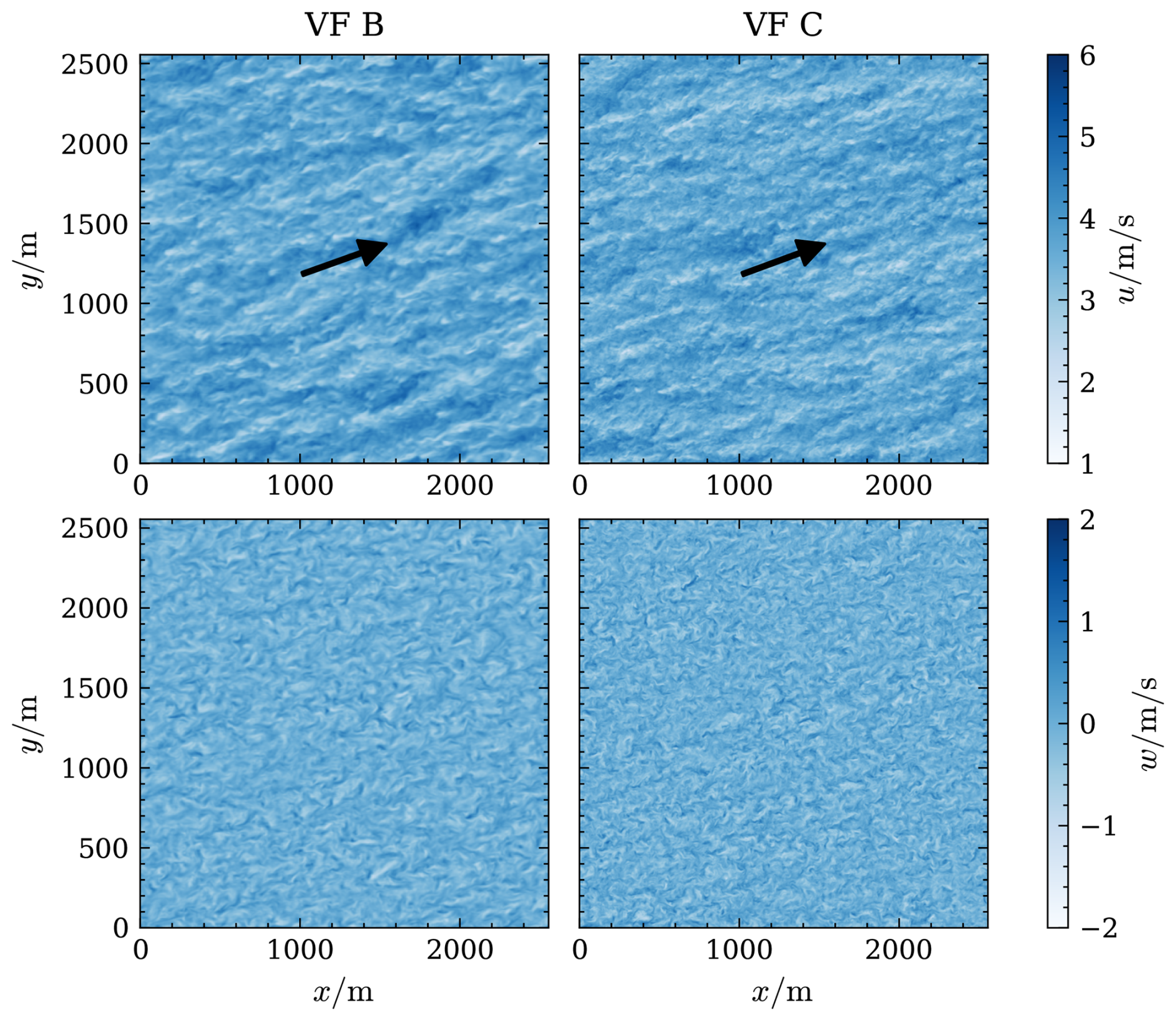
Figure 1 Instantaneous velocity fields of the CNBL case for grids B (left) and C (right). Horizontal wind speed (top) and vertical velocity (bottom) in the plane at z = 37 m are shown. The black arrow in the top row indicates the average wind direction in the plane.

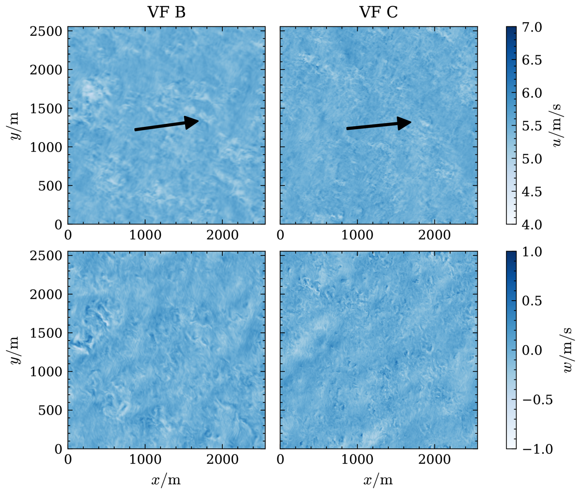
Figure 2 Instantaneous velocity fields of the CNBL case for grids B (left) and C (right). Horizontal wind speed (top) and vertical velocity (bottom) in the plane at z = 333 m are shown. The black arrow indicates the average wind direction in the plane.

We provide a qualitative impression of the simulation in Figs. 1 and 2, where we show instantaneous horizontal wind speed and vertical velocity at z = 35 m and z = 333 m, equivalent to 10 % and 90 % of the boundary layer height, respectively. Similar plots are shown in Berg et al. (2020). At the lower height we see the dominance of small-scale turbulent structures in both horizontal and vertical directions, as expected due to the proximity of the wall. At higher resolution we can observe that smaller scales are resolved. Close to the inversion height, we find much fewer small scales; instead, larger structures dominate. Comparing the direction of the mean horizontal velocity indicated by the black arrow, we observe the expected veer.

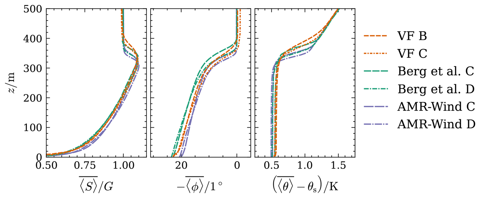
Figure 3 Vertical profiles of averaged velocity (left), wind veer (center), and temperature (right) of the CNBL reference case.

Moving to a more quantitative analysis, we show the horizontal averages of wind speed S, wind direction ϕ, and potential temperature of our model, referred to as VF, alongside respective results from references in Fig. 3. Overall, we find very good agreement between our results and the references. Within the boundary layer in particular we observe very close agreement in all quantities, indicating that the boundary condition and other models behave correctly. However, we observe that the B grid is not able to properly resolve the upper edge of the capping inversion, resulting in a weaker gradient. This is in line with observations in Berg et al. (2020) and a range of other literature, for example van Heerwaarden et al. (2017). Furthermore, we observe that the wind direction in the free atmosphere is not exactly aligned with the geostrophic wind for the higher-resolution case. This inaccuracy is due to the forcing of the geostrophic wind being very small compared to the streamwise velocity in the free atmosphere. See Appendix E for more details. Nevertheless, the error is small and seems to have a negligible effect on the wind direction below the inversion.

From the averaged results we can compute an inversion height z_i as the height with the maximum temperature gradient. We list our results next to the results reported by Berg et al. (2020) and AMR-Wind in Table 1. Furthermore, we list the friction velocity computed from the wall model. All results agree closely. The inversion height decreases with higher resolution for all solvers. AMR-Wind reports the lowest inversion heights, while our results for grid C are in the middle. We report the lowest friction velocity, while Berg et al. (2020) report the highest. Nevertheless, the results agree within 10 % of each other.

Table 1 Friction velocity and inversion height of the CNBL case compared to references.

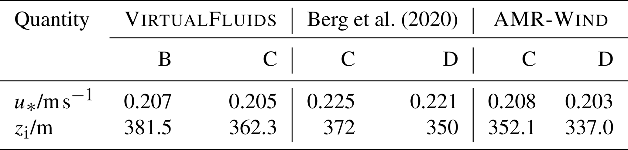
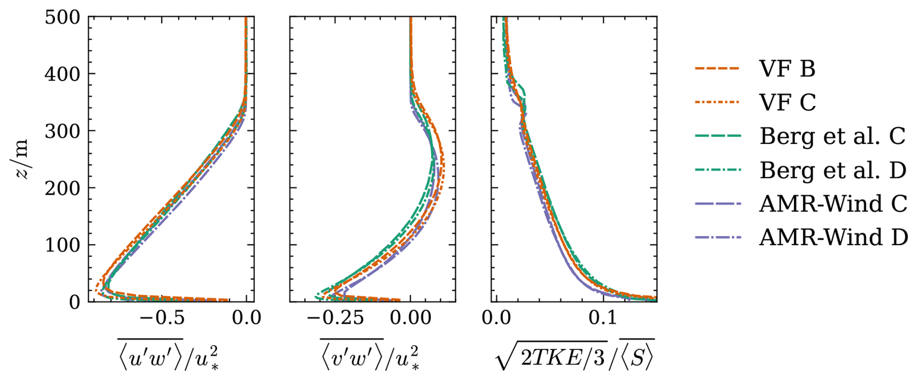
Figure 4 Vertical profiles of resolved vertical momentum flux in the streamwise (left) and lateral (center) directions and resolved turbulence intensity (right) from the CNBL reference case.

We show second-order statistics in Fig. 4, where we present the vertical momentum flux in the streamwise ($u^{\prime }{w}^{\prime }$) and lateral directions ($v^{\prime }{w}^{\prime }$) and turbulence intensity based on the horizontally averaged wind speed, computed as $\sqrt{\mathrm{2}\text{TKE}/\mathrm{3}}/\stackrel{\mathrm{‾}}{\langle S\rangle }$, where $\text{TKE}=\frac{\mathrm{1}}{\mathrm{2}}(\stackrel{\mathrm{‾}}{\langle u^{\prime }{u}^{\prime }\rangle }+\stackrel{\mathrm{‾}}{\langle v^{\prime }{v}^{\prime }\rangle }+\stackrel{\mathrm{‾}}{\langle w^{\prime }{w}^{\prime }\rangle })$ is the resolved turbulence kinetic energy. Again, we find very good agreement with both references. The streamwise flux even shows excellent agreement. We can see the influence of the mismatch in wind direction in the lateral vertical momentum flux, which is slightly too high in the upper region of the boundary layer. The turbulence intensity is slightly higher near the ground than the results from AMR-Wind, while the agreement with the results from Berg et al. (2020) is very close. The prominent increase in turbulence intensity at the inversion height observed in AMR-Wind is significantly less prominent in our results, even at the same resolution.

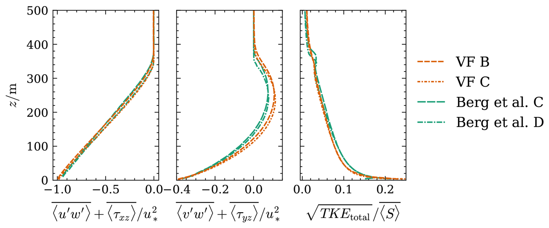
Figure 5 Vertical profiles of total vertical momentum flux in the streamwise (left) and lateral (center) directions and total turbulence intensity (right).

To evaluate the performance of the SGS model in more detail, we present the total flux as the sum of resolved and subgrid-scale fluxes ${\mathit{\tau }}_{ij}={\mathit{\nu }}_e(\frac{\partial u_i}{\partial x_j}+\frac{\partial u_j}{\partial x_i})$ and the total turbulence intensity ${\text{TKE}}_{\text{total}}=\text{TKE}+\frac{\mathrm{1}}{\mathrm{2}}\stackrel{\mathrm{‾}}{\langle {\mathit{\tau }}_{ii}\rangle }$ in Fig. 5. Note that total fluxes are only available from Berg et al. (2020). Again, we find very close agreement with the reference data. Only the lateral flux deviates somewhat from the reference results in the upper half of the boundary layer.

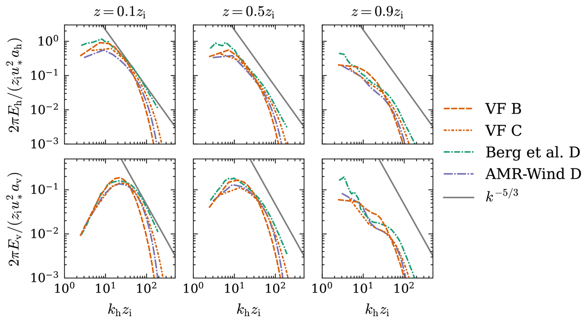
Figure 6 Horizontal (top) and vertical (bottom) spectra at z = 37 m (left), z = 186 m (center), and z = 333 m (right).

Finally, we compare spatial velocity spectra obtained at three different heights (z = 37, 186, and 333 m) in Fig. 6. We compute spectra from horizontal planes following the procedure described in Berg et al. (2020). First, we compute the spectral tensors Φ₁₁, Φ₂₂, and Φ₃₃ from the covariance function $R_{ij}(r_x,r_y,z)=\langle u_i^{\prime }(x,y,z)u_j^{\prime }(x+r_{\mathrm{x}},y+r_{\mathrm{y}},z)\rangle$:

$$\begin{array}{}\text{(35)}& {\mathrm{\Phi }}_{ij}(k_{\mathrm{x}},k_{\mathrm{y}},z)={\displaystyle \frac{\mathrm{1}}{(\mathrm{2}\mathit{\pi }{)}^{\mathrm{2}}}}\iint R_{ij}{e}^{\widehat{\mathrm{1}}(r_{\mathrm{x}}{k}_{\mathrm{x}}+r_{\mathrm{y}}{k}_{\mathrm{y}})}\mathrm{d}{r}_{\mathrm{x}}\mathrm{d}{r}_{\mathrm{y}},\end{array}$$

where $\widehat{\mathrm{1}}$ is the imaginary unit.

Then, we compute the ring-averaged energy in horizontal and vertical spectra E_h(k_h) and E_v(k_h) with $k_{\mathrm{h}}=\sqrt{k_{\mathrm{x}}^{\mathrm{2}}+k_{\mathrm{y}}^{\mathrm{2}}}$:

$$\begin{array}{}\text{(36)}& {\displaystyle }& {\displaystyle }{E}_{\mathrm{h}}\left(k_{\mathrm{h}}\right)={\displaystyle \frac{\mathrm{1}}{\mathrm{2}}}\underset{\mathrm{0}}{\overset{\mathrm{2}\mathit{\pi }}{\int }}{\mathrm{\Phi }}_{\mathrm{11}}(k_{\mathrm{h}},\mathit{\varphi })+{\mathrm{\Phi }}_{\mathrm{22}}(k_{\mathrm{h}},\mathit{\varphi })\mathrm{d}\mathit{\varphi },\text{(37)}& {\displaystyle }& {\displaystyle }{E}_{\mathrm{v}}\left(k_{\mathrm{h}}\right)=\underset{\mathrm{0}}{\overset{\mathrm{2}\mathit{\pi }}{\int }}{\mathrm{\Phi }}_{\mathrm{33}}(k_{\mathrm{h}},\mathit{\varphi })\mathrm{d}\mathit{\varphi }.\end{array}$$

Results are binned into 50 equally sized bins. Wavelengths are normalized with the computed inversion height, and spectra are normalized by $\frac{\mathrm{2}\mathit{\pi }}{z_{\mathrm{i}}{u}_{\ast }{a}_{\mathrm{h}}}$ and $\frac{\mathrm{2}\mathit{\pi }}{z_{\mathrm{i}}{u}_{\ast }{a}_{\mathrm{v}}}$, with $a_{\mathrm{h}}=\mathrm{0.54}(\mathrm{55}/\mathrm{18})a$, $a_{\mathrm{v}}=\mathrm{0.61}(\mathrm{55}/\mathrm{18})a$, and a=0.5, in accordance with Berg et al. (2020). As a final step, we average the spectra computed from 10 time steps to reduce noise.

Our results match the results from AMR-Wind very closely at all heights despite the lower resolution. This demonstrates the lower dissipativity of the cumulant LBM compared to finite-volume solvers. At lower wavenumbers there is also very good agreement with the results from Berg et al. (2020). At high wavenumbers, the LBM is more dissipative than the pseudospectral solver. Close to the inversion height, the small wavenumbers are lower due to the capping inversion, and a characteristic hump is visible in the vertical spectra, which we could accurately reproduce with our solver.

Overall we find very good agreement in all examined quantities with the reference data, even at lower resolutions. In general, the accuracy of the model is positioned between the two reference models. The newly developed surface boundary condition is able to model the wall region accurately in neutral conditions.

Our simulations were carried out using a single NVidia RTX A6000 GPU on a workstation computer. Simulating 1.225 × 10⁵ s with grid B required 2.7 × 10⁴ s of wall time, while the simulation of grid C ran for 4.3 × 10⁵ s, which is approximately a 16-fold increase as expected. Hence, we are able to run full boundary layer simulations using a workstation computer of the order of real time. Further details of the computational efficiency when scaled to multiple GPUs can be found in Appendix D. Compared to isothermal simulations on the same hardware, the computational speed is reduced by around 26 % due to the double-distribution approach, which essentially doubles the memory accessed per node as well as the additional models for Coriolis and buoyancy forces. Future work will combine the different forces and collision kernels to minimize memory access and increase computational efficiency.

3.2 Stably stratified boundary layer

To examine the performance of our model in stable boundary layer simulations, we compare it with the well-known GABLS1 benchmark (Beare et al., 2006). The domain has an extent of 400 m × 400 m × 400 m, with periodic boundaries in the streamwise and lateral directions. The geostrophic wind is set to 8 m s⁻¹ and the Coriolis parameter to 1.39 × 10⁻⁴ 1 s⁻¹. The domain is initialized with a constant velocity equal to the geostrophic wind and a two-layered temperature profile. The lowest 100 m is initialized with a constant temperature θ₀ = 265 K, above which sits an inversion layer with a temperature gradient of 0.01 K m⁻¹. In the lowest 50 m, the temperature is superimposed with random fluctuations with an amplitude of 0.1 K. The surface temperature is also initialized with θ₀, and a constant cooling rate of 0.25 K h⁻¹ is applied. The roughness length is set to z₀ = 0.1 m. The reference temperature is set to 263.5 K, density to 1.3223 kg m⁻³, and gravity to 9.81 m s⁻². A Rayleigh damping layer is used at the top, with the damping factor set to 1.6 × 10⁻³ 1 s⁻¹. We apply the same boundary conditions as in the previous case, but now the surface temperature is prescribed in the surface layer boundary condition. The total simulated time is 9 h, and averages are computed over the last hour. We simulate two grids, one with Δx = 2 m and a finer resolution of Δx = 1 m.

We compare our results to data from the original benchmark and a later publication by Gadde et al. (2021). In the original paper, a number of different models are compared, with a large variety of formulations. Gadde et al. (2021) employ a pseudospectral discretization in horizontal directions and second-order finite differences in the vertical direction and Adam–Bashforth time stepping. They compare three different turbulence models, the Smagorinsky model, the AMD model, and the Lagrangian-averaged scale-dependent model (LASD) (Bou-Zeid et al., 2005). We compare our results only to the results obtained with the Smagorinsky and LASD models since the results differ only marginally between LASD and AMD. Gadde et al. (2021) conduct all simulations at an isotropic resolution of 2.08 m.

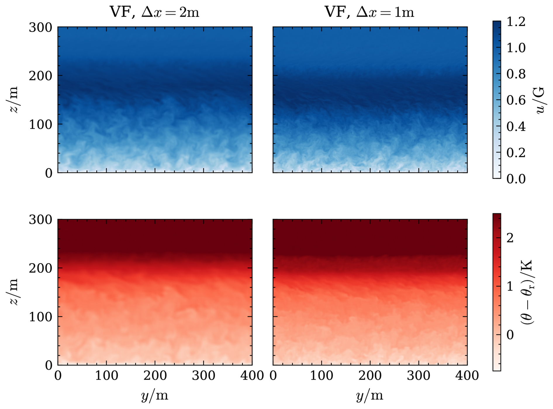
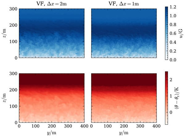
Figure 7 Instantaneous velocity and temperature fields at x = 200 m of simulations of the GABLS1 reference case with both resolutions at t = 9 h.

As with the previous case, we first show an instantaneous view of the simulation in Fig. 7. The capping inversion is clearly visible in the velocity field, exhibiting a super geostrophic wind and high veer. Above the inversion, a clear reduction in turbulence can be observed. At the higher resolution the transition from boundary layer to free atmosphere is sharper, which is discussed in more detail later on. The temperature field shows a stable stratification and the presence of a strong capping inversion.

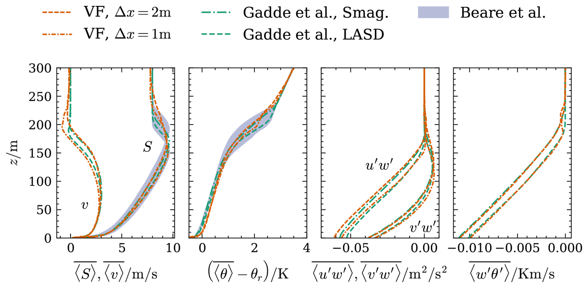
Figure 8 Planar-averaged first- and second-order statistics of the GABLS1 reference case. From left to right: wind speed and lateral velocity, temperature, total momentum fluxes, and total vertical temperature flux. The area covered by all results at 2 m resolution from Beare et al. (2006) is shown as a blue-shaded area.

We show profiles of horizontally averaged quantities of simulating the GABLS1 reference case in Fig. 8. The wind speed below the inversion agrees well with the reference data in both cases. The case with lower resolution exhibits a significantly lower velocity gradient than the higher-resolution case. This is in line with findings from Beare et al. (2006), where simulations at a lower resolution also exhibited this behavior. At the higher resolution, our results match those of Gadde et al. (2021) closely. We find higher negative veer in the inversion layer compared to Gadde et al. (2021), particularly at higher resolution, which also results in higher wind speed in that region. However, there seems to be only a very limited effect on the flow in the boundary layer. The temperature profile at the lower resolution agrees well with the reference data within the boundary layer. In the inversion layer the gradient is slightly lower than that of Gadde et al. (2021) but still well within the range of results from Beare et al. (2006). At the higher resolution we find very good agreement. The vertical momentum fluxes agree very well with the reference results. Only results from Gadde et al. (2021) are available. The vertical temperature fluxes give a similar picture, although they are slightly smaller than the reference data. Furthermore, there exists a small hump in the results from the case with lower resolution. We believe this is connected to the velocity profile, where the top of the inversion had a significantly lower gradient.

Table 2 Friction velocity, boundary layer height, and buoyancy flux of the GABLS1 case.

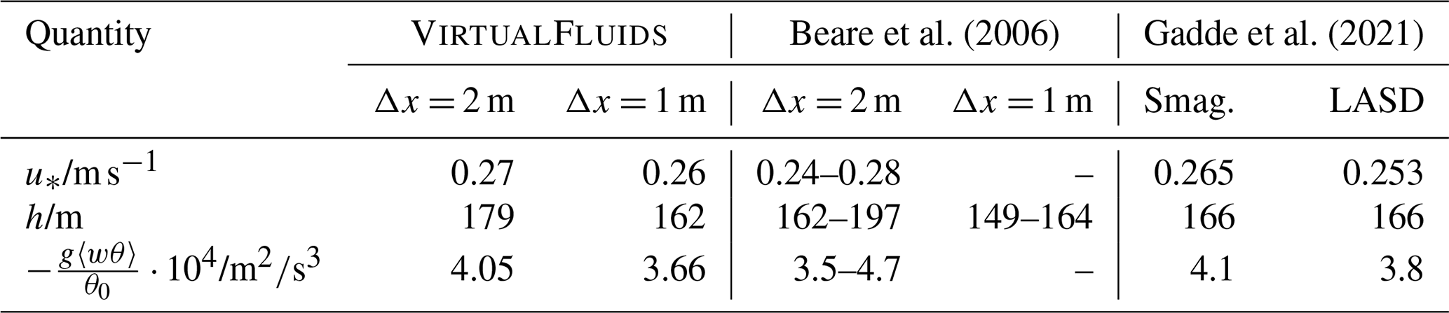
A comparison of some quantities of interest is shown in Table 2. Note that the friction velocity and buoyancy flux are computed from the total fluxes at the second node since this is the node we use as the exchange location for the wall model. We compute the boundary layer height h with the same method used in the references. We first find the height h_0.05 at which the shear stress $\sqrt{(u^{\prime }{w}^{\prime }{)}^{\mathrm{2}}+(v^{\prime }{w}^{\prime }{)}^{\mathrm{2}}}$ is less than 5 % of the wall shear stress and extrapolate by $h=\frac{h_{\mathrm{0.05}}}{\mathrm{0.95}}$.

The friction velocity and buoyancy flux are well within the range of the reference results. This indicates that our wall-modeling approach and boundary condition yield accurate results. The boundary layer height decreases with increasing resolution, as was also observed in Beare et al. (2006).

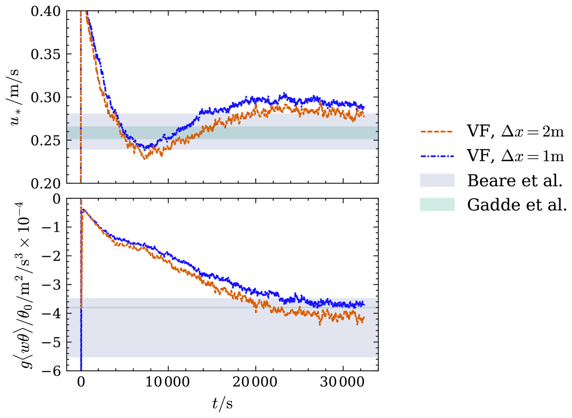
To examine the performance of the new boundary condition in more detail, we show the time evolution of friction velocity and buoyancy flux in Fig. 9. In the initial seconds of the simulation, both quantities exhibit large spikes. The friction velocity first decreases quickly as a boundary layer develops, decreasing shear in the lowest part of the domain. The surface heat flux increases in magnitude as the surface cools, and thus the temperature gradient near the surface increases. Both quantities stabilize towards the end of the simulation, indicating that the simulation has reached a state of equilibrium. This behavior is qualitatively similar to the results reported in Beare et al. (2006) and Sauer and Muñoz-Esparza (2020). Despite varying formulations, different approaches yield similar results near the equilibrium state of the boundary layer.

Figure 9 Time evolution of friction velocity and buoyancy flux of the GABLS1 reference case.

It is worth noting that the reference results also yield a large variation in all predicted quantities, as noted by other studies comparing to this case, e.g., van Heerwaarden et al. (2017) and Sauer and Muñoz-Esparza (2020). Generally, our results within the boundary layer fall well within the range of the results obtained by other solvers, despite the differences in approach, subgrid-scale models, etc. At the top of the boundary layer, our model requires higher resolution than most other solvers to accurately represent the capping inversion. We believe this is caused by the model not representing the temperature gradient accurately enough. One way to improve the model is to further refine the collision operator of the advection–diffusion LBM. In a comparison of different advection–diffusion collision operators, Gruszczyński and Łaniewski-Wołłk (2022) found a two-relaxation time central moment operator to be more accurate than the central moment operator most similar to the one employed here. By introducing more relaxation times, leading-order error terms can be canceled out, and accuracy of the collision operator can be improved, as was done, for example, in Geier et al. (2017).

4 Conclusions

This paper presents a novel method for conducting large-eddy simulation of thermally stratified atmospheric boundary layers using the double-distribution function (DDF) lattice Boltzmann method (LBM) in a GPU-resident solver. Very few applications of the LBM to stratified atmospheric boundary layers have been presented in the literature so far, and this work comprises the first application of a DDF approach to such flows in conjunction with employing GPUs. We give a thorough description of our methodology for the simulation of the bulk flow, present a novel boundary condition to use a combined wall model for wall shear stress and heat flux prescribed by Monin–Obukhov similarity theory, and present other models implemented in the GPU-resident LBM solver VirtualFluids in order to simulate stratified atmospheric boundary layers, including horizontally averaged buoyancy, Coriolis force, and Rayleigh damping layer.

We test our model in simulations of conventionally neutral and stably stratified boundary layers. Simulations of the conventionally neutral boundary layer agree very well with reference data obtained with both pseudospectral and finite-volume methods. At a coarse resolution of 7 m, the inversion layer can not be represented accurately. At a finer resolution of 3.5 m, the results match closely with the reference data at twice the resolution obtained with pseudospectral and finite-volume methods. Second-order statistics also agree very well. The spectra obtained at three heights show that the LBM exhibits excellent spectral properties and has lower diffusion than the finite-volume solver at higher resolution. Damping of vertical motions near the inversion layer is also clearly present.

Simulations of the stably stratified GABLS1 reference case also yield satisfactory results. The proposed boundary condition is able to properly reproduce the friction velocity and buoyancy flux at the wall. The boundary layer height agrees with results obtained at the same resolution.

A general shortcoming of the model is its inability to correctly reproduce the direction of the geostrophic wind, and this discrepancy grows with increasing resolution. However, we find that this does not affect the results in the boundary layer, and the misalignment is small. Overall, we achieve satisfactory accuracy for both cases. The method exhibits the expected behavior, generally being more accurate than a second-order finite-volume method, but not as accurate as a pseudospectral approach.

The present model exhibits excellent computational efficiency. All simulations, even the highly resolved neutral boundary layer with ≈ 140 million nodes, are carried out on a single graphics card. At a coarse resolution of Δx = 7 m, the simulation is carried out 4.5 times faster than real time. Increasing resolution to Δx = 3.5 m results in a simulation at 0.28 real time.

This article comprises a model for an empty boundary layer with flat terrain. Future work will focus on implementing a precursor–successor setup to simulate wind farms. One of the limitations of our model is that the surface layer boundary condition is only formulated for straight walls. As noted by Asmuth et al. (2021), an extension of the inverse momentum exchange method is possible but not available as of yet. Nevertheless, this work represents an important step for the lattice Boltzmann method and CFD in general towards simulations of stratified boundary layers while fully leveraging the computational efficiency of GPUs. It represents one of the most cost-effective and fastest methods available to conduct LES of such complexity. The reduction in computational cost benefits researchers in many ways, from reducing development time to enabling larger parameter studies. Furthermore, a reduction in computational cost is crucial for enabling industrial application of LES, for example in the wind energy sector. That way, manufacturers, developers, and operators can take into account the complex behavior of the atmospheric boundary layer and reduce model uncertainties, ultimately reducing the cost of electricity.

Appendix A: Unsuccessful preliminary studies

The development of this model was rich with paths that led us nowhere, as is often the case when developing a new model. We want to record some of those paths in the hope that others might learn to either avoid those paths or will see where we went wrong and will be able to tell us what we should have done instead.

A1 Hybrid finite-difference scheme

We first tried to implement a hybrid solver by using finite differences for the advection–diffusion problem. The hybrid method has a number of benefits. The finite-difference approach is much simpler and much more well known; hence there is also more literature on the topic. Furthermore, it requires significantly less memory while also yielding higher computational performance. Hence it is used in a number of other thermal LBM models, for example Onodera et al. (2021) and Feng et al. (2021). Results for the canonical test cases looked very promising, so we decided to pursue this direction further. However, when we simulated the atmospheric boundary layer, we could never avoid spurious oscillations that ultimately degraded the simulation, particularly at the top of the inversion layer. We implemented a variety of approaches, beginning with central differences and Euler forward time stepping. We refined our approach, using a variety of different finite-difference schemes, such as the second-order upwind scheme, the MUSCL scheme (Van Leer, 1977), the QUICK and QUICKEST schemes (Leonard, 1979), and the mixed fourth-order central difference and QUICK schemes. We also tried a second-order Adam–Bashforth time integration but all to no avail. At this point we pivoted to a DDF approach that was already implemented in VirtualFluids since adding even higher-order approaches did not seem promising. As of yet it is unclear what the differences were in our approach compared to, for example, the model implemented in ProLB (Feng et al., 2021). On the one hand, we use a much less diffusive collision operator; thus oscillations are not damped as much. On the other hand, no other study actually simulates a capping inversion, where the oscillations originated from our simulations. Furthermore, there is very little literature concerning this issue. We speculate that the instabilities occur due to the differences in stencil/lattice. The lattice Boltzmann method only accesses the direct neighbors, while all the higher-order methods require information from the second neighbor as well; thus information can travel at different speeds. As this was not the aim of this work, we did not explore this direction further.

A2 Reference temperature

To improve the numerical precision, the populations g_ικλ are set so that $\mathit{\theta }-{\mathit{\theta }}_{\mathrm{m}}=\sum g_{\mathit{\iota }\mathit{\kappa }\mathit{\lambda }}$. The choice of the reference temperature θ_m is crucial to improve the accuracy of the simulation. A naïve choice would be to either set it to the reference temperature θ_r or the surface temperature θ₀; however we found that oscillations tended to originate from areas where the temperature is far away from θ_m. We found that the best choice was usually to set θ_m to a value of the temperature in the inversion layer.

Appendix B: Boundary condition fluid

We set a slip boundary condition using a similar method to the one used to set the flux boundary condition. At the uppermost fluid node, we compute the velocity from Eq. (7) and then compute the tangential velocity with

$$\begin{array}{}\text{(B1)}& u_i^{\mathrm{t}}=u_i-\left(u_j{n}_j\right)n_i.\end{array}$$

Then we apply the bounce-back rule:

$$\begin{array}{}\text{(B2)}& f_{\stackrel{\mathrm{‾}}{\mathit{\iota }\mathit{\kappa }\mathit{\lambda }}}=f_{\mathit{\iota }\mathit{\kappa }\mathit{\lambda }}-\mathrm{2}\mathit{\rho }{w}_{\mathit{\iota }\mathit{\kappa }\mathit{\lambda }}{\displaystyle \frac{u_i{c}_{\mathit{\iota }\mathit{\kappa }\mathit{\lambda },i}}{c_{\mathrm{s}}^{\mathrm{2}}}}.\end{array}$$

At the bottom boundary we employ the iMEM approach from Asmuth et al. (2021). We want to give a few clarifications and correct some misprints in the original publication. Recall that the momentum transferred from the fluid to the wall is

$$\begin{array}{}\text{(B3)}& \mathrm{\Delta }{p}_{\mathit{\iota }\mathit{\kappa }\mathit{\lambda },i}=(f_{\mathit{\iota }\mathit{\kappa }\mathit{\lambda }}+f_{\stackrel{\mathrm{‾}}{\mathit{\iota }\mathit{\kappa }\mathit{\lambda }}})c_{\mathit{\iota }\mathit{\kappa }\mathit{\lambda },i}.\end{array}$$

Hence, the total force exerted onto the wall by the fluid is

$$\begin{array}{}\text{(B4)}& F_i={\displaystyle \frac{\mathrm{\Delta }{x}^{\mathrm{3}}}{\mathrm{\Delta }t}}\sum _{\mathit{\iota }\mathit{\kappa }\mathit{\lambda }\in \mathrm{\Gamma }}\mathrm{\Delta }{p}_{\mathit{\iota }\mathit{\kappa }\mathit{\lambda },i},\end{array}$$

where Γ is the set of all links cutting the wall. From the wall model we compute the force acting on the wall from the wall shear stress

$$\begin{array}{}\text{(B5)}& F_i={\mathit{\tau }}_i^{\mathrm{w}}\mathrm{\Delta }{x}^{\mathrm{2}}.\end{array}$$

We now seek a wall velocity u^w such that the bounce-back rule in Eq. (B2) results in the correct force. To that end, we split the force into two components, the force due to the population and due to the wall velocity, F^f and $F^{u_{\mathrm{w}}}$:

$$\begin{array}{}\text{(B6)}& {\displaystyle }& {\displaystyle }{F}_i^{\mathrm{f}}={\displaystyle \frac{\mathrm{\Delta }{x}^{\mathrm{3}}}{\mathrm{\Delta }t}}\sum _{\mathit{\iota }\mathit{\kappa }\mathit{\lambda }\in \mathrm{\Gamma }}{c}_{\mathit{\iota }\mathit{\kappa }\mathit{\lambda },i}(f_{\mathit{\iota }\mathit{\kappa }\mathit{\lambda }}+f_{\stackrel{\mathrm{‾}}{\mathit{\iota }\mathit{\kappa }\mathit{\lambda }}}),\text{(B7)}& {\displaystyle }& {\displaystyle }{F}_i^{u_{\mathrm{w}}}=-{\displaystyle \frac{\mathrm{\Delta }{x}^{\mathrm{3}}}{\mathrm{\Delta }t}}\sum _{\mathit{\iota }\mathit{\kappa }\mathit{\lambda }\in \mathrm{\Gamma }}\mathrm{2}\mathit{\rho }{w}_{\mathit{\iota }\mathit{\kappa }\mathit{\lambda }}{c}_{\mathit{\iota }\mathit{\kappa }\mathit{\lambda },i}{\displaystyle \frac{u_j{c}_{\mathit{\iota }\mathit{\kappa }\mathit{\lambda },j}}{c_{\mathrm{s}}^{\mathrm{2}}}}.\end{array}$$

Thus, $F_i^{u_{\mathrm{w}}}=F_i-F_i^{\mathrm{f}}$, resulting in a system of equations that needs to be solved for u^w. For the case of a straight wall at the bottom, the solution is

$$\begin{array}{}\text{(B8)}& {\mathit{u}}^{\mathrm{w}}=-{\displaystyle \frac{\mathrm{3}{c}_{\mathrm{s}}^{\mathrm{2}}}{\mathit{\rho }}}{\displaystyle \frac{\mathrm{\Delta }{t}^{\mathrm{2}}}{\mathrm{\Delta }{x}^{\mathrm{4}}}}{\left(\mathrm{3}{F}_{\mathrm{1}}^{u_{\mathrm{w}}},\mathrm{3}{F}_{\mathrm{2}}^{u_{\mathrm{w}}},F_{\mathrm{3}}^{u_{\mathrm{w}}}\right)}^{\mathrm{T}}.\end{array}$$

Appendix C: Convergence study

To determine the order of convergence of the advection–diffusion equation numerically, we simulate the advection–diffusion of a Gaussian hill of concentration. Note that in this case, θ is a passive scalar. The initial field of concentration θ is described by Krüger et al. (2017, p. 322):

$$\begin{array}{}\text{(C1)}& \mathit{\theta }(\mathit{x},t=\mathrm{0})={\mathit{\theta }}_{\mathrm{0}}\exp -{\displaystyle \frac{{\left|\mathit{x}-{\mathit{x}}_{\mathrm{0}}\right|}^{\mathrm{2}}}{\mathrm{2}{\mathit{\sigma }}_{\mathrm{0}}}}.\end{array}$$

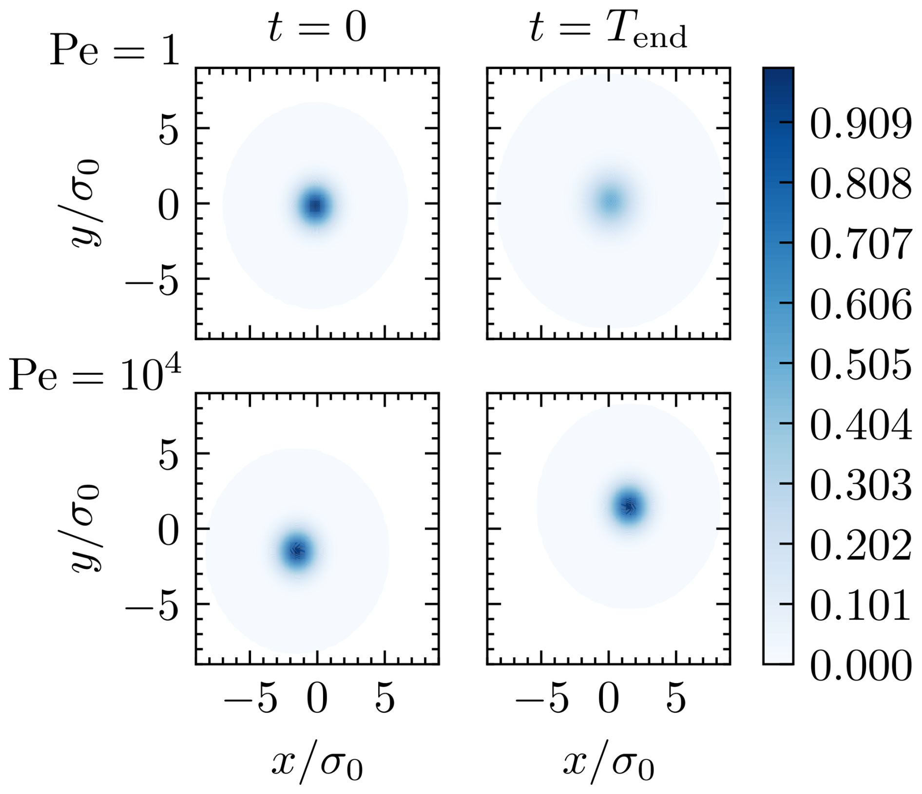
Figure C1 Analytical solution for the concentration in the test case of a Gaussian hill of concentration, projected onto the x–y plane. In the white region concentration θ≤ 1 × 10⁻¹⁰.

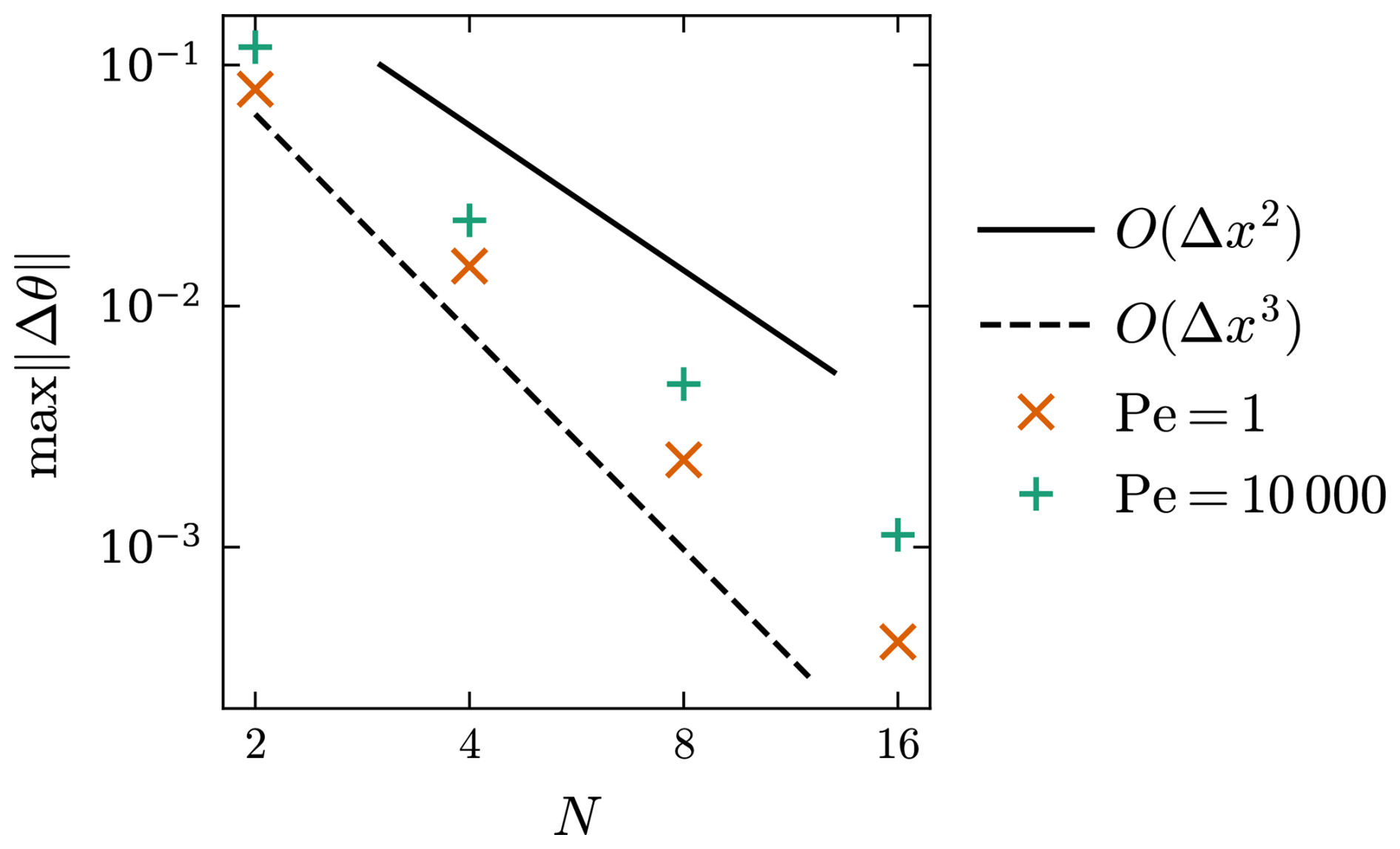
Figure C2 Maximum error Δθ of the numerical results of simulating the advection–diffusion of a Gaussian hill of concentration.

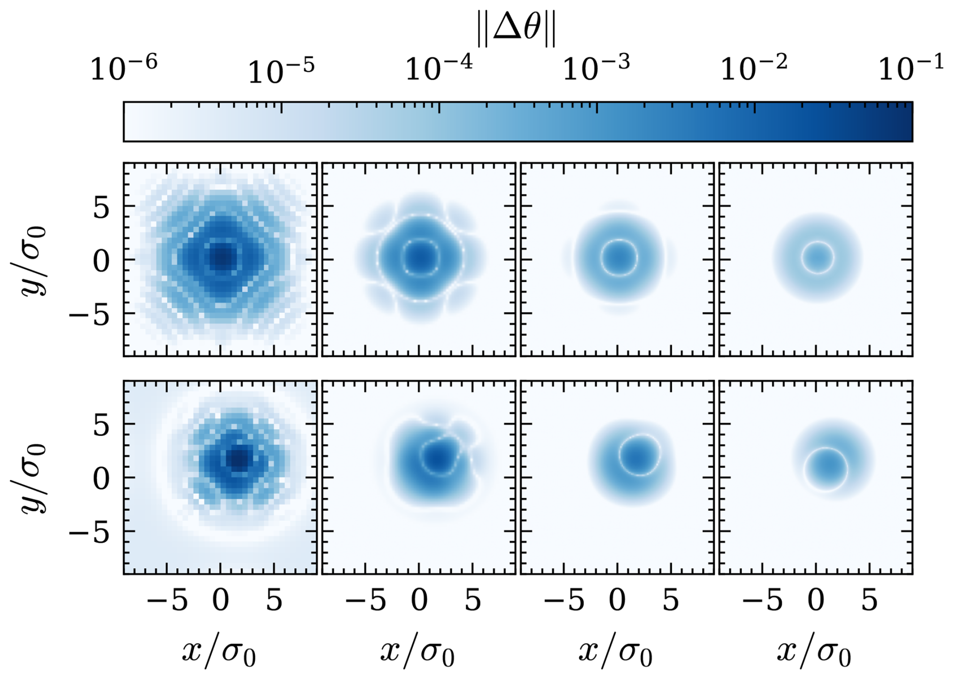
Figure C3 Absolute difference between analytical and numerical solution of the Gaussian hill of concentration at t=T_end. The top row shows the case with Pe=1 and the bottom row the case with Pe=10⁴. Resolution increases from left to right.

Under a constant advection velocity u,

$$\begin{array}{}\text{(C2)}& \mathit{\theta }(\mathit{x},t)={\displaystyle \frac{{\mathit{\sigma }}_{\mathrm{0}}^{\mathrm{2}}}{{\mathit{\sigma }}_{\mathrm{0}}^{\mathrm{2}}+{\mathit{\sigma }}_D^{\mathrm{2}}}}{\mathit{\theta }}_{\mathrm{0}}\exp -{\displaystyle \frac{{\left|\mathit{x}-{\mathit{x}}_{\mathrm{0}}-\mathit{u}t\right|}^{\mathrm{2}}}{\mathrm{2}({\mathit{\sigma }}_{\mathrm{0}}^{\mathrm{2}}+{\mathit{\sigma }}_D^{\mathrm{2}})}}\end{array}$$

is a solution for the advection–diffusion equation

$$\begin{array}{}\text{(C3)}& {\displaystyle \frac{\partial \mathit{\theta }}{\partial t}}+\mathit{u}\cdot {\displaystyle \frac{\partial \mathit{\theta }}{\partial \mathit{x}}}={\displaystyle \frac{\mathrm{1}}{\mathit{Pe}}}{\displaystyle \frac{{\partial }^{\mathrm{2}}\mathit{\theta }}{\partial {\mathit{x}}^{\mathrm{2}}}},\end{array}$$

with ${\mathit{\sigma }}_D=\sqrt{\mathrm{2}Dt}$, the Peclét number $\mathit{Pe}=\frac{{\mathit{\sigma }}_{\mathrm{0}}U}{D}$, and $\mathit{u}=[\mathrm{1},\mathrm{1},\mathrm{1}{]}^{\mathrm{T}}U$. We conduct a convergence study for a diffusion-dominated problem (Pe=1) and an advection-dominated problem (Pe=10⁵). We vary $N={\mathit{\sigma }}_{\mathrm{0}}/\mathrm{\Delta }x=\mathrm{2},\mathrm{4},\mathrm{8},\mathrm{16}$, while we keep σ₀=1 and Δt=1 constant. In the case of Pe=1, we set the diffusivity in lattice units $\stackrel{\mathrm{̃}}{D}=D\frac{\mathrm{\Delta }t}{\mathrm{\Delta }{x}^{\mathrm{2}}}=\mathrm{0.01}$, and we simulate until $T_{\text{end}}=\mathrm{0.3}\frac{{\mathit{\sigma }}_{\mathrm{0}}}{U}$ is reached. In the case of Pe=10⁵, $\stackrel{\mathrm{̃}}{D}$ = 1 × 10⁻⁵ and $T_{\text{end}}=\mathrm{3}\frac{{\mathit{\sigma }}_{\mathrm{0}}}{U}$. In both cases the domain has a size of $\mathrm{18}{\mathit{\sigma }}_{\mathrm{0}}\times \mathrm{18}{\mathit{\sigma }}_{\mathrm{0}}\times \mathrm{18}{\mathit{\sigma }}_{\mathrm{0}}$. To optimally utilize the simulation domain, we set ${\mathit{x}}_{\mathrm{0}}=-T_{\text{end}}U/\mathrm{2}$. The analytical solutions for both Peclét numbers at t=0 and t=T_end are shown in Fig. C1. The results of the convergence test for both Peclét numbers can be found in Fig. C2. The results clearly show a convergence rate slightly above second order in both cases, as expected. More precisely, we compute a convergence rate of 2.5 and 2.2 for Pe=1 and Pe=10⁵, respectively. A more detailed view of the error can be found in Fig. C3, where we show the absolute difference between the analytical and numerical solution. We see that in both cases, errors decrease with higher resolution and that the error is symmetric in the diffusion-dominated case, while the advection case exhibits errors aligned with the direction of advection. We also see that errors become negligibly small towards the boundaries of the domain, so the domain was chosen to be large enough to not affect the results.

Appendix D: Scaling study

Table D1 $\frac{T_{\text{wall}}}{T_{\text{sim}}}$ for all cases of the scaling study.

We conduct both a weak and a strong scaling study of the model based on the neutrally stratified test case with grid C (Δx = 3.5 m). However, we want to emphasize that the model in its current state has not yet been optimized for performance and not at all for multi-GPU performance. These improvements will be a topic of future studies.

The study is conducted on the Dardel supercomputer from 1 to 8 GPUs. Each node has 4 Nvidia GH200 Grace Hopper superchips with 120 GB memory each. The domain is partitioned into equally sized subdomains along the streamwise direction. This was found to be the optimal partitioning strategy for this case. Each case is run for 100 s of simulation time, and the wall time T_wall of the longest-running process is recorded. On a single GPU, the domain has a size of 3060 m × 3600 m to fully use the available memory of the card.

For the weak scaling study we simply extended the domain to 7200 m × 3600 m, 7200 m × 7200 m, and 14 400 m × 7200 m for 2, 4, and 8 GPUs, respectively. The reference wall time T_wall,ref for all simulations is the wall time of the single-GPU case.

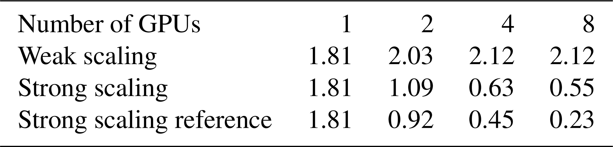
In the strong scaling study, we partition the same domain into smaller and smaller subdomains. However, if the subdomain becomes too small, the GPU is not saturated any more, and the parallel efficiency decreases. We therefore ran a reference case for each case of the scaling study where the domain had the same size as one subdomain and use the wall time of that case as T_wall,ref. By normalizing in this manner, ideal scaling corresponds to a constant ratio of $T_{\text{wall},\text{ref}}/T_{\text{wall}}$.

The wall time for each case can be found in Table D1, and the results of both scaling studies are shown in Fig. D1.

Figure D1 Results of the strong and weak scaling study from 1 to 8 GPUs.

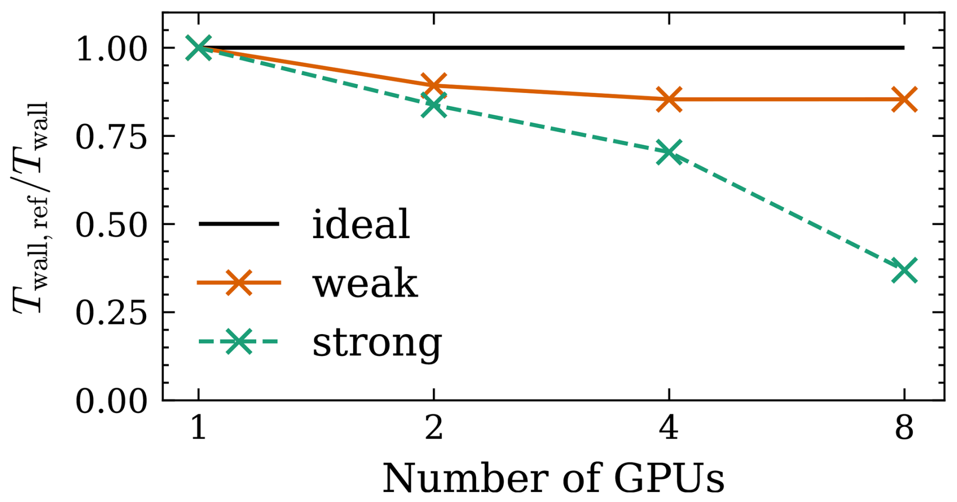
The weak scaling efficiency of the model is already good. Even at 8 GPUs the efficiency is still at 85 %, indicating that the model is suitable for large-scale computation. We also find that the efficiency does not noticeably decrease from 4 to 8 GPUs. We observe that the model does not scale as well in the strong scaling study. On the one hand, this can be explained simply by the square-cube law; i.e., the volume of the subdomains shrinks faster than the surface. The communication hiding implemented in VirtualFluids becomes less effective for smaller subdomains; see Geier et al. (2025). This problem is exacerbated due to the planar averaging in Eq. (5), which also requires inter-GPU communication and becomes less efficient when partitioned along the streamwise direction. Nevertheless, the efficiency is still around 35 %. Comparing these results with Min et al. (2024), we find that our model has comparable scaling efficiency in the weak scaling study, although we use significantly fewer GPUs.

Appendix E: Unit conversion in LBM and its effect on small forces

The LBM relies on non-dimensionalizing all quantities with grid size Δx, time step size Δt, and reference density ρ₀. Furthermore, recall that $\frac{\mathrm{\Delta }x}{\sqrt{\mathrm{3}}\mathrm{\Delta }t}=c_{\mathrm{s}}=\frac{V_{\mathrm{0}}}{\text{Ma}}$, which we have kept constant. Thus, velocities in SI units are scaled as $\stackrel{\mathrm{̃}}{u}=\frac{u}{C_{\mathrm{u}}}$, where $C_{\mathrm{u}}=\frac{\mathrm{\Delta }x}{\mathrm{\Delta }t}=\text{const}$, and $\stackrel{\mathrm{̃}}{u}$ is the velocity in LB units. Forces, however, are scaled as $\stackrel{\mathrm{̃}}{f}=\frac{f}{C_{\mathrm{f}}}$, with $C_{\mathrm{f}}={\mathit{\rho }}_{\mathrm{0}}\frac{\mathrm{\Delta }x}{\mathrm{\Delta }{t}^{\mathrm{2}}}={\mathit{\rho }}_{\mathrm{0}}\frac{\mathrm{3}{c}_{\mathrm{s}}^{\mathrm{2}}}{\mathrm{\Delta }x}$ (Krüger et al., 2017, Chap. 7). Therefore, non-dimensionalized forces decrease with grid spacing. In the cumulant LBM, forces are only applied via Eq. (7) (Geier et al., 2015). Therefore, the result of the addition becomes less accurate with increasing resolution, since the contribution of the force can not be represented in finite-precision floating point numbers. This becomes particularly important for small forces, such as the Coriolis force, and when using single-precision floating point numbers. We have tried the Kahan summation algorithm (Kahan, 1965) as a remedy but that did not improve the results.