Aerodynamic analysis of standard variable-speed torque control in complex terrain

Wind energy projects in complex terrain are often associated with high uncertainties regarding the expected power performance. These uncertainties are mostly attributed to difficulties in obtaining reliable wind speed estimates. Two additional factors are that the physical limits of energy extraction vary in these cases and that the employed wind turbine might operate differently than expected in these conditions. This study addresses these two factors with the goals of identifying the dominant factor influencing power performance and improving understanding of how a turbine controller operates in flow conditions for which it was not calibrated. For this purpose, Reynolds-averaged Navier–Stokes (RANS) simulations of a wind turbine modeled as an actuator disk (AD) subject to a neutral atmospheric inflow are performed. The influence of the turbine position relative to a quasi-two-dimensional Gaussian hill with varying dimensions on the maximum power performance and on the response of a torque controller in region 2 of the power curve is investigated. For two cases analyzed in detail, it is found that when the turbine is located at the foot of the hill, the maximum power coefficient increases by 2.46 %, while it decreases by 18.25 % on top of the hill. As a consequence, when placing wind turbines on elevated locations, the power does not scale with the cube of the increase in wind speed. The controller maintains a constant local power coefficient, i.e., the power coefficient based on the disturbed rotor-plane velocity. This local power coefficient does not necessarily coincide with the optimal power coefficient defined using the undisturbed wind speed. As a result, the controller does not track optimal performance when the relationship between undisturbed and disturbed wind speed differs from the calibration conditions, such as when a controller tuned for flat terrain is applied in complex terrain. In the present study, this mismatch leads to a maximum power loss of 1.96 %. Overall, this study sheds light on the interpretation of wind turbine performance results in complex terrain and helps shape efforts to reduce prediction uncertainties for future onshore wind projects in complex terrain.

1 Introduction

Wind turbine operation can be roughly divided into three regions depending on the undisturbed wind speed. In region 1, no power is extracted; in region 2, the primary objective is to maximize power performance; and in region 3, the power generation is kept constant. Generally, the generator torque and the collective blade pitch are used to control the turbine (Abbas et al., 2022), and since the undisturbed wind speed can be difficult to evaluate, the generator speed often serves as a control input. Control tuning is usually based on aeroelastic simulations of the turbine of interest, as has been done, for example, for the NREL 5 MW reference wind turbine (RWT) (Jonkman et al., 2009) or the DTU 10 MW RWT (Bak et al., 2013).

In region 2, constraints on performance optimization often stem from load considerations, where optimum performance is sacrificed for a reduction in loads. However, this work is only concerned about maximum performance in region 2 and hence does not consider loads.

During the identification of the points of maximum performance in aeroelastic simulations, the mean flow is usually assumed to vary over the rotor area due to vertical shear and yaw misalignment but is assumed to be uniform in the streamwise direction. These conditions are fulfilled in flat terrain but not in complex terrain, where topography induces significant streamwise flow variations due to hills, elevations, ramps, and other features. An analysis of a simplified analytical model capturing the effects of acceleration induced by complex terrain has shown that, in such conditions, the maximum performance and the point of optimal operation of a constantly loaded actuator disk (AD) change (Zengler et al., 2025a). This raises the question of whether a controller tuned in flat-terrain conditions still tracks optimal performance in region 2 when operating in complex terrain.

In general, recent research has shown that using only local rotor quantities, such as the undisturbed wind speed at the turbine position, is insufficient to quantify the extractable energy, but also the streamwise development of the undisturbed wind speed must be taken into account (Troldborg et al., 2022; Zengler et al., 2024; Revaz and Porté-Agel, 2024). In other words, both the turbine's location and the local development of the flow field affect the power performance quantified by the power coefficient. A streamwise acceleration of the flow leads to an increase of the power coefficient, while a deceleration leads to a decrease (Dar et al., 2023). Besides the simple model mentioned above, several other models based on conservation equations have been developed to describe this effect (Cai et al., 2021; Dar et al., 2025, 2026).

Studies on wind turbine performance in complex terrain often rely on specific controllers without actively investigating the influence of the chosen controller and its tuning on performance. In a large-eddy simulation (LES) study investigating the influence of a hill on the power performance of individual turbines and wind farms, Liu and Stevens (2022) scale the rotor forces based on the disturbed disk-averaged velocity and a prescribed modified thrust coefficient based on the disturbed disk-averaged velocity as proposed by Meyers and Meneveau (2010). This thrust coefficient is determined in advance and does not appear to be tuned to maximize power extraction in the investigated cases. Revaz and Porté-Agel (2024) and Dar et al. (2025) do not explicitly state the controller used in their LES studies of wind turbines in streamwise non-uniform flows, but it seems to be the one described by Wu and Porté-Agel (2015), which sets the rotor speed based on a prescribed relation between torque and rotor speed in an iterative procedure. In both studies, the tip-speed ratio, necessary to evaluate the turbine's operational state, is not reported. Mishra et al. (2024) use the reference open-source controller (ROSCO) developed by Abbas et al. (2022) for their study of a wind turbine ahead of a quasi-two-dimensional hill without stating which of the two control strategies available in the controller for region 2 is used. Prospathopoulos et al. (2010) performed Reynolds-averaged Navier–Stokes (RANS) simulations of an existing wind farm in complex terrain and compared three different ways of controlling the thrust coefficient in terms of how well they match the measured power. They set the thrust coefficient either on the basis of the wind speed 1 diameter upstream of the turbine, from an induction-based estimate, or sequentially by evaluating the undisturbed wind speed when the respective turbine is switched off. The last method showed the best agreement with measurements, but the reasons for this were not evaluated in detail. Overall, these studies show a literature gap regarding how exactly the control choice affects reported power performance. This makes it difficult to draw definite conclusions about performance from these studies, as it is unclear whether the controller continues to maintain its primary control objective of tracking optimal performance in complex terrain.

A common way of controlling a wind turbine in region 2 of the power curve sets the generator torque τ_Gen as a function of the generator speed ω according to τ_Gen=kω², enforcing an equilibrium between generator and rotor torque in steady state (Bossanyi, 2000; Pao and Johnson, 2011; Johnson et al., 2006). This strategy is referred to as k−ω² control and implemented in many turbine controllers and aeroelastic simulation tools, such as ROSCO (Abbas et al., 2022), OpenFAST (Jonkman et al., 2026), Flex5 (Øye, 1996), and HAWC2 (Larsen and Hansen, 2025; Hansen and Henriksen, 2013). The torque constant k can be set based on the optimal power coefficient and tip-speed ratio, which are determined in advance through aeroelastic simulations in flat-terrain conditions as mentioned before.

In a previous work, the analytical model describing the effect of streamwise acceleration on the induction of a uniformly loaded AD (Zengler et al., 2025a) was implemented into a blade element momentum model and coupled with a k−ω² controller. The study showed that, in an accelerating flow, a controller tuned for uniform inflow does not achieve optimal performance (Zengler et al., 2025b). The present study aims to confirm this result in a more realistic setting by performing steady-state RANS simulations of an AD in complex terrain with resolved blade loads. Thus, the analytical flow model representing the acceleration in Zengler et al. (2025b) is replaced by the RANS equations. This allows for more robust conclusions and also addresses quantities such as axial and tangential induction, which have not yet been analyzed in the context of control in complex terrain. In addition, the impact of non-constant power coefficients in complex terrain on the usage of speed-up factors is investigated, yielding a deeper understanding of the expected power increase by placing turbines on elevated position.

The work is structured as follows: Sect. 2 presents the methodology, Sect. 3 presents the results, and Sect. 4 discusses the results and puts them in a broader context. The work concludes in Sect. 5. In Appendices A and B, supporting analytical considerations regarding tangential induction and maximum power performance are provided.

2 Methodology

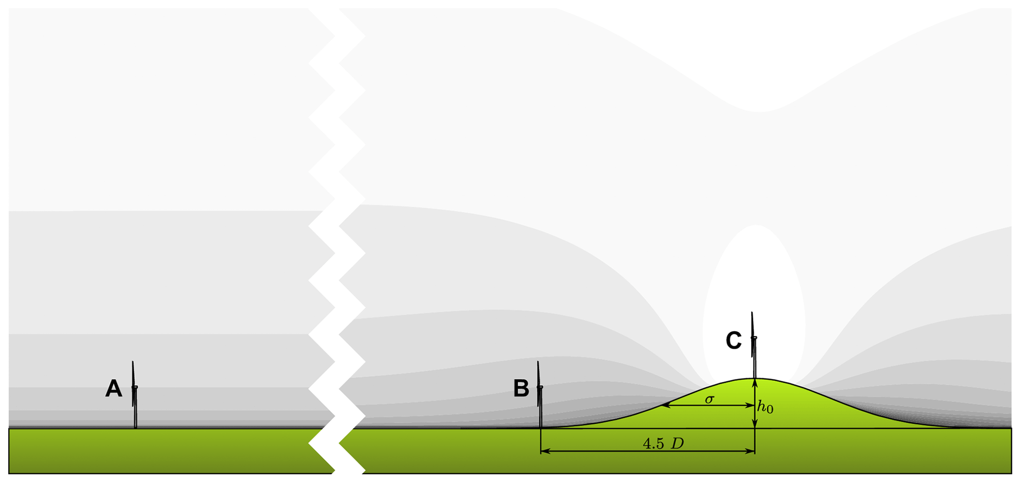
Simulations of a turbine in three different terrain setups are considered, as shown in Fig. 1. In the first case (A), the turbine operates in flat terrain, with no obstacles present. In the second case (B), the turbine is located at the foot of a hill, which accelerates the wake flow. The hill is quasi-two-dimensional, parameterized by a Gaussian function as defined in Sect. 2.4. The direction of the onset wind is perpendicular to the ridge of the hill, resulting in a quasi-two-dimensional flow field when the turbine is not operating. In the last case (C), the turbine is located on the ridge of the hill, which results in a deceleration of the wake. Locations B and C are chosen because they would result in an increase or decrease in performance relative to location A, respectively, which allows for drawing conclusions for both accelerating and decelerating cases. For location C, additional simulations with varying hill height, width, and surface roughness are performed.

The flow setup is similar to a previous work (Zengler et al., 2024), employing RANS simulations of an AD on a quasi-two-dimensional Gaussian hill subject to a neutral atmospheric inflow.

Figure 1 Sketch of the terrain setup with the three considered turbine locations.

2.1 Turbine model

The blade geometries of the DTU 10 MW RWT with a rotor diameter of 178.3 m and a hub height of 119 m are used (Bak et al., 2013). Tower, nacelle, and hub are not included in the simulation.

2.2 k−ω² control

The turbine is controlled by the k−ω² controller in region 2 of the power curve. It relies on the generator's rotational speed, ω, as input. For simplicity, we assume the turbine is a direct-drive turbine, meaning the generator and rotor speeds are equal when losses are neglected. In order to understand the underlying assumptions of k−ω² control, the control law will be derived in the following. We start with the turbine power, which for a given wind speed U_Ref can be calculated as

$$\begin{array}{}\text{(1)}& P={\displaystyle \frac{\mathrm{1}}{\mathrm{2}}}\mathit{\rho }{R}^{\mathrm{2}}\mathit{\pi }{C}_{\mathrm{P}}(\mathit{\lambda },\mathit{\theta },X)U_{\mathrm{Ref}}^{\mathrm{3}},\end{array}$$

with air density ρ; rotor radius R; and power coefficient C_P, which depends on the tip-speed ratio $\mathit{\lambda }=\mathit{\omega }R/U_{\mathrm{Ref}}$, the blade pitch θ, and the location X, as shown by the aforementioned research (Troldborg et al., 2022; Zengler et al., 2024; Revaz and Porté-Agel, 2024). In the following, these dependencies will not be explicitly mentioned. The definition of the reference wind speed U_Ref is provided in Sect. 2.3. The rotor torque is related to the power as

$$\begin{array}{}\text{(2)}& {\mathit{\tau }}_{\mathrm{Rot}}={\displaystyle \frac{P}{\mathit{\omega }}}={\displaystyle \frac{\mathrm{1}}{\mathrm{2}}}\mathit{\rho }{R}^{\mathrm{2}}\mathit{\pi }{C}_{\mathrm{P}}{\displaystyle \frac{U_{\mathrm{Ref}}^{\mathrm{3}}}{\mathit{\omega }}}.\end{array}$$

To design a controller that tracks optimal performance, it is desired to keep the local inflow angles at the blade constant under the conditions where the maximum power coefficient C_P,max is reached. This means that the tip-speed ratio must remain constant under optimal conditions. By substituting $U_{\mathrm{Ref}}=\mathit{\omega }R/{\mathit{\lambda }}_{\mathrm{opt}}$, one obtains (Bossanyi, 2000; Bianchi et al., 2007)

$$\begin{array}{}\text{(3)}& {\mathit{\tau }}_{\mathrm{Rot},\mathrm{opt}}=\underset{k}{\underbrace{{\displaystyle \frac{\mathrm{1}}{\mathrm{2}}}\mathit{\rho }{R}^{\mathrm{5}}\mathit{\pi }{\displaystyle \frac{C_{\mathrm{P},\max }}{{\mathit{\lambda }}_{\mathrm{opt}}^{\mathrm{3}}}}}}{\mathit{\omega }}^{\mathrm{2}},\end{array}$$

where the torque constant k is introduced, representing optimal operational conditions in the given environment. This equation can now be used to set the generator torque τ_Gen as a function of the rotor speed to ensure optimal operation:

$$\begin{array}{}\text{(4)}& {\mathit{\tau }}_{\mathrm{Gen}}=k{\mathit{\omega }}^{\mathrm{2}}.\end{array}$$

The substitution of U_Ref to maintain constant local inflow angles at the blade is essential for understanding how the controller works from an aerodynamic perspective. Of course, the controller does not measure the inflow angles. But maintaining τ_Rot∝ω² is, from an aerodynamic perspective, only possible when aerodynamic forces also scale with the rotor speed squared, which is only the case when local inflow angles at the blades are kept constant. This will become apparent in the course of this paper. In steady state, conservation of angular momentum between the rotor and the generator yields

$$\begin{array}{}\text{(5)}& {\displaystyle }{\mathit{\tau }}_{\mathrm{Gen}}={\mathit{\tau }}_{\mathrm{Rot}}\text{(6)}& {\displaystyle }\iff k{\mathit{\omega }}^{\mathrm{2}}={\displaystyle \frac{\mathrm{1}}{\mathrm{2}}}\mathit{\rho }{R}^{\mathrm{5}}\mathit{\pi }{\displaystyle \frac{C_{\mathrm{P}}}{{\mathit{\lambda }}^{\mathrm{3}}}}{\mathit{\omega }}^{\mathrm{2}}\text{(7)}& {\displaystyle }\iff {\displaystyle \frac{C_{\mathrm{P},\max }}{{\mathit{\lambda }}_{\mathrm{opt}}^{\mathrm{3}}}}={\displaystyle \frac{C_{\mathrm{P}}}{{\mathit{\lambda }}^{\mathrm{3}}}}.\end{array}$$

Thus, the turbine will always track the curve defined by Eq. (7), irrespective of the surrounding flow.

In this work, the k−ω² controller is implemented as part of a five-region generator torque controller as described by Jonkman et al. (2009). In every iteration i of the simulation, ω is updated until convergence based on the conservation of angular momentum of the rotor, which can be written as

$$\begin{array}{}\text{(8)}& {\mathit{\omega }}_{i+\mathrm{1}}={\mathit{\omega }}_i+{\displaystyle \frac{\mathrm{\Delta }t}{J}}\left({\mathit{\tau }}_{\mathrm{Rot},i}-{\mathit{\tau }}_{\mathrm{Gen},i}\right),\end{array}$$

with the time step Δt; the rotor moment of inertia J; and the rotor torque τ_Rot,i, which is extracted from the flow simulation. A low-pass filter for the rotational speed is used in Eq. (8). In steady state, aerodynamic torque and generator torque are balanced, ensuring that in region 2, the turbine tracks maximum power performance in flat terrain. Since steady-state simulations are performed, the dynamic response of the controller is not of interest here, and $\mathrm{\Delta }t/J$ in Eq. (8) is solely tuned to improve solution convergence. The blade pitch is controlled by a proportional-integral (PI) controller as also described by Jonkman et al. (2009), which modifies the blade pitch above rated conditions to maintain rated rotor speed and consequently power. By design, the PI controller saturates below rated conditions at θ_opt.

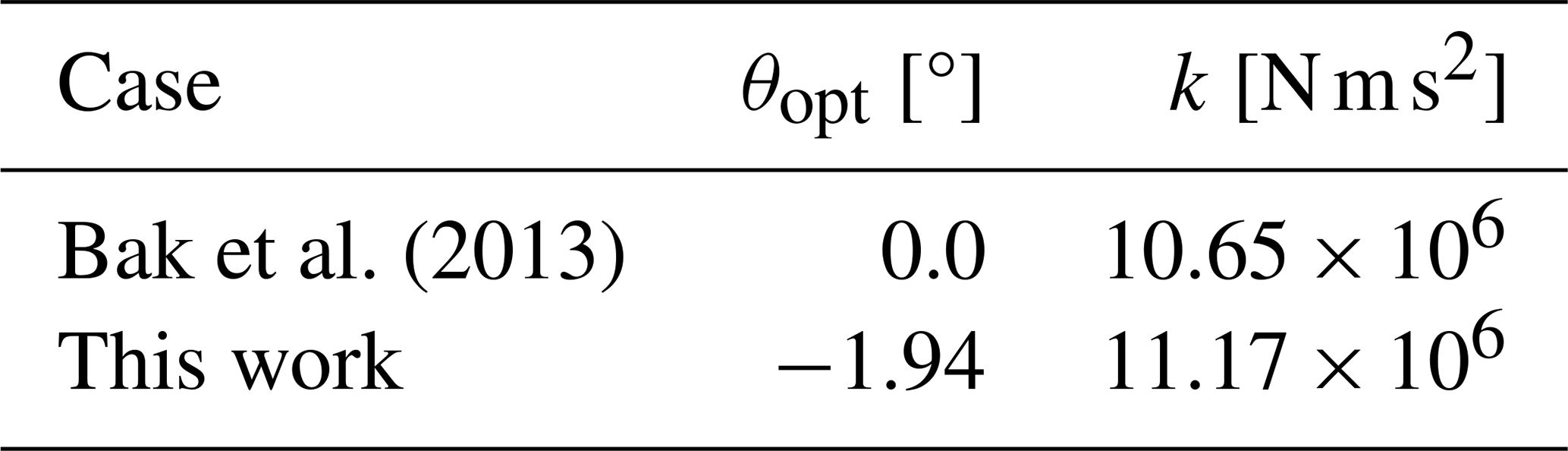
The optimal blade pitch θ_opt, tip-speed ratio λ_opt, and power coefficient C_P,max can be obtained from aeroelastic simulations of the turbine without the flow field being resolved by CFD, as has also been done for the DTU 10 MW RWT by Bak et al. (2013). The optimum identified in this way is not necessarily the same optimum as can be found when resolving the flow field with CFD. In this work, we chose to tune the control constants based on our RANS simulation setup, as shown later in Sect. 3.2. The resulting control constants are listed in Table 1.

Bak et al. (2013)

Table 1 Controller settings investigated within this study. Note that the torque constant for the default control settings from Bak et al. (2013) is adjusted for the generator efficiency of 0.94.

2.3 Reference wind speed and normalization of quantities

We introduce the following decomposition of the mean flow:

$$\begin{array}{}\text{(9)}& u=U+u^{\prime },\end{array}$$

where u is the flow field including the turbine interacting with it, U is the undisturbed flow field, and u^′ quantifies the disturbance by the turbine. The reference wind speed employed throughout this work is the undisturbed rotor-equivalent wind speed, which we calculated as an average not only over height as originally proposed by Wagner et al. (2011), but also over the lateral dimension as

$$\begin{array}{}\text{(10)}& U_{\mathrm{Ref}}=\sqrt[\mathrm{3}]{{\displaystyle \frac{\mathrm{1}}{A_R}}\underset{A_R}{\int }{U}_{\mathrm{R}}^{\mathrm{3}}\mathrm{d}A},\end{array}$$

with U_R being the undisturbed rotor-normal velocity component at the location of the rotor. This approach takes the variation in available kinetic energy over the rotor plane into account and allows for a more accurate assessment of the efficiency of a turbine. However, it does not consider the streamwise development of the undisturbed flow field.

At every turbine location, U_Ref is obtained separately. Therefore, quantities like λ, C_P, and the axial induction a are normalized by the respective local U_Ref evaluated when the turbine is turned off and not by an upstream velocity. By defining the reference wind speed like this, any bias in the performance results due to a change in kinetic energy of the flow induced by the topography between wind speed measurement position and turbine position is avoided. It is also more consistent defining the reference wind speed like this compared to choosing an arbitrary position upstream, where the relation between the wind speed at this position and the turbine position depends on the terrain.

In Sect. 4.3, the case of a turbine placed on top of a hill (location C) is used to analyze the combined effect of the increased kinetic energy at the turbine position and the flow deceleration behind the hill.

2.4 Domain and grid design

The shape of the quasi-two-dimensional Gaussian hill is described by

$$\begin{array}{}\text{(11)}& h=h_{\mathrm{0}}\exp \left(-{\displaystyle \frac{x^{\mathrm{2}}}{\mathrm{2}{\mathit{\sigma }}^{\mathrm{2}}}}\right),\end{array}$$

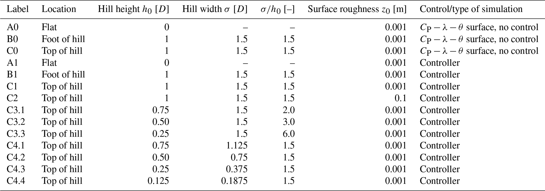
and has, in its standard configuration, a height h₀ of 1 D and a standard width σ of 1.5 D, with D denoting the turbine diameter. When the turbine is located at the foot of the hill (B), it is 4.5 D away from the top of the hill. The surface roughness is 0.001 m, corresponding to a snowy surface (Troen and Petersen, 1989). Due to this low roughness, the flow does not separate behind the crest, leading to a strong deceleration and noticeable impact on the induction (Zengler et al., 2024). The configuration as a whole is chosen because it modifies the flow in the proximity of the AD at a length scale comparable to the rotor size. When characteristic lengths of the hill, such as height or width, are significantly smaller than the turbine, its impact on performance vanishes, and the same holds when the hill is significantly bigger than the turbine (Revaz and Porté-Agel, 2024). Effectively, the turbine is subject to a flow comparable to flat terrain in such cases. The setup is similar in dimensions to other studies (Liu and Stevens, 2022; Mishra et al., 2024; Troldborg et al., 2022) but purposely idealized to investigate the isolated effect of flow acceleration and deceleration. To allow for more general conclusions, three additional sets of simulations of the turbine on top of the hill are performed. In the first set (C2), the surface roughness is changed to 0.1 m. In the second set (C3.X), the hill height is varied, while the width is kept constant, and in the last set (C4.X), both hill height and width are scaled with the same scaling factor, thus keeping the ratio between height and width constant.

An overview of all simulations is listed in Table 2. The simulations are performed in two steps. First, the domain is simulated without the turbine to extract the undisturbed U_Ref at the turbine position. Second, after convergence of the empty domain, the turbine is placed into the domain, and the simulation is run until convergence again to extract the relevant turbine and flow metrics.

Table 2 Simulations conducted within this study. The controller is tuned based on optimal operation obtained from A0.

In all cases, the computational domain is a curvilinear grid with a size of 45 × 18 × 34 D³ in the x, y, and z directions, respectively, which correspond to the streamwise, lateral, and vertical dimensions, respectively. The hill is generated by deforming the bottom surface of a flat domain. In total, the grid has a size of 256 × 192 × 192 = 9.44 × 10⁶ cells. In the turbine region, the mesh is refined with nearly cubic cells with a side length of approximately $D/$32.

The turbine is simulated as an AD, which is represented in the flow domain by a polar grid, and forces are projected onto the computational grid by the actuator shape approach (Réthoré et al., 2014; Troldborg et al., 2015). The tip-loss correction by Glauert is applied, and the disk grid has 17 radial points and 64 azimuthal points.

2.5 Turbulence model, inflow, boundary conditions, and solver

The simulations are performed as RANS simulations using the $k-\mathit{\epsilon }-fp$ model (van der Laan et al., 2015b) as a closure model. The standard model coefficients are left unaltered, and the inflow is described by the analytical log-law solutions for the velocity U, the turbulence kinetic energy k, and the dissipation ε (van der Laan et al., 2015a):

$$\begin{array}{}\text{(12)}& U={\displaystyle \frac{u_{*}}{\mathit{\kappa }}}\log \left({\displaystyle \frac{z+z_{\mathrm{0}}}{z_{\mathrm{0}}}}\right),k={\displaystyle \frac{u_{*}^{\mathrm{2}}}{\sqrt{C_{\mathit{\mu }}}}},\mathit{\epsilon }={\displaystyle \frac{u_{*}^{\mathrm{3}}}{\mathit{\kappa }(z+z_{\mathrm{0}})}},\end{array}$$

with the friction velocity u_* and the von Kármán constant κ. It is important to mention that the level of turbulence intensity is independent of the friction velocity, which is varied in order to change the hub height velocity.

The described inflow is set as a boundary condition at the inlet and at the top of the domain in order to maintain the logarithmic profile in the absence of obstacles. At the outlet, a zero-velocity gradient condition is imposed, and at the bottom, a rough wall boundary condition as described by Sørensen et al. (2007) is used. The lateral boundaries are periodic.

The steady RANS equations are solved using the incompressible finite-volume solver EllipSys3D (Michelsen, 1992, 1994; Sørensen, 1995) using a modified version of the SIMPLEC algorithm to enforce pressure–velocity coupling (Kolmogorov et al., 2015).

2.6 Sensitivity analysis

The sensitivity of the simulation setup to the cell size is analyzed. We evaluate the variation in the reference velocity U_Ref and in the power coefficient C_P because they are the most important variables characterizing power performance. The grid is structured; therefore, the cell size is varied by combining several cells into a single cell or, in other words, by running at a lower grid resolution. In Fig. 2, the results are reported as changes in U_Ref and C_P relative to the solution obtained on the finest grid, which is also the grid we use in this work. U_Ref varies by less than 0.01 % when changing the resolution from the finest grid to one level coarser. Increasing the cell side length by a factor of 8 affects the reference velocity in all cases by less than 0.4 %. When the turbine is operating with a controller, the power coefficient varies by less than 2 % between the two finest grid levels. At the coarsest investigated grid, the power coefficient is up to 15 % higher.

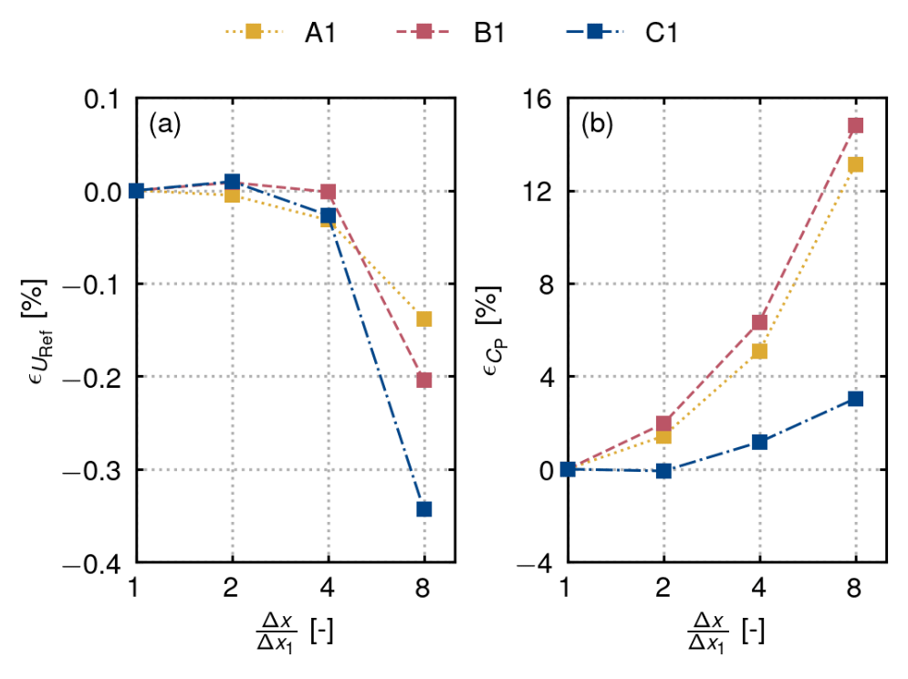
Figure 2 Change $\mathit{ϵ}=\frac{f-f_{\mathrm{1}}}{f_{\mathrm{1}}}$ in the variable f relative to the solution on the finest grid f₁ when increasing the cell side length Δx for the three considered domain types. (a) U_Ref and (b) C_P.

The impact of the domain size on the results has been studied in a previous work. For a turbine located on a hill, increasing the cross-sectional area of the computational domain by a factor of 8 results in a change in the disk-averaged velocity of less than 0.1 % for a fixed C_T (Zengler et al., 2024).

3 Results

The results are organized by first presenting undisturbed velocity profiles and selected flow fields at the respective turbine locations, then the obtained $C_{\mathrm{P}}-\mathit{\lambda }-\mathit{\theta }$ surfaces at these locations, analyzing the differences in C_P,max, λ_opt, and θ_opt. The controller constant k is set using the values of C_P,max and λ_opt obtained at the flat location (A0). Next, power curve calculations are performed at all three turbine positions for this controller, and control-relevant quantities and resulting flow fields are presented.

3.1 Freestream velocity and turbulence intensity profiles at the rotor position and flow fields

In Fig. 3, the undisturbed velocity profiles and turbulence intensity profiles at all considered turbine positions are shown. For all cases, the inflow profiles are identical to the profiles in flat terrain (A0/A1), corresponding to a neutral inflow at z₀=0.001 m as described by Eq. (12). Only for C2 are the inflow profiles different due to the higher surface roughness of z₀=0.1 m.

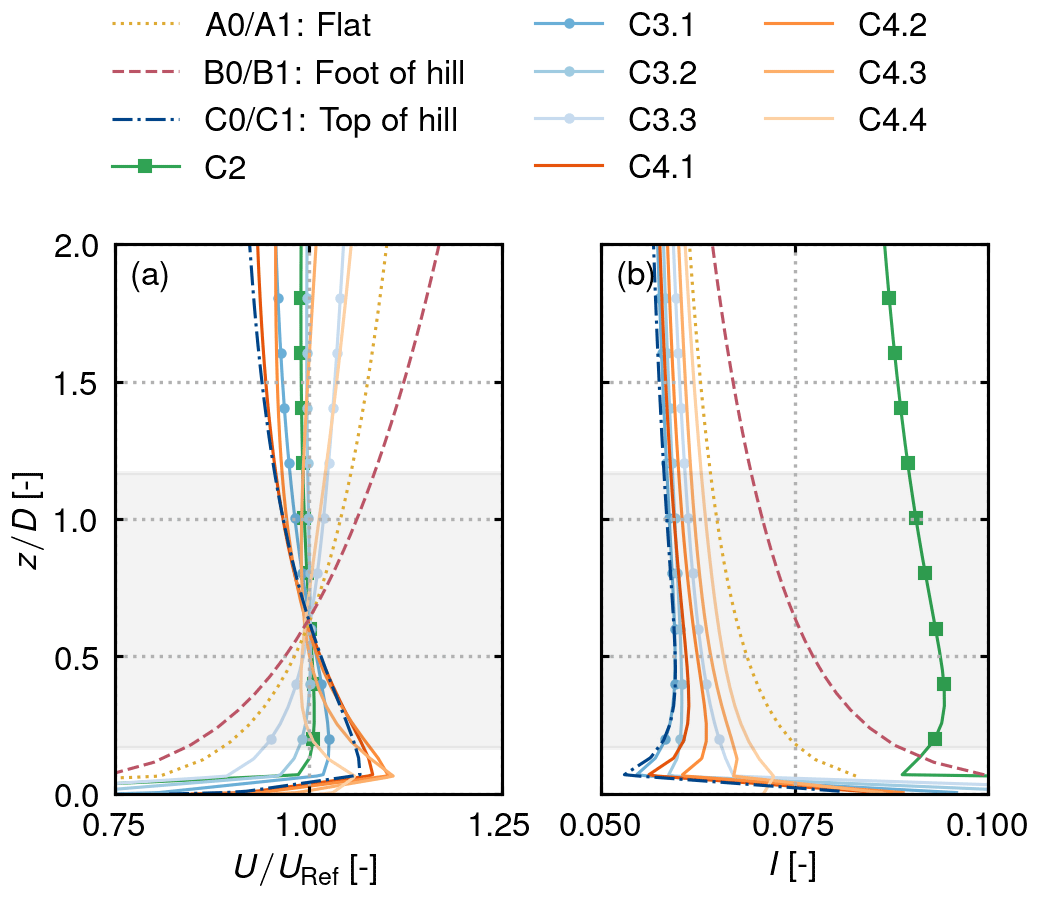
Figure 3 Undisturbed normalized velocity profiles U at the rotor position for all considered cases in (a) and turbulence intensity I in (b). Grey areas indicate the rotor position. In all cases, the inflow profiles of the simulations are identical to the flat-terrain profile, except for case C2, which has a higher surface roughness.

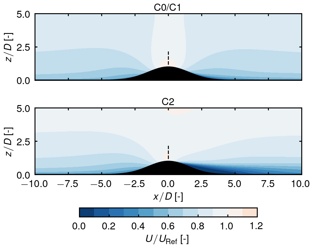
Figure 4 Undisturbed normalized flow fields (a) for cases of low roughness (C0/C1) and (b) the case of high roughness (C2). The dashed lines indicate the turbine position.

In flat terrain, the rotor-averaged turbulence intensity is 6.76 %. At the foot of the hill, the shear of the velocity profile is slightly higher than in flat terrain, and the turbulence intensity is also higher at 7.54 %. On top of the hill (C0/C1), negative shear due to the hill-induced speed-up close to the surface occurs, and the turbulence intensity is only 5.90 %. The cases C3.X–C4.X are mostly enclosed by the flat-terrain profiles and the highest-hill (C0/C1) profiles. With decreasing height, the profiles generally converge towards flat terrain. The hills of C4.X are steeper than the hills of C3.X, leading to a stronger speed-up close to the ground and higher levels of turbulence intensity. The case C2 shows very little shear over the rotor area and the highest levels of turbulence intensity of 9.25 %. The different shear profiles result in different distributions of kinetic energy across the rotor area, but this bias is accounted for by calculating the rotor-equivalent wind speed (Eq. 10) as a reference wind speed. Since turbulence intensity also affects turbine power performance, we assess the bias in the simulation results introduced by the different levels of turbulence intensity at the different turbine positions. The impact of turbulence intensity I on power can be estimated as (Elliot and Cadogan, 1990)

$$\begin{array}{}\text{(13)}& P\left(I\right)=P_{I=\mathrm{0}}\left(\mathrm{1}+\mathrm{3}{I}^{\mathrm{2}}\right).\end{array}$$

Based on the rotor-average of the turbulence intensity, it is expected that when neglecting any other effects, such as streamwise flow development, the power and also the power coefficient at the foot of the hill are approximately 0.33 % higher than in flat terrain at the same undisturbed wind speed and approximately 0.32 % lower on top of the hill for the lowest case of turbulence intensity. In the case of C2, we expect an impact of 1.18 %.

In Fig. 4, the undisturbed flow fields for representative cases at low roughness and high roughness are visualized. Behind the hill with high roughness, a separation region is clearly visible, whereas at low roughness, the flow remains attached to the surface. Notably, as mentioned before, the inflow fields are also slightly different.

3.2 $C_{\mathrm{P}}-\mathit{\lambda }-\mathit{\theta }$ surfaces

Figure 5 shows C_P as a function of the blade pitch angle and the tip-speed ratio for cases A0, B0, and C0. The surfaces are obtained on a coarse grid with Δλ=1 and Δθ= 1°, and the maxima are found by a nested grid search, where, based on the discrete maximum on the coarse grid, a finer region is defined. In this finer region, a surface with spacing Δλ= 0.1 and Δθ= 0.1° is simulated, and based on the obtained maximum within this region, an even finder grid with Δλ= 0.02 and Δθ= 0.02 is simulated. The final maxima are, in all cases, within the finest regions and not on their boundaries, ensuring that the optimum is actually in this region. On top of the hill, a sufficiently converged flow solution could not be reached for cases of λ = 10 and $\mathit{\theta }=-\mathrm{5}$, −4° due to the high loading on the flow. The combination of a high disk-based thrust coefficient (C_T>1) and a deceleration of the flow behind the ridge leads to oscillations in the solution, suggesting that it may be unsteady and not solvable with a steady-state RANS model.

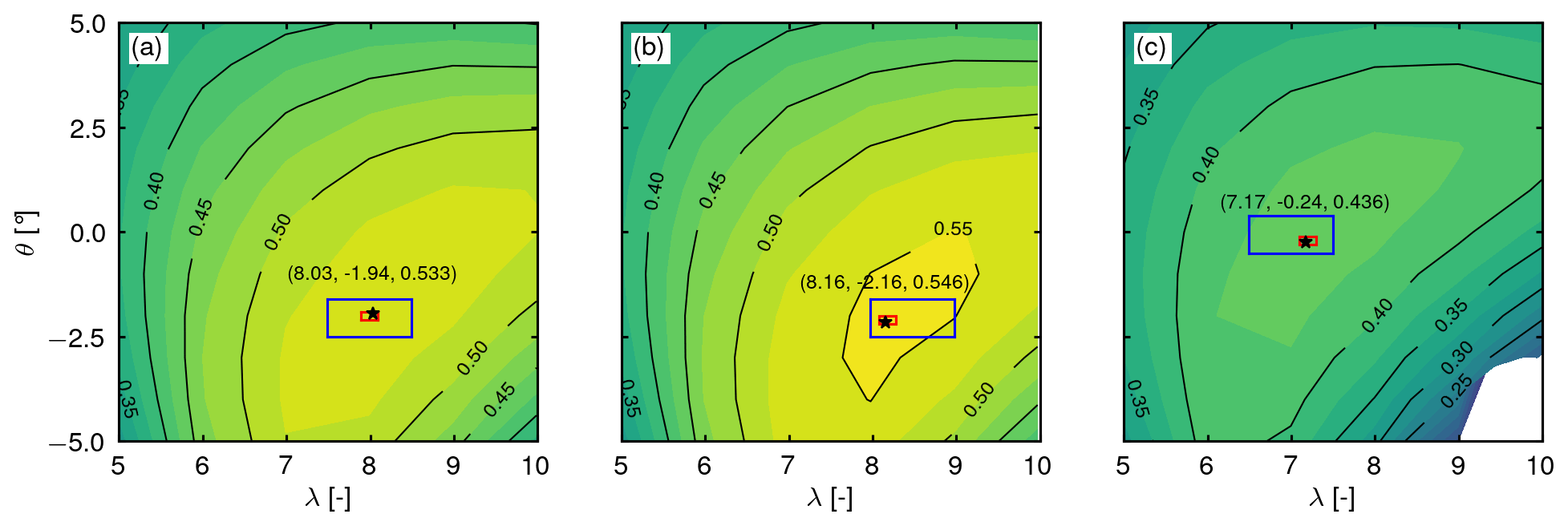
Figure 5 C_P surfaces obtained in (a) a flat domain A0, (b) on the foot of the hill B0, and (c) on top of the hill C0. Black stars indicate the point of optimal power performance. These discrete optima are found by a nested-grid search: the outer mesh grid has a spacing of Δλ=1 and Δθ=1°, within the blue square the grid spacing is Δλ=0.1 and Δθ=0.1°, and within the red square the spacing is Δλ=0.02 and Δθ=0.02°.

In flat terrain, the optimal C_P is 0.533 at a blade pitch angle of $\mathit{\theta }=-\mathrm{1.94}$° and a tip-speed ratio of 8.03. These values differ from the ones specified for the DTU 10 MW RWT (C_P≈0.474, θ=0.0, λ=7.5). The DTU 10 MW RWT was designed using an aeroelastic optimization tool with a blade element momentum model to represent the flow (Bak et al., 2013). In AD-CFD simulations, the induction is commonly underpredicted (Mikkelsen, 2004; Zengler et al., 2025a), leading to a higher performance compared to solely aeroelastic simulations, as shown by Hodgson et al. (2021) for the DTU 10 MW RWT. In combination with the region around maximum performance being comparably flat and the optimum being sensitive to modeling choices, this provides a likely explanation for the different optimal performance point we observe.

When the turbine is located at the foot of the hill, the maximum power performance increases by 2.46 %, accompanied by a decrease in optimal pitch (−2.16°) and an increase in the tip-speed ratio (8.16). At the top of the hill, the opposite is true. The maximum power coefficient decreases by 18.25 % together with an increase in pitch (−0.24°) and a decrease in the tip-speed ratio (7.17). Both on top of the hill and at its foot, the change in C_P is significantly greater than what one would expect due to the different levels of turbulence intensity at the position of the turbine, as discussed in the previous section.

The undisturbed velocity contours in Fig. 1 show that the flow accelerates behind the turbine located at the foot of the hill, while it decelerates behind the turbine at the hill top. In line with previous research (Revaz and Porté-Agel, 2024; Troldborg et al., 2022; Dar et al., 2023), deceleration results in a decrease in power performance, while acceleration results in an increase. The presented C_P surfaces indicate that there is no possibility of operating at the same optimal power coefficient as in the flat case when the turbine is operating on the hill, regardless of pitch and tip-speed ratio, because the power coefficient is limited by the flow development. However, this does not necessarily mean that placing a turbine on top of a hill leads to worse power performance in absolute numbers because wind speeds on top of hills are often higher. The actual benefit one can expect by placing a wind turbine on a hill is discussed in Sect. 4.3.

3.3 Simulations with active controller

The pitch and torque controllers are tuned based on the steady-state optimal performance in flat terrain (A0), and the resulting control constants are listed in Table 1. Simulation results with the controller are presented in two steps. First, quantities characterizing performance, such as power, C_P, and λ, are presented; second, the resulting flow fields around the turbine are shown.

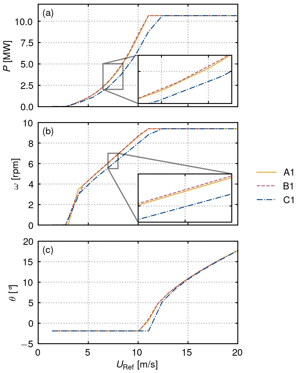
Figure 6 Power curves obtained with the controller in flat terrain (A1), ahead of the hill (B1), and on top of the hill (C1) with the power in (a), the respective rotor speed in (b), and the blade pitch in (c).

With the calibrated controller, the power curves are obtained by varying the friction velocity u_* in Eq. (12). The results for flat terrain, ahead of the hill, and on top of the hill are shown in Fig. 6, with the power shown in panel (a). The turbine on top of the hill produces significantly less energy below rated wind speed than the one in flat terrain for the same undisturbed wind speed at the rotor, while the one at the hill's foot produces slightly more energy for the same undisturbed rotor wind speed. Note that although the wind speed changes, Reynolds similarity leads to the development of similar flow features independent of the wind speed (van der Laan et al., 2020), which is why the induction below rated wind speed is unaltered by the inflow velocity. Above rated conditions, all turbines produce the same power as a consequence of the pitch controller aiming to maintain a certain rotor speed independently of the maximum available power in the flow. The corresponding rotor speed, shown in Fig. 6b, exhibits the same behavior as the power, being slightly higher ahead of the hill and significantly lower at the hilltop. Inspection of the blade pitch in Fig. 6c shows that, below rated conditions, the pitch is identical for all cases, settling at −1.94°. When reaching rated conditions, the controller of the turbine ahead of the hill starts to pitch at lower wind speeds than in flat terrain, whereas the opposite is true for the turbine on the hilltop. This can be attributed to the different rotor speeds, which serve as an input signal for the pitch controller. Overall, the reported trends are in agreement with the results by Troldborg et al. (2022).

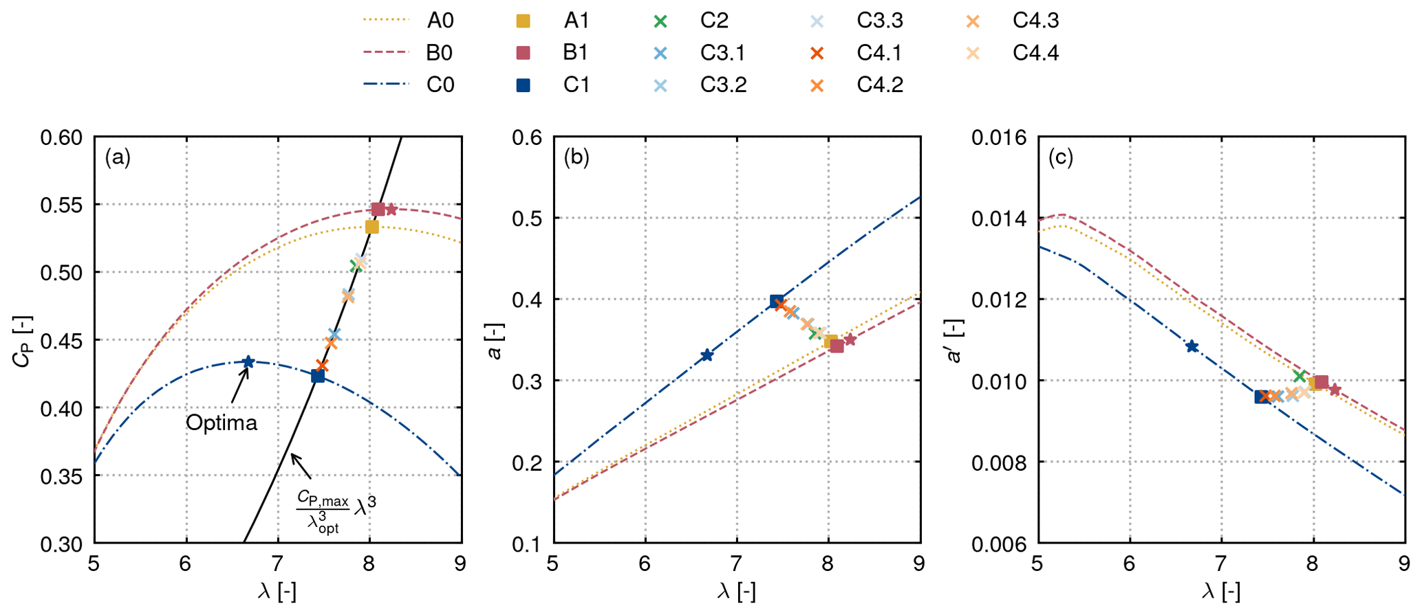
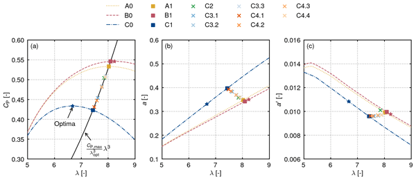
Figure 7 Simulation results for the controlled turbine placed at the different positions: (a) C_P−λ curves with control curve in solid black, steady-state operational points below rated wind speed marked as crosses, and discrete maximum C_P marked by stars; (b) induction curves and operational points with $a=\mathrm{1}-u_{\mathrm{R}}/U_{\mathrm{Ref}}$, where u_R is the kinetic energy mean over the rotor calculated like U_Ref in Eq. (10); and (c) tangential induction a^′ evaluated as azimuthal mean at r=0.75R.

Turning towards the non-dimensional quantities characterizing turbine operation in region 2, Fig. 7a shows the C_P−λ curves of A0, B0, and C0 at $\mathit{\theta }=-\mathrm{1.94}$°, including the points where the torque controller settles in region 2 during the power curve calculation for all considered simulations. Regardless of the turbine position, the controller settles at the intersections of the control curve given by Eq. (7) and the respective performance curves as shown for cases A0/A1, B0/B1, and C0/C1. Specifically for case C1, it becomes apparent that this intersection does not necessarily represent the point of maximum power performance. In numbers, at the foot of the hill, the C_P at which the controller settles is 2.40 % higher than in flat terrain, while it is 20.63 % lower on top of the hill. If the torque constant were tuned to match the optimal tip-speed ratio in both cases, the gain ahead of the hill would be around 2.45 %, while on top of the hill, the loss would reduce to 18.67 %. Adjusting also the blade pitch would further improve the results, as shown in Fig. 5.

Figure 7b shows the axial induction as a function of λ. At the foot of the hill, it is always lower than in flat terrain, while on top of the hill, it is always higher, corresponding to a higher and lower C_P, respectively. At the top of the hill, the optimal tip-speed ratio would be approximately 6.7, resulting in a lower induction relative to the flat case. However, the controller settles at a tip speed ratio of 7.4 with an increased induction relative to the flat case. There is a general trend that for the controlled turbine, the induction decreases with an increasing tip-speed ratio.

In Fig. 7c, the azimuthally averaged tangential induction $a^{\prime }=u_{R,t}/\left(\mathit{\omega }r\right)$ evaluated at 0.75 R is presented. The $a^{\prime }-\mathit{\lambda }$ curves show an opposite trend to the a−λ curves. The tangential induction generally decreases with an increasing tip-speed ratio; however, for a given tip-speed ratio, it is always lower at the top of the hill and higher ahead of the hill, which is opposite to the trend followed by the axial induction. In comparison to the axial induction, the tangential induction of the controlled cases seems to stay rather constant during operation at the three different locations. Only a small trend can be observed: ahead of the hill, the tangential induction increases, while it decreases on top of the hill. An outlier is case C2, the one with the higher surface roughness compared to case C1, showing a higher tangential induction than all other cases. In Sect. 4.1, it is discussed whether tangential induction is expected to stay constant during torque control. There, the radial distributions of axial and tangential induction are also shown.

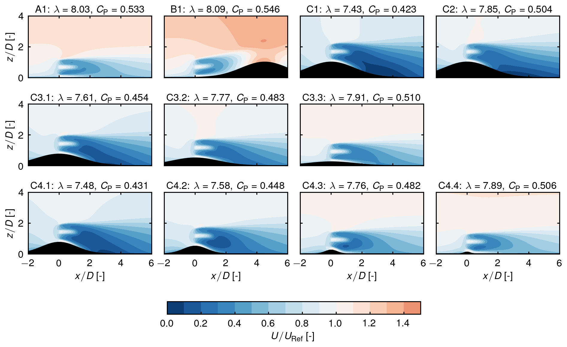
Figure 8 Flow fields developing around the turbine operating with an active controller for the investigated cases.

After presenting performance quantities only, we will now extend the results by also presenting the respective flow fields for all cases. Figure 8 shows velocity contours in the x–z plane through the rotor center. Velocities are normalized by the undisturbed velocity at the turbine position. Note that in all cases, the x coordinate is relative to the position of the rotor.

Case C1 in Fig. 8 shows that the flow speed is lower everywhere around the turbine, while for case B1, one can see that the hill behind the turbine accelerates the flow around the turbine. Comparing cases C1 and C2, the velocity deficit in the wake is lower in the latter case. It has already been noted by Revaz and Porté-Agel (2024) that there is a strong negative correlation between the maximum velocity deficit in the wake and the respective power performance, although there are exceptions specifically for cases where flow separation occurs. A comparison of the second and third rows of Fig. 8 shows that at a given hill height, the power performance is higher for the wider hill or the lower maximum slope, respectively, which is in agreement with Revaz and Porté-Agel (2024) and Zengler et al. (2024). Comparing the panel of C3.3 with the panel of A1 already indicates how an increasing widening of the hill leads to a flow field around the turbine converging towards a field close to flat conditions.

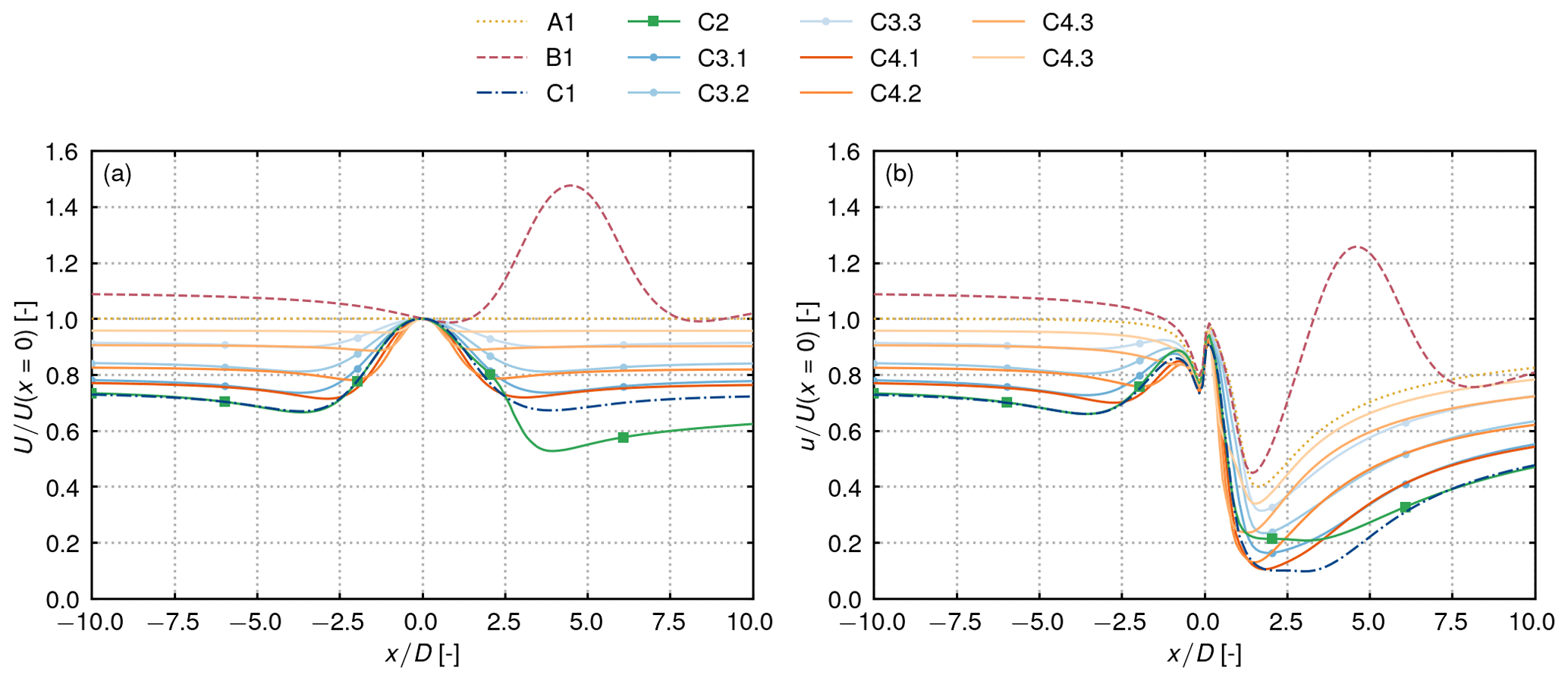
Figure 9 Velocity at hub height (terrain following) without turbine operating in (a) and with turbine operating in (b), with the turbine being located at x=0.

Figure 9 shows the undisturbed and disturbed velocities at constant height above ground (hub height). The figure reveals several noteworthy characteristics. First, it is observed that the undisturbed flow does not accelerate at the turbine position ahead of the hill but rather slightly behind it. This indicates that predicting power performance bias solely by evaluating acceleration at the turbine position is insufficient and that the flow field downstream also needs to be considered, as previously mentioned (Zengler et al., 2024). A comparison of cases C1 (low roughness) and C2 (high roughness) shows a nearly identical development of the undisturbed hub height velocity ahead of the hill, whereas the deficit behind the hill is markedly deeper in C2. When the turbine is operating, the opposite behavior is observed. This indicates a non-linear interaction between turbine, flow, and terrain. Comparing cases with the same hill height but different widths (C3.1–C3.3 and C4.1–C4.3) shows that, at a given hill height, the flow field differs only near the turbine, with stronger acceleration and deceleration for the narrower hills. In all cases, there is a speed-up directly at the turbine position when the turbine is operating (also visible in Fig. 8). This is a consequence of the missing nacelle, which leads to a channeling of the flow through the rotor center.

4 Discussion

The previous section showed that the power performance is markedly affected when a flat-terrain-designed turbine operates under complex-terrain conditions. This is primarily a consequence of the flow physics, as seen in Fig. 5. Additionally, the controller leads to suboptimal performance in these situations, as seen in Fig. 7a.

Now, we characterize the behavior of the torque and pitch controllers. Furthermore, we investigate how much the turbine's actual power output on the hilltop differs from what would be expected from the speed-up alone. Lastly, the limitations of the present study are discussed.

4.1 Role of torque controller

Figure 7a shows that the torque controller follows its prescribed control curve as expected, even when the surrounding flow field changes to conditions the controller was not calibrated for. On the one side, this is not surprising because, as shown in Eq. (7), the torque controller effectively enforces

$$\begin{array}{}\text{(14)}& {\displaystyle \frac{C_{\mathrm{P},\max }}{{\mathit{\lambda }}_{\mathrm{opt}}^{\mathrm{3}}}}={\displaystyle \frac{C_{\mathrm{P}}}{{\mathit{\lambda }}^{\mathrm{3}}}}\end{array}$$

for any operational state, with the left-hand side being constant and calibrated, for example, for flat terrain in our case. On the other hand, this relation does not directly yield insights into how a and the local a^′ change due to complex terrain, which is analyzed in the following.

4.1.1 Impact on axial induction and performance coefficients

We formulate the torque control strategy based on the velocity at the disk during operation. For this purpose, we introduce the operational power coefficient, thrust coefficient, and tip-speed ratio as follows:

$$\begin{array}{}\text{(15)}& {\displaystyle }{C}_{\mathrm{P}}^{*}={\displaystyle \frac{P}{\frac{\mathrm{1}}{\mathrm{2}}\mathit{\rho }{u}_R^{\mathrm{3}}A}}=C_{\mathrm{P}}{\left({\displaystyle \frac{U_{\mathrm{Ref}}}{u_{\mathrm{R}}}}\right)}^{\mathrm{3}},\text{(16)}& {\displaystyle }{C}_{\mathrm{T}}^{*}={\displaystyle \frac{T}{\frac{\mathrm{1}}{\mathrm{2}}\mathit{\rho }{u}_R^{\mathrm{2}}A}}=C_{\mathrm{T}}{\left({\displaystyle \frac{U_{\mathrm{Ref}}}{u_{\mathrm{R}}}}\right)}^{\mathrm{2}},\text{(17)}& {\displaystyle }{\mathit{\lambda }}_{*}={\displaystyle \frac{\mathit{\omega }R}{u_{\mathrm{R}}}}=\mathit{\lambda }{\displaystyle \frac{U_{\mathrm{Ref}}}{u_{\mathrm{R}}}},\end{array}$$

where u_R is the flow in the turbine plane during operation, calculated using Eq. (10). The optimal power operation is then reformulated as

$$\begin{array}{}\text{(18)}& P_{max}={\displaystyle \frac{\mathrm{1}}{\mathrm{2}}}\mathit{\rho }\mathit{\pi }{R}^{\mathrm{2}}{C}_{\mathrm{P},\max }^{*}{u}_{\mathrm{R}}^{\mathrm{3}}=\underset{k}{\underbrace{{\displaystyle \frac{\mathrm{1}}{\mathrm{2}}}\mathit{\rho }\mathit{\pi }{R}^{\mathrm{5}}{\displaystyle \frac{C_{\mathrm{P},\max }^{*}}{{\mathit{\lambda }}_{*\mathrm{opt}}^{\mathrm{3}}}}}}{\mathit{\omega }}^{\mathrm{3}},\end{array}$$

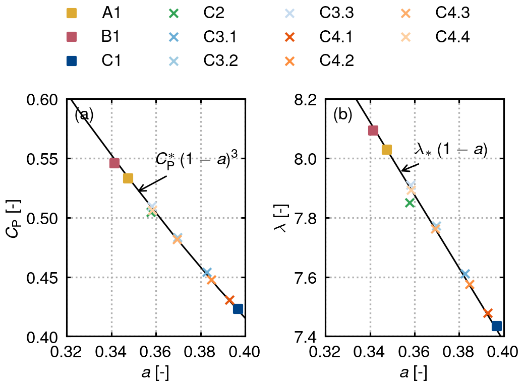
with the control constant k being the same as the one defined in Eq. (3) because u_D and U_Ref cancel out in both equations, respectively. This shows that optimal control actually enforces an equilibrium between power and the velocity in the turbine plane during operation, independently of the freestream velocity. This makes intuitive sense because eventually the forces and moments on the turbine blades purely depend on what the local flow is at the disk. In fact, the only quantity that a torque controller keeps constant is the ratio between torque and rotor speed squared, regardless of what velocity is used as reference velocity, as seen in Eq. (5). Because rotor speed and disk velocity are related by a constant during torque control in order to keep the local flow angles constant, an equilibrium between power and disk velocity during operation is also achieved (Zengler et al., 2025b). Thus, a turbine calibrated for a certain operational point keeps $C_{\mathrm{P}}^{*}$ constant and not C_P. We find for all cases $C_{\mathrm{P}}^{*}\approx \mathrm{1.92}$, $C_{\mathrm{T}}^{*}\approx \mathrm{2.27}$ and ${\mathit{\lambda }}_{*}\approx \mathrm{12.31}$.

The introduction of certain non-dimensional quantities hides the actual physics. The relation between C_T and a changes in terrain but not the relation between the local blade forces and velocities. To circumvent this problem, one could either use quantities for non-dimensionalization that do not change, such as u_R in our case, or work exclusively in dimensional form.

Returning to torque control, for the optimal thrust, it follows that

$$\begin{array}{}\text{(19)}& T_{\mathrm{opt}}={\displaystyle \frac{\mathrm{1}}{\mathrm{2}}}\mathit{\rho }\mathit{\pi }{R}^{\mathrm{2}}{C}_{T\mathrm{opt}}^{*}{u}_{\mathrm{R}}^{\mathrm{2}}=\underset{\mathrm{constant}}{\underbrace{{\displaystyle \frac{\mathrm{1}}{\mathrm{2}}}\mathit{\rho }\mathit{\pi }{R}^{\mathrm{4}}{\displaystyle \frac{C_{T\mathrm{opt}}^{*}}{{\mathit{\lambda }}_{*\mathrm{opt}}^{\mathrm{2}}}}}}{\mathit{\omega }}^{\mathrm{2}},\end{array}$$

from which the following can be deduced:

$$\begin{array}{}\text{(20)}& {\displaystyle \frac{C_{\mathrm{T}}}{{\mathit{\lambda }}^{\mathrm{2}}}}={\displaystyle \frac{C_{\mathrm{T}}^{*}}{{\mathit{\lambda }}_{*}^{\mathrm{2}}}}=\mathrm{constant}.\end{array}$$

How do these considerations now affect a, a^′, C_P, and C_T during torque control? Based on Eqs. (15)–(17), the following relations are obtained:

$$\begin{array}{}\text{(21)}& {\displaystyle }{C}_{\mathrm{P}}=C_{\mathrm{P}}^{*}{\left(\mathrm{1}-a\right)}^{\mathrm{3}},\text{(22)}& {\displaystyle }{C}_{\mathrm{T}}=C_T^{*}{\left(\mathrm{1}-a\right)}^{\mathrm{2}},\text{(23)}& {\displaystyle }\mathit{\lambda }={\mathit{\lambda }}_{*}\left(\mathrm{1}-a\right).\end{array}$$

Figure 10 shows Eqs. (21) and (23) alongside the simulation results and reveals that the turbine indeed always operates on these curves. At this point, it is worth taking a look at control strategies, which set blade forces based on u_R and $C_{\mathrm{T}}^{*}$ (van der Laan et al., 2014; Meyers and Meneveau, 2010; Calaf et al., 2010). The current findings show that classical torque control is equivalent to these strategies, keeping $C_{\mathrm{T}}^{*}$ and $C_{\mathrm{P}}^{*}$ constant, rather than C_T and C_P, which has also been shown previously (Zengler et al., 2025b). This is an important finding, as it shows that using disk-based quantities for a simplified control yields identical results to k−ω² control in region 2 of the power curve, irrespectively of the development of the flow field. It must be noted though that this does not apply to region 3, where the modified induction in non-uniform flows can lead to different pitch signals and consequently differing power performance.

Figure 10 Power coefficient in (a) and tip-speed ratio in (b) as a function of the induction in flat terrain, ahead of the hill and on top of it together with Eqs. (21) and (23) using $C_{\mathrm{P}}^{*}=\mathrm{1.92}$ and ${\mathit{\lambda }}_{*}=\mathrm{12.31}$.

4.1.2 Impact on tangential induction

In the following, the reason why the tangential induction a^′, as shown in Fig. 7c, is only vaguely sensitive to terrain effects is explained. In Appendix A, it is shown that by disregarding drag, the local tangential induction can be calculated as

$$\begin{array}{}\text{(24)}& a^{\prime }\left(\mathit{\mu }\right)={\displaystyle \frac{\mathrm{1}}{\mathrm{2}}}\left(-\mathrm{1}+\sqrt{\mathrm{1}+{\displaystyle \frac{C_{\mathrm{t}}\left(\mathit{\mu }\right)}{{\mathit{\lambda }}^{\mathrm{2}}{\mathit{\mu }}^{\mathrm{2}}}}}\right),\end{array}$$

with the non-dimensional radial coordinate $\mathit{\mu }=r/R$ and the local thrust coefficient C_t. From this equation, it is evident that a^′ only depends on the local blade forces and rotor speed. The reference velocity used for normalization of λ and C_t can be omitted from the equation because C_t is normalized by $U_{\mathrm{Ref}}^{\mathrm{2}}$ and λ by U_Ref, so when dividing C_t by λ², U_Ref cancels out. It was shown in Eq. (20) that the ratio $\frac{C_{\mathrm{T}}}{{\mathit{\lambda }}^{\mathrm{2}}}$ is constant for a torque controller. Based on this, it can now be argued that the local version of that ratio $\frac{C_{\mathrm{t}}\left(\mathit{\mu }\right)}{{\mathit{\lambda }}^{\mathrm{2}}}$ should be constant as well, as long as changes in the flow state due to terrain are uniform over the disk. This explains why a^′ is independent of the effects of complex terrain in region 2, although rotor speed and thrust change; it is simply a consequence of the torque control. In Fig. 11a and b, the local axial and tangential inductions are shown. While the axial induction varies significantly between the presented cases, the tangential induction is nearly identical in all cases. Deviations between the cases are only visible close to the root. A possible explanation for this is that in this region drag plays a significant role, also affecting the tangential induction.

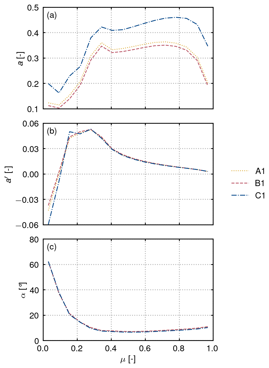
Figure 11 Azimuthally averaged axial induction (a), tangential induction (b), and angle of attack α (c) shown as a function of non-dimensional radial position $\mathit{\mu }=r/R$.

Lastly, Fig. 11c shows the local angle of attack α. Since the local tip-speed ratio λ_* and flow angles remain constant, it does not come as a surprise that the angles of attack do not change during torque control, supporting the analysis in the previous section.

In summary, a torque controller enforces $C_{\mathrm{P}}^{*}$, $C_{\mathrm{T}}^{*}$, and λ_* to stay constant. A consequence is that a^′ is also constant, which only depends on the local forces and flow. Because of the changing optimal inflow angles in complex terrain, a torque controller tuned for flat terrain cannot operate optimally with this strategy.

4.1.3 Optimal performance

We briefly discuss how a controller would need to operate to always track optimal performance. From Eq. (23), one can see that the rotor speed at a given reference velocity (λ) decreases with a decreasing disk velocity (an increasing induction). In Fig. 7b, the optimal performance on top of the hill would be reached by reducing the induction and the tip-speed ratio. From a local perspective, this results in higher axial velocities and lower relative tangential velocities. As a consequence, the local flow angle and angle of attack increase when the pitch is not adjusted. However, as suggested by Fig. 5, the pitch should also be modified to track optimal performance, which would eventually change the angle of attack.

Ahead of the hill, when the background flow accelerates, the opposite is the case; to track optimal performance, the angle of attack would need to decrease. This observation is also in agreement with previous findings based on momentum theory (Zengler et al., 2025a, see also Eq. B5), which show that in a decelerating flow, the optimal performance would be reached at a lower induction, while in an accelerating flow, it would be reached at a higher induction. Without modification of the torque constant, a torque controller would therefore always operate below optimum in accelerating flow fields because it effectively keeps flow angles constant instead of adjusting them to the flow conditions. Since blades are often designed to achieve the best two-dimensional polar lift-to-drag ratios at the angles of attack corresponding to region 2 operation, torque control ensures that the airfoil sections perform well from a two-dimensional perspective. The reason for suboptimal power performance is the changed (axial) induction response in accelerating flows.

A way of approaching this problem of suboptimal power performance outside the flat operating conditions would be to include control algorithms, which slowly modify the torque constant (and pitch) over time to reach optimal performance (see, for example, extremum seeking control, Creaby et al., 2009). However, as indicated by Fig. 7b, the total gain in performance is rather low on a given curve. Also, the gradient $\frac{\partial C_{\mathrm{P}}}{\partial \mathit{\lambda }}$ might not be very strong. In combination with varying atmospheric conditions, which are not part of this study, and also seasonal variations in the terrain surface, optimization of the torque constant might be difficult and the expected gain possibly small, if not even negligible.

4.2 Role of the pitch controller in region 2

The pitch controller tracks the difference between the actual and rated rotor speed. In region 3 of the power curve, this leads to the observed behavior that even in a non-uniform background flow, the same rated power is reached in the different cases. In region 2, the pitch controller remains inactive, although Fig. 5 suggests that performance could be increased by adjusting the pitch. The reason for this is the implementation of the pitch controller as a PI controller. Below the rated wind speed, or rather the rated rotor speed, the difference between actual and rated rotor speed is negative, resulting in a negative pitch signal saturating at the minimum pitch independently of the flow state. Similarly to the torque controller, one could imagine an algorithm that modifies the minimum pitch seeking maximum power performance in region 2 of the power curve. However, in practice, it might again be difficult because of the small differences between optimal and actual pitch.

4.3 Speed-up factors

A common way to account for the effect of complex terrain is to use speed-up factors. Because power scales with the wind speed cubed in the flat-terrain case, the effect of terrain on the power of a turbine is usually estimated as

$$\begin{array}{}\text{(25)}& P_{\mathrm{hill}}\approx P_{\mathrm{flat}}(\mathrm{1}+\mathrm{\Delta }U{)}^{\mathrm{3}},\end{array}$$

with $\mathrm{\Delta }U=(U_{\mathrm{Ref},\mathrm{hill}}-U_{\mathrm{Ref},\mathrm{flat}})/U_{\mathrm{Ref},\mathrm{flat}}$ being a non-dimensional velocity speed-up factor. This estimate is only accurate as long as the actual power coefficient of the turbine is the same as that in the flat-terrain case. However, as shown above, placing the turbine on a hill reduces the power coefficient due to the streamwise evolution of the downstream flow. This raises the question of what is actually the maximum performance that can be reached by placing wind turbines on elevated spots, such as hills.

To address this question, we analyze all simulations with the turbine located on top of the hill using the model by Zengler et al. (2025a). The model can predict the maximum power coefficient C_P,max as a function of the speed-up, ΔU, by assuming that the maximum deceleration behind the hill is comparable to the speed-up ahead of it and that the speed-up region is smaller than the region in which the wake pressure equalizes with the surrounding pressure. This is outlined in Appendix B in more detail. Because this model yields identical results to momentum theory for ΔU=0, the scaling of the power on a hill can be estimated to be

$$\begin{array}{}\text{(26)}& {\displaystyle }{P}_{\mathrm{hill}}=P_{\mathrm{flat}}{\displaystyle \frac{C_{\mathrm{P},\max }\left(\mathrm{\Delta }U\right)}{C_{\mathrm{P},\max }(\mathrm{\Delta }U=\mathrm{0})}}(\mathrm{1}+\mathrm{\Delta }U{)}^{\mathrm{3}},\text{(27)}& {\displaystyle }=P_{\mathrm{flat}}{\displaystyle \frac{C_{\mathrm{P},\max }\left(\mathrm{\Delta }U\right)}{\mathrm{16}/\mathrm{27}}}(\mathrm{1}+\mathrm{\Delta }U{)}^{\mathrm{3}},\text{(28)}& {\displaystyle }\approx P_{\mathrm{flat}}(\mathrm{1}+\mathrm{\Delta }U{)}^{\mathrm{1.5}},\end{array}$$

with C_P,max calculated from Eqs. (B4) and (B6) and the third line being an approximation based on visual inspection of the resulting curves. This estimate requires that the flow recovers to the flat-terrain state directly behind the turbine and can therefore be interpreted as a lower bound to the possible maximum power performance. To investigate the power increase on top of the hill in the presented simulations, Fig. 12 compares the simulated power increase with the traditional cubic trend (Eq. 25), the lower bound from Eq. (27) and its approximation Eq. (28), as well as a quadratic scaling for reference. It is important to keep in mind that the simulation results also include a controller; thus, the actual maximum available power is expected to be around 1 % higher, as shown in Fig. 7a.

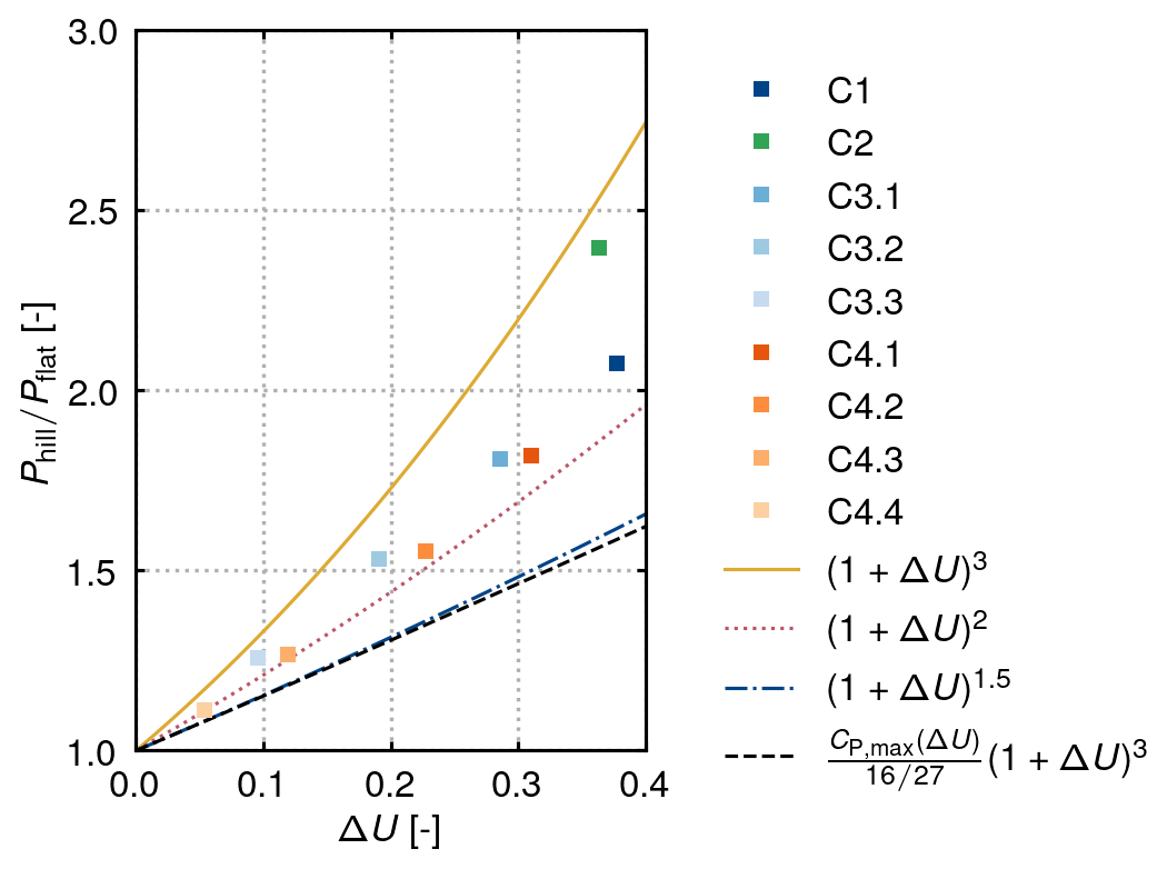
Figure 12 Expected and actual power at the top of the hill for different speed-up factors. The turbines were simulated, including a controller, so the potential maximum power performance would be around 1 % higher.

As expected, the actual power increase on top of the hill does not follow a cubic trend but is lower in all cases. When the flow separates behind the hill, as is the case for z₀=0.1 m (C2), and the velocity immediately behind the turbine does not decelerate so strongly, the power is closer to the cubic relationship. The same conclusions can be made comparing simulations C3.1–C3.3 with C4.1–C4.4. When the width does not change, the deceleration behind the turbine is weaker, and the respective power performance is higher. Reducing both width and height results in a more local speed-up followed by a strong deceleration. None of the presented cases seems to scale according to Eq. (27) but rather mostly show a scaling close to quadratic. Only for very small speed-ups does the scaling seem to approach our theoretical predictions. As outlined previously, this can be explained through the assumptions made for deriving Eq. (27), which requires a very local speed-up with immediate wake recovery. These observations suggest that if terrain and flow features in the vicinity of the turbine are more similar to flat-terrain features, such as a very long hill or a separation bubble that delays deceleration, the maximum power coefficients are also similar, leading to a more cubic scaling of power. If this is not the case, and flow and terrain features vary on similar length scales to those of the turbine, a stronger influence on the power coefficient can be expected.

The above analysis shows that, although higher wind speeds at a hilltop lead to increased power output, flow deceleration reduces the achievable gain compared to that predicted by the classical cubic scaling. In cases where turbines are located in smaller local freestream speed-up regions, the scaling is closer to quadratic and may theoretically be even lower.

4.4 Limitations

Although this work deals with complex terrain, the studied case of an AD on a quasi-two-dimensional Gaussian hill remains a significant simplification. The undisturbed flow field is quasi-two-dimensional and varies only in the vertical and streamwise direction. Furthermore, the effect of atmospheric stability was not included. It remains a subject for future studies how a three-dimensional, unsteady flow would interact with the wind turbine and to what extent the result that optimal induction decreases in a decelerating flow and increases in an accelerating flow also holds there. In this light, it would also be important to apply a more sophisticated turbine model, such as an actuator line model or a fully resolved turbine model, which leads to a more accurate representation of the local blade flow. This study focused on k−ω² control only; however other approaches to maximizing power performance in region 2, such as tip-speed ratio tracking (Abbas et al., 2022), exist as well, and it would be of interest how these would perform in complex-terrain conditions.

5 Conclusions

Wind turbine performance in complex terrain is affected by a streamwise non-uniform flow field, resulting in changing limits of maximal energy extraction and by the control algorithm, not capable of adjusting properly to the physics caused by the modified flow conditions. It was shown that a torque controller keeps thrust and power coefficient based on the disturbed flow field constant, which do not necessarily correspond to the point of operation, which yields maximum power performance in non-uniform flow fields. The present results suggest that a torque-based control calibrated for flat terrain would lead to suboptimal power performance in complex terrain because the optimal local flow angles change, whereas a torque controller keeps them constant. However, this effect seems to be rather small. It remains to be investigated whether it is practically beneficial to include additional knowledge about the flow field in the control strategy, as well as adjusting the torque constant and pitch. It was shown that placing turbines in elevated regions with higher wind speeds improves power production. However, the degradation of the power coefficient leads to a reduced power output, not scaling with the speed-up over the hill cubed. The observed scaling in the simulations was closer to a quadratic trend, while theoretical considerations suggest a lower limit of the scaling close to the power of 1.5.

Appendix A: The effect of flow acceleration on the tangential induction

The simulation results show that the tangential induction is barely affected by the acceleration of the background flow, and major differences between the simulations can only be observed close to the root. At the root, the energy conversion process is different compared to the blade tips because structural constraints require thick airfoils with a low lift-to-drag ratio, resulting in a flow that is significantly influenced by the drag of the airfoil. With this knowledge in mind, we now seek to investigate why the tangential induction is rather independent of flow acceleration in the outer region of the blade.

A control volume analysis of the conservation of angular momentum yields (Hansen, 2015)

$$\begin{array}{}\text{(A1)}& \mathrm{d}Q=r{u}_t^{+}\mathrm{d}\dot{m}=\mathrm{4}\mathit{\pi }\mathit{\rho }{R}^{\mathrm{2}}{\mathit{\mu }}^{\mathrm{3}}\mathit{\lambda }{U}_{\mathrm{Ref}}^{\mathrm{2}}(\mathrm{1}-a)a^{\prime }\mathrm{d}r,\end{array}$$

with $u_t^{+}$ being the tangential velocity in the wake, which relates to the tangential induction as $a^{\prime }=u_t^{+}/\left(\mathrm{2}\mathit{\omega }r\right)$. Further, we used d$\dot{m}=U_{\mathrm{Ref}}(\mathrm{1}-a)\mathrm{2}\mathit{\pi }r\mathrm{d}r$ for the mass flux. Note that U_Ref(1−a) only describes the velocity in the rotor plane, independently of what caused this velocity. Shifting the view towards the blade, the angular momentum can be calculated as

$$\begin{array}{}\text{(A2)}& \mathrm{d}Q=f_{\mathrm{t}}{N}_{\mathrm{B}}r\mathrm{d}r,\end{array}$$

with the tangential force per span length f_t and the number of blades N_B. When taking a look at the force and flow vectors at each blade section, we now consciously ignore the drag of the airfoil, yielding for the flow angle ϕ

$$\begin{array}{}\text{(A3)}& \tan \mathit{\varphi }={\displaystyle \frac{U_{\mathrm{Ref}}(\mathrm{1}-a)}{\mathit{\omega }r(\mathrm{1}+a^{\prime })}}={\displaystyle \frac{f_{\mathrm{t}}}{f_{\mathrm{n}}}},\end{array}$$

with the blade normal force per span length f_n. For the local thrust coefficient, we obtain

$$\begin{array}{}\text{(A4)}& C_{\mathrm{t}}={\displaystyle \frac{\mathrm{d}T}{\frac{\mathrm{1}}{\mathrm{2}}\mathit{\rho }{U}_{\mathrm{Ref}}^{\mathrm{2}}\mathrm{d}A}}={\displaystyle \frac{\mathrm{d}T}{\mathit{\pi }\mathit{\rho }{U}_{\mathrm{Ref}}^{\mathrm{2}}r\mathrm{d}r}}={\displaystyle \frac{f_{\mathrm{n}}{N}_{\mathrm{B}}}{\mathit{\pi }\mathit{\rho }{U}_{\mathrm{Ref}}^{\mathrm{2}}r}}.\end{array}$$

Combining Eq. (A3) with Eq. (A4) yields for the tangential force

$$\begin{array}{}\text{(A5)}& f_{\mathrm{t}}={\displaystyle \frac{\mathrm{1}-a}{\mathrm{1}+a^{\prime }}}{\displaystyle \frac{\mathit{\pi }R\mathit{\rho }{U}_{\mathrm{Ref}}^{\mathrm{2}}{C}_{\mathrm{t}}}{\mathit{\lambda }{N}_{\mathrm{B}}}},\end{array}$$

and by combining this with Eqs. (A1) and (A2), we obtain

$$\begin{array}{}\text{(A6)}& a^{\prime }(\mathrm{1}+a^{\prime })={\displaystyle \frac{C_{\mathrm{t}}}{\mathrm{4}{\mathit{\lambda }}^{\mathrm{2}}{\mathit{\mu }}^{\mathrm{2}}}},\end{array}$$

which can be solved for the tangential induction yielding Eq. (24), showing that, indeed, in regions where lift dominates the flow, the tangential induction only depends on $\frac{C_{\mathrm{t}}}{{\mathit{\lambda }}^{\mathrm{2}}}$, which a torque controller keeps constant.

The same result can be obtained in a vortex-theory framework without the need for a control-volume analysis, which is briefly outlined below. For an actuator disk with azimuthal constant loading, the induced tangential velocity due to the bound vortex system of strength N_BΓ_B can be calculated from the definition of the circulation Γ.

The circulation is generally written as

$$\begin{array}{}\text{(A7)}& \mathrm{\Gamma }=\oint u_{s}ds,\end{array}$$

with u_s being the tangential velocity along the curve s. This yields for the bound vortex system

$$\begin{array}{}\text{(A8)}& N_{\mathrm{B}}{\mathrm{\Gamma }}_{\mathrm{B}}=\mathrm{2}\mathit{\pi }r{u}_{t,i}^{+},\end{array}$$

with $u_{t,i}^{+}$ being the mean induced velocity behind the disk. Ahead of the turbine, the mean induced velocity is $u_{t,i}^{-}=\mathrm{0}$, and therefore in the disk plane the induced velocity is

$$\begin{array}{}\text{(A9)}& u_{t,i}={\displaystyle \frac{\mathrm{1}}{\mathrm{2}}}\left(u_{t,i}^{-}+u_{t,i}^{+}\right)={\displaystyle \frac{N_{\mathrm{B}}{\mathrm{\Gamma }}_{\mathrm{B}}}{\mathrm{4}\mathit{\pi }r}}.\end{array}$$

Based on the Kutta–Joukowsky condition, the axial force per span length f_n is calculated from

$$\begin{array}{}\text{(A10)}& \left[\begin{array}{c}-f_{\mathrm{n}}\\ -f_{\mathrm{r}}\\ -f_{\mathrm{t}}\end{array}\right]=\mathit{\rho }\left[\begin{array}{c}{u}_{\mathrm{n}}\\ u_{\mathrm{r}}\\ u_t\end{array}\right]\times \left[\begin{array}{c}\mathrm{0}\\ {\mathrm{\Gamma }}_{\mathrm{B}}\\ \mathrm{0}\end{array}\right]=\left[\begin{array}{c}-\mathit{\rho }{\mathrm{\Gamma }}_{\mathrm{B}}{u}_t\\ \mathrm{0}\\ \mathit{\rho }{\mathrm{\Gamma }}_{\mathrm{B}}{u}_{\mathrm{n}}\end{array}\right],\end{array}$$

where we considered that our force vectors are defined as oriented in the opposite direction to the force acting on the flow. Further, u_n and u_r define the normal and radial velocity components, respectively, and f_r defines the radial force component. For the local C_t previously defined in Eq. (A4), we obtain

$$\begin{array}{}\text{(A11)}& C_{\mathrm{t}}={\displaystyle \frac{{\mathrm{\Gamma }}_{\mathrm{B}}{u}_t{N}_{\mathrm{B}}}{U_{\mathrm{Ref}}^{\mathrm{2}}\mathit{\pi }r}}.\end{array}$$

The total local tangential velocity relative to the blades can be calculated as the sum of the rotational component and the induced velocity

$$\begin{array}{}\text{(A12)}& u_t=U_{\mathrm{Ref}}\mathit{\lambda }\mathit{\mu }+u_{t,i}.\end{array}$$

Using Eq. (A9) and introducing the non-dimensional bound circulation $\mathit{\gamma }=\frac{\mathit{\omega }{N}_{\mathrm{B}}{\mathrm{\Gamma }}_{\mathrm{B}}}{\mathit{\pi }{U}_{\mathrm{Ref}}^{\mathrm{2}}}$ yield

$$\begin{array}{}\text{(A13)}& u_t=U_{\mathrm{Ref}}\mathit{\lambda }\mathit{\mu }\left(\mathrm{1}+a^{\prime }\right),\end{array}$$

with the tangential induction defined as

$$\begin{array}{}\text{(A14)}& a^{\prime }={\displaystyle \frac{\mathit{\gamma }}{\mathrm{4}{\mathit{\lambda }}^{\mathrm{2}}{\mathit{\mu }}^{\mathrm{2}}}}.\end{array}$$

Inserting this into Eq. (A11) yields

$$\begin{array}{}\text{(A15)}& C_{\mathrm{t}}=\mathrm{4}{a}^{\prime }{\mathit{\lambda }}^{\mathrm{2}}{\mathit{\mu }}^{\mathrm{2}}\left(\mathrm{1}+a^{\prime }\right),\end{array}$$

which is identical to the result from the momentum analysis in Eq. (A6).

Appendix B: Change of maximum C_P on an isolated hill

Zengler et al. (2025a) developed an engineering model based on momentum theory, which incorporates the effect of a streamwise acceleration of the background flow field. The modified equation for the power coefficient is

$$\begin{array}{}\text{(B1)}& C_{\mathrm{P}}=\mathrm{4}a(\mathrm{1}-a{)}^{\mathrm{2}}+\mathrm{4}a(\mathrm{1}-a)l\mathit{\beta },\end{array}$$

with the term lβ being the product of a non-dimensional length scale l and a non-dimensional streamwise velocity gradient $\mathit{\beta }=\frac{D}{U_{\mathrm{Ref}}}\frac{\mathrm{d}U}{\mathrm{d}x}$. The length scale was assumed to be the distance behind the turbine, where the pressure in the wake equalizes with the surrounding pressure. It is often assumed that this point is around 1 diameter behind the turbine (Crespo et al., 1999; Dar and Porté-Agel, 2022), although research shows that its actual position depends on the thrust coefficient of the turbine and might be longer than 1 diameter (Liew et al., 2024). The undisturbed velocity behind the turbine where the background pressure equalizes is consequently

$$\begin{array}{}\text{(B2)}& U_{\mathrm{1}}=U_{\mathrm{Ref}}(\mathrm{1}+l\mathit{\beta }).\end{array}$$

Now we consider a turbine located on a small hill. The speed-up ΔU over the hill is assumed to occur over a distance smaller than the distance over which the pressures in the wake of the turbine equalize. Therefore we are speaking of a very local speed-up close to the turbine. As a consequence, the velocity U₁, at which the pressures equalize, is limited by this speed-up or rather speed-down behind the hill. With the notation introduced in the discussion of the speed-up factors in Sect. 4.3, with U_Ref,hill being the undisturbed velocity on top of the hill and U_Ref,flat being the undisturbed velocity around the hill, this means that $U_{\mathrm{1}}=U_{\mathrm{Ref},\mathrm{flat}}$. Expressing it in terms of the velocity on top of the hill, where the turbine is located, yields

$$\begin{array}{}\text{(B3)}& U_{\mathrm{1}}=U_{\mathrm{Ref},\mathrm{hill}}\left(\mathrm{1}-{\displaystyle \frac{\mathrm{\Delta }U}{\mathrm{1}+\mathrm{\Delta }U}}\right).\end{array}$$

Comparing this expression with Eq. (B2), we see that

$$\begin{array}{}\text{(B4)}& l\mathit{\beta }=-{\displaystyle \frac{\mathrm{\Delta }U}{\mathrm{1}+\mathrm{\Delta }U}}.\end{array}$$

Next, we ask what the optimal performance a turbine can achieve is based on these considerations. Keeping the lβ notation for the sake of brevity, the induction, which maximizes C_P, is found by differentiation of Eq. (B1) to be

$$\begin{array}{}\text{(B5)}& a_{\mathrm{opt}}={\displaystyle \frac{\mathrm{2}}{\mathrm{3}}}+{\displaystyle \frac{\mathrm{1}}{\mathrm{3}}}l\mathit{\beta }-{\displaystyle \frac{\mathrm{1}}{\mathrm{3}}}\sqrt{\mathrm{1}+l\mathit{\beta }+l^{\mathrm{2}}{\mathit{\beta }}^{\mathrm{2}}}.\end{array}$$

For lβ=0, one obtains $a_{\mathrm{opt}}=\frac{\mathrm{1}}{\mathrm{3}}$, which is the classical result from momentum theory. C_P,max can be determined by inserting the optimal induction into the equation for the power coefficient (Eq. B1), which yields

$$\begin{array}{}\text{(B6)}& \begin{array}{rl}{C}_{\mathrm{P},\max }& ={\displaystyle \frac{\mathrm{8}}{\mathrm{27}}}\left(\mathrm{1}-l^{\mathrm{3}}{\mathit{\beta }}^{\mathrm{3}}+(\mathrm{1}+l\mathit{\beta }+l^{\mathrm{2}}{\mathit{\beta }}^{\mathrm{2}}{)}^{\mathrm{1.5}}\right)\\ & +{\displaystyle \frac{\mathrm{4}}{\mathrm{9}}}(l\mathit{\beta }-l^{\mathrm{2}}{\mathit{\beta }}^{\mathrm{2}}).\end{array}\end{array}$$

This result is, based on the previous argument, only valid for the case where the undisturbed velocity behind the turbine immediately recovers to the velocity around the hill before the pressure equalizes with the surrounding flow.