Wake-resolving acoustic tomography: advances through numerical covariance methods

Acoustic tomography offers path-integrated measurements of atmospheric velocity and temperature fluctuations with high spatial resolution. Classical implementations of time-dependent stochastic inversion rely on homogeneous, isotropic covariance models that are poorly suited to the anisotropic structure of wind turbine wakes. By directly estimating heterogeneous covariances from large-eddy simulations (LESs) into the time-dependent stochastic inversion operator, we relax implicit assumptions in the analytical models used historically. Retrievals using these LES-informed models improve agreement with true fields in variance, turbulent kinetic energy, and spectral content compared to analytical and precursor-based covariance models. The results indicate that LES-informed covariance models can enhance the accuracy of acoustic tomography retrievals in complex, anisotropic flows such as wind turbine wakes in some cases and highlight instances where analytical models still offer competitive performance, despite their simplifying assumptions.

1 Introduction

Accurate characterization of wind turbine wakes is critical for optimizing wind farm performance, mitigating turbine fatigue, and enhancing power forecasting. Traditional remote sensing techniques, such as Doppler lidars, have advanced our understanding of wake dynamics, including phenomena like wake meandering and turbulence intensity variations (Bodini et al., 2017; Brugger et al., 2022; Hamilton et al., 2025). However, these methods often rely on assumptions of flow homogeneity and isotropy, which may not hold in the complex, anisotropic environment of turbine wakes. Recent experimental work from Placidi et al. (2023) showed that the velocity correlation tensor in the wind turbine wakes is highly heterogeneous, especially in the near-wake, where the flow is dominated by the rotor-induced velocity deficit and shear.

Acoustic tomography (AT) offers a more direct approach to resolving the fluctuating velocity and temperature fields that drive turbulent transport in the atmospheric boundary layer. The classical formulation of time-dependent stochastic inversion (TDSI) in AT typically assumes homogeneous, isotropic, and stationary covariance structures for atmospheric fluctuations (Vecherin et al., 2006; Maric et al., 2025). While these assumptions simplify the inversion process, they may limit the accuracy of retrievals in the heterogeneous flow conditions characteristic of wind turbine wakes (Hamilton and Cal, 2015; Ali et al., 2018). When applied to wind energy, this capability opens new pathways for observing wind turbine wake dynamics at high spatial and temporal resolution – something that conventional remote sensing techniques struggle to provide.

This study investigates the potential of enhancing AT-based retrievals by incorporating numerically derived covariance fields obtained from large-eddy simulations (LESs) of wind turbine wakes. By comparing retrievals using classical homogeneous two-point correlation models with those utilizing LES-informed heterogeneous covariances, we aim to assess improvements in capturing the complex dynamics of turbine wakes. Our central hypothesis posits that integrating LES-derived covariance structures into the TDSI framework will yield more accurate reconstructions of wake-induced flow fields, where the classical assumptions fail.

The utility of numerically derived covariance fields in field deployments hinges on both practicality and generalizability. LES-informed models offer a tailored representation of flow statistics under specific atmospheric and operational states, but their use requires prior knowledge or classification of these states as well as significant computational resources. For broad use of AT across atmospheric and industrial flows like wind turbine wakes, the underlying covariance models must be able to describe flow correlations in diverse conditions without extensive re-computation. Fundamental explorations, as shown in this study, help establish a path forward for applying AT to high-resolution wake characterization in real-world wind farms and potentially to other flows where turbulent transport and structure must be captured nonintrusively.

The results of this study contribute to a growing body of work seeking to extend high-fidelity remote sensing to complex atmospheric flows. By rigorously comparing retrievals using classical and numerically informed covariance models, we offer insight into how flow-specific turbulence statistics can be leveraged to improve wake-resolving tomography. These findings are not only relevant for turbine wake research and wind farm optimization but also suggest new applications of AT in atmospheric and industrial settings where coherent structures and nonuniform turbulence dominate. Ultimately, this work aims to bridge the gap between simulation-informed retrieval fidelity and the demands of operational sensing in the field. Retrievals in this study are restricted to a horizontal plane at hub height. Extension of the TDSI approach to three-dimensional field retrievals has been undertaken in past work (e.g., Ostashev et al., 2008) but is not the primary focus of the current research.

2 Theory

The theoretical framework for acoustic tomography in wind turbine wakes builds on the established foundation of TDSI to address the unique challenges of wind turbine wake flows. The TDSI technique, as presented by Vecherin et al. (2006) and implemented in the ATom toolbox (National Renewable Energy Laboratory, 2025), builds from the fundamental measurement principle that the travel time of an acoustic signal, t_tr, between two points in the atmosphere depends on the thermodynamic and mechanical state along the travel path.

The group velocity, u_g, of an acoustic signal combines the Laplace adiabatic speed of sound, $c_{\mathrm{L}}=\sqrt{\mathit{\gamma }{R}_{\mathrm{a}}{T}_{\mathrm{av}}}$ (where γ is the ratio of specific heats; R_a is the gas constant for dry air; and T_av is the acoustic virtual temperature, denoted in the remainder of this work simply as T for brevity), and the horizontal wind velocity vector, u(x,t). The vertical contribution to the velocity vector, w, is neglected, assuming near-horizontal acoustic ray propagation in the AT plane. The travel time along path L_i is thus given by

$$\begin{array}{}\text{(1)}& t_{\mathrm{tr},i}=\underset{L_i}{\int }{\displaystyle \frac{\mathrm{1}}{u_{\mathrm{g}}}}\mathrm{d}l=\underset{L_i}{\int }{\displaystyle \frac{\mathrm{1}}{c_{\mathrm{L}}\left(\mathit{r}\right)+{\mathit{n}}_i\cdot \mathit{u}\left(\mathit{r}\right)}}\mathrm{d}l,\end{array}$$

where n_i is the unit vector along the acoustic path L_i.

This relationship is typically linearized around the spatially averaged bulk values by decomposing the fields $\mathit{\varphi }(\mathit{x},t)={\mathit{\varphi }}_{\mathrm{0}}\left(t\right)+\mathit{\varphi }{}^{\prime }(\mathit{x},t)$, where ϕ denotes scalar field variables (the u and v components of the velocity vector field, temperature field T, or local speed of sound c), ϕ₀ represents the spatial average of ϕ(x,t), and $\mathit{\varphi }{}^{\prime }(\mathit{x},t)$ represents the purely fluctuating component.

The task of acoustic tomography is to invert this problem, seeking the fluctuating velocity and temperature from a collection of travel times along paths L_i, with $i\in [\mathrm{1},\mathrm{\dots },I]$. This problem is mathematically ill-posed; additional information must be supplied to find a tractable solution. In the traditional approach to TDSI, this additional information is supplied via correlation functions that describe relationships between field variables (fluctuating temperature and velocity components).

2.1 Optimal stochastic inverse operator

Correlation functions are integrated along paths to form the optimal stochastic inverse operator, A, that maps a collection of observed acoustic travel times, d=[t_tr]_i, onto the model space m representing the fluctuating fields u and T over the retrieval domain. Fields are retrieved from the observations as

$$\begin{array}{}\text{(2)}& \mathit{m}=\mathbf{A}\mathit{d}.\end{array}$$

The optimal stochastic inverse operator is defined by $\mathbf{A}={\mathbf{R}}_{\mathrm{md}}{\mathbf{R}}_{\mathrm{dd}}^{-\mathrm{1}}$, where R_md is the model–data covariance matrix describing correlations between field retrievals m_j at point j in the domain and acoustic travel-time observations d_i, and R_dd is the data–data covariance matrix describing correlations between observations along paths i and l. Time-dependence is introduced by incorporating covariances between N_f different frames, yielding block matrices

$$\begin{array}{}\text{(3)}& {\displaystyle }{\mathbf{R}}_{\mathrm{md}}={\left[{\mathbf{C}}_{{\mathit{m}}_j{\mathit{d}}_i}\left(t_n,t_m\right)\right]}_{t_n,t_m\in \mathcal{T}},\text{(4)}& {\displaystyle }{\mathbf{R}}_{\mathrm{dd}}={\left[{\mathbf{C}}_{{\mathit{d}}_i{\mathit{d}}_l}\left(t_n,t_m\right)\right]}_{t_n,t_m\in \mathcal{T}},\text{(5)}& {\displaystyle }\mathcal{T}=\left\{t_m=t_n+\left(n-\frac{N_{\mathrm{f}}}{\mathrm{2}}\right)\mathit{\tau }\mid n=\mathrm{0},\mathrm{\dots },N_{\mathrm{f}}\right\}.\end{array}$$

Here, C_md(t_n,t_m) is the covariance between model points and data paths at times t_n and t_m and similarly for C_dd(t_n,t_m). The set of frames or measurement periods, 𝒯, considered in the definition of the optimal stochastic inverse operator is defined using N_f independent observations.

The model–data covariance tensor C_mjdi(t_n,t_m) quantifies the correlation between the field retrieval at point r and the travel-time observation along path L_i, evaluated at times t_n and t_m. It is constructed by integrating the two-point covariance fields along the ray path L_i at orientation θ_i:

$$\begin{array}{}\text{(6)}& {\mathbf{C}}_{{\mathit{m}}_j{\mathit{d}}_i}(t_n,t_m)=\left\{\begin{array}{l}\underset{L_i}{\int }\frac{c_{\mathrm{0}}\left(t_m\right)}{\mathrm{2}{T}_{\mathrm{0}}\left(t_m\right)},C_{TT}(\mathit{r},t_n;\mathit{r}{}^{\prime },t_m)\mathrm{d}l,\\ \text{for}\mathrm{1}\le j\le J,\\ \underset{L_i}{\int }{C}_{uu}(\mathit{r},t_n;\mathit{r}{}^{\prime },t_m)\cos {\mathit{\theta }}_i\\ +C_{uv}(\mathit{r},t_n;\mathit{r}{}^{\prime },t_m)\sin {\mathit{\theta }}_i\mathrm{d}l,\\ \text{for}J+\mathrm{1}\le j\le \mathrm{2}J,\\ \underset{L_i}{\int }{C}_{uv}(\mathit{r},t_n;\mathit{r}{}^{\prime },t_m)\cos {\mathit{\theta }}_i\\ +C_{vv}(\mathit{r},t_n;\mathit{r}{}^{\prime },t_m)\sin {\mathit{\theta }}_i\mathrm{d}l,\\ \text{for}\mathrm{2}J+\mathrm{1}\le j\le \mathrm{3}J.\end{array}\right.\end{array}$$

The data–data covariance tensor ${\mathbf{C}}_{{\mathit{d}}_i{\mathit{d}}_l}(t_n,t_m)$ characterizes the statistical dependence between travel-time observations along ray paths L_i and L_l at times t_n:

$$\begin{array}{}\text{(7)}& \begin{array}{rl}{\mathbf{C}}_{{\mathit{d}}_i{\mathit{d}}_p}(t_n,t_m)& =\underset{L_i,L_l}{\iint }[{\displaystyle \frac{c_{\mathrm{0}}\left(t_n\right)c_{\mathrm{0}}\left(t_m\right)}{\mathrm{4}{T}_{\mathrm{0}}\left(t_n\right)T_{\mathrm{0}}\left(t_m\right)}},\\ & C_{TT}(\mathit{r},t_n;\mathit{r}{}^{\prime },t_m)C_{uu}(\mathit{r},t_n;\mathit{r}{}^{\prime },t_m)\\ & \cos {\mathit{\theta }}_i\cos {\mathit{\theta }}_l\\ & +C_{vv}(\mathit{r},t_n;\mathit{r}{}^{\prime },t_m)\sin {\mathit{\theta }}_i\sin {\mathit{\theta }}_l+,\\ & C_{uv}(\mathit{r},t_n;\mathit{r}{}^{\prime },t_m)(\cos {\mathit{\theta }}_i\sin {\mathit{\theta }}_l\\ & +\sin {\mathit{\theta }}_i\cos {\mathit{\theta }}_l\left)\right]\mathrm{d}l,\mathrm{d}{l}^{\prime }.\end{array}\end{array}$$

Note that this formulation for ${\mathbf{C}}_{{\mathit{d}}_i{\mathit{d}}_l}(t_n,t_m)$ and ${\mathbf{C}}_{{\mathit{d}}_i{\mathit{d}}_p}$ assumes that the temperature fluctuations are independent from the velocity fluctuations (i.e., $C_{uT}=C_{vT}=\mathrm{0}$). Following the work by Vecherin et al. (2006), this formulation also assumes that the velocity correlation tensor is symmetric such that C_uv=C_vu.

The constituent correlation functions that comprise the model–data and data–data covariance matrices are typically assumed to follow Gaussian relationships as

$$\begin{array}{}\text{(8)}& C_{{\mathit{\varphi }}_a{\mathit{\varphi }}_b}={\mathit{\sigma }}_a{\mathit{\sigma }}_b\exp \left(-{\displaystyle \frac{(\mathit{r}-\mathit{r}{}^{\prime }{)}^{\mathrm{2}}}{l_{\mathrm{a}}{l}_b}}\right)\cdot g({\mathit{\varphi }}_a,{\mathit{\varphi }}_b),\end{array}$$

where σ_a,σ_b and l_a, l_b are the standard deviations and characteristic length scales of the fluctuating fields ϕ_a and ϕ_b, respectively. The function g(ϕ_a,ϕ_b) is a function that modulates the Gaussian distributions to account for anticorrelation in the fields in directions opposed to their primary direction,

$$\begin{array}{}\text{(9)}& g({\mathit{\varphi }}_a,{\mathit{\varphi }}_b)=\left\{\begin{array}{ll}\mathrm{1},& \text{if }{\mathit{\varphi }}_a={\mathit{\varphi }}_b=T\\ \mathrm{1}-\frac{(x_{⟂a}-x_{⟂a}{}^{\prime }{)}^{\mathrm{2}}}{l_{\mathrm{a}}^{\mathrm{2}}},& \text{if }{\mathit{\varphi }}_a={\mathit{\varphi }}_b=u_i\\ \frac{(x_{⟂a}-x_{⟂a}{}^{\prime })(x_{⟂b}-x_{⟂b}{}^{\prime })}{l_{\mathrm{a}}{l}_b},& \text{if }{\mathit{\varphi }}_a\ne {\mathit{\varphi }}_b\\ & \text{and }{\mathit{\varphi }}_a,{\mathit{\varphi }}_b\ne T,\end{array}\right.\end{array}$$

where x_⟂a represents the coordinate perpendicular to the direction of ϕ_a (e.g., for u, the perpendicular direction is y). This formulation deviates from that of Vecherin et al. (2006) slightly in that it does not assume that the u and v components of velocity share a single length scale. Note that the family of correlation functions, $C_{{\mathit{\varphi }}_a{\mathit{\varphi }}_b}$, are statistically stationary and do not depend on the times of the observations, t_n and t_m.

In the TDSI technique, by invoking Taylor's frozen turbulence hypothesis (Taylor, 1938) – which assumes that turbulent structures are advected with the mean flow without significant distortion – an arbitrary number of model–data and data–data covariance matrices can be concatenated into a larger, more complex mapping operator. This is accomplished by assuming that the receiver point r^′ is advected by the spatial average velocity and the time between successive observations.

While this formulation is concise and allows users to develop a straightforward linear mapping between the observational data and the retrieved fields, it is built on assumptions that the flow and temperature fields are homogeneous and statistically stationary. This formulation typically assumes that the velocity and temperature fields are uncorrelated, which is unlikely to hold for strongly convective atmospheric conditions (Wyngaard et al., 1971). Taylor's hypothesis is most likely to break down in the near-wake shear layer, where turbulent structures distort rapidly and in strongly stably atmospheric conditions, where fluid interactions with solid bodies can produce coherent, non-homogeneous structures.

2.2 Adaptation for wind turbine wakes

Wind turbine wakes are strongly inhomogeneous, arising from aerodynamic interactions between the rotor blades and the incoming atmospheric flow that result in a local thrust force pointed upstream (Chamorro and Porté-Agel, 2010; Lignarolo et al., 2015). This force results in a slowdown of the flow upstream of the rotor and acceleration of the flow around the swept area. Additionally, the energy extraction from the atmospheric flow produces a momentum deficit directly downstream of the wind turbine that recovers through turbulent mixing downstream of the rotor.

To make the TDSI approach work for wind turbine wake flows, additional treatment is needed such that the turbulent fluctuations can be treated as approximately normally distributed. This can be achieved by applying a Reynolds decomposition that separates the time-averaged spatial structure from the fluctuating fields:

$$\begin{array}{}\text{(10)}& \mathit{\varphi }(\mathit{x},t)=\stackrel{\mathrm{‾}}{\mathit{\varphi }}\left(\mathit{x}\right)+{\mathit{\varphi }}_{\mathrm{0}}\left(t\right)+\mathit{\varphi }{}^{\prime }(\mathit{x},t).\end{array}$$

The formulation of the classical TDSI and the extension here aim to retrieve spatial fluctuations in the field variables around their bulk averages, analogous in some ways to the discussion of dispersive stresses, which redistribute kinetic energy spatially.

Applying this decomposition to the data vector results in a constant background flow term that must be added to the relationship between the observed travel times and the field variables. Importantly, there is no contribution from cross-terms combining the time-averaged and fluctuating components that would need to be accounted for in the definitions of C_uu and other correlation functions. This formulation does not account for the production of turbulent kinetic energy in regions of large mean shear, but it leads to improved match with the assumptions of TDSI. After retrieving the fluctuations, we must add back the time-averaged fields $\stackrel{\mathrm{‾}}{\mathit{\varphi }}\left(\mathit{x}\right)$ to recover the full wake flow field. When the time-averaged flow and temperature fields are not directly available, as for the simulated cases explored here, background fields can be estimated with FLORIS (Mudafort et al., 2025) or other analytical models for the steady-state wake at any level of fidelity (e.g., Scott et al., 2023; Sadek et al., 2023).

2.3 Numerically derived covariance fields

The general form of the correlation function $C_{{\mathit{\varphi }}_a{\mathit{\varphi }}_b}$ between fluctuating fields is a four-dimensional function that depends on multiple spatial and temporal coordinates, without assuming homogeneity or stationarity, taking the form

$$\begin{array}{}\text{(11)}& C_{{\mathit{\varphi }}_a{\mathit{\varphi }}_b}(\mathit{r},t_n,\mathit{r}{}^{\prime },t_m)={〈{\mathit{\varphi }}_a^{\prime }(\mathit{r},t_n){\mathit{\varphi }}_b^{\prime }(\mathit{r}{}^{\prime },t_m)〉}_t,\end{array}$$

where angle brackets imply ensemble averaging with respect to the coordinate in the subscript (in this case, time), and C is the two-point correlation function between any two field variables ${\mathit{\varphi }}_a,{\mathit{\varphi }}_b\in [u,v,T]$.

In the case of the simulated atmospheric boundary layer, the correlation function can be further simplified assuming horizontal homogeneity and statistical stationarity (Thedin et al., 2023), such that the correlation function depends only on the distance between the two points $\mathrm{\Delta }\mathit{r}=\mathit{r}{}^{\prime }-\mathit{r}$ and the time difference $\mathrm{\Delta }t=t_m-t_n$:

$$\begin{array}{}\text{(12)}& \begin{array}{rl}{C}_{\text{inflow},a,b}& =C_{{\mathit{\varphi }}_a{\mathit{\varphi }}_b}(\mathrm{\Delta }\mathit{r}+\stackrel{\mathrm{‾}}{\mathit{u}}\mathrm{\Delta }t)\\ & =\langle {\mathit{\varphi }}_a^{\prime }\left(\mathit{r}\right){\mathit{\varphi }}_b^{\prime }(\mathit{r}{}^{\prime }+\stackrel{\mathrm{‾}}{\mathit{u}}(\mathit{r}{}^{\prime }\left)\mathrm{\Delta }t\right){\rangle }_{t,\mathit{r}}.\end{array}\end{array}$$

For the undisturbed atmospheric boundary layer (ABL), $C_{{\mathit{\varphi }}_a{\mathit{\varphi }}_b}$ is computed on a horizontal plane at the hub height of the turbine at the finest resolution. This is followed by the spatial averaging across all the subdomains. Readers are referred to Sect. 3 for additional details on the simulation setup.

While we cannot simplify the correlation function by assuming homogeneity for a wind turbine wake (i.e, the function always depends on the specific points r and r^′), we can simplify the expression in Eq. (11) by preserving the assumptions of statistical stationarity and Taylor's frozen turbulence hypothesis. In so doing, the correlation function simplifies to

$$\begin{array}{}\text{(13)}& \begin{array}{rl}{C}_{\text{wake},a,b}& =C_{{\mathit{\varphi }}_a{\mathit{\varphi }}_b}(\mathit{r},\mathit{r}{}^{\prime }+\stackrel{\mathrm{‾}}{\mathit{u}}(\mathit{r}{}^{\prime }\left)\mathrm{\Delta }t\right)\\ & =\langle {\mathit{\varphi }}_a^{\prime }\left(\mathit{r}\right){\mathit{\varphi }}_b^{\prime }(\mathit{r}{}^{\prime }+\stackrel{\mathrm{‾}}{\mathit{u}}(\mathit{r}{}^{\prime }\left)\mathrm{\Delta }t\right){\rangle }_t.\end{array}\end{array}$$

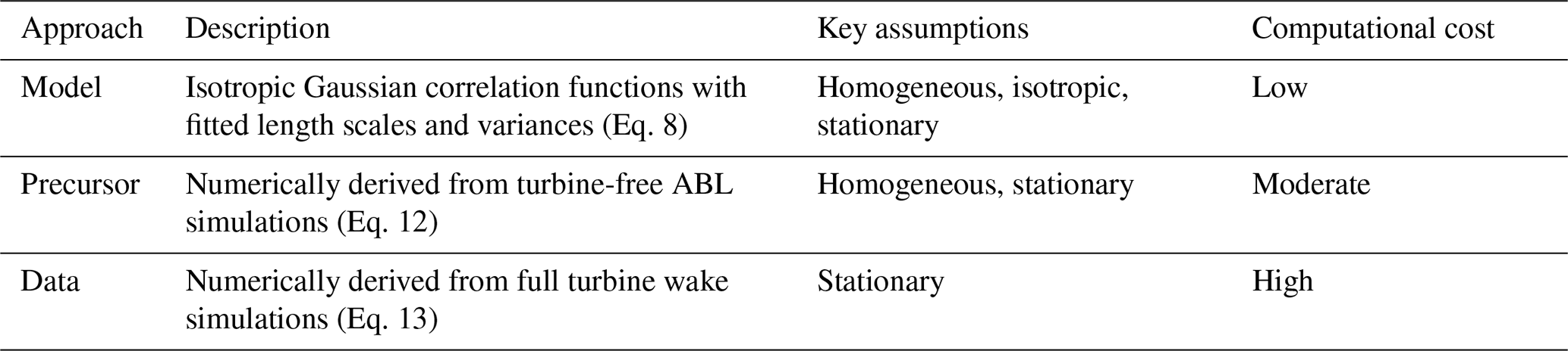
In Eq. (13), $\stackrel{\mathrm{‾}}{\mathit{u}}\left(\mathit{x}\right)$ is the advection velocity at point r^′. In practice, the simulated wind turbine wake is considered to be stationary in time, and the ensemble average is effectively identical to a time average over the simulation time. The model–data and data–data matrices can now be computed as before by integrating the numerically derived correlation functions $C_{{\mathit{\varphi }}_a{\mathit{\varphi }}_b}$ in place of the analytical functions supplied in Eq. (8).

It is important to note that this formulation does not normalize the correlation function by the value of C where $\mathit{r}{}^{\prime }=\mathit{r}$ and Δt=0, as is typically done to define the correlation coefficient. The correlation must retain its physical units to provide an accurate estimate of the fluctuating fields ϕ in the model domain, as normalization would remove the amplitude information necessary for proper field reconstruction (Wilson et al., 2008).

Table 1 Summary of covariance model approaches used in this study.

3 Problem setup

We conduct LESs of a Vestas V27 wind turbine (Petersen, 1990), operating in two distinct states corresponding to the neutral and convective ABL conditions. The simulations provide high-fidelity, dynamically consistent velocity and temperature fields, which serve as the foundation for evaluating acoustic tomography methods in wind energy. By resolving turbulence-driven covariances within the ABL and wind turbine wakes, we generate benchmark datasets to test retrieval accuracy against classical tomographic inverse assumptions. The turbine considered has a rotor diameter D=27 m, hub height H=31.5 m, rated wind speed of 14 m s⁻¹, and rated power output of 225 kW. Turbine-induced aerodynamic forces on the ABL flow are modeled using the Joukowski actuator disk model (Sørensen et al., 2020), which takes into consideration both the radial and tangential variations in the thrust loading across the rotor disk, improving fidelity compared to the traditional uniform-force actuator disk model implementations. The simulations are performed using AMR-Wind, a block-structured finite-volume solver built on the AMReX adaptive mesh refinement framework (Sprague et al., 2020; Zhang et al., 2021; Kuhn et al., 2025). The filtered continuity, momentum, and potential temperature equations are consistent with the formulation of Churchfield et al. (2012). Note that the buoyancy term is included via a reference potential temperature T₀=300 K. We close the subfilter-scale kinetic energy using Moeng's one-equation turbulence model (Moeng, 1984). Details on the numerical discretization are provided by Sharma et al. (2024) and Kuhn et al. (2025).

Table 2 ABL parameters for the neutral and convective cases.

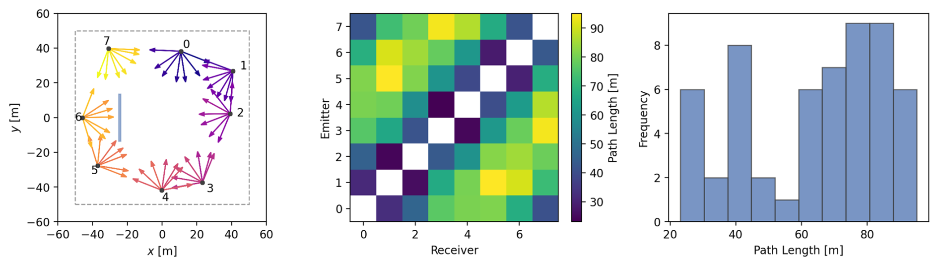
Figure 1 Layout of the collocated speakers (emitters) and microphones (receivers) in the virtual AT array used in the simulations (left), along with the travel time of acoustic signal along paths connecting emitter–receiver pairs (center) and a histogram of path lengths (right).

Table 3 Coordinates of the virtual AT array emission and/or reception points.

Figure 1 shows the layout of the virtual AT array used in the simulations. The subfigure on the left shows the eight emission and/or reception points (black points, detailed in Table 3), each associated with a set of seven vectors indicating the paths along which travel times are computed. The rotor of the modeled V27 is shown with a blue region centered at $(x,y)=(-\mathrm{25},\mathrm{0})$ m. The subdomain shown with a gray square is the area over which the fields are retrieved in the TDSI procedure, which is large enough to allow for information to advect downstream (to the right), as discussed in Sect. 2. The center figure describes the path length from each emitter (vertical axis) to each receiver (horizontal axis) in meters. The heatmap is symmetric along the main diagonal because virtual speakers and microphones are perfectly colocated in all simulation cases. The figure on the right shows a histogram of path lengths. Shorter paths correspond to neighboring emission and/or reception points, and longer paths tend to cross the domain. The virtual array is modeled as omnidirectional transceivers; loudspeakers operating in the 100–500 Hz range (wavelengths 0.7–3.4 m) are commercially available with near-omnidirectional directivity at these scales, consistent with this assumption (Hamilton and Maric, 2022; Maric et al., 2025). Travel-time synchronization between transceivers is assumed to be exact; in practice, GPS-disciplined clocking routinely achieves sub-millisecond timing accuracy sufficient for the path lengths considered here.

The computational domain for the simulations spans 3200 m in the streamwise (x) and lateral (y) directions. Vertically (z), the domain's height is 960 m for neutral ABL and 1600 m for convective cases. The larger height for the latter is meant to accommodate the deeper boundary layer under buoyant forcing. The turbine is positioned at $(x,y)=(\mathrm{1100},\mathrm{1600})$ m. Simulations have laterally periodic boundary conditions, a slip wall at the top, and a rough wall at the bottom. Laterally periodic conditions, while standard for idealized flat-terrain ABL simulations, are not expected to hold for complex terrain or non-stationary inflow conditions, which would require nested or precursor simulations with open lateral boundaries. The surface fluxes at the bottom wall are computed using the Monin–Obukhov similarity theory (Moeng, 1984), which is based on the friction velocity u^*, surface roughness z₀=0.1 m, and surface heat flux q₃|_w, which are set to 0 and 0.025 km s⁻¹ for the neutral and convective cases, respectively. Additionally, the von Kármán constant κ=0.4 (Table 2) summarizes the key ABL parameters, including the friction velocity, u^*; Obukhov length, L; and boundary layer height, δ. To maintain a target velocity of 7 m s⁻¹ at the hub height plane, a body force is applied as a driving pressure gradient. Near the lower surface, we introduce small perturbations to expedite boundary layer spin-up to quasi-equilibrium. Both the neutral and convective cases were initialized with a vertically uniform potential temperature T=300 K. A 100 m capping inversion layer follows, in which temperature increases linearly to 308 K. Above this, in the stable free atmosphere, we impose a constant lapse rate of 0.003 K m⁻¹. In the axial direction, the left and right boundaries are treated as mass inflow and pressure outflow, respectively. The turbulent inflow is generated a priori by running precursor simulations, where data of the flow variables are saved on a plane at each time step. The precursor runs consisted of a base mesh with grid resolution Δ=10 m and an additional refinement region that spans the entire x–y plane and extends up to z=80 m. In AMR-Wind, each layer of grid refinement reduces the grid spacing by a factor of half. Figure 2 shows the precursor-generated inflow boundary layer profiles up to a height of 100 m above the ground level, including a shaded region for the swept area of the rotor and a dashed line for the hub height of the simulated turbine.

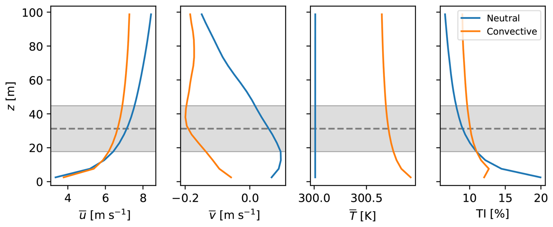
Figure 2 Inflow profiles of average horizontal velocity components, temperature, and turbulence intensity (TI) for the neutral and convective inflow cases. Shaded region and dashed horizontal line indicate the rotor-swept area and hub height of the V27 turbine, respectively.

Prior to running the suite of LESs for generating the covariance field data, we performed a mesh resolution study for the neutral ABL condition. The effect of three grid resolutions, referred to as coarse, medium, and fine, on the turbulence wake statistics was investigated. The coarse grid consisted of two layers of refinement, whereas the medium and fine grids had three and four refinement zones, respectively. For each case, the finest refinement block was centered at the turbine's hub height. It spanned −3D to 15D in the streamwise direction, ±7D in the lateral direction, and up to 80 m in the vertical direction. The corresponding actuator disk parameters are presented in Table 4, which includes the point force distribution width (ϵ), number of actuator points (“AP” in the table) for the disk radius, disk grid spacing (dr), and the ratio the two ($\mathit{ϵ}/\mathrm{dr}$). We chose $\mathit{ϵ}/\mathrm{\Delta }=\mathrm{2}$, and the number of radial grid points (actuator points) was chosen such that $\mathit{ϵ}/\mathrm{dr}>\mathrm{1}$. The wake statistics for all three meshes showed grid independency with the medium and fine grids. However, to ensure maximum resolution of the LES-based covariance fields, the results were obtained on the fine grid.

Table 4 Joukowski actuator disk parameters for the coarse, medium, and fine grids.

4 Results

The original TDSI formulation assumes homogeneous and stationary correlation functions. The analytical expressions in Eq. (8) impose horizontal homogeneity, such that the covariance depends only on the separation $\mathit{r}-\mathit{r}{}^{\prime }$. In the undisturbed ABL, free from topography, turbine wakes, or transient forcing, this assumption may be reasonable. However, Vecherin et al. (2006) also proposed deriving covariances from numerical simulations, which are not bound by these assumptions. Stationarity may still hold for turbine wakes, assuming sufficient ensemble averaging over the rotor-induced periodic forcing. Homogeneity, however, is more problematic. Aerodynamic forcing from the turbine induces strong inhomogeneities in the flow, including a persistent thrust-directed momentum deficit (Chamorro and Porté-Agel, 2010; Lignarolo et al., 2015). As a result, covariances between velocity and temperature fluctuations vary significantly with position and cannot be described solely by separation distance.

The results that follow quantify the impact of covariance model choice on the reconstruction of fluctuating velocity and temperature fields. We compare analytical models for the correlation functions, statistically stationary correlation functions calculated from the undisturbed ABLs represented by precursor simulations, and heterogeneous correlation functions for the turbine-influenced flows. Reconstructions are evaluated in a 100 m × 100 m two-dimensional plane at the V27 hub height.

4.1 Acoustic tomography retrievals of the inflow ABL cases

The precursor simulations represent neutral and convective ABL flow without wind turbine influence. These simulations yield velocity and temperature fields that are horizontally homogeneous, as are the associated two-point correlation functions. Negative values in the spatial correlation functions signal antiphase relationships between points, potentially reflecting the influence of coherent structures such as counter-rotating eddies that induce opposing velocity perturbations across the separation vector.

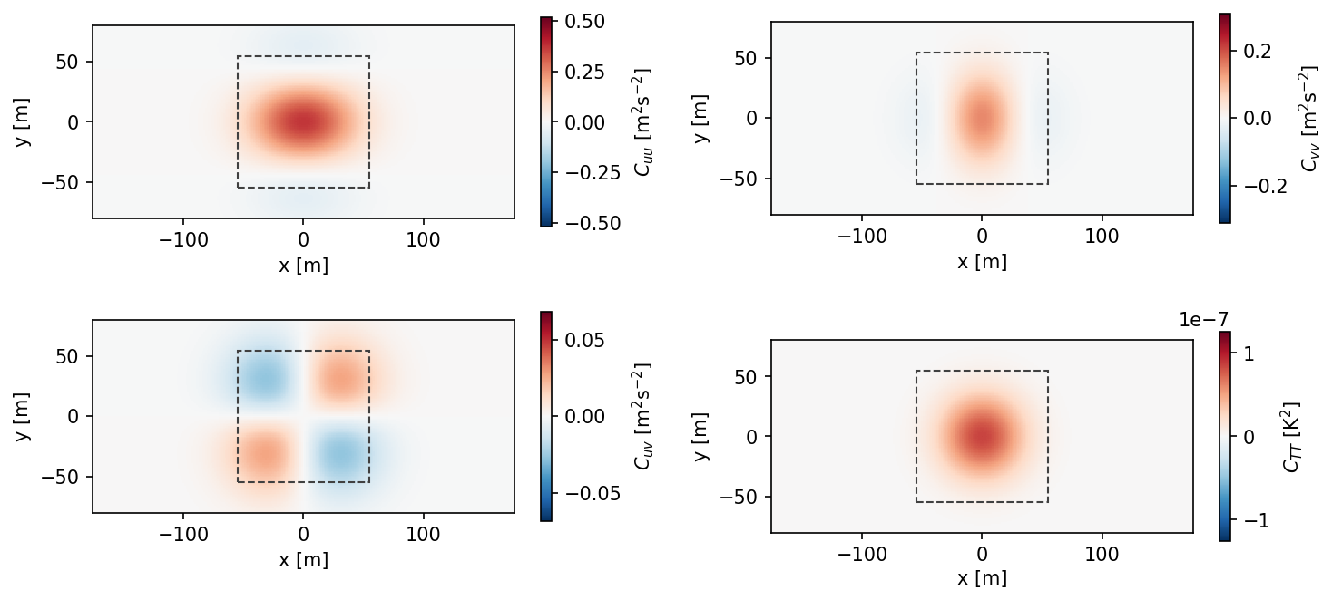
In the convective case (Fig. 3), the diagonal components of the correlation tensor – C_uu, C_vv, and C_TT – each exhibit a strong peak at Δr=0 that decays with increasing Δr. The decay of C_vv is approximately isotropic, while C_uu and C_TT show marked anisotropy with slower decay in the x direction than in the y direction. The cross-correlation C_uv exhibits a more complex structure. Shown in the lower-left panel of Fig. 3, C_uv contains alternating regions of positive and negative correlation.

The cross-covariance C_uv is an order of magnitude smaller than the corresponding variances C_uu and C_vv, indicating weak coupling between u^′ and v^′ fluctuations. The pattern is approximately antisymmetric about the x axis, with positive correlation in quadrants 1 and 3 and negative correlation in quadrants 2 and 4. However, the field shows less antisymmetry about the y axis, with stronger correlations for negative x. This asymmetry persists despite averaging over 600 s of simulation data. The dashed square in Fig. 3 indicates the 100 m × 100 m retrieval domain used for all reconstructions. This domain corresponds to the physical scale of the acoustic tomography array deployed at the National Laboratory of the Rockies' (NLR's) Flatirons Campus in Colorado, USA (Hamilton and Maric, 2022; Maric et al., 2025). The temperature covariance C_TT exhibits even lower magnitudes, which may imply that temperature fluctuations T^′ are minimal or uncorrelated at the measured scales. Similar correlation results for the neutral ABL case are shown in Sect. A but are not discussed in the current section for brevity.

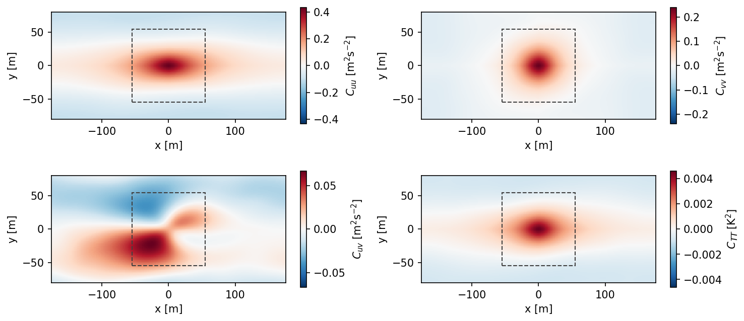
Figure 3 Two-point correlation functions of the convective precursor simulation. Dashed region indicates the domain of the fluctuating field retrievals.

Figure 4 shows the modeled correlation functions for the convective precursor, using optimal parameters listed in Table 5. However, it tends to exaggerate the extent of anticorrelation compared to the LES-based correlation, suggesting that the imposed functional form may be too rigid to capture the observed decay of correlations with increasing Δr.

The analytical correlation functions defined in Eq. (8) reproduce several key features of the convective precursor flow but also introduce important limitations. Notably, they impose anticorrelated regions in C_uu, outside of $\left|y\right|>\mathrm{45}$ m for the parameter values listed in Table 5, consistent with expectations from the form of the modulating function. The formulation from Vecherin et al. (2006) implies similar behavior for C_vv in the x direction, although the calculated covariances appear to be approximately isotropic.

The mismatch between calculated and modeled covariance is more pronounced in C_TT. While the simulation reveals gradual streamwise decay and the emergence of anticorrelated regions at large cross-stream distances, the analytical model fails to reproduce this structure. This discrepancy arises because the modulating function used for C_TT remains identically unity, precluding any sign reversal in the correlation field.

For the cross-correlation C_uv, the analytical model exhibits perfect antisymmetry about both the x and y axes, consistent with the mathematical constraints embedded in Eq. (9). In contrast, the LES-derived C_uv shows clear asymmetries, particularly about the y axis, highlighting the presence of directional flow structures that violate the assumptions of homogeneity and isotropy.

To quantify the match between modeled and simulated covariances, we optimize the model parameters by minimizing the normalized root-mean-square error (NRMSE), defined as

$$\begin{array}{}\text{(14)}& \text{NRMSE}=\sqrt{\sum _{i=\mathrm{1}}^M{\displaystyle \frac{({\mathit{\varphi }}_a-{\widehat{\mathit{\varphi }}}_a{)}^{\mathrm{2}}}{{\mathit{\varphi }}_a^{\mathrm{2}}}}},\end{array}$$

where ϕ_a signifies one of the fluctuating fields from the LES, the hat notation indicates the estimate of the field from the acoustic tomography retrieval, and M is the number of points in the domain. For temperature fluctuations, we report the simple root-mean-square error (RMSE) rather than NRMSE because the normalization by standard deviation obscures meaningful comparison when temperature variability is small, particularly in the neutral ABL, where ${\mathit{\sigma }}_T\approx {\mathrm{10}}^{-\mathrm{4}}$ K. Table 5 summarizes the resulting best-fit parameters for u, v, and T under both convective and neutral conditions. Unlike the original TDSI formulation, which assumes a common parameter set across all fields, we allow each field to adopt its own optimal values. This added flexibility enables better agreement with the LES data, particularly in flows with strong directional anisotropy or field-specific spatial structure.

Table 5 Optimal model parameters σ_ϕ and l_ϕ for convective and neutral conditions in precursor and turbine cases.

Figure 4 Modeled correlation functions from Eq. (8) for the convective case tuned to match numerical correlation functions for the convective precursor shown in Fig. 3. Model parameters correspond to those listed in Table 5.

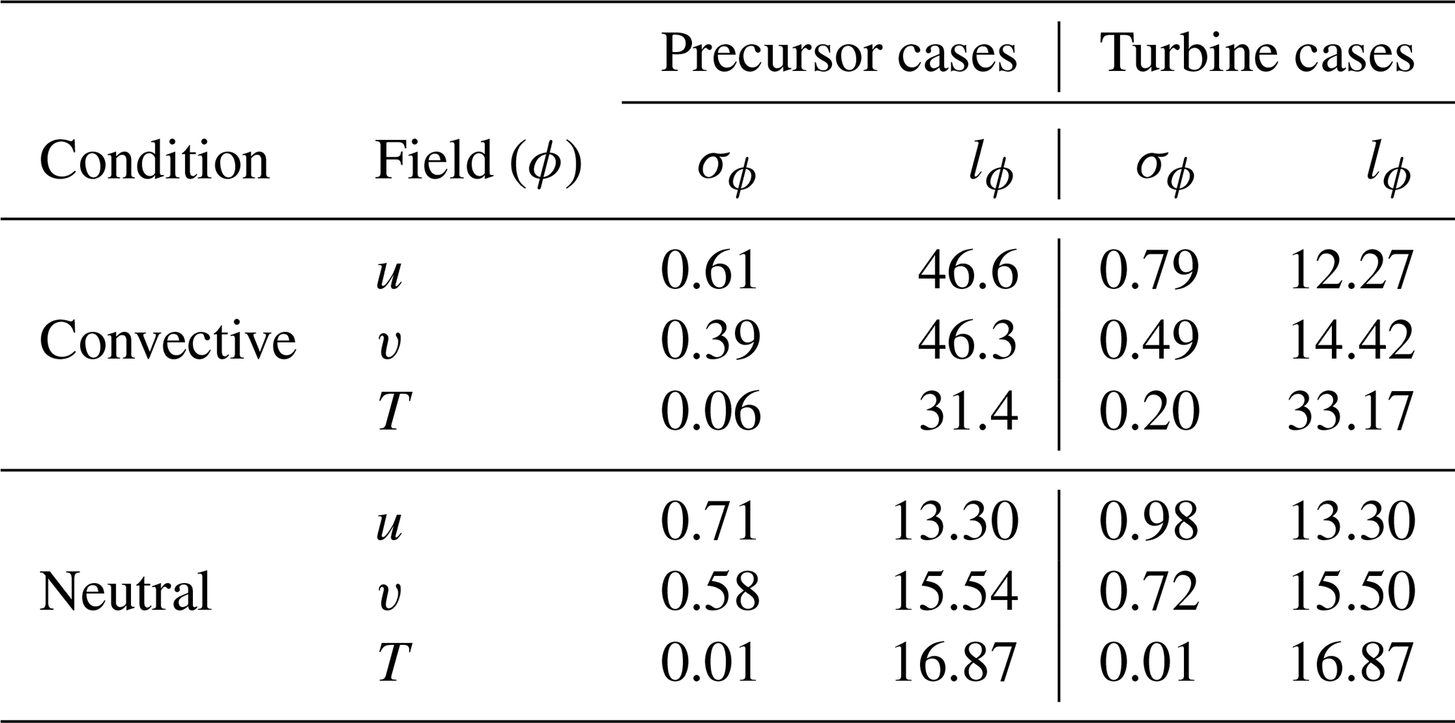
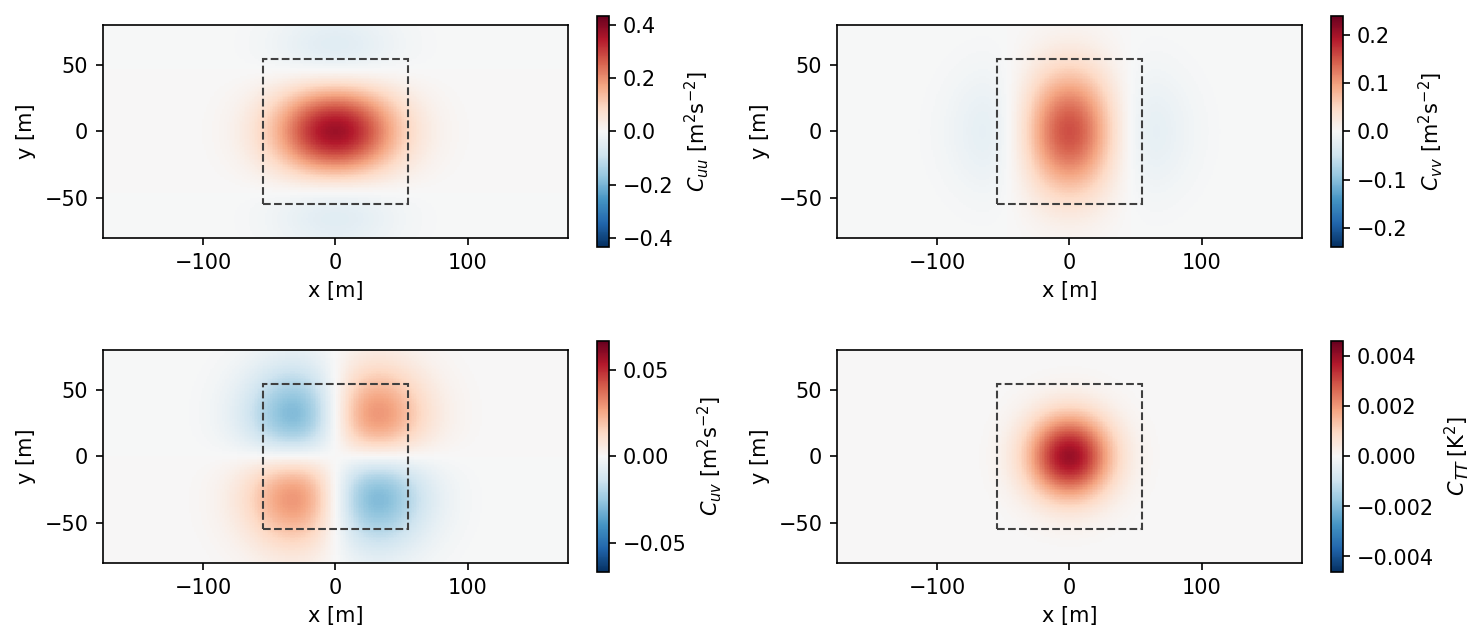
Figure 5 presents a snapshot comparison of the fluctuating streamwise velocity component, u^′, from the convective precursor simulation (left), alongside retrievals based on the numerically derived (middle) and analytically modeled (right) correlation functions. All reconstructions use N_f=4, incorporating two acoustic observations before and two after the retrieval time. Both retrievals exhibit strong qualitative agreement with the simulated field, accurately recovering the dominant spatial structures. Key features, such as the regions of negative u^′ near the top and bottom boundaries and a localized positive patch centered near $(x,y)=(-\mathrm{40},-\mathrm{10})$ m, are present in both reconstructed fields.

Despite the similarities for large-scale features, differences emerge at smaller scales. The reconstruction based on numerically derived correlations (middle) more faithfully reproduces secondary features, including small-magnitude fluctuations near the center of the domain and the peak positive excursion of u^′. However, it slightly overshoots the negative peak near the upper boundary, indicating a local mismatch in amplitude. In contrast, the retrieval using modeled covariances (right) introduces small-scale oscillations not observed in the simulation. These spurious features likely result from the interaction between the assumed covariance structure and the inclusion of multiple time-separated observations in the stochastic inverse operator A.

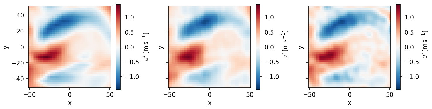
Figure 5 Comparison of the u^′ from the convective precursor LES (left) to the retrievals with the numerical correlations (middle) and the modeled covariances (right).

Figure 6 quantifies these retrieval differences by showing distributions of NRMSE across an ensemble of retrievals with varying numbers of successive frames. Darker curves correspond to reconstructions using fewer frames (smaller N_f), while lighter curves reflect increasingly wider temporal windows. For both the convective (Fig. 6) and neutral (Fig. 6) cases, the left panels show retrieval error using numerically derived correlations, and the right panels show results using the modeled correlation functions. In both cases, retrievals using numerical correlations consistently outperform their analytical counterparts, particularly as N_f increases. This suggests that while both covariance models support accurate large-scale reconstructions, the numerically derived correlations yield more faithful representations of the spatiotemporal variability embedded in the LES data.

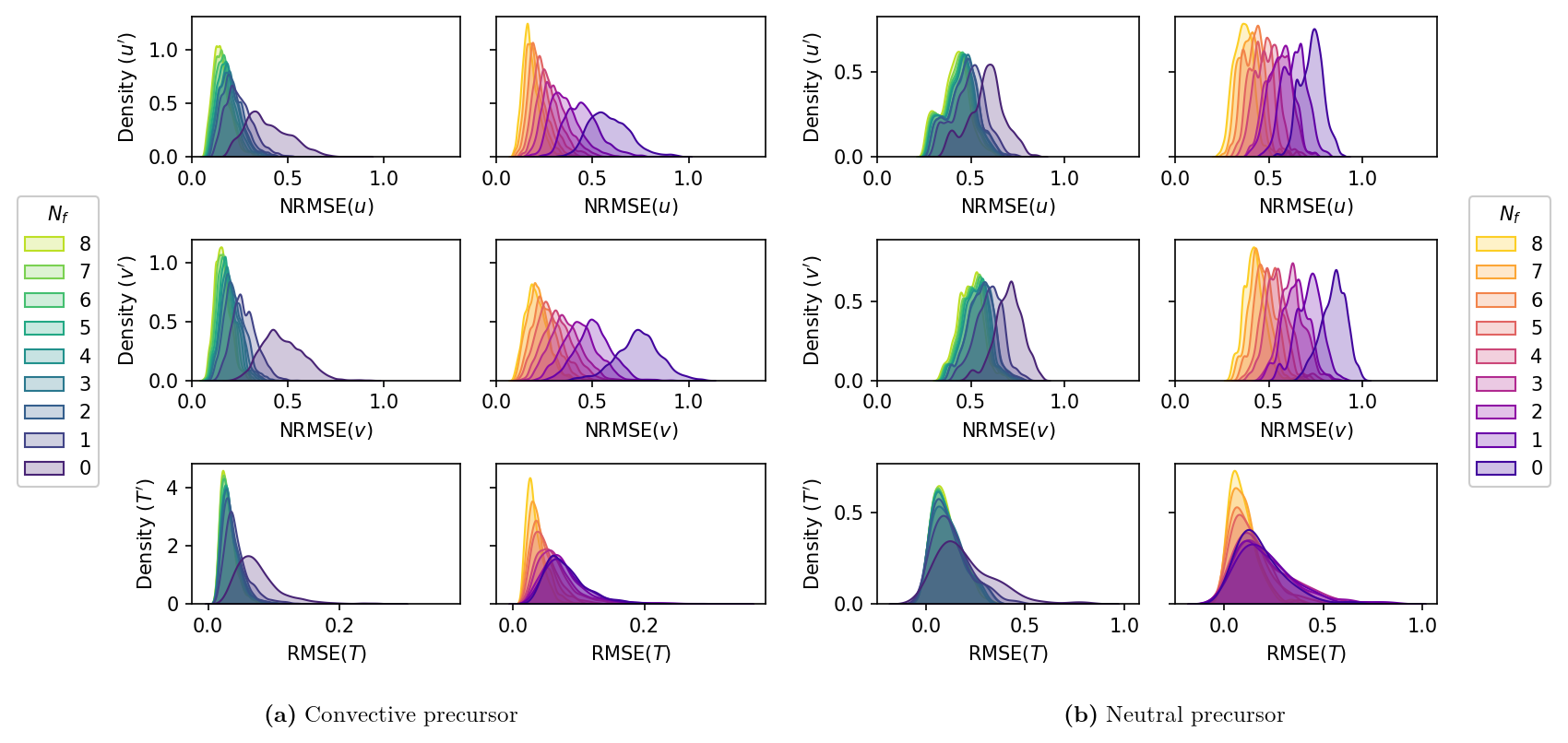
Figure 6 Distributions of error metrics for the convective (a) and neutral (b) precursor simulations considering the calculated and analytically modeled correlation functions (left and right column of each subfigure) for u^′ (top), v^′ (middle), and T^′ (bottom) field variables. NRMSE is shown for velocity components; RMSE (K) is shown for temperature.

For the convective case, retrievals based on numerically derived covariance fields show a rapid decline in NRMSE as the number of successive frames increases from N_f=0 to N_f=2. This initial improvement reflects the added value of incorporating temporal information from observations one time step before and after the retrieval time. Beyond N_f=2, further increases in the observation window offer diminishing returns. The NRMSE levels off for retrieved fields $\widehat{u}{}^{\prime }$, $\widehat{v}{}^{\prime }$, and $\widehat{T}{}^{\prime }$, shown in the left column of Fig. 6.

In contrast, retrievals using the modeled correlation functions exhibit consistently higher NRMSE for $\widehat{u}{}^{\prime }$ and $\widehat{v}{}^{\prime }$, particularly at small N_f. While retrieval accuracy improves with additional frames, the rate of error reduction is more gradual and persists over a broader range of N_f, suggesting that the modeled covariances benefit more from temporal averaging than their data-driven counterparts.

For the neutral case (Fig. 6), retrieval error trends for u^′ and v^′ mirror those observed in the convective ABL and NRMSE and drop sharply as N_f increases. However, unlike in the convective regime, the spread of NRMSE distributions remains nearly constant with increasing N_f, simply shifting toward lower median values. This persistent variability suggests that retrieval performance is more sensitive to specific observation configurations or flow states in the neutral ABL, possibly due to its more isotropic structure.

The RMSE of temperature fluctuations shows similar overall trends to the NRMSE of the velocity fluctuations, where the mean and standard deviation of the error decreases as N_f is increased. Again, the temperature is described in terms of RMSE rather than NRMSE because the standard deviation of temperature fluctuations is very small, particularly in the neutral ABL, which would lead to artificially inflated NRMSE values. Accordingly, both the mean and standard deviations of the RMSE of T^′ are lower for the convective case than for the neutral case, regardless of the covariance model used. These distributions highlight both greater retrieval uncertainty and weaker observational sensitivity to temperature fluctuations. This trend aligns with prior findings from Vecherin et al. (2006) and Maric et al. (2025) and underscores the inherent limitations of acoustic tomography for inferring temperature. In the neutral ABL, the median RMSE for T^′ reveals that errors in the retrievals of temperature fluctuations are on the order of 0.25 K, which is likely the practical resolution limit of acoustic tomography. Two factors contribute to poor temperature retrieval performance in neutral conditions. First, the imposed surface heat flux is set to zero, resulting in negligible temperature variability. Second, the TDSI framework is intrinsically limited in resolving temperature fluctuations below approximately 0.1 K, as previously reported by Maric et al. (2025).

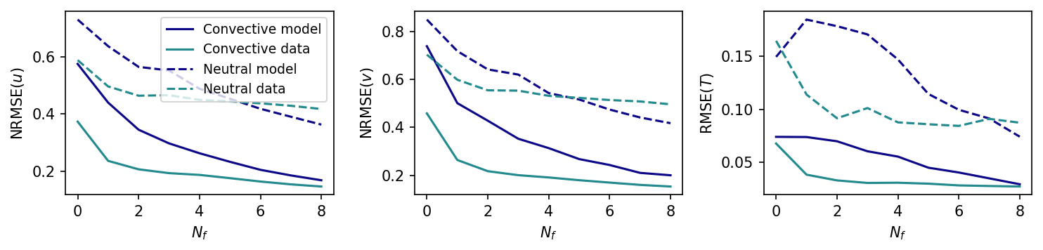
Figure 7 Median values of error metrics as a function of N_f for u^′ (left), v^′ (center), and T^′ (right). NRMSE is shown for velocity components; RMSE (K) is shown for temperature.

Figure 7 compares the median error metrics across retrieved fields $\widehat{u}{}^{\prime }$, $\widehat{v}{}^{\prime }$, and $\widehat{T}{}^{\prime }$ as a function of the number of frames N_f used in the stochastic inverse operator A. Solid lines represent convective cases, dashed lines indicate neutral cases, and color denotes the source of the correlation functions: green for numerical correlations and purple for analytical models. In both ABL cases, retrievals based on numerical covariances (green) exhibit minimal improvement in retrieval accuracy beyond N_f=4, suggesting that additional temporal information adds little value once short-term correlations are resolved. In contrast, retrievals using modeled covariances (purple) show a gradual and consistent improvement with increasing N_f, highlighting their greater sensitivity to temporal averaging.

For the convective ABL (solid lines), modeled correlations consistently produce higher errors than their numerical counterparts for all variables when N_f≤8. This disparity indicates that the modeled functions lack sufficient fidelity to represent the fine-scale variability in the LES data without additional observational context. For the neutral ABL (dashed lines), however, the trends differ. Here, modeled correlations begin to outperform numerical covariances for $\widehat{u}{}^{\prime }$ and $\widehat{v}{}^{\prime }$ when N_f≥5 and for $\widehat{T}{}^{\prime }$ when N_f≥6. This crossover may reflect the smoother, more isotropic character of the neutral ABL, which is more consistent with the assumptions embedded in the analytical model and may benefit more from increased temporal integration.

4.2 Wind turbine wake retrievals

Wind turbine wakes are considerably more complex than the horizontally homogeneous ABL flows described in the previous section. The presence of the rotor disk and associated aerodynamic forcing makes the flow strongly inhomogeneous, with marked spatial variation in mean fields and the higher-order statistics used in acoustic tomography. Figure 8 presents the triple decomposition of the streamwise velocity u for the convective ABL case introduced in Eq. (10). The instantaneous field (top left) captures the full spatial variability in the flow at a single time. The time-averaged velocity field $\stackrel{\mathrm{‾}}{u}$ (top right) reveals persistent features, including an upstream deceleration due to induction and a pronounced wake extending more than 250 m downstream of the rotor. These structures are absent in the spatially averaged time series (bottom left), which represent domain-wide averages over time and remain centered around zero. The purely fluctuating component u^′ (bottom right) isolates transient variations and exhibits an asymmetric structure, with $u{}^{\prime }>\mathrm{0}$ for y<0 and $u{}^{\prime }<\mathrm{0}$ for y>0. This asymmetry indicates that the instantaneous wake deviates from its mean trajectory at the time of the snapshot shown in the figure. Dashed squares in each subfigure mark the 100 m × 100 m footprint of the physical acoustic tomography array deployed at the NLR Flatirons Campus (Hamilton and Maric, 2022). Gray lines denote the acoustic ray paths used in the retrieval process.

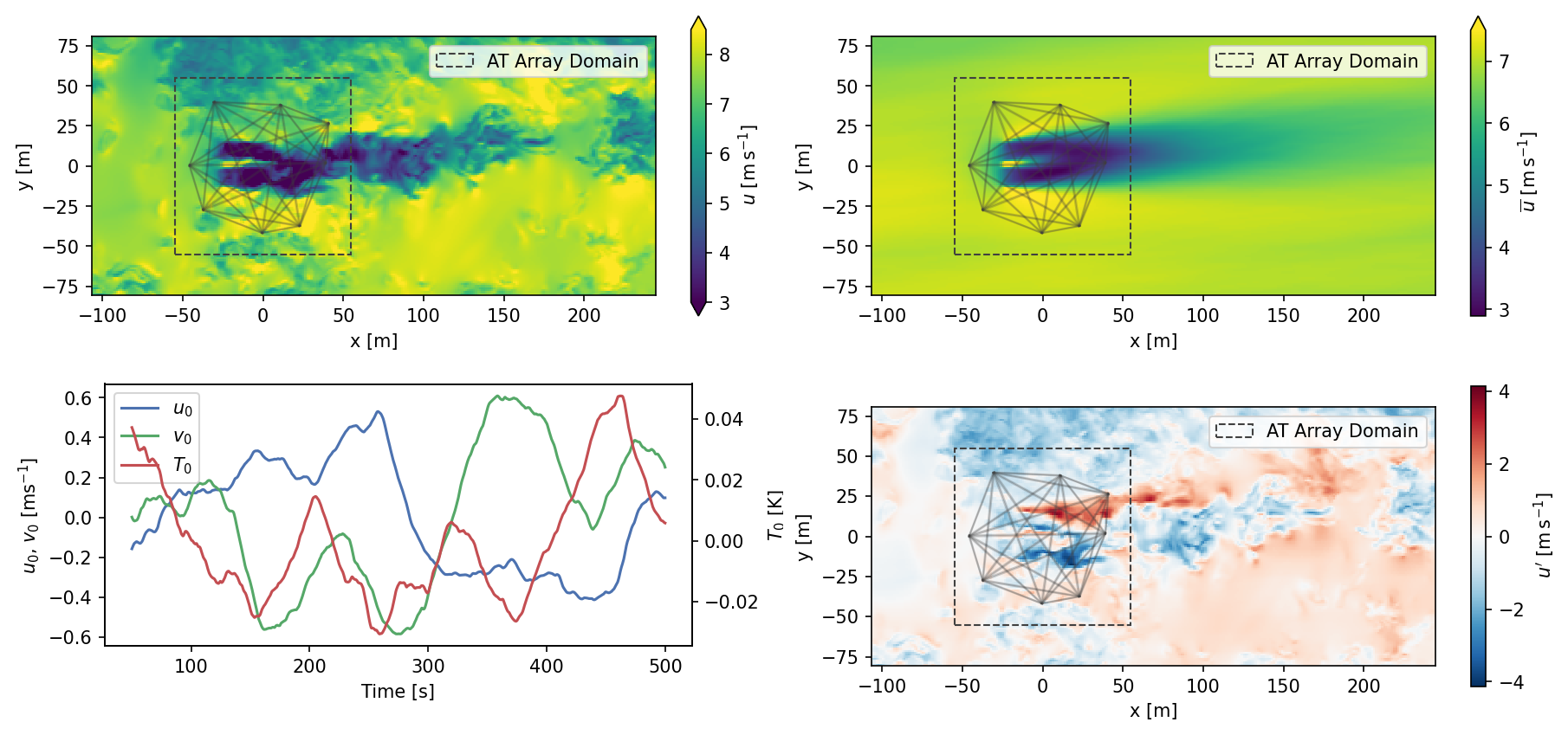
Figure 8 Convective simulation showing an instantaneous snapshot of the flow (top left) at hub height, time average field $\stackrel{\mathrm{‾}}{u}$ (top right), time series of spatial average velocity u₀ (bottom left), and the purely fluctuating component u^′ (bottom right).

Figure 9 presents the same triple decomposition of the streamwise velocity u for the neutral ABL case. Compared to the convective case, the time-averaged wake in the neutral ABL is more well defined, exhibiting a sharper momentum deficit and a more distinct upstream deceleration due to the induction zone. The background flow is notably more uniform, with $\stackrel{\mathrm{‾}}{u}\approx \mathrm{8}$ m s⁻¹ across most of the domain outside the wake. As in the convective case, the spatially averaged time series, u₀, v₀, and T₀, remain centered near zero. However, they span a smaller range of variability: u₀ and v₀ fluctuate within approximately ±0.5 m s⁻¹, while T₀ varies only between −0.0003 and 0.0005 K. To maintain focus, the following discussion limits reference to the neutral case and to aggregated metrics that can be directly compared to the convective case. Readers interested in a more detailed treatment of the neutral wake are referred to Sect. A.

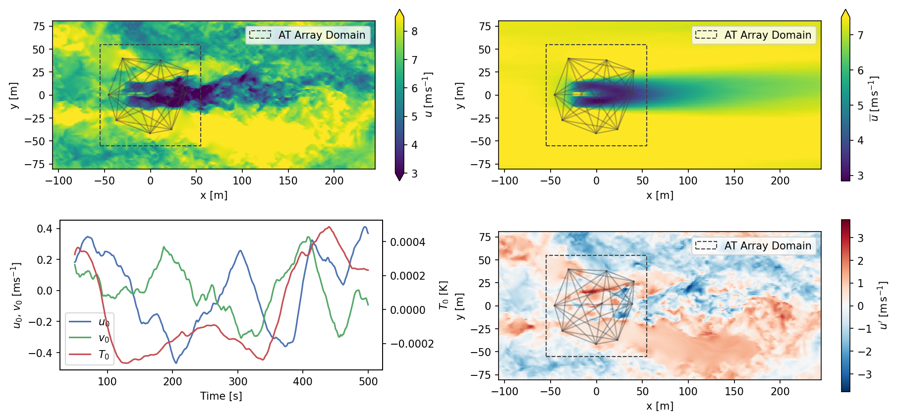
Figure 9 Neutral simulation showing an instantaneous snapshot of the flow (top left) at hub height, time average field $\stackrel{\mathrm{‾}}{u}$ (top right), time series of spatial average velocity u₀ (bottom left), and the purely fluctuating component u^′ (bottom right).

Because the turbine wakes are strongly inhomogeneous, the correlation functions derived from simulation data cannot be expressed in simplified, stationary form. Instead, they depend explicitly on the locations of both points r and r^′, requiring the correlation function to be computed independently for every pair in the domain. As a result, each component of the covariance tensor becomes a full M×M field, where M is the number of grid points in the domain.

A representative set of correlation functions for the convective turbine case is shown in Fig. 10. Each subplot visualizes the correlation between the point marked in green with every other point in the domain, located along y=0 and positioned at $x/D\in [-\mathrm{1},\mathrm{0},\mathrm{1},\mathrm{2}]$. The color scales are normalized independently for each reference location to better highlight local structure and scale.

.

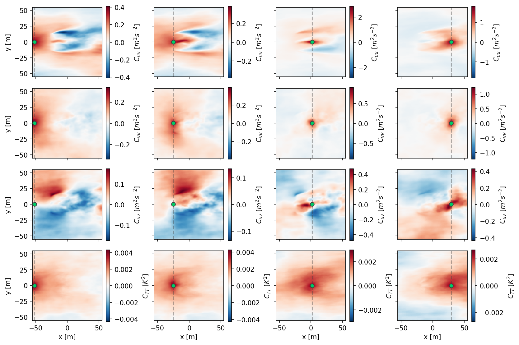
Figure 10 Examples of the correlation functions for the convective wind turbine wake case. The central point (r) for each plot is indicated with a green marker. Vertical dashed gray lines indicate transects for which profiles are compared in Fig. 12.

The autocorrelation C_uu exhibits an order-of-magnitude increase from the inflow to the wake: while fluctuations upstream are weakly correlated with maximum values around ±0.4 m² s⁻², near-wake regions reach peak correlations exceeding ±2.5 m² s⁻², reflecting the emergence of coherent, periodic fluctuations induced by the rotor. Notably, the contours of C_uu reveal the spatial imprint of the wake, with clear anticorrelation between the wake and upstream flow. At x=2 (one rotor diameter downstream of the actuator disk), the correlation structure across the wake is asymmetric: one edge of the wake remains positively correlated with the centerline, while the opposite side exhibits negative correlations – an imprint of rotational asymmetry induced by the turbine. In contrast, C_vv – the autocorrelation of the cross-stream velocity component – shows a broader correlation length scale in the inflow and much weaker correlations within the wake. For the points within the wake highlighted in the second row of Fig. 10, C_vv appears nearly isotropic but decays rapidly, indicating short-lived and small-scale fluctuations.

The cross-correlations C_uv capture the intricate coupling between streamwise and cross-stream velocity components and highlight features that are particularly challenging for simplified models to replicate. The most significant correlations cluster around the rotor disk, where C_uv>0 for y>0 and C_uv<0 for y<0. This antisymmetric pattern points to the bulk flow rotation introduced by the rotor and continues to shape local velocity interactions downstream. Temperature correlations, C_TT, show fundamentally different behavior than the velocity fields. Despite the strong inhomogeneity in velocity, C_TT remains spatially consistent across the domain, with little indication that the presence of the turbine significantly alters the magnitude or structure of thermal fluctuations. This suggests that the turbine's impact is largely mechanical and that thermal perturbations are governed by broader boundary layer processes.

To complement the LES-based correlation functions, modeled correlation functions were again constructed using the analytical form in Eq. (8). Unlike the precursor case – where the model parameters were tuned to minimize the error between analytical and numerical correlations – here the parameters were selected to minimize the median NRMSE between retrieved and simulated fields. This shift in focus reflects the goal of improving retrieval fidelity rather than exact reproduction of the underlying statistics. Model parameters for the actuator disk simulation cases are listed in Table 5 under the “Turbine cases” column.

Figure 11 shows the resulting modeled correlation functions for the convective turbine case. The optimized length scales are uniformly smaller than those derived for the precursor flows. This contraction in spatial coherence likely reflects the smaller turbulent length scales present within and around the wake.

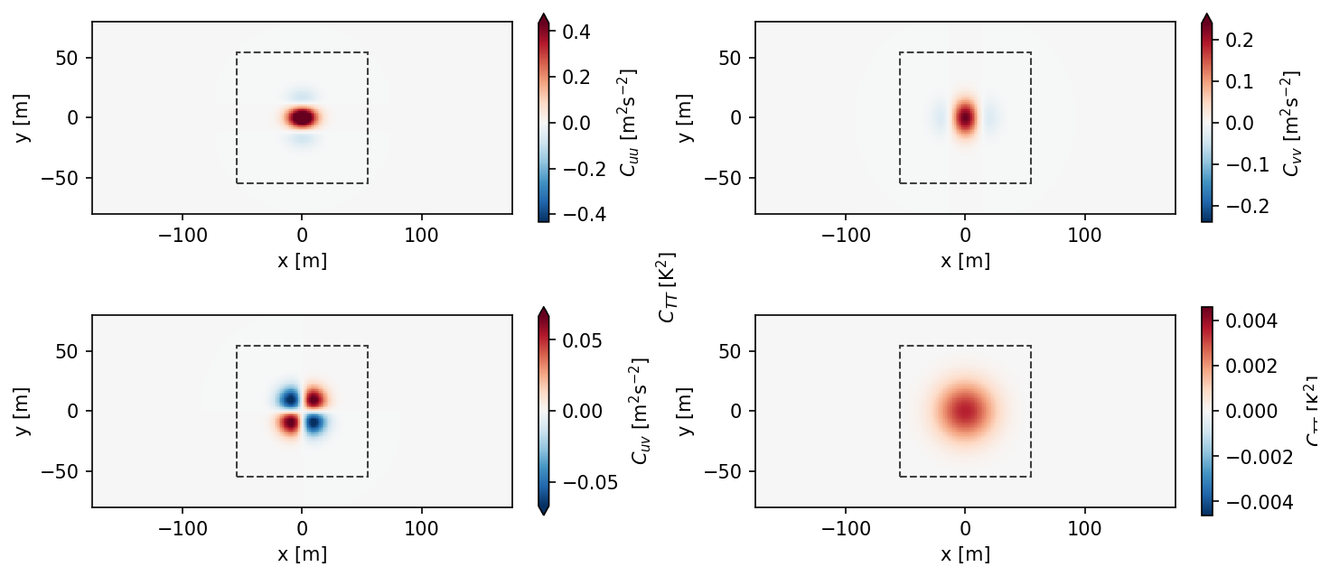
Figure 11 Modeled correlation functions for the convective case optimized to minimize reconstruction error, ε, in the convective turbine simulation.

To aid visual comparison between the correlations, Fig. 12 contrasts cross-sections of the correlation functions C_uu, C_vv, and C_TT at various streamwise locations with correlation functions from the precursor (Fig. 3) and the NRMSE-minimizing modeled correlations (Fig. 11) for both the convective and neutral cases. C_uv is not shown in the figure, as the model forces this component to be zero along horizontal and vertical transects that include r, which makes it difficult to compare to the results computed from simulations.

Correlations C_uu and C_vv (left and middle columns, respectively) show close agreement between the numerical and modeled correlations upstream of the rotor plane for transects at $x/D\le \mathrm{0}$ in both stability regimes. In contrast, the correlation functions in the wake region differ substantially in both magnitude and structure. The periodic forcing imposed by the rotor blades, represented as a radially distributed body force in the actuator disk model, leads to enhanced spatial coherence in velocity fluctuations, particularly in the near-wake, $x/D\lesssim \mathrm{3}$.

Similar to the observations in Placidi et al. (2023), the largest peaks in C_uu and C_vv are observed directly downstream of the rotor hub, centered at $y/D=\mathrm{0}$. Secondary peaks occur along the horizontal edges of the rotor disk, between $y=\pm D/\mathrm{2}$ and $y=\pm D$, and exhibit antisymmetric deviations from the homogeneous distribution. This antisymmetry reflects the rotational influence introduced by the rotor, which deflects low-momentum flow upward toward hub height on one side (y<0) and draws high-momentum flow downward on the opposite side (y>0). As turbulence within the wake mixes the flow, these secondary peaks diminish, and the correlation structure becomes more isotropic, approaching that of the precursor. The secondary peaks in C_uu are more pronounced in the convective case than in the neutral case.

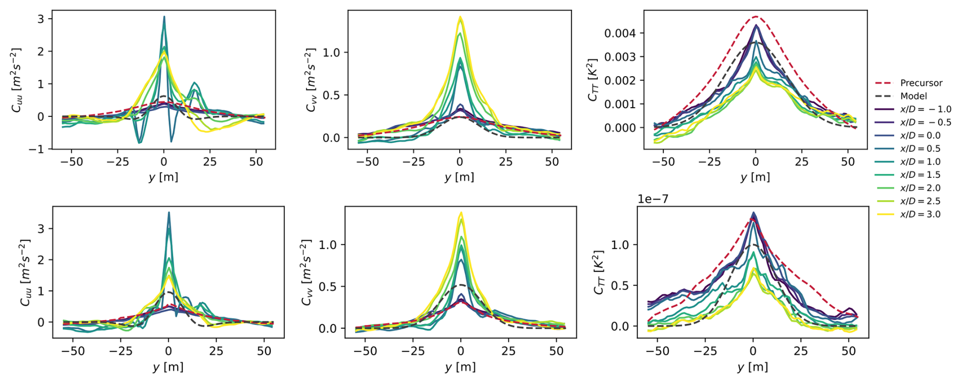
Figure 12 Comparison of correlation functions from the convective (top) and neutral (bottom) turbine simulations at various streamwise locations. Cross-sections of the correlation functions C_uu (left), C_vv (center), and C_TT (right) are compared to the respective homogeneous correlations from the precursor (red) and analytical model (black).

The shape and magnitude of C_TT remain much closer to those predicted by the precursor and the analytical model, even in the presence of the rotor. The rotor's influence on temperature fluctuations is comparatively weak, and the resulting correlation functions are nearly isotropic throughout the domain. Atmospheric stability still exerts a significant influence on C_TT. The convective case exhibits a substantially larger correlation length scale than the neutral case, consistent with the stronger vertical mixing associated with buoyancy-driven turbulence.

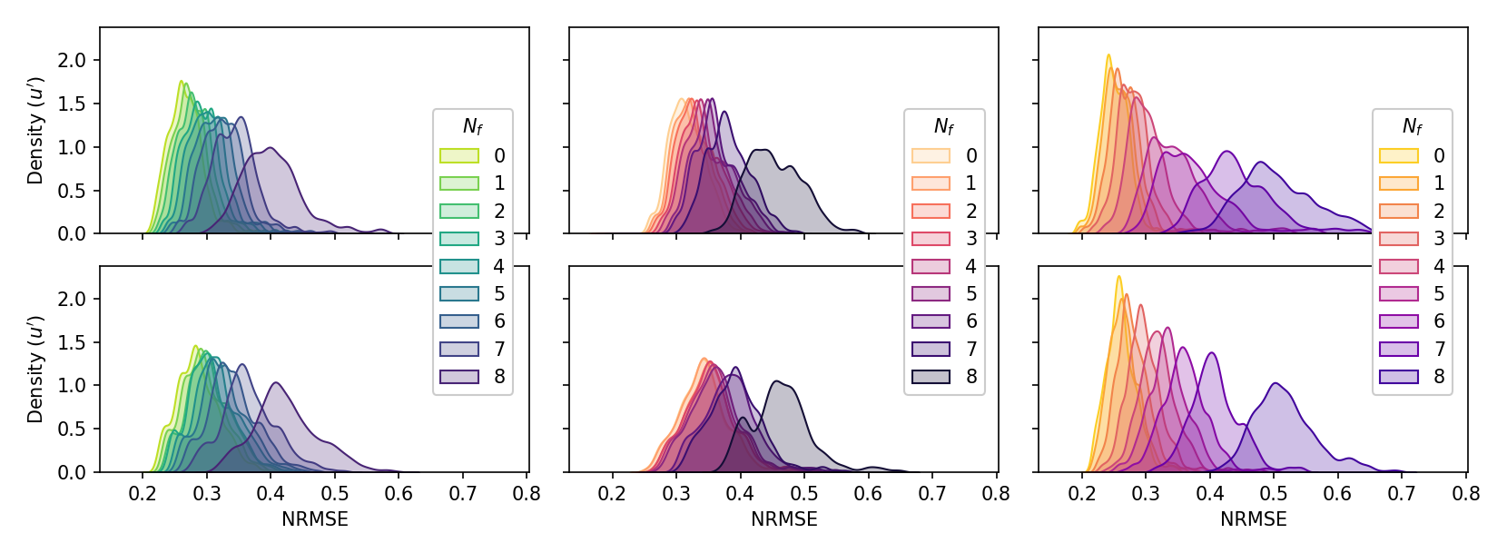
Figure 13 Distributions of the reconstruction error for AT retrievals of the u^′ component of velocity considering the convective (top row) and neutral (bottom row) flow cases. Error distributions correspond to use of the numerical correlation functions (left column), correlations from the respective precursor flows (center), and the modeled correlation functions (right column).

Figure 13 compares the NRMSE of retrievals $\widehat{u}{}^{\prime }$ using the three sources of covariance information: heterogeneous correlations from the turbine LES (left), homogeneous correlations from the precursor simulations (center), and analytical covariance models (right). As in Fig. 6, darker colors indicate retrievals based on fewer successive frames, N_f, and lighter colors correspond to retrievals incorporating more frames. For all covariance sources, the width of the NRMSE distributions decreases with increasing N_f, with N_f=0 exhibiting the broadest range. Distributions for v^′ and T^′ are omitted in Fig. 13 for clarity and brevity.

Figure 14 shows the median NRMSE values for u^′ as a function of N_f, with the convective case presented in the top row and the neutral case in the bottom row. Each subplot includes three trends: retrievals using covariances from the turbine LES (green), the precursor simulations (purple), and the analytical model (red). Consistent with trends observed in the precursor analysis, using heterogeneous covariance estimates from the turbine simulations yields the lowest median NRMSE up to N_f=4. For N_f>4, the analytical covariance model yields lower retrieval error than the numerical covariances, despite not explicitly capturing the wake heterogeneity. This crossover may be attributed to the improved conditioning of the mapping operator A when based on smoother, parameterized correlation functions and the accumulation of information from multiple successive observations that attenuate the effects of model mismatch.

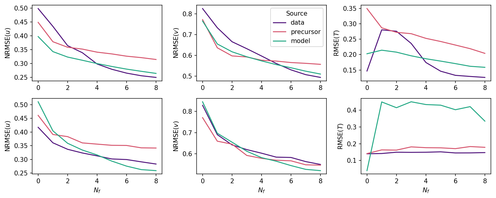
Figure 14 Median values of error metrics for u^′ (left), v^′ (center), and T^′ (right). The top row corresponds to convective atmospheric conditions, and the bottom row shows results for a neutral ABL. Each plot compares retrieval errors when defining A with the analytical models (purple), the homogeneous correlation functions from the precursors, or the heterogeneous correlation functions from the turbine simulations. NRMSE is shown for velocity components; RMSE is shown for temperature.

In both the convective and neutral turbine cases, the homogeneous estimate for covariances consistently produces higher NRMSE for $\widehat{u}{}^{\prime }$. This trend does not hold for retrievals of the spanwise velocity fluctuations, $\widehat{v}{}^{\prime }$. While the heterogeneous covariance estimates yield a lower median NRMSE than the analytical model at low values of N_f, as seen for $\widehat{u}{}^{\prime }$, the precursor estimates are approximately equal to, or better than, either of the other sources. This result is consistent with the selected cross-sections of $C_{vv}(\mathit{r},\mathit{r}{}^{\prime })$ shown in Fig. 12 (second row), where the spanwise velocity correlations are well approximated by the homogeneous precursor correlations shown in Fig. 3. Although the magnitude of C_vv varies by a factor of 2 depending on the choice of r, its spatial structure is approximately preserved in the homogeneous model.

The median RMSE for retrievals of temperature fluctuations, $\widehat{T}{}^{\prime }$, shows the most deviation from the monotonic decrease in retrieval error trend. In this case, the median RMSE increases substantially for both the heterogeneous and analytical correlation functions when using small ensembles of snapshots. Notably, the zero-lag case (N_f=0), corresponding to a stochastic inversion that does not include time dependence, outperforms low-N_f ensemble approaches. After reaching a maximum, the median RMSE begins to decrease again with increasing N_f, at N_f=1 for the heterogeneous case and N_f=2 for the analytical model in the convective case.

Temperature retrievals also exhibit the largest discrepancy in median RMSE between the convective and neutral stability cases. This difference arises from the boundary conditions used in the simulations. In the neutral ABL case, the imposed surface heat flux is set to zero, resulting in negligible kinematic heat flux and correspondingly weak temperature fluctuations on the order of 10⁻⁴ K. In contrast, the convective ABL case supports much stronger temperature fluctuations, several orders of magnitude larger, which are more amenable to retrieval. This is most clearly illustrated in the distributions of RMSE for the modeled temperature retrievals: the convective case converges to a median RMSE near 0.2 K, while the neutral case shows absolute errors on the order of 0.4 K.

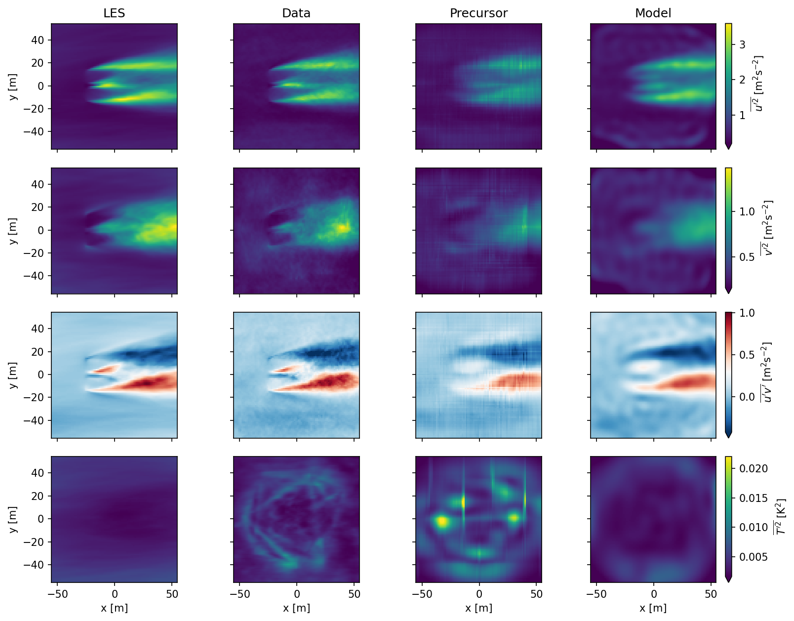
Figure 15 Comparison of the simulated streamwise and spanwise Reynolds normal stresses, the in-plane Reynolds shear stress, and the temperature variance (from top) to the AT retrievals for the convective case.

One of the key advantages of AT over other remote sensing methods for wind energy is its ability to resolve fluctuating velocity and temperature fields. To evaluate the quality of retrievals produced using the methods explored here, Fig. 15 compares the estimated in-plane Reynolds stresses and temperature variance to their counterparts from the LES (left column). All estimated variance fields qualitatively match the LES results, although each covariance model exhibits unique features. Retrievals using heterogeneous covariances derived from the turbine simulations (second column) show excellent agreement with the LES for $\stackrel{\mathrm{‾}}{{u^{\prime }}^{\mathrm{2}}}$, $\stackrel{\mathrm{‾}}{{v^{\prime }}^{\mathrm{2}}}$, and $\stackrel{\mathrm{‾}}{u{}^{\prime }v{}^{\prime }}$. However, the temperature variance $\stackrel{\mathrm{‾}}{{T^{\prime }}^{\mathrm{2}}}$ is overestimated along the acoustic signal travel paths. The estimate of $\stackrel{\mathrm{‾}}{{u^{\prime }}^{\mathrm{2}}}$ from the heterogeneous model also captures fine-scale structures around and downstream of the rotor that are absent from the fields reconstructed using precursor or analytical models.

Retrievals based on the precursor-derived correlation functions exhibit vertical striations in all variance estimates, which may arise from mismatches between the precursor and turbine flow statistics. This is most evident in $\stackrel{\mathrm{‾}}{{v^{\prime }}^{\mathrm{2}}}$ and $\stackrel{\mathrm{‾}}{u{}^{\prime }v{}^{\prime }}$, where the pattern suggests a spatial aliasing effect due to correlation function inaccuracies.

Retrievals using analytically modeled covariances (right column) reproduce the gross structure of all variance fields and generally agree with LES in magnitude. However, the Gaussian form of the analytical kernel leads to an apparent low-pass filtering effect, smoothing out small-scale structures that are evident in the LES. An additional limitation of the analytical covariance model is its inability to recover accurate estimates of fluctuations near the domain boundaries, far from the acoustic travel paths. This limitation has been noted in prior AT studies (e.g., Vecherin et al., 2006; Hamilton and Maric, 2022; Maric et al., 2025) and underscores the importance of sensor placement in AT system design.

Among all quantities, the temperature variance $\stackrel{\mathrm{‾}}{{T^{\prime }}^{\mathrm{2}}}$ (bottom row of Fig. 15) shows the greatest deviation from the LES. As discussed previously, temperature fluctuations in this convective case are largely decoupled from the dynamics of the rotor, and the temperature variance field is nearly isotropic. However, most AT-based estimates of $\stackrel{\mathrm{‾}}{{T^{\prime }}^{\mathrm{2}}}$ significantly exceed the LES values, except those derived from the analytical model. More importantly, both the heterogeneous and precursor-based covariance estimates introduce artifacts aligned with the acoustic paths, manifesting as spatially localized overestimates in temperature variance.

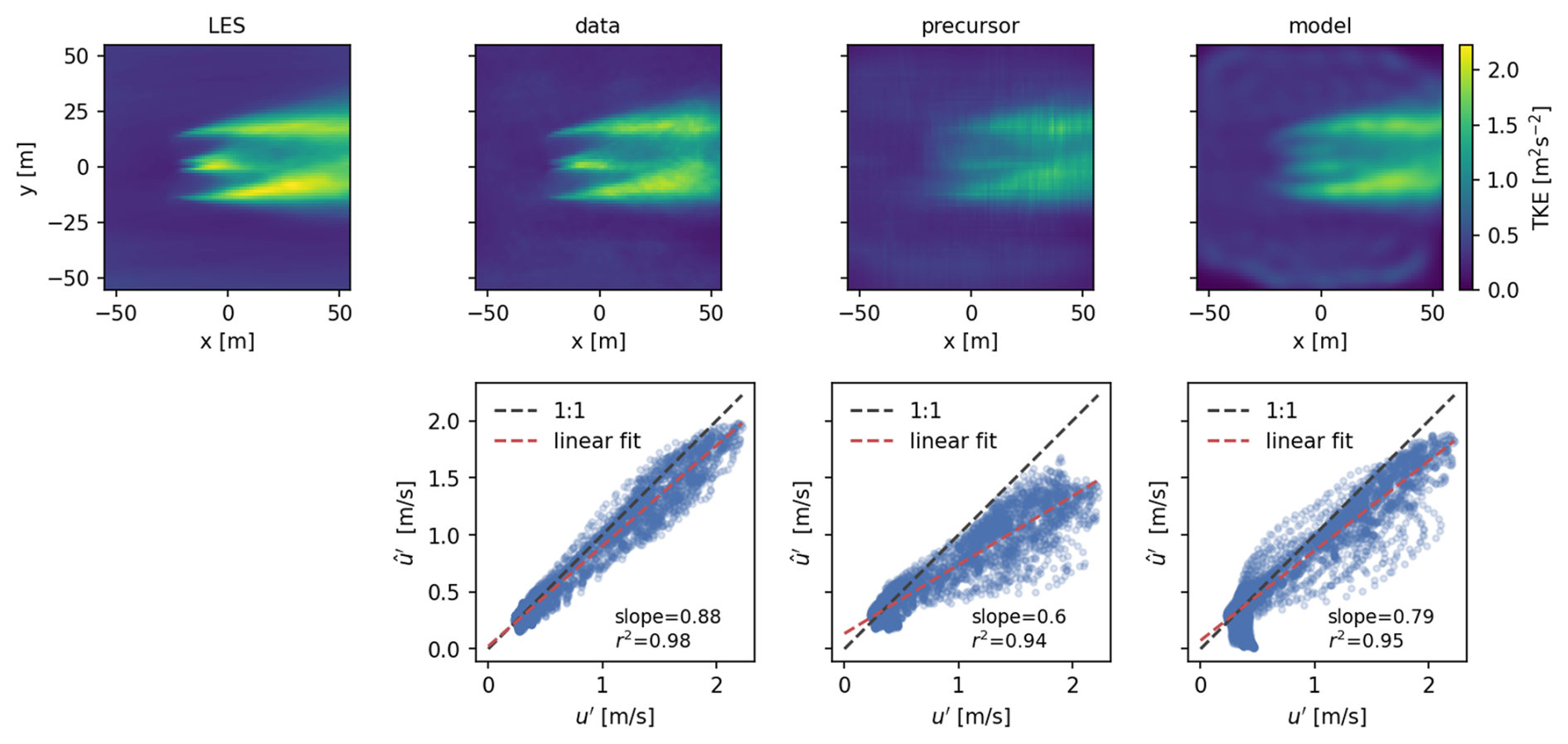
Figure 16 Comparisons of the TKE from the convective LES (top right) to the AT retrievals using the heterogeneous numerical covariance, the homogeneous numerical covariance from the precursor, and the analytical model (top row, from left). The bottom row compares respective TKE estimates to those from the LES, along with linear fit slope and coefficient of restitution.

To quantify the accuracy of the AT retrievals, Fig. 16 compares the horizontal turbulent kinetic energy (TKE = $(\stackrel{\mathrm{‾}}{u^{\prime \mathrm{2}}}+\stackrel{\mathrm{‾}}{v^{\prime \mathrm{2}}})/\mathrm{2})$ from the convective LES (top left) to the AT retrievals using the heterogeneous numerical covariance, the homogeneous numerical covariance from the precursor, and the analytical model. As for the variances in Fig. 15, the TKE estimated with AT is generally lower than the equivalent field from the LES. This relationship is highlighted in the linear regressions in the bottom row of Fig. 16, where the slope of the regression line is less than 1 for all retrieval methods. While the slope for the heterogeneous covariance retrievals is closest to 1, the slope for the homogeneous covariance from the precursor is significantly lower, indicating that the AT retrievals are not able to capture the full range of TKE in the LES. When using the analytical model, the slope is 0.79, better than the precursor correlations but still short of the heterogeneous case. There is also a small tail near the bottom-left corner of the linear regression corresponding to the corners of the AT domain where the analytical model is unable to make accurate estimates of any of the fluctuating fields.

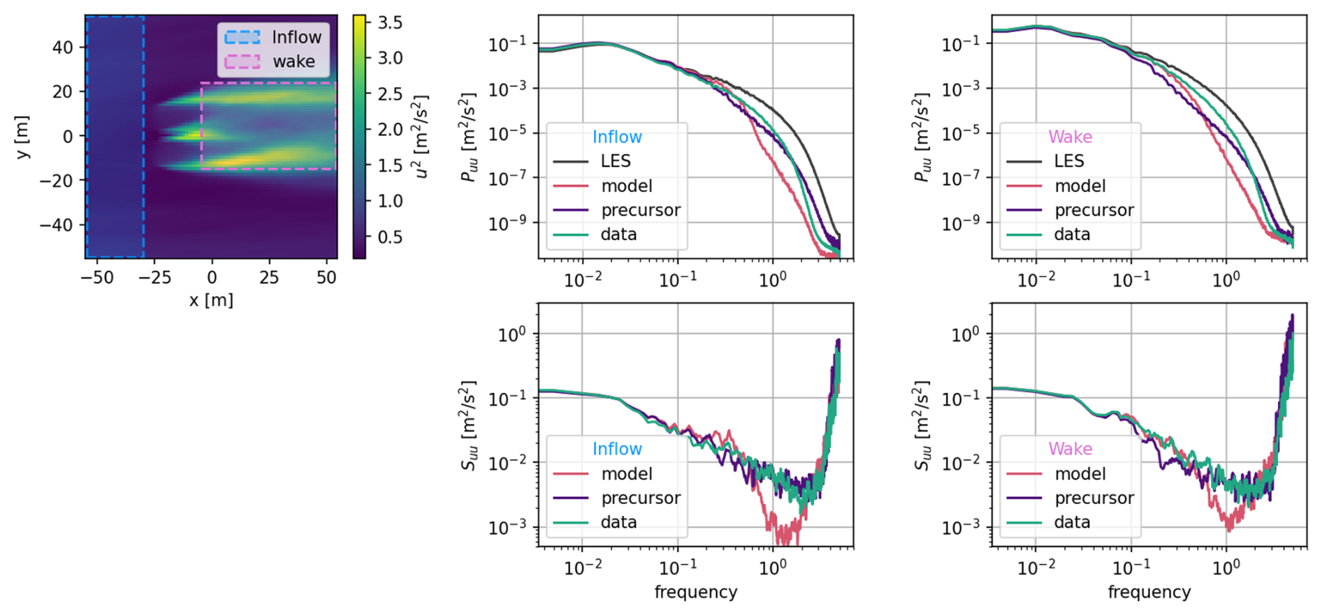
Figure 17 Spectra (top row) and coherence (bottom row) for the inflow (middle column) and wake (right column) subregions of the AT retrieval domain (left) for the convective case.

To evaluate AT’s ability to resolve wind turbine wake turbulence, Fig. 17 compares the spectra and coherence of streamwise velocity fluctuations in the inflow (left column) and wake (right column) regions of the AT retrieval domain. Spectra are calculated using Welch’s method, defined as

$$\begin{array}{}\text{(15)}& P_{u{}^{\prime }u{}^{\prime }}\left(f\right)={\displaystyle \frac{\mathrm{1}}{L}}\sum _{k=\mathrm{1}}^K{\displaystyle \frac{\mathrm{1}}{N}}{\left|\sum _{n=\mathrm{1}}^{N}u{{}^{\prime }}_k\left(n\right)e^{-i\mathrm{2}\mathit{\pi }fn/N}\right|}^{\mathrm{2}},\end{array}$$

where K is the number of segments, L=1024 samples is the number of points in the fast Fourier transform, N=2048 is the length of each segment, and $u{{}^{\prime }}_k\left(n\right)$ is the kth segment of the time series. A uniform window function is applied to each segment, zero-padded to mitigate convolution error introduced for finite time series.

Spectra are spatially averaged in the two subregions shown in Fig. 17, with the inflow region defined by $x/D<-\mathrm{0.5}$ and the wake region defined by $x/D>\mathrm{0.5}$ and $|y/D|<\mathrm{1}$. The inflow spectra exhibit lower power across all frequencies compared to the wake region, consistent with the lower TKE upstream of the turbine. The LES case shows a clear inertial subrange from approximately 0.01 to 1 Hz. All retrievals match the LES spectra well up to approximately 0.2 Hz. The heterogeneous covariance retrievals maintain agreement up to 2 Hz, outperforming the other methods. The analytical covariance model diverges from the LES most rapidly, showing significant deviation by 0.5 Hz. Above 2 Hz, the precursor-based retrieval shows slightly better agreement with the LES than the heterogeneous retrieval, suggesting that precursor correlations may better capture high-frequency inflow turbulence. In the wake region, similar trends are observed. The heterogeneous covariance model shows the best agreement up to 2 Hz. The precursor-based model again slightly outperforms the analytical model above 2 Hz, although both deviate from the LES more rapidly than the heterogeneous model.

Coherence between simulated and estimated streamwise velocity fluctuations quantifies the frequency-resolved agreement between the two signals and is computed as

$$\begin{array}{}\text{(16)}& S_{u\widehat{u}}\left(f\right)={\displaystyle \frac{\left|P_{u{}^{\prime }\widehat{u}{}^{\prime }}\right(f){|}^{\mathrm{2}}}{P_{u{}^{\prime }u{}^{\prime }}\left(f\right)P_{\widehat{u}{}^{\prime }\widehat{u}{}^{\prime }}\left(f\right)}},\end{array}$$

where $P_{u\widehat{u}{}^{\prime }}$ is the cross-spectral density, and $P_{u{}^{\prime }u{}^{\prime }}$ and $P_{\widehat{u}{}^{\prime }\widehat{u}{}^{\prime }}$ are the power spectral densities of the simulated and estimated fields, respectively. Coherence spectra are shown in the bottom row of Fig. 17 for the inflow and wake regions. At the lowest frequencies, $S_{u{}^{\prime }\widehat{u}{}^{\prime }}\approx \mathrm{0.15}$, indicating that AT retrievals fail to capture some low-frequency fluctuations in both inflow and wake regions. This is consistent with the reduced TKE observed in the AT reconstructions (Fig. 16). Coherence spectra reveal clear differences in the dynamic reconstruction ability of the covariance models. The heterogeneous covariance model consistently shows the best coherence with the LES between 0.1 and 2 Hz. The analytical model performs the worst in both inflow and wake regions, underestimating coherence across the full frequency range.

5 Discussion and conclusions

This study evaluates the fidelity of different covariance models in reconstructing fluctuating velocity and temperature fields using TDSI in wind turbine wakes in simulated ABLs. For both convective and neutral cases, heterogeneous covariance estimates from the turbine simulations yield the most accurate retrievals overall, particularly for streamwise velocity fluctuations u^′ and TKE. Analytical covariance models offer a consistent, lower-complexity alternative, but their performance varies across flow regimes and field variables.

Each approach to representing covariance in the TDSI has its limitations. Retrievals based on heterogeneous or precursor covariances exhibit numerical artifacts that align with the acoustic travel paths, particularly in the temperature retrievals. These artifacts reflect strong local anisotropies in the structure of the correlation functions and sensitivity to atmospheric stability. This behavior underscores the importance of accurate and representative covariance estimates in the reconstruction process, especially for thermodynamic variables.

The analytic covariance models, based on a Gaussian distribution, are each associated with a single length scale and standard deviation per variable. A more expressive covariance model, e.g., with directionally resolved length scales (l_u,x vs. l_u,y) or even heterogeneous parameters (e.g., l_ϕ=f(r)), could better represent flow features for wind turbine wakes and other industrial flows. Such refinements are expected to improve retrieval accuracy, particularly in strongly sheared or anisotropic flow regimes. However, care must be taken to ensure that additional model complexity does not compromise the generality of the method across atmospheric conditions or introduce prohibitive computational costs.

The analytical covariance models pursued in the traditional TDSI also make simplifications that should be revisited. For example, in the work by Vecherin et al. (2006), the authors assume that temperature and velocity fluctuations are not correlated, i.e., $C_{uT}=C_{vT}=\mathrm{0}$. In stratified ABLs, this simplification is not expected to hold, especially in configurations that seek vertical velocity fluctuations. The implementation of TDSI undertaken here also assumes that the correlation tensor is inherently symmetric. However, the tangential forcing introduced to the flow by a turbine rotor or actuator disk leads to a field where C_uv≠C_vu. These considerations would be a straightforward adaptation of the conventional TDSI and are expected to lead to improved representation of the coherent turbulence in a wind turbine wake.

Practical implementation of AT for field measurements must consider both retrieval accuracy and computational efficiency. The matrix A used in the retrieval scales with the number of ensemble frames N_f and the size of the spatial domain. While larger N_f typically reduces NRMSE, constructing A becomes increasingly expensive at high N_f. Heterogeneous numerical covariances can strike a balance when available, offering improved accuracy over analytical models and often outperforming precursor-based covariances at moderate N_f. However, computing A via path integrals of heterogeneous correlation functions requires simulations or other a priori estimates of the covariance structure, which may not be feasible in all scenarios. The three covariance estimates evaluated here bracket the practical design space from low-cost to high-fidelity. The primary purpose of the data model is to identify which aspects of the correlation structure affect retrieval accuracy most, thereby guiding the development of practical parameterized models applicable without full LES for every operating condition.

The error metrics used in the current work (NRMSE for velocity, RMSE for temperature) provide measures of retrieval accuracy with respect to the LES reference fields. However, this study represents an idealized assessment of AT performance. Several simplifying assumptions warrant acknowledgment: travel times are computed analytically from the forward model (Eq. (1)) rather than extracted from simulated acoustic waveforms, effectively assuming perfect time-of-flight retrieval with no timing errors and straight ray paths. Acoustic refraction due to temperature and wind-speed gradients is neglected; for the path lengths and near-neutral temperature gradients considered here (≲100 m, weak vertical lapse), ray bending is expected to produce travel-time deviations well below 1 ms (Wilson et al., 2015), smaller than the dominant retrieval uncertainties. Instrumental noise, multipath propagation, atmospheric absorption, and signal interference are not modeled. The virtual array assumes omnidirectional transducers with perfect colocated transmitter-receiver pairs. These idealizations establish an upper bound on retrieval performance; real-world deployments will face additional sources of uncertainty including wind-induced phase distortions, temperature lapse effects, and measurement error. Additional validation against field AT datasets is necessary to quantify retrieval uncertainty under operational conditions.

For field deployment near utility-scale wind turbines, several practical challenges must be addressed beyond those considered in this study. Differentiating the AT acoustic signals from aeroacoustic emissions from the turbine itself in the form of rotor noise presents a significant challenge if they overlap in the frequency domain. Broadband aeroacoustic emissions from blade–vortex interactions and turbulent boundary layer noise may corrupt acoustic signals along travel paths. To mitigate these impacts, future systems should endeavor to design chirps in the range of 100–500 Hz, below the peak rotor noise spectrum. Other strategies include coded pulse sequences that enable robust time-of-flight estimation in noisy environments, temporal gating to avoid blade-passage events, and array geometry optimization to minimize rotor-intersecting paths.

The NLR Flatirons Campus AT array operates in proximity to operating turbines and has demonstrated that signal identification and isolation techniques can successfully distinguish acoustic travel times from rotor noise, though further development is needed for wake-resolving configurations. Scaling to utility-scale turbines will require alternative array configurations such as vertical planar arrays spanning two meteorological towers or hybrid ground–aerial systems using uncrewed aerial systems. These alternative deployment strategies are explored in greater detail in a technical report (Hamilton and Maric, 2022). The 100 m × 100 m retrieval domain used here corresponds to approximately 3.7D for the V27. Scaling to modern rotors (D>120 m) would require a proportionally larger domain and transducer count, and systematic analysis of this scaling is deferred to future work.

Blending analytical models with numerically estimated anisotropies or introducing adaptive covariance models conditioned on local flow statistics may extend performance across regimes. The central approach to TDSI, mapping observations onto a model space by way of a linear operator, is also amenable to alternative inversion strategies. Other methods to estimate A, such as projection of the observed time of flight onto basis functions from dynamic mode decomposition, or scientific machine learning approaches, could further enhance retrieval accuracy and efficiency. The literature has already shown the success of some alternative strategies, including an unscented Kalman filter (Kolouri et al., 2013) and a radial basis function approach (Rogers and Finn, 2021). These improvements will be especially relevant for field-scale deployments near utility-scale wind turbines, where many of the assumptions in AT theory begin to break down. In future systems, flow heterogeneity, stratification, and sensor layout may all vary significantly, necessitating robust and generalizable inversion strategies. The performance of the heterogeneous covariance model in this study, especially in reconstructing the wake structure and dynamics, indicates strong potential for field application when supplemented by high-resolution LES or observational surrogates.

Appendix A: Supporting data – neutral case

The following figures supplement the main results by presenting correlation structure, reconstructed field statistics, and spectral diagnostics for the neutral ABL case.

Figure A1 shows numerically derived two-point correlation functions for the neutral precursor simulation, which serves as the basis for the homogeneous covariance model. The domain used for retrievals is indicated by the dashed outlines. These fields reveal broad, nearly isotropic structures consistent with weaker thermal stratification and more uniform turbulence generation.

Figure A2 presents analytical correlation models tuned to match the precursor correlations in Fig. A1. While the Gaussian form captures the general structure, differences in anisotropy and spatial decay – especially for $\stackrel{\mathrm{‾}}{u{}^{\prime }v{}^{\prime }}$ and $\stackrel{\mathrm{‾}}{{T^{\prime }}^{\mathrm{2}}}$ – highlight the limits of the analytical model’s expressiveness.

Figure A3 illustrates examples of the full tensor correlation field reconstructed from the turbine simulation. These highlight directional differences and localized anisotropy introduced by the wake, particularly in the streamwise correlations.

Figure A4 compares the LES-derived variances of the streamwise and spanwise velocity components, their covariance, and the temperature variance to the corresponding AT retrievals. Compared to the convective case, the neutral results show higher bias in the temperature variance and more spatially uniform retrieval errors across all variables.

Figure A5 presents reconstructed TKE from all three covariance models. While the heterogeneous numerical covariance model again yields the most accurate reconstruction, the differences among the models are smaller than in the convective case. The linear regression slopes and coefficients of restitution further indicate a general underestimation of TKE by all retrievals in this lower-energy regime.

Finally, Fig. A6 shows inflow and wake region spectra (top row) and coherence (bottom row) of the streamwise velocity fluctuations. Retrievals in the neutral case show stronger low-frequency attenuation compared to the convective case, with coherence values remaining below 0.2, even at the lowest frequencies. Nevertheless, relative model performance trends are consistent: heterogeneous covariance models provide the best spectral match, while the analytical model shows significant roll-off above 0.5 Hz.

Collectively, these results demonstrate that while TDSI is capable of resolving the main features of the neutral wake dynamics, reconstruction quality is reduced compared to the convective case, particularly for temperature fluctuations and low-frequency turbulent motions.

A mesh resolution study was conducted to assess the neutral turbulent boundary layer with the stand-alone Vestas V27 turbine, represented as a Joukowski actuator disk model, for both horizontally periodic and precursor-generated simulations. In all cases, the turbine is positioned at $(x,y)=(\mathrm{1100},\mathrm{1600})$ m. The resolution increases through the addition of static mesh refinement blocks, with three mesh configurations containing two, three, and four refinement levels. Each refinement zone reduces the grid spacing Δ by half in all three directions.

For horizontally periodic runs, refinement blocks lie in the range $\mathrm{0}<n<n_{\max }$, where n_max corresponds to the maximum refinement for each grid, spanning the entire domain length in the axial and lateral directions. In the vertical direction, these blocks extend to a height of 216 m from the ground. With the turbine included, an additional refinement zone at the n_max level spans −3D to 10D in the streamwise direction, ±3D in the lateral direction, and up to 189 m in height. The resulting grid spacings at the finest level are 2.5, 1.25, and 0.625 m for the three mesh configurations, providing 10.8, 21.6, and 43.2 points across the turbine diameter, respectively. For precursor-generated simulations, initial runs without the turbine use n=1 refinement (Δ=5 m), while turbine simulations employ n_max refinement levels.

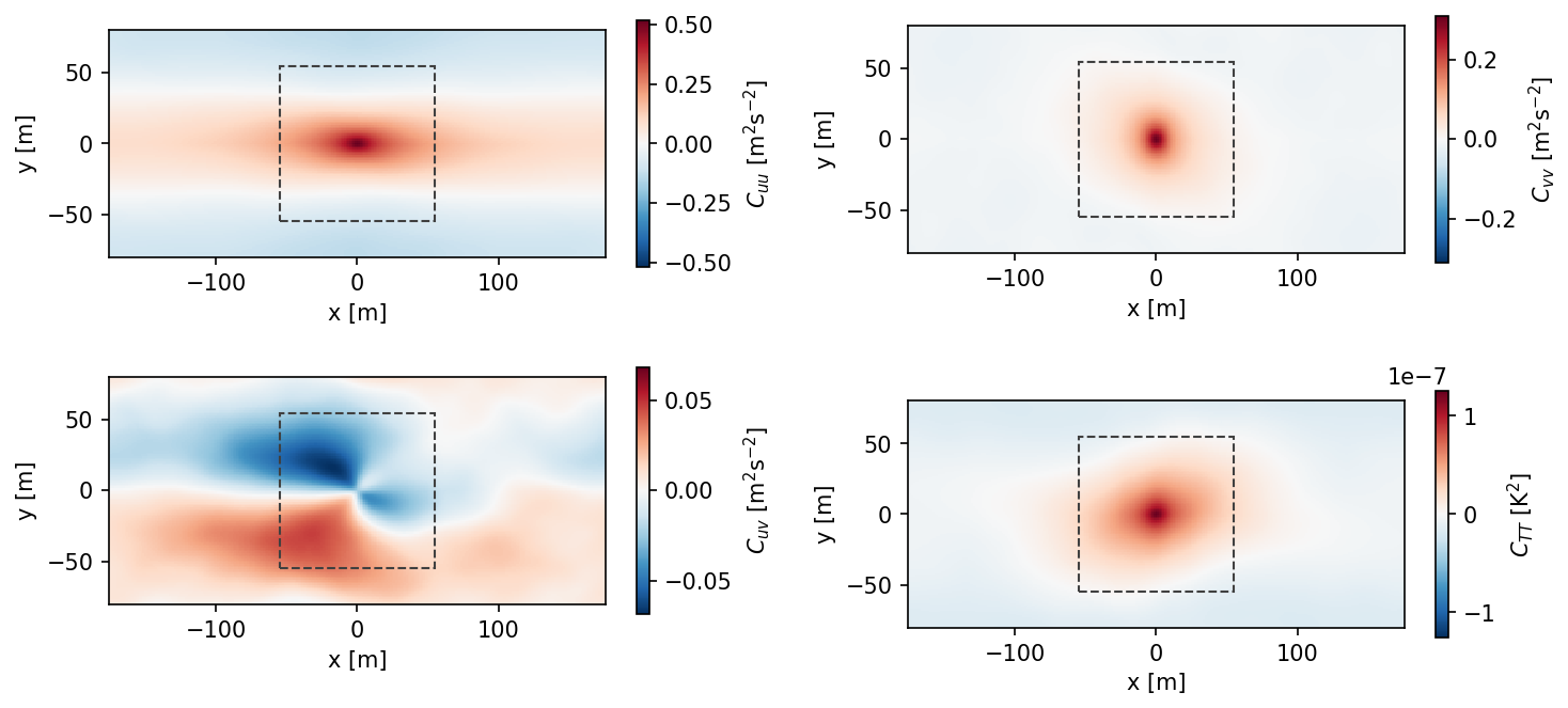
Figure A1 Numerically derived two-point correlation functions for the neutral precursor. Dashed region indicates the domain of the fluctuating field retrievals.

Figure A2 Modeled correlation functions from Eq. (8) for the neutral case tuned to match numerical correlation functions for the neutral precursor shown in Fig. A1. Model parameters correspond to those listed in Table 5.

.

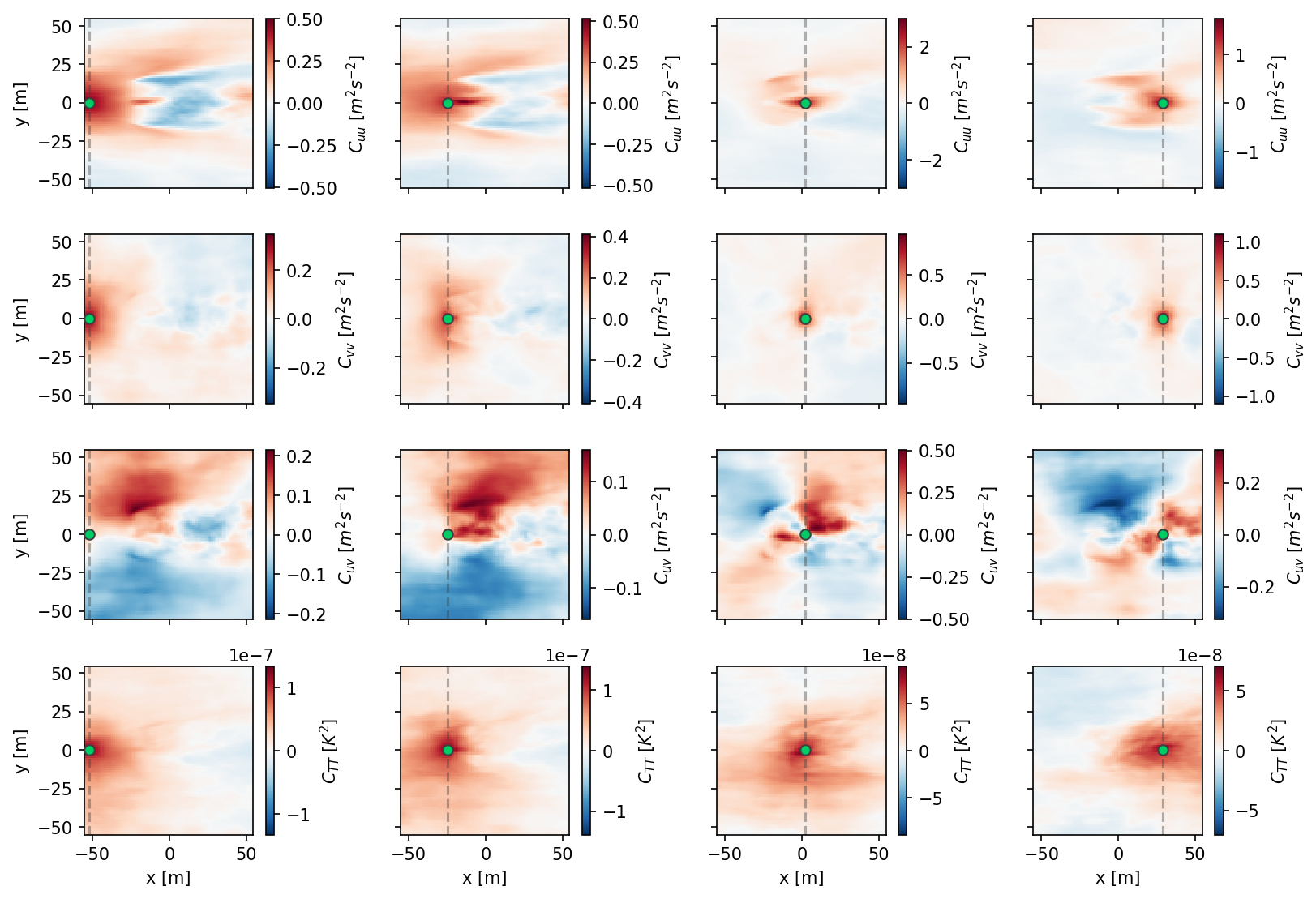
Figure A3 Examples of the correlation functions for the neutral wind turbine wake case. The central point (r) for each plot is indicated with a green marker. Vertical dashed gray lines indicate transects for which profiles are compared in Fig. 12.

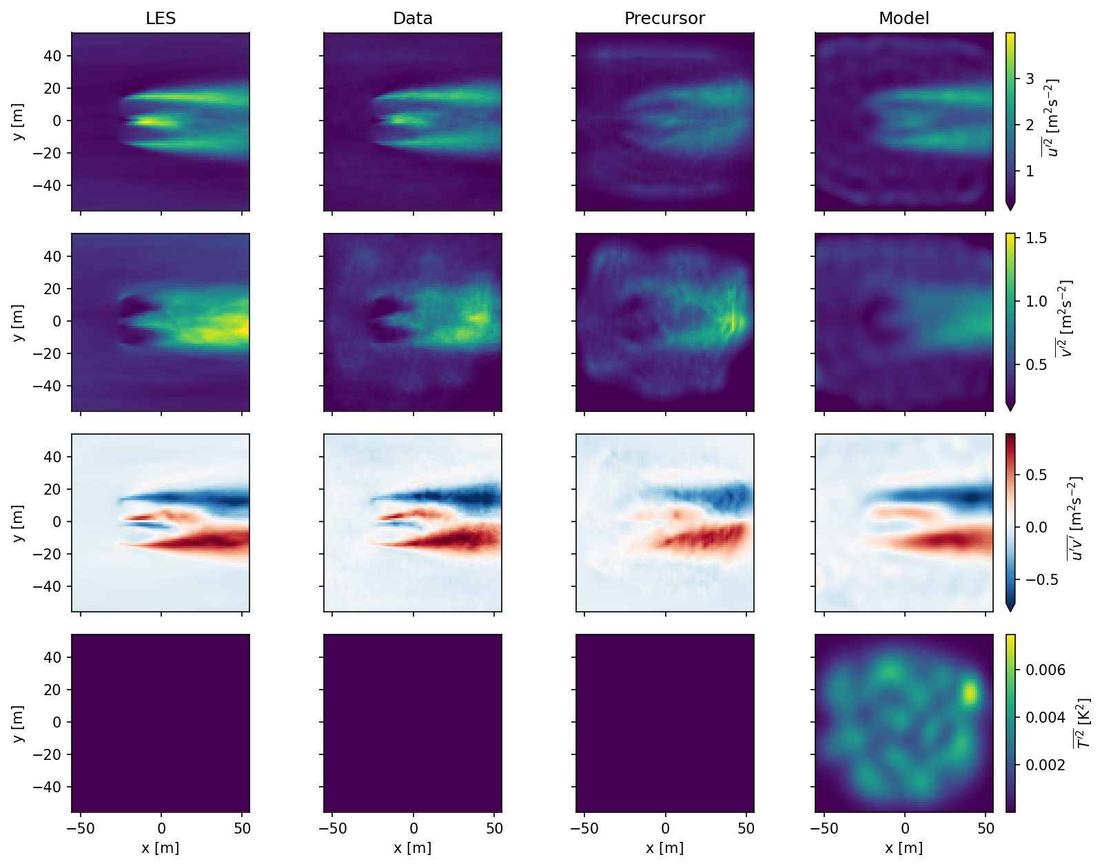
Figure A4 Comparison of the simulated variances of the streamwise and spanwise velocity components, their covariance, and the variance of temperature (from top) to the AT retrievals for the neutral case.

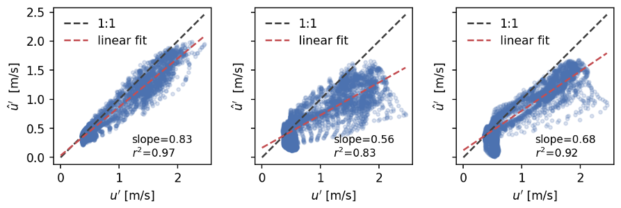
Figure A5 Comparisons of the TKE from the neutral LES (top right) to the AT retrievals using the heterogeneous numerical covariance, the homogeneous numerical covariance from the precursor, and the analytical model (from left). The bottom row compares respective TKE estimates to those from the LES, along with linear fit slope and coefficient of restitution.

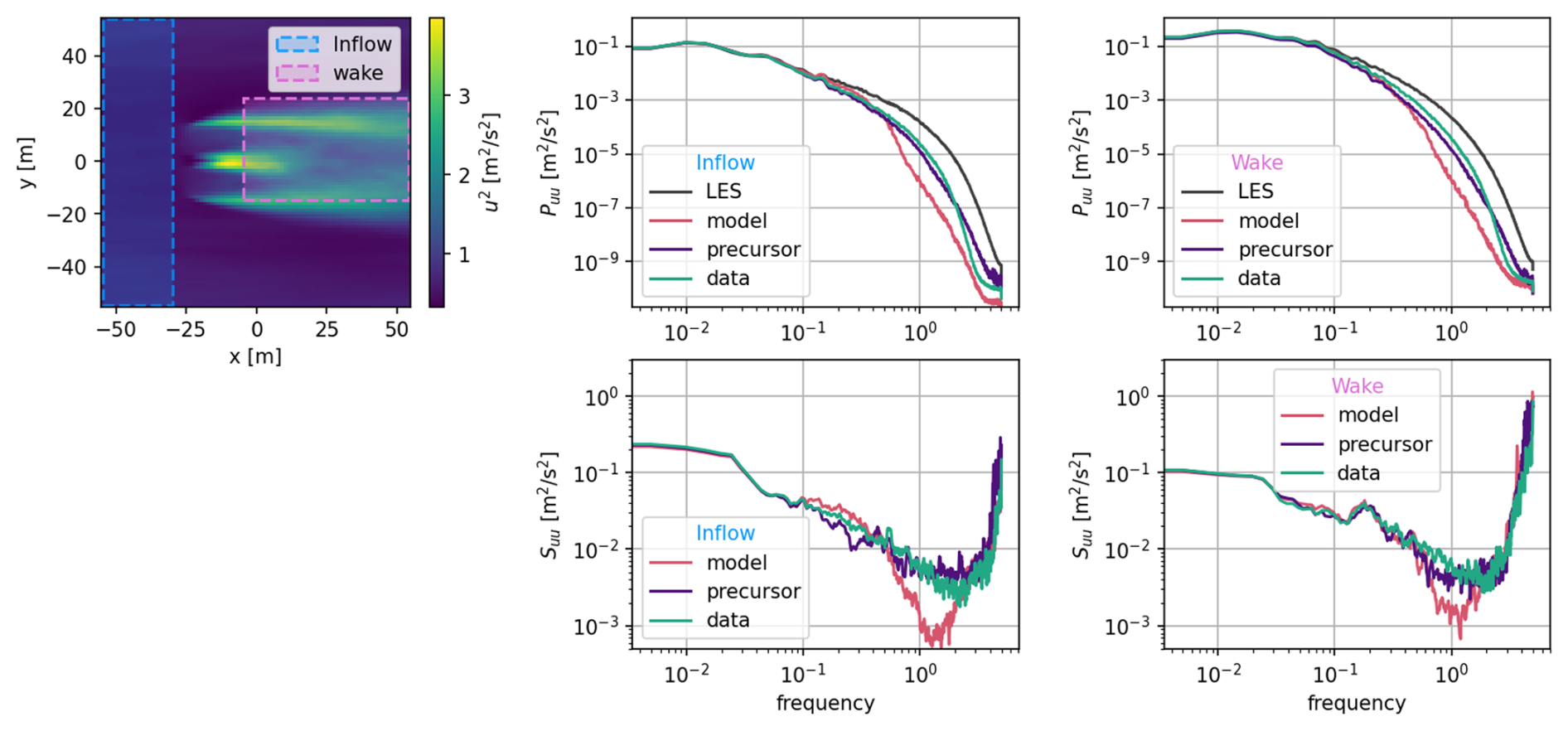
Figure A6 Spectra (top row) and coherence (bottom row) for the inflow (middle column) and wake (right column) subregions of the AT retrieval domain (left) for the neutral case.